Long memory and power law in coherency between realized

Long memory and power law in coherencybetween realized volatility and trading volume

Gilles de Truchis, Georgiana-Denisa Banulescu

Very preliminary draft

Abstract

The nature of the relationship between trading volume and volatility series has been widely studied

but overall, the literature provides mixed results. In this paper, we investigate this issue for the thirty

components of the Dow Jones stock market index in light of a recent concept named anti-cointegration.

For almost all firms, we show that the most persistent component of both trading volume and volatility

series is idiosyncratic and dwarfs a less persistent common factor that is undetectable by traditional long-

run or short-run econometric techniques. We also study the phase angle of the cross-spectrum and find

clear evidence that in presence of anti-cointegration, trading volume and volatility are contemporaneously

linked, thereby supporting the mixture of distributions hypothesis rather than the sequential arrival of

information hypothesis.

Keywords: anti-cointegration, realized volatility, trading volume, mixture distribution hypothesis,sequential arrival of informationJEL: C22, G10

1. Introduction

The nature of the relationship between trading volume and volatility in financial markets is an highly

debated issue. One strand of the literature argues in favor of a joint dependence of both variables upon

a common unobservable arrival of information process. This mixture of distributions hypothesis (MDH

hereafter), is theoretically discussed in Clark (1973), Tauchen and Pitts (1983), Andersen (1996) and

Liesenfeld (2001). Regarding empirical evidence in favor of the MDH, one can mention among others

Bollerslev and Jubinski (1999), Luu and Martens (2003), Ane and Ureche-Rangau (2008), Park (2010),

Jawadi and Ureche-Rangau (2013) and Rossi and Santucci de Magistris (2013a).1 Interestingly, most of

these studies account for the persistent nature of trading volume and volatility series, and thus investigate

∗This document is a work in progress.Email addresses: [email protected] (Gilles de Truchis), [email protected] (Georgiana-Denisa

Banulescu)1See also Harris (1986; 1987), Lamoureux and Lastrapes (1990) for earlier studies.

the possibility of a long-run dependence. As discussed in Bollerslev and Jubinski (1999), the rational for

this long-run version of the MDH is the possibility of heterogeneous responses to news in the short run.

The authors test this modified version of the MDH by simply investigating whether the long memory

behavior of both time series is similar. Rather than using GARCH-type models, they approximate the

volatility by the daily squared and absolute returns but unfortunately, those measures are very noisy.

More importantly, they do not formally test for the presence of a common long-run dependence (fractional

cointegration) although they mention this possibility as an interesting avenue for future research. Ane and

Ureche-Rangau (2008) go further in the long memory analysis and show that trading volume series are

uni-fractal processes whereas volatility series are multi-fractal processes. They argue that this divergent

scaling structure contradicts the MDH in the long run but that commonalities might exist in the short

run. Indeed, as argued earlier by Liesenfeld (2001), accounting for the long memory behavior of the

series is important but the possibility of short-run dependence should not be neglected. Using stochastic

volatility and GARCH-type models, the author finds that the volatility is more likely to be driven by the

information arrival process in the short run and by the sensitivity to the new information in the long

run. Conversely, the trading volume is essentially driven by the information arrival process whereas

the sensitivity to the new information is irrelevant. Luu and Martens (2003) consider both, a GARCH-

type model extended to de-trended volume and a bivariate VAR model with both volume and realized

volatility variables. The authors stress the importance of using the realized volatility and finally conclude

in favor of a bi-directional causality, thereby supporting the MDH. Park (2010) also uses a GARCH-

type approach but considers a modified version of the MDH, designed to incorporate both positive and

negative surprising information. The author finds results that are supportive of this modified MDH. Rossi

and Santucci de Magistris (2013a) pursue the analysis of Bollerslev and Jubinski (1999) and test for the

presence of fractional cointegration when the volatility is estimated by the realized variance. They find no

evidence of long run dependences. At the opposite, they find strong evidence of short-run non-Gaussian

extreme dependence by using a fractionally integrated VAR copula-based model.

A second strand of the literature argues that the information signal is disseminated randomly and

sequentially to market participants. Accordingly, the market equilibrium is only reached once all traders

have received the information and adjusted their positions. This sequential arrival of information (SAI)

theory has been developed by Copeland (1976), Jennings et al. (1981) and Smirlock and Starks (1988).

Because the SAI hypothesis implies the existence of incomplete equilibria during the dissemination pro-

cess, it also has strong implications with respect to the market efficiency. The SAI hypothesis has also find

many empirical supports in the literature (see e.g. Lobato and Velasco 2000, Nielsen 2009, Berger et al.

2009, Fleming and Kirby 2011, Mougoue and Aggarwal 2011, Tseng et al. 2015).2 Some of these studies

2See also Richardson and Smith (1994), Lamoureux and Lastrapes (1994), Hiemstra and Jones (1994) for earlier studies.

2

do not directly test for the SAI but the way they reject the MDH argues in favor of the SAI. For instance,

Fleming and Kirby (2011) investigate whether both series have a common long memory behavior but

using realized volatility measures. Conversely to Bollerslev and Jubinski (1999), they conclude against

this hypothesis and thus against the MDH. Berger et al. (2009) reformulate the volatility as a combina-

tion of the information flow and the market sensitivity to this information. Using fractional cointegration

techniques, they study the relationship between the trading volume and the market sensitivity and con-

clude against the MDH in the long run. In a very recent paper, Tseng et al. (2015) deal directly with the

SAI hypothesis on Exchange Traded Fund assets (ETF). They account for the persistent nature of the ETF

volatility by means of heterogeneous auto-regressive model and reveal that the trading volume contains

useful information to improve the prediction of the volatility. In an early study, Lobato and Velasco

(2000) address the MDH in a very interesting way, with a focus on the 30 components of the Dow Jones

index. In a first step they analyze the long memory behavior of each time series. In a second step, they

go further compared to Bollerslev and Jubinski (1999) and Fleming and Kirby (2011) by investigating

whether the squared coherency between both series is 1 at zero frequency, i.e. in “the very long run”.

Indeed, as demonstrated by Levy (2002) and Nielsen (2004), the (fractional) cointegration theory implies

a unit squared coherency at zero frequency. As they only find squared coherency below 0.4, they conclude

against the presence of fractional cointegration and thus against MDH. In this paper we go further in the

frequency domain analysis and our results leads to very different conclusions.

The MDH as well as the SAI hypothesis imply a positive relationship between trading volume and

volatility. Interestingly, some articles provide results that justify a negative relationship between the two

variables. For instance, Li and Wu (2006) adopt a microstructure approach and generalize the Andersen

(1996)’s model by decomposing trading volume into “informed” and “liquidity” components. They

identify that informed trading volume and volatility are positively correlated whereas liquidity volume

and volatility are negatively correlated and thus conclude in favor of the generalized MDH. Giot et al.

(2010) stress the importance of “good” and “bad” volatility, respectively related to the continuous and

the discontinuous jump components of the volatility. They find a positive relationship between trading

volume and “good” volatility and a negative relationship between trading volume and “bad” volatility

and hence, also conclude in favor of the MDH. Finally, Mougoue and Aggarwal (2011) essentially focus on

the possible nonlinear nature of the relationship between trading volume and volatility. They conclude in

favor of a bidirectional nonlinear Granger causality between both series but with a negative sign, thereby

concluding against the MDH.

In this paper we start from the long-run MDH of Bollerslev and Jubinski (1999) and consider the

thirty components of the Dow Jones stock market. In line with Lobato and Velasco (2000), we analyze

the squared coherency between trading volume and realized volatility series of each firms. Unlike them,

who only focus on the origin of the spectrum, we investigate the possibility of a power law coherency

3

at frequencies near but different from zero. This possibility is derived from the recent anti-cointegration

model of Sela and Hurvich (2012). For almost all firms, we find strong evidence that both, trading

volume and volatility are at least composed of two persistent components: a first component that is

very persistent and idiosyncratic and a second one that is less persistent and common to both series but

dwarfed by the first one. The presence of this persistent common factor is consistent with the aggregate

information-arrival process discussed in Bollerslev and Jubinski (1999). This new result might also

explain the mixed results of the literature and notably why neither fractional cointegration nor short run

techniques are able to detect clearly the common factor. As pointed out by Giot et al. (2010), the presence

of jumps might affect the relationship. Accordingly, we also use several jump-robust realized measures

as robustness check. Nonetheless, the results are unaffected, probably because jumps affect the spectrum

at higher frequencies. Regarding the mixture of distributions and the sequential arrival of information

hypotheses, we analyze the phase angle of the cross-spectrum and find in many cases clear evidence of

a contemporaneous dependence between both series. Accordingly, our study concludes in favor of the

MDH.3

The rest of the paper is organized as follows. In Section 2, we describe the data and the realized

measures that we consider. In Section 3, we conduct a rigorous analysis of the long memory behavior of

the series and we account for some specificities of the volatility. We also provide evidence of the fractional

cointegration failure. In Sections 4 and 5, we present the anti-cointegration model, the phase analysis and

we discuss the results. Section 6 concludes.

2. Data

As Lobato and Velasco (2000), we consider the 30 components of the Dow Jones index. Intraday data

are obtained from QuantQuote for the period January 3, 2000 to June 06, 2015 for a total of n = 4393 daily

observations. As argued in Gallant et al. (1993) and more recently in Mougoue and Aggarwal (2011),

there is strong evidence of nonlinear time trends in trading volume. Using a simple polynomial trend

regression we find strongly significant coefficients up to quadratic time trends for all series. Accordingly,

in the sequel of the paper, we work with the de-trended trading volume series.4

Concerning, the volatility, the literature generally consider either the model-free approach or the

GARCH-type approach. In the following, to avoid any misspecification risk, we adopt different realized

measures rather than GARCH-type models. We first consider the so-called realized variance estimator

3Focusing on the S&P500 and the NASDAQ 100, Kristoufek (2013) obtains similar result in time domain by means of power lawcross-correlation analysis.

4To remove the nonlinear deterministic trends, we prefer use the programmatic fitting algorithm of MATLAB based on theVandermonde matrix rather than the residuals of the polynomial regression. Indeed, the resulting series are more properly de-trended with the fitting method.

4

(RV hereafter) discussed in Andersen and Bollerslev (1997). The RV estimator is obtained by choosing a

sampling frequency ∆ (set to 5 minutes in our study) and by summing the M = 1/∆ squared intraday

returns over a day t so that

RVt(∆) =M

∑j=1

r2t,j

where rt,j = pt,j∆ − pt,(j−1)∆, with pt the logarithmic asset price. Assuming a continuous stochastic

volatility diffusion model for the price process and by the theory of quadratic variation, RVt(∆) converges

to the so-called integrated variance as M → ∞, i.e. RVt(∆)p−→∫ t

0 σ2s ds. Nonetheless, there is a large

consensus in the literature in favor of a jump-contaminated price dynamics implying that,

RVt(∆)p−→∫ t

t−1σ2(τ)dτ +

Nt

∑j=1

κ2t,j

where κj,t is the size of the jump j on day t and Nt is the number of jumps that day t. Regarding the

MDH, it is interesting to investigate whether the non-continuous part of the quadratic variation is likely

to impact the results. To disentangle the discrete and the continuous components, we first consider the

so-called bi-power variation (BPV) measure introduced by Barndorff-Nielsen and Shephard (2004):

BPVt(∆) =π

2M

M− 1

M−1

∑j=1|rt,j||rt,j+1|

As the frequency increases, the BPV converges to the integrated variance because a jump occurring at

time t will be multiplied by a very small return at time t + 1. In practice, the frequency is generally not

high enough to eliminate all jumps. Hence, we also consider the jump-robust measure introduced by

Andersen et al. (2012), named median realized variance (medRV hereafter) and defined as follows

medRVt(∆) =π

6− 4√

3 + π

(M

M− 2

) M−1

∑j=2

med(| rt,j−1 |, | rt,j |, | rt,j+1 |)2

Compared to the BPV estimator, the medRV is designed so that the impact of jumps completely vanishes

except in the case of two consecutive jumps (which is extremely rare at the sampling frequencies used in

empirical applications).

Another interesting issue that is likely to affect our results is the presence of microstructure frictions

like bid-ask bounce or infrequent trading when the sampling frequency is high. Barndorff-Nielsen et al.

(2008) deal with this issue by developing the so-called realized kernel (RK) estimator. The RK estimator

5

is given by

RKt(∆) =H

∑h=−H

k(h/(H + 1))γh,t

where H is a bandwidth determined by following the recommendations of Barndorff-Nielsen et al.

(2009), γh,t = ∑Mj=|h|+1 rt,jrt,j−|h| and k(.) is the Parzen kernel function. For robustness concerns, in the

sequel of the paper, we consider all these realized measures. However, to save place, we only report the

whole results when dissimilarities appear.

AC

F

Lags

Apple (median RV)

Asy

mpt

otic

AC

ovF

AC

F

Lags

Apple (Volume)

Asy

mpt

otic

AC

ovF

0 20 40 60 80 1000

0.2

0.4

0.6

0.8

1 = 0.396, m = 744

0.2

0.3

0.4

0.5

0.6

0.7δ

0 20 40 60 80 1000

0.5

1 = 0.397, m = 744

0

0.5

1δ

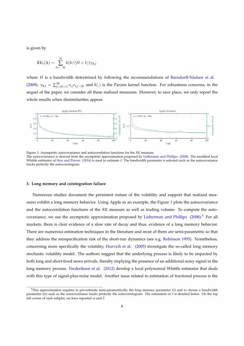
Figure 1: Asymptotic autocovariance and autocorrelation functions for the RK measure.The autocovariance is derived from the asymptotic approximation proposed by Lieberman and Phillips (2008). The modified localWhittle estimator of Hou and Perron (2014) is used to estimate δ. The bandwidth parameter is selected such as the autocovariancetracks perfectly the autocorrelogram

3. Long memory and cointegration failure

Numerous studies document the persistent nature of the volatility and support that realized mea-

sures exhibit a long memory behavior. Using Apple as an example, the Figure 1 plots the autocovariance

and the autocorrelation functions of the RK measure as well as trading volume. To compute the auto-

covariance, we use the asymptotic approximation proposed by Lieberman and Phillips (2008).5 For all

markets, there is clear evidence of a slow rate of decay and thus, evidence of a long memory behavior.

There are numerous estimation techniques in the literature and most of them are semi-parametric so that

they address the misspecification risk of the short-run dynamics (see e.g. Robinson 1995). Nonetheless,

concerning more specifically the volatility, Hurvich et al. (2005) investigate the so-called long memory

stochastic volatility model. The authors suggest that the underlying process is likely to be impacted by

both long and short-lived news arrivals, thereby implying the presence of an additional noisy signal in the

long memory process. Frederiksen et al. (2012) develop a local polynomial Whittle estimator that deals

with this type of signal-plus-noise model. Another issue related to estimation of fractional process is the

5This approximation requires to pre-estimate semi-parametrically the long memory parameter (δ) and to choose a bandwidthparameter (m) such as the autocovariance tracks perfectly the autocorrelogram. The estimation of δ is detailed below. On the topleft corner of each subplot, we have reported m and δ.

6

existence of spurious long memory, generally resulting from the presence of random level shifts or non-

linearities that contaminate the low frequencies. Hou and Perron (2014) suggest a modified local Whittle

(MLW) estimator to address the presence of both noise perturbations and low frequency contaminations.

Compared to the original local Whittle estimator of Robinson (1995), the MLW estimator, requires to

estimate two additional parameters and is defined as follows

(δ, θu, θw) = arg minδ,θu ,θw

Jm(δ, θu, θw)

Jm(δ, θu, θw) = log

(1m

m

∑j=1

I(λj)

g(λj)

)+

1m

m

∑j=1

log(g(λj)),

where g(λj) =(

λ−2δj + θw + (θu/n)λ−2

j

), δ is the long memory parameter, θu is the low frequency pa-

rameter, θw is the noise parameter, λj = (2π j)n−1 is the Fourier frequency, I(λj) is the periodogram and

m is the bandwidth parameter defined such as m = o(n).6 Conversely to traditional local Whittle-type

procedures, the bandwidth requirement is such that m > bn5/9c. In the following we only report the

results for m = bn0.8c but unreported results with different bandwidths are available upon request.

The Table 1 reports δ for all realized measures. The last column reports the asymptotic standard errors.

Overall, the coefficients are confined in the stationary regions and close to 0.4. Interestingly, δvo is close

to δrm for all stocks. The equality of integration orders of both series is a necessary but not sufficient

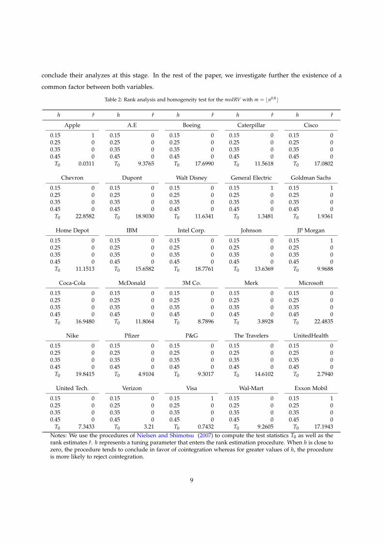
condition for the presence of cointegration. Hence, we rigorously test this hypothesis by applying the

procedure of Nielsen and Shimotsu (2007). Under the null hypothesis H0 : δvo = δrm this procedure

relies on a test statistic T0 that either converges in probability to 0 when both series are cointegrated or

converges to the χ21 distribution in absence of cointegration. Accordingly, we need to jointly analyze the

equality and the cointegration hypothesis. Fortunately, Nielsen and Shimotsu (2007) also suggest an

estimation procedure of the cointegration rank. This methodology relies on several tuning parameters

not detailed here. Nonetheless, notice that the results are generally sensible to the choice of a tuning

parameter defined as ν = m−h. When h is close to zero, the procedure tends to conclude in favor of

cointegration whereas for greater values of h, the procedure is more likely to reject cointegration. Thus,

we report the rank estimates for h = {0.15, 0.25, 0.35, 0.45}. Results of both, the equality test and the

rank estimation are reported in Table 2. Because we perform a pairwise analysis, the cointegration rank,

denoted r, is either 0 if there is no cointegration or 1 if there is cointegration.

In almost all cases, the cointegration rank estimates are equal to zero, thereby concluding against the

cointegration and thus against the presence of long run commonalities between volatility and trading vol-

6Notice that a confusion is possible between the financial and econometric terminologies because the word “frequency” appearsin both literature. However, in the present study, the word “frequency” always refers to frequency domain analysis and is related toeconometrics.

7

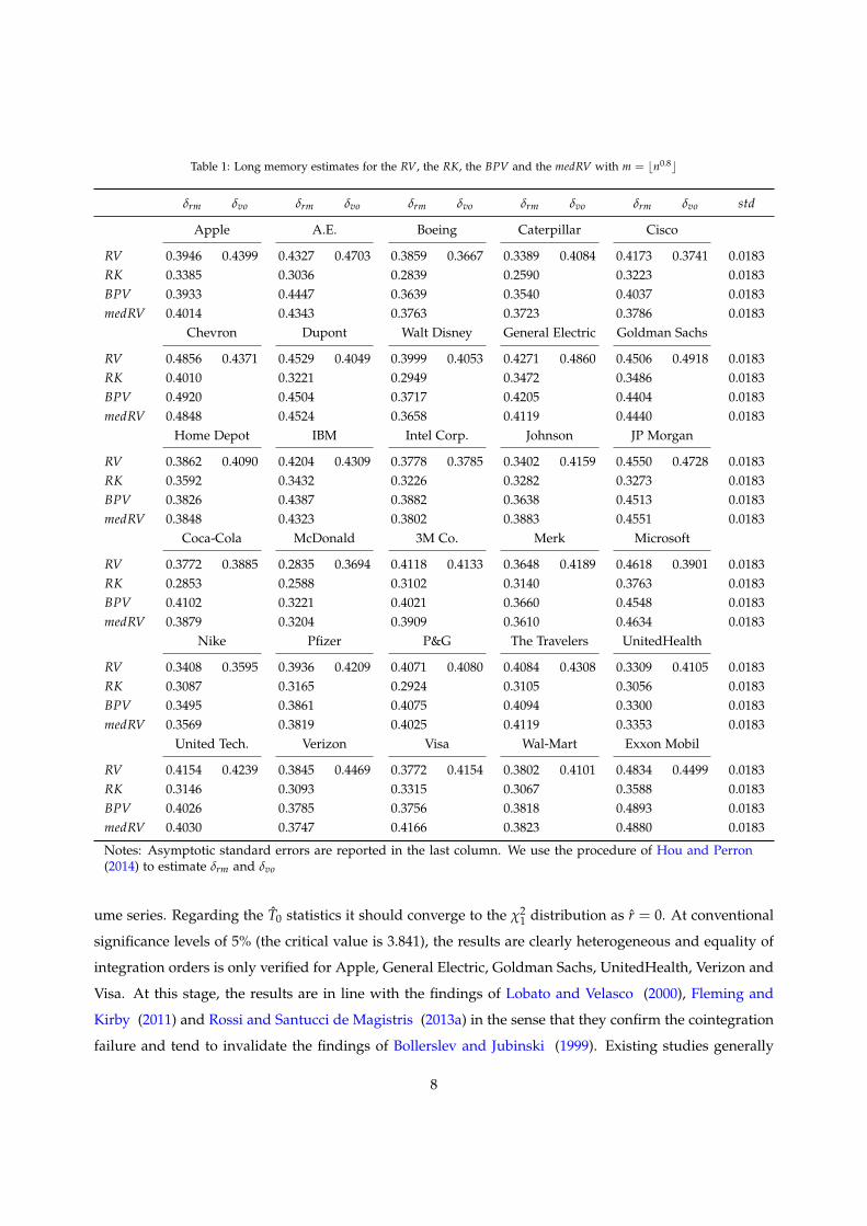
Table 1: Long memory estimates for the RV, the RK, the BPV and the medRV with m = bn0.8c

δrm δvo δrm δvo δrm δvo δrm δvo δrm δvo std

Apple A.E. Boeing Caterpillar Cisco

RV 0.3946 0.4399 0.4327 0.4703 0.3859 0.3667 0.3389 0.4084 0.4173 0.3741 0.0183RK 0.3385 0.3036 0.2839 0.2590 0.3223 0.0183BPV 0.3933 0.4447 0.3639 0.3540 0.4037 0.0183medRV 0.4014 0.4343 0.3763 0.3723 0.3786 0.0183

Chevron Dupont Walt Disney General Electric Goldman Sachs

RV 0.4856 0.4371 0.4529 0.4049 0.3999 0.4053 0.4271 0.4860 0.4506 0.4918 0.0183RK 0.4010 0.3221 0.2949 0.3472 0.3486 0.0183BPV 0.4920 0.4504 0.3717 0.4205 0.4404 0.0183medRV 0.4848 0.4524 0.3658 0.4119 0.4440 0.0183

Home Depot IBM Intel Corp. Johnson JP Morgan

RV 0.3862 0.4090 0.4204 0.4309 0.3778 0.3785 0.3402 0.4159 0.4550 0.4728 0.0183RK 0.3592 0.3432 0.3226 0.3282 0.3273 0.0183BPV 0.3826 0.4387 0.3882 0.3638 0.4513 0.0183medRV 0.3848 0.4323 0.3802 0.3883 0.4551 0.0183

Coca-Cola McDonald 3M Co. Merk Microsoft

RV 0.3772 0.3885 0.2835 0.3694 0.4118 0.4133 0.3648 0.4189 0.4618 0.3901 0.0183RK 0.2853 0.2588 0.3102 0.3140 0.3763 0.0183BPV 0.4102 0.3221 0.4021 0.3660 0.4548 0.0183medRV 0.3879 0.3204 0.3909 0.3610 0.4634 0.0183

Nike Pfizer P&G The Travelers UnitedHealth

RV 0.3408 0.3595 0.3936 0.4209 0.4071 0.4080 0.4084 0.4308 0.3309 0.4105 0.0183RK 0.3087 0.3165 0.2924 0.3105 0.3056 0.0183BPV 0.3495 0.3861 0.4075 0.4094 0.3300 0.0183medRV 0.3569 0.3819 0.4025 0.4119 0.3353 0.0183

United Tech. Verizon Visa Wal-Mart Exxon Mobil

RV 0.4154 0.4239 0.3845 0.4469 0.3772 0.4154 0.3802 0.4101 0.4834 0.4499 0.0183RK 0.3146 0.3093 0.3315 0.3067 0.3588 0.0183BPV 0.4026 0.3785 0.3756 0.3818 0.4893 0.0183medRV 0.4030 0.3747 0.4166 0.3823 0.4880 0.0183

Notes: Asymptotic standard errors are reported in the last column. We use the procedure of Hou and Perron(2014) to estimate δrm and δvo

ume series. Regarding the T0 statistics it should converge to the χ21 distribution as r = 0. At conventional

significance levels of 5% (the critical value is 3.841), the results are clearly heterogeneous and equality of

integration orders is only verified for Apple, General Electric, Goldman Sachs, UnitedHealth, Verizon and

Visa. At this stage, the results are in line with the findings of Lobato and Velasco (2000), Fleming and

Kirby (2011) and Rossi and Santucci de Magistris (2013a) in the sense that they confirm the cointegration

failure and tend to invalidate the findings of Bollerslev and Jubinski (1999). Existing studies generally

8

conclude their analyzes at this stage. In the rest of the paper, we investigate further the existence of a

common factor between both variables.

Table 2: Rank analysis and homogeneity test for the medRV with m = bn0.8c

h r h r h r h r h r

Apple A.E Boeing Caterpillar Cisco

0.15 1 0.15 0 0.15 0 0.15 0 0.15 00.25 0 0.25 0 0.25 0 0.25 0 0.25 00.35 0 0.35 0 0.35 0 0.35 0 0.35 00.45 0 0.45 0 0.45 0 0.45 0 0.45 0

T0 0.0311 T0 9.3765 T0 17.6990 T0 11.5618 T0 17.0802


0.15 0 0.15 0 0.15 0 0.15 1 0.15 10.25 0 0.25 0 0.25 0 0.25 0 0.25 00.35 0 0.35 0 0.35 0 0.35 0 0.35 00.45 0 0.45 0 0.45 0 0.45 0 0.45 0

T0 22.8582 T0 18.9030 T0 11.6341 T0 1.3481 T0 1.9361

Home Depot IBM Intel Corp. Johnson JP Morgan

0.15 0 0.15 0 0.15 0 0.15 0 0.15 10.25 0 0.25 0 0.25 0 0.25 0 0.25 00.35 0 0.35 0 0.35 0 0.35 0 0.35 00.45 0 0.45 0 0.45 0 0.45 0 0.45 0

T0 11.1513 T0 15.6582 T0 18.7761 T0 13.6369 T0 9.9688

Coca-Cola McDonald 3M Co. Merk Microsoft

0.15 0 0.15 0 0.15 0 0.15 0 0.15 00.25 0 0.25 0 0.25 0 0.25 0 0.25 00.35 0 0.35 0 0.35 0 0.35 0 0.35 00.45 0 0.45 0 0.45 0 0.45 0 0.45 0

T0 16.9480 T0 11.8064 T0 8.7896 T0 3.8928 T0 22.4835

Nike Pfizer P&G The Travelers UnitedHealth

0.15 0 0.15 0 0.15 0 0.15 0 0.15 00.25 0 0.25 0 0.25 0 0.25 0 0.25 00.35 0 0.35 0 0.35 0 0.35 0 0.35 00.45 0 0.45 0 0.45 0 0.45 0 0.45 0

T0 19.8415 T0 4.9104 T0 9.3017 T0 14.6102 T0 2.7940

United Tech. Verizon Visa Wal-Mart Exxon Mobil

0.15 0 0.15 0 0.15 1 0.15 0 0.15 10.25 0 0.25 0 0.25 0 0.25 0 0.25 00.35 0 0.35 0 0.35 0 0.35 0 0.35 00.45 0 0.45 0 0.45 0 0.45 0 0.45 0

T0 7.3433 T0 3.21 T0 0.7432 T0 9.2605 T0 17.1943Notes: We use the procedures of Nielsen and Shimotsu (2007) to compute the test statistics T0 as well as therank estimates r. h represents a tuning parameter that enters the rank estimation procedure. When h is close tozero, the procedure tends to conclude in favor of cointegration whereas for greater values of h, the procedureis more likely to reject cointegration.

9

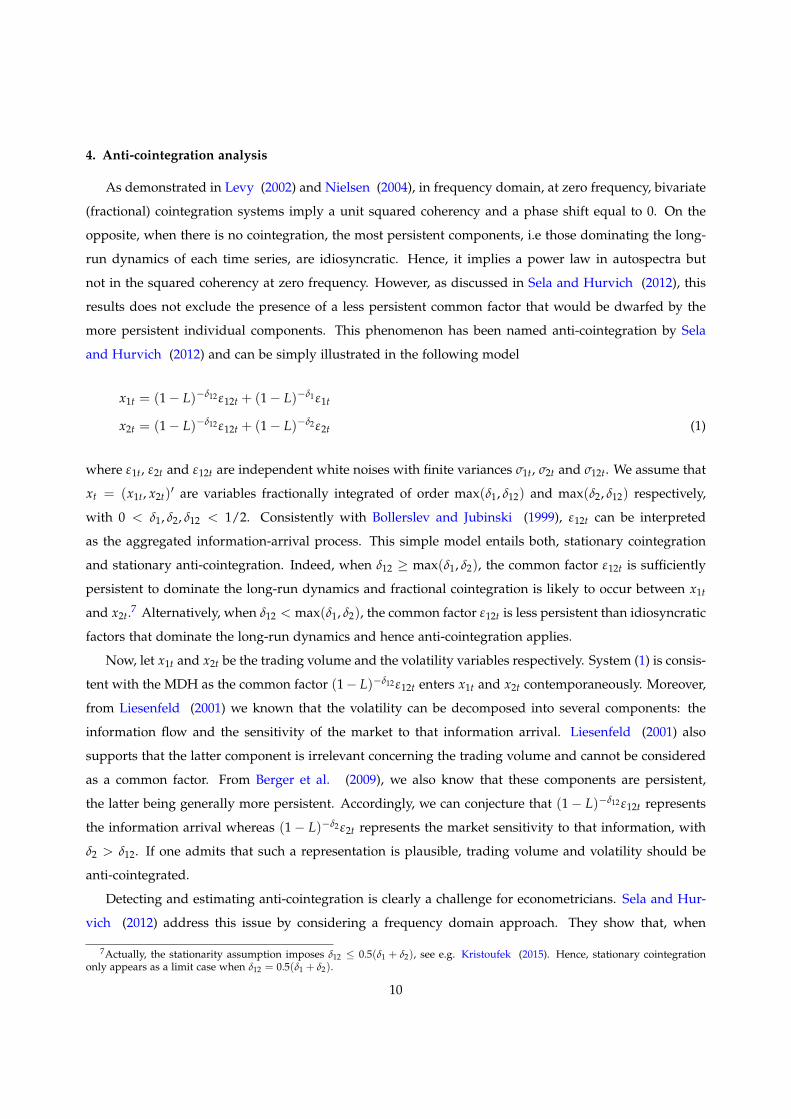
4. Anti-cointegration analysis

As demonstrated in Levy (2002) and Nielsen (2004), in frequency domain, at zero frequency, bivariate

(fractional) cointegration systems imply a unit squared coherency and a phase shift equal to 0. On the

opposite, when there is no cointegration, the most persistent components, i.e those dominating the long-

run dynamics of each time series, are idiosyncratic. Hence, it implies a power law in autospectra but

not in the squared coherency at zero frequency. However, as discussed in Sela and Hurvich (2012), this

results does not exclude the presence of a less persistent common factor that would be dwarfed by the

more persistent individual components. This phenomenon has been named anti-cointegration by Sela

and Hurvich (2012) and can be simply illustrated in the following model

x1t = (1− L)−δ12 ε12t + (1− L)−δ1 ε1t

x2t = (1− L)−δ12 ε12t + (1− L)−δ2 ε2t (1)

where ε1t, ε2t and ε12t are independent white noises with finite variances σ1t, σ2t and σ12t. We assume that

xt = (x1t, x2t)′ are variables fractionally integrated of order max(δ1, δ12) and max(δ2, δ12) respectively,

with 0 < δ1, δ2, δ12 < 1/2. Consistently with Bollerslev and Jubinski (1999), ε12t can be interpreted

as the aggregated information-arrival process. This simple model entails both, stationary cointegration

and stationary anti-cointegration. Indeed, when δ12 ≥ max(δ1, δ2), the common factor ε12t is sufficiently

persistent to dominate the long-run dynamics and fractional cointegration is likely to occur between x1t

and x2t.7 Alternatively, when δ12 < max(δ1, δ2), the common factor ε12t is less persistent than idiosyncratic

factors that dominate the long-run dynamics and hence anti-cointegration applies.

Now, let x1t and x2t be the trading volume and the volatility variables respectively. System (1) is consis-

tent with the MDH as the common factor (1− L)−δ12 ε12t enters x1t and x2t contemporaneously. Moreover,

from Liesenfeld (2001) we known that the volatility can be decomposed into several components: the

information flow and the sensitivity of the market to that information arrival. Liesenfeld (2001) also

supports that the latter component is irrelevant concerning the trading volume and cannot be considered

as a common factor. From Berger et al. (2009), we also know that these components are persistent,

the latter being generally more persistent. Accordingly, we can conjecture that (1− L)−δ12 ε12t represents

the information arrival whereas (1− L)−δ2 ε2t represents the market sensitivity to that information, with

δ2 > δ12. If one admits that such a representation is plausible, trading volume and volatility should be

anti-cointegrated.

Detecting and estimating anti-cointegration is clearly a challenge for econometricians. Sela and Hur-

vich (2012) address this issue by considering a frequency domain approach. They show that, when

7Actually, the stationarity assumption imposes δ12 ≤ 0.5(δ1 + δ2), see e.g. Kristoufek (2015). Hence, stationary cointegrationonly appears as a limit case when δ12 = 0.5(δ1 + δ2).

10

λ→ 0+, the coherency is of form

ρ(λ) ∼σ2

12σ1σ2

λ−2(δ12− 12 (δ1+δ2)), (2)

and has power law δρ = δ12 − 0.5(δ1 + δ2) when δρ < 0. Alternatively, when δ12 = 0.5(δ1 + δ2), there is no

power law coherency.

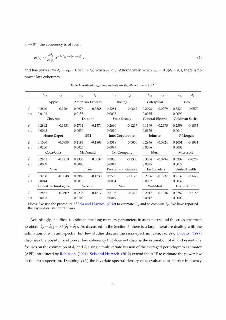
Table 3: Anti-cointegration analysis for the RV with m = bn0.8c

δ12 δρ δ12 δρ δ12 δρ δ12 δρ δ12 δρ

Apple American Express Boeing Caterpillar Cisco

δ 0.2840 -0.1264 0.0976 -0.3388 0.2284 -0.0862 0.2993 -0.0779 0.3320 -0.0570std 0.0102 0.0158 0.0033 0.0075 0.0090


δ 0.2842 -0.1531 0.2711 -0.1374 0.2690 -0.1217 0.1199 -0.2470 0.2358 -0.1853std 0.0048 0.0030 0.0010 0.0150 0.0040

Home Depot IBM Intel Corporation Johnson JP Morgan

δ 0.1580 -0.0958 0.2194 -0.1806 0.3318 0.0000 0.2936 -0.0924 0.2051 -0.1984std 0.0200 0.0025 0.0097 0.0056 0.0002

Coca-Cola McDonald 3M Company Merk Microsoft

δ 0.2661 -0.1210 0.2333 0.0037 0.3020 -0.1305 0.3034 -0.0794 0.3309 -0.0767std 0.0059 0.0003 0.0012 0.0025 0.0022

Nike Pfizer Procter and Gamble The Travelers UnitedHealth

δ 0.3208 -0.0048 0.2989 -0.1333 0.2596 -0.1173 0.2966 -0.1237 0.2132 -0.1477std 0.0044 0.0018 0.0054 0.0067 0.0032

United Technologies Verizon Visa Wal-Mart Exxon Mobil

δ 0.2882 -0.0509 0.2238 -0.1817 0.3197 -0.0413 0.2047 -0.1056 0.2787 -0.2183std 0.0003 0.0102 0.0019 0.0047 0.0002

Notes: We use the procedure of Sela and Hurvich (2012) to estimate δ12 and to compute δρ. We have reportedthe asymptotic standard errors.

Accordingly, it suffices to estimate the long memory parameters in autospectra and the cross-spectrum

to obtain δρ = δ12 − 0.5(δ1 + δ2). As discussed in the Section 3, there is a large literature dealing with the

estimation of δ in autospectra, but few studies discuss the cross-spectrum case, i.e. δ12. Lobato (1997)

discusses the possibility of power law coherency but does not discuss the estimation of δρ and essentially

focuses on the estimation of δ1 and δ2 using a multivariate version of the averaged periodogram estimator

(APE) introduced by Robinson (1994). Sela and Hurvich (2012) extend the APE to estimate the power law

in the cross-spectrum. Denoting f (λ) the bivariate spectral density of xt evaluated at Fourier frequency

11

λ, the cross-spectrum is simply given by

f12(λ) =√

f11(λ) f22(λ)ρ(λ)eiϕ12(λ),

where ϕ12(λ) is the phase difference defined in Equation (4) and ρ(λ) is the coherency approximated in

Equation (2) and defined at all frequencies by ρ(λ) = | f12(λ)|/( f11(λ) f22(λ))1/2 with | f12(λ)| the modulus

of f12(λ). In the vicinity of the origin, i.e. when λ→ 0, the spectral density can be approximated by

fkl(λ) ∼σkl2π

λ−δkl , {k, l} = {1, 2},

where δlk states for δ1 or δ2 when l = k = {1, 2} and δ12 when l , k = {1, 2}. In the univariate

case, Robinson (1994) suggests to use the averaged periodogram estimate (APE) of fll(λ) on m = o(n)

frequencies to define a semiparametric estimator of δll . Lobato (1997) extends the APE to the multivariate

case by considering the averaged periodogram matrix given by

F(λ) =2π

n

bnλ/2πc

∑j=1

I(λj), I(λ) =

(1√2πn

n

∑t=1

xteiλjt

)(1√2πn

n

∑t=1

xteiλjt

)∗.

However, the author assumes that δ12 = 0.5(δ1 + δ2). Sela and Hurvich (2012) relax this assumption and

thus obtain the following estimator of δkl ,

δkl =12−

log(|Fkl(qλm)|/|Fkl(λm)|

)2 log q

, q ∈ (0, 1), {k, l} = {1, 2}, (3)

For δll ∈ (0, 1/2) and l = 1, 2, this estimator is consistent with asymptotic normal distribution if δll < 1/4

and asymptotic non-normal distribution when δll > 1/4. When δ12 ∈ (0, 1/2), this estimator is also

consistent but Sela and Hurvich (2012) only investigate the limit theory for δ12 < 1/4. Accordingly, we

are not able to interpret the standard errors when δ12 > 1/4. In the following we set q = 0.5.

All results are reported in Tables 3, 4, 5 and 6 for m = bn0.8c. First of all, the cross-spectrum parameter

is less than δ1 and δ2 for almost all stocks and all realized measures. In some rare cases, Intel Corpora-

tion, McDonald and Nike present counterintuitive results with δρ > 0 but overall, the results are either

insignificant or negative. Unfortunately, in some cases, δ12 is greater than 1/4, so that we cannot use the

asymptotic standard errors computed and reported in parenthesis. In other cases, δ12 is generally signifi-

cant and δρ < 0 follows. Accordingly, we can conclude that in many cases, a power law coherency occurs,

revealing that the idiosyncratic persistent components of trading volume and volatility series dwarf a less

persistent common factor. This results is clearly original because neither the cointegration nor the tradi-

tional short-run techniques can detect this common factor. Moreover, as argued in Bollerslev and Jubinski

12

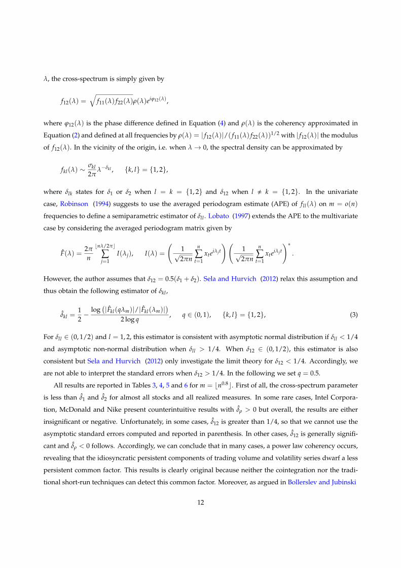
Table 4: Anti-cointegration analysis for the RK with m = bn0.8c



δ 0.2610 -0.1213 0.1023 -0.2696 0.2164 -0.0473 0.2862 -0.0511 0.3031 -0.0384std 0.0030 0.0197 0.0003 0.0031 0.0003


δ 0.2806 -0.1144 0.2487 -0.0944 0.2457 -0.0925 0.1217 -0.2052 0.2394 -0.1307std 0.0033 0.0046 0.0041 0.0190 0.0069


δ 0.1551 -0.0852 0.1997 -0.1617 0.2997 -0.0046 0.2892 -0.0908 0.1978 -0.1418std 0.0281 0.0048 0.0015 0.0031 0.0028


δ 0.2550 -0.0861 0.2292 0.0120 0.2791 -0.1026 0.2890 -0.0683 0.3136 -0.0513std 0.0013 0.0037 0.0063 0.0060 0.0043


δ 0.3133 0.0038 0.2865 -0.1071 0.2526 -0.0669 0.2819 -0.0894 0.2171 -0.1311std 0.0040 0.0059 0.0005 0.0195 0.0015


δ 0.2553 -0.0335 0.2091 -0.1589 0.3067 -0.0314 0.2001 -0.0735 0.2749 -0.1598std 0.0098 0.0017 0.0031 0.0007 0.0044


(1999), news are likely to persist over a random number of subsequent days so that the information-arrival

process is itself fractionally integrated. Accordingly, one can support that this common factor is related to

the information-arrival process. Interestingly, the results are robust to the choice of the realized measure,

thereby revealing that jumps do not affect the cross-spectrum around the frequencies at which occurs

the power-law coherency. This is not particularly surprising because one can expect that jumps affect the

spectrum at higher frequencies. In some sense, our findings are jump-robust because our semi-parametric

frequency domain approach is insensible to the presence of jumps. Our findings are also in line with Giot

et al. (2010) because they demonstrate that trading volume and volatility variables are only positively

related through the continuous component of the volatility.8

5. Phase spectrum analysis

At this stage, we cannot discriminate between the mixture of distribution and the sequential arrival

of information hypotheses. In this section we aim to address this question by analyzing the lead-lag

8Unreported robustness checks also reveal the insignificant impact of the bandwidth selection.

13

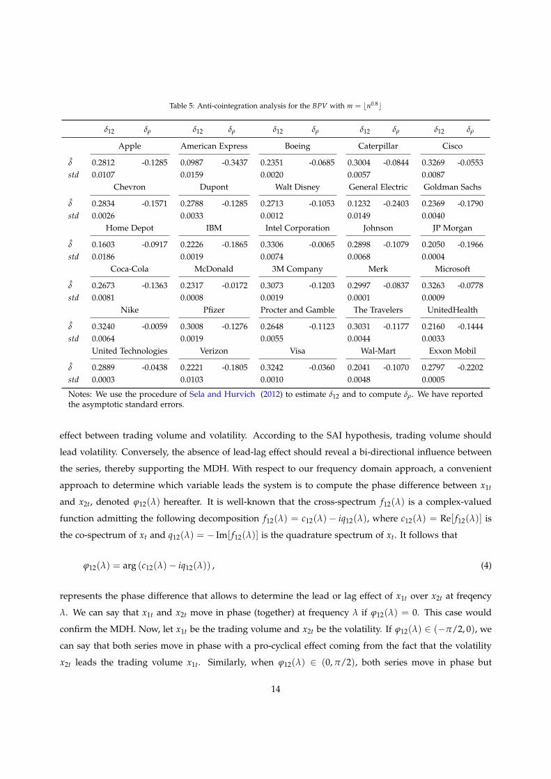
Table 5: Anti-cointegration analysis for the BPV with m = bn0.8c



δ 0.2812 -0.1285 0.0987 -0.3437 0.2351 -0.0685 0.3004 -0.0844 0.3269 -0.0553std 0.0107 0.0159 0.0020 0.0057 0.0087


δ 0.2834 -0.1571 0.2788 -0.1285 0.2713 -0.1053 0.1232 -0.2403 0.2369 -0.1790std 0.0026 0.0033 0.0012 0.0149 0.0040


δ 0.1603 -0.0917 0.2226 -0.1865 0.3306 -0.0065 0.2898 -0.1079 0.2050 -0.1966std 0.0186 0.0019 0.0074 0.0068 0.0004


δ 0.2673 -0.1363 0.2317 -0.0172 0.3073 -0.1203 0.2997 -0.0837 0.3263 -0.0778std 0.0081 0.0008 0.0019 0.0001 0.0009


δ 0.3240 -0.0059 0.3008 -0.1276 0.2648 -0.1123 0.3031 -0.1177 0.2160 -0.1444std 0.0064 0.0019 0.0055 0.0044 0.0033


δ 0.2889 -0.0438 0.2221 -0.1805 0.3242 -0.0360 0.2041 -0.1070 0.2797 -0.2202std 0.0003 0.0103 0.0010 0.0048 0.0005


effect between trading volume and volatility. According to the SAI hypothesis, trading volume should

lead volatility. Conversely, the absence of lead-lag effect should reveal a bi-directional influence between

the series, thereby supporting the MDH. With respect to our frequency domain approach, a convenient

approach to determine which variable leads the system is to compute the phase difference between x1t

and x2t, denoted ϕ12(λ) hereafter. It is well-known that the cross-spectrum f12(λ) is a complex-valued

function admitting the following decomposition f12(λ) = c12(λ)− iq12(λ), where c12(λ) = Re[ f12(λ)] is

the co-spectrum of xt and q12(λ) = − Im[ f12(λ)] is the quadrature spectrum of xt. It follows that

ϕ12(λ) = arg (c12(λ)− iq12(λ)) , (4)

represents the phase difference that allows to determine the lead or lag effect of x1t over x2t at freqency

λ. We can say that x1t and x2t move in phase (together) at frequency λ if ϕ12(λ) = 0. This case would

confirm the MDH. Now, let x1t be the trading volume and x2t be the volatility. If ϕ12(λ) ∈ (−π/2, 0), we

can say that both series move in phase with a pro-cyclical effect coming from the fact that the volatility

x2t leads the trading volume x1t. Similarly, when ϕ12(λ) ∈ (0, π/2), both series move in phase but

14

Table 6: Anti-cointegration analysis for the medRV with m = bn0.8c



δ 0.2817 -0.1321 0.0985 -0.3387 0.2356 -0.0742 0.3000 -0.0939 0.3266 -0.0430std 0.0116 0.0161 0.0021 0.0062 0.0085


δ 0.2849 -0.1520 0.2818 -0.1266 0.2762 -0.0974 0.1253 -0.2340 0.2376 -0.1802std 0.0029 0.0056 0.0008 0.0152 0.0038


δ 0.1585 -0.0946 0.2238 -0.1821 0.3308 -0.0023 0.2927 -0.1173 0.2056 -0.1979std 0.0205 0.0013 0.0079 0.0072 0.0008


δ 0.2695 -0.1230 0.2344 -0.0136 0.3067 -0.1154 0.3027 -0.0781 0.3287 -0.0797std 0.0067 0.0004 0.0055 0.0011 0.0026


δ 0.3227 -0.0108 0.3005 -0.1258 0.2677 -0.1069 0.3052 -0.1169 0.2180 -0.1450std 0.0079 0.0021 0.0033 0.0092 0.0036


δ 0.2881 -0.0449 0.2274 -0.1733 0.3229 -0.0578 0.2064 -0.1050 0.2827 -0.2166std 0.0001 0.0099 0.0002 0.0040 0.0003


with a pro-cyclical effect coming from the fact that the trading volume x1t leads the volatility x2t. This

case should confirm the SAI hypothesis. Conversely, if ϕ12(λ) ∈ (−π,−π/2) or ϕ12(λ) ∈ (π/2, π),

both series experiment an anti-phase movement (counter-cyclical) and either x1t leads x2t or x2t leads x1t

respectively. This result would be in line with Giot et al. (2010) and Mougoue and Aggarwal (2011)

because it would describe a negative relationship between the volume trading and the volatility. We can

also define, the time shift (i.e. the phase difference expressed in time units) of x1t over x2t at frequency λ

by τ12(λ) = ϕ12(λ)/λ. Notice that if we find no evidence of lead-lag effect, the model in Equations (1)

would be a plausible representation as it implies ϕ12(λ) = 0.

Results for all realized measures are reported in Tables 7 to 10.9 The first column of each table contains

the ordinary frequency (λ∗/2π) at which the power-law coherency occurs. More precisely, λ∗ represent

the frequency at which the squared coherency is maximal in the vicinity of the origin. To compute

the cross-spectrum, we use the Welch’s method associated to a modified Bartlett-Hann window. This

approach reduces the estimation bias but the sample size as well, so that the near-zero frequencies are

shifted to 0. Consequently, a power-law occurring very close to the origin might disappear. In such a

9Tables 8, 9 and 10 are in Appendix 7.2 as they present very similar figures.

15

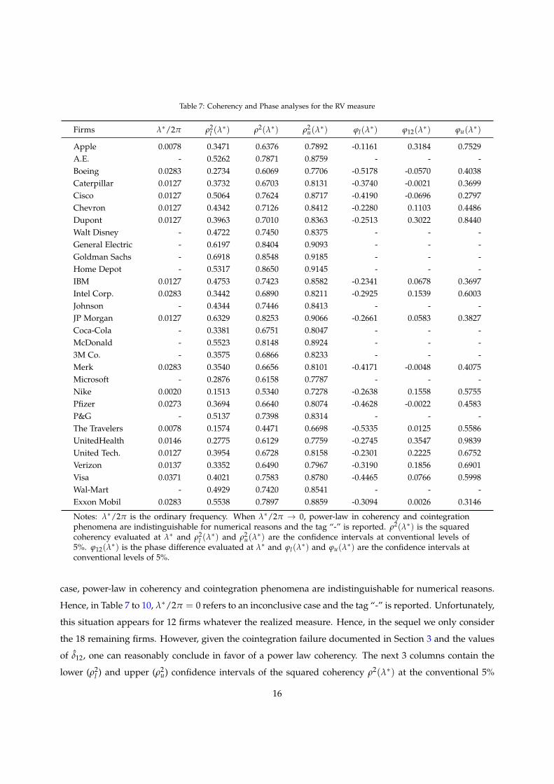
Table 7: Coherency and Phase analyses for the RV measure

Firms λ∗/2π ρ2l (λ∗) ρ2(λ∗) ρ2

u(λ∗) ϕl(λ

∗) ϕ12(λ∗) ϕu(λ∗)

Apple 0.0078 0.3471 0.6376 0.7892 -0.1161 0.3184 0.7529A.E. - 0.5262 0.7871 0.8759 - - -Boeing 0.0283 0.2734 0.6069 0.7706 -0.5178 -0.0570 0.4038Caterpillar 0.0127 0.3732 0.6703 0.8131 -0.3740 -0.0021 0.3699Cisco 0.0127 0.5064 0.7624 0.8717 -0.4190 -0.0696 0.2797Chevron 0.0127 0.4342 0.7126 0.8412 -0.2280 0.1103 0.4486Dupont 0.0127 0.3963 0.7010 0.8363 -0.2513 0.3022 0.8440Walt Disney - 0.4722 0.7450 0.8375 - - -General Electric - 0.6197 0.8404 0.9093 - - -Goldman Sachs - 0.6918 0.8548 0.9185 - - -Home Depot - 0.5317 0.8650 0.9145 - - -IBM 0.0127 0.4753 0.7423 0.8582 -0.2341 0.0678 0.3697Intel Corp. 0.0283 0.3442 0.6890 0.8211 -0.2925 0.1539 0.6003Johnson - 0.4344 0.7446 0.8413 - - -JP Morgan 0.0127 0.6329 0.8253 0.9066 -0.2661 0.0583 0.3827Coca-Cola - 0.3381 0.6751 0.8047 - - -McDonald - 0.5523 0.8148 0.8924 - - -3M Co. - 0.3575 0.6866 0.8233 - - -Merk 0.0283 0.3540 0.6656 0.8101 -0.4171 -0.0048 0.4075Microsoft - 0.2876 0.6158 0.7787 - - -Nike 0.0020 0.1513 0.5340 0.7278 -0.2638 0.1558 0.5755Pfizer 0.0273 0.3694 0.6640 0.8074 -0.4628 -0.0022 0.4583P&G - 0.5137 0.7398 0.8314 - - -The Travelers 0.0078 0.1574 0.4471 0.6698 -0.5335 0.0125 0.5586UnitedHealth 0.0146 0.2775 0.6129 0.7759 -0.2745 0.3547 0.9839United Tech. 0.0127 0.3954 0.6728 0.8158 -0.2301 0.2225 0.6752Verizon 0.0137 0.3352 0.6490 0.7967 -0.3190 0.1856 0.6901Visa 0.0371 0.4021 0.7583 0.8780 -0.4465 0.0766 0.5998Wal-Mart - 0.4929 0.7420 0.8541 - - -Exxon Mobil 0.0283 0.5538 0.7897 0.8859 -0.3094 0.0026 0.3146

Notes: λ∗/2π is the ordinary frequency. When λ∗/2π → 0, power-law in coherency and cointegrationphenomena are indistinguishable for numerical reasons and the tag “-” is reported. ρ2(λ∗) is the squaredcoherency evaluated at λ∗ and ρ2

l (λ∗) and ρ2

u(λ∗) are the confidence intervals at conventional levels of

5%. ϕ12(λ∗) is the phase difference evaluated at λ∗ and ϕl(λ

∗) and ϕu(λ∗) are the confidence intervals atconventional levels of 5%.

case, power-law in coherency and cointegration phenomena are indistinguishable for numerical reasons.

Hence, in Table 7 to 10, λ∗/2π = 0 refers to an inconclusive case and the tag “-” is reported. Unfortunately,

this situation appears for 12 firms whatever the realized measure. Hence, in the sequel we only consider

the 18 remaining firms. However, given the cointegration failure documented in Section 3 and the values

of δ12, one can reasonably conclude in favor of a power law coherency. The next 3 columns contain the

lower (ρ2l ) and upper (ρ2

u) confidence intervals of the squared coherency ρ2(λ∗) at the conventional 5%

16

significance level. ρ2(λ∗) represents the highest squared coherency away from the origin (when λ∗ > 0)

occurring at low frequencies. For all firms and all realized measures, ρ2(λ∗) is significantly different from

0 and generally greater than 0.6, revealing a strong degree of dependence between both variables. The

last 3 columns contain the lower (ϕl) and upper (ϕu) confidence intervals of the phase parameter ϕ12(λ∗)

at the conventional 5% significance level. It indicates whether or not trading volume and volatility series

move in phase at frequency λ∗ > 0. We are particularly interested by the phase parameter at this point

because the phase difference makes sense only when the squared coherency is significantly different from

zero and reasonably high.

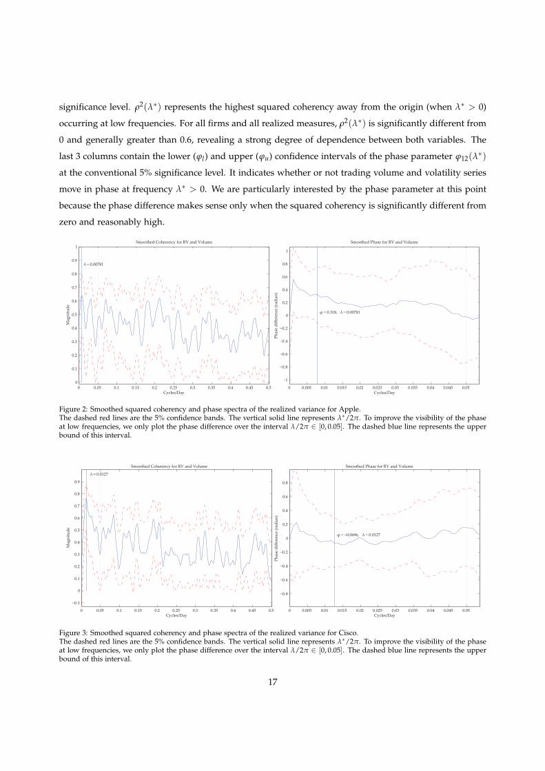
0 0.05 0.1 0.15 0.2 0.25 0.3 0.35 0.4 0.45 0.50

0.1

0.2

0.3

0.4

0.5

0.6

0.7

0.8

0.9

1

Cycles/Day

Mag

nitu

de

λ = 0.00781

Smoothed Coherency for RV and Volume

0 0.005 0.01 0.015 0.02 0.025 0.03 0.035 0.04 0.045 0.05

−1

−0.8

−0.6

−0.4

−0.2

0

0.2

0.4

0.6

0.8

1

Cycles/Day

Phas

e di

ffere

nce

(rad

ian)

φ = 0.318, λ = 0.00781

Smoothed Phase for RV and Volume

Figure 2: Smoothed squared coherency and phase spectra of the realized variance for Apple.The dashed red lines are the 5% confidence bands. The vertical solid line represents λ∗/2π. To improve the visibility of the phaseat low frequencies, we only plot the phase difference over the interval λ/2π ∈ [0, 0.05]. The dashed blue line represents the upperbound of this interval.

0 0.05 0.1 0.15 0.2 0.25 0.3 0.35 0.4 0.45 0.5

−0.1

0

0.1

0.2

0.3

0.4

0.5

0.6

0.7

0.8

0.9

Cycles/Day

Mag

nitu

de

= 0.0127

0 0.005 0.01 0.015 0.02 0.025 0.03 0.035 0.04 0.045 0.05

−0.8

−0.6

−0.4

−0.2

0

0.2

0.4

0.6

0.8

Cycles/Day

Phas

e di

ffere

nce

(rad

ian)

= −0.0696, = 0.0127

Smoothed Coherency for RV and Volume Smoothed Phase for RV and Volume

φ λ

λ

Figure 3: Smoothed squared coherency and phase spectra of the realized variance for Cisco.The dashed red lines are the 5% confidence bands. The vertical solid line represents λ∗/2π. To improve the visibility of the phaseat low frequencies, we only plot the phase difference over the interval λ/2π ∈ [0, 0.05]. The dashed blue line represents the upperbound of this interval.

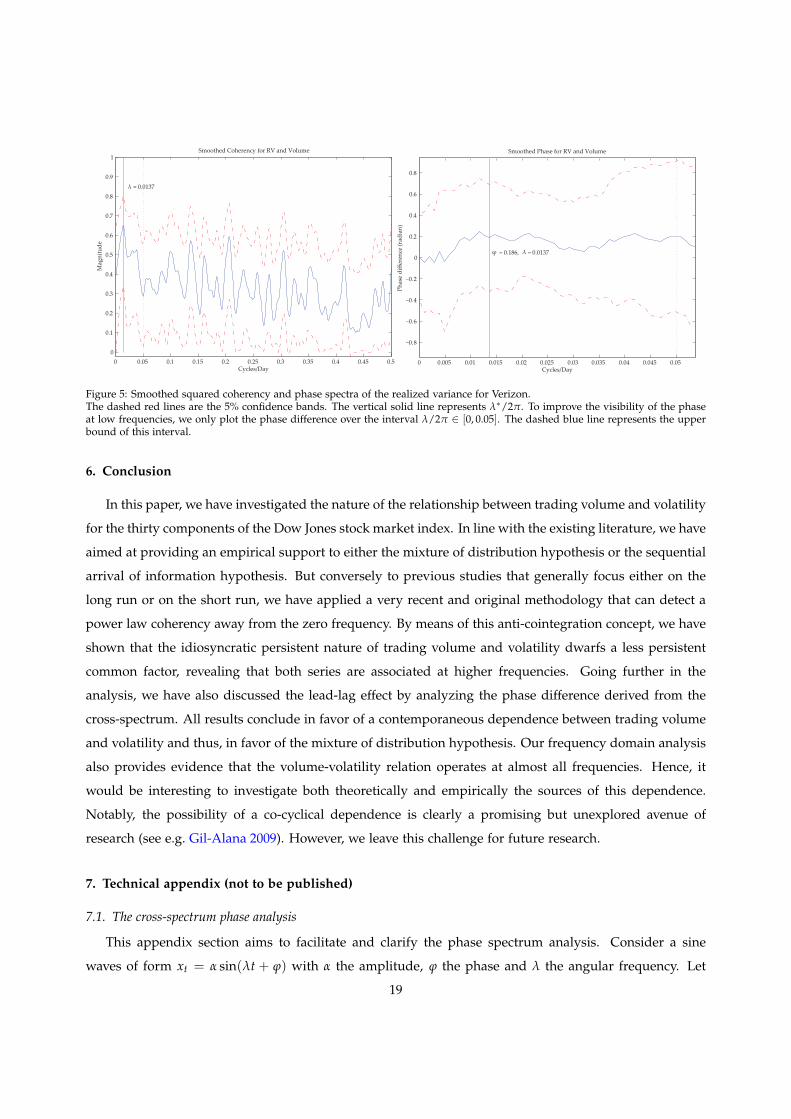
17

Overall, our findings provide strong evidence in favor of the MDH for 18 of the 30 firms composing

the Dow Jones index. Indeed, whatever the realized measure ϕ12 is not significantly different from zero

because zero is always in the confidence interval. In other words, both variables evolve contemporane-

ously with a positive correlation sign and we can reject the hypothesis of a pro-cyclical effect from one

variable to another as well as the hypothesis of an anti-phase co-movement, i.e. a negative correlation.

To give more intuition regarding the power law behavior documented in Section 4 and the phase

difference analysis, some illustrative cases are represented in Figures 2 to 5. The squared coherency is

reported on the left hand side whereas the phase difference is reported on the right hand side. The dashed

red lines represent the 5% confidence bands. The vertical solid line represents λ∗/2π. As λ∗/2π always

appears at lower frequencies than 0.05, we only plot the phase difference over the interval λ/2π ∈ [0, 0.05]

for a better visibility. The dashed blue line represents this arbitrary frontier of λ/2π = 0.05.

0 0.05 0.1 0.15 0.2 0.25 0.3 0.35 0.4 0.45 0.50

0.1

0.2

0.3

0.4

0.5

0.6

0.7

0.8

0.9

1

Cycles/Day

Mag

nitu

de

= 0.0283


0 0.005 0.01 0.015 0.02 0.025 0.03 0.035 0.04 0.045 0.05−1.2

−1

−0.8

−0.6

−0.4

−0.2

0

0.2

0.4

0.6

0.8

Cycles/Day

Phas

e di

ffere

nce

(rad

ian)

= 0.154,

= 0.0283


φ λ

λ

Figure 4: Smoothed squared coherency and phase spectra of the realized variance for Intel Corporation.The dashed red lines are the 5% confidence bands. The vertical solid line represents λ∗/2π. To improve the visibility of the phaseat low frequencies, we only plot the phase difference over the interval λ/2π ∈ [0, 0.05]. The dashed blue line represents the upperbound of this interval.

Interestingly, ρ2(λ) is generally significantly different from 0 at all frequencies although a slight down-

ward trend is evidenced. This general pattern might explain why the literature provides mixed results.

Indeed, the volume-volatility relationship seems to occur at many frequencies including the short and

the long run. However, it generally excludes the cointegration case. Moreover, the short run squared

coherency strongly depends on the firm considered. For instance, when λ → 0.5, the squared coherency

of Cisco is less than 0.1 whereas the one of Intel Corporation is greater than 0.6. Our analysis also cor-

roborates the findings of Lobato and Velasco (2000), i.e. ρ2(0) below 0.4. Indeed, Figures 2 to 5 reveal

that ρ2(0) is generally below 0.4, zero generally being included in the confidence interval. Finally, regard-

ing the phase difference curves, zero is always inside the confidence bands, revealing that the MDH is

strongly supported at low frequencies (λ < 0.05).

18

0 0.05 0.1 0.15 0.2 0.25 0.3 0.35 0.4 0.45 0.50

0.1

0.2

0.3

0.4

0.5

0.6

0.7

0.8

0.9

1

Cycles/Day

Mag

nitu

de

= 0.0137


0 0.005 0.01 0.015 0.02 0.025 0.03 0.035 0.04 0.045 0.05

−0.8

−0.6

−0.4

−0.2

0

0.2

0.4

0.6

0.8

Cycles/Day

Phas

e di

ffere

nce

(rad

ian)

= 0.186, = 0.0137


φ λ

λ

Figure 5: Smoothed squared coherency and phase spectra of the realized variance for Verizon.The dashed red lines are the 5% confidence bands. The vertical solid line represents λ∗/2π. To improve the visibility of the phaseat low frequencies, we only plot the phase difference over the interval λ/2π ∈ [0, 0.05]. The dashed blue line represents the upperbound of this interval.

6. Conclusion

In this paper, we have investigated the nature of the relationship between trading volume and volatility

for the thirty components of the Dow Jones stock market index. In line with the existing literature, we have

aimed at providing an empirical support to either the mixture of distribution hypothesis or the sequential

arrival of information hypothesis. But conversely to previous studies that generally focus either on the

long run or on the short run, we have applied a very recent and original methodology that can detect a

power law coherency away from the zero frequency. By means of this anti-cointegration concept, we have

shown that the idiosyncratic persistent nature of trading volume and volatility dwarfs a less persistent

common factor, revealing that both series are associated at higher frequencies. Going further in the

analysis, we have also discussed the lead-lag effect by analyzing the phase difference derived from the

cross-spectrum. All results conclude in favor of a contemporaneous dependence between trading volume

and volatility and thus, in favor of the mixture of distribution hypothesis. Our frequency domain analysis

also provides evidence that the volume-volatility relation operates at almost all frequencies. Hence, it

would be interesting to investigate both theoretically and empirically the sources of this dependence.

Notably, the possibility of a co-cyclical dependence is clearly a promising but unexplored avenue of

research (see e.g. Gil-Alana 2009). However, we leave this challenge for future research.

7. Technical appendix (not to be published)

7.1. The cross-spectrum phase analysis

This appendix section aims to facilitate and clarify the phase spectrum analysis. Consider a sine

waves of form xt = α sin(λt + ϕ) with α the amplitude, ϕ the phase and λ the angular frequency. Let

19

x1t, x2t, x3t and x4t be four sine waves, plotted in Figure 6 and defined as follows x1t = sin(λt + 0),

x2t = sin(λt + π/2) = cos(λt), x3t = sin(λt − π/2) and x4t = sin(λt − π). Figure 6 shows how the

phase moves the waves x2t, x3t and x4t away from x1t (that is the case where ϕ = 0). For x2t we have

ϕ2 = π/2: we observe that x2t moves to the left so that it leads x1t and the phase difference is negative

(ϕ12 = ϕ1 − ϕ2 < 0). For x3t we have ϕ3 = −π/2: we observe that x3t moves to the right so that it falls

behind and lags x1t. In this case, the phase difference is positive (ϕ12 = ϕ1 − ϕ2 > 0). For x4t we have

ϕ4 = −π: we observe that x4t moves so much to the right that it experiments an anti-phase movement

with x1t.

Figure 6: Impact of the phase parameter on sine waves

0 π/4 π/2 3π/4 π 5π/4 3π/2 7π/4 2π−1

−0.8

−0.6

−0.4

−0.2

0

0.2

0.4

0.6

0.8

1

Radian

Am

plitu

de

x1tx2tx3tx4t

(0 phase)

(leads )(lags )(anti-phase)

x1tx1t

The following example shows how to estimate the phase difference parameter ϕ12 = ϕ1 − ϕ2 when

signals are random. Consider x1t and x2t two random signals sampled at 1kHz and defined as x1t =

sin(2π400× t) + ε1t and x2t = 0.5 sin(2π400× t− π/2) + ε2t where ε1t and ε2t are Gaussian noises with

zero means, unit variances and uncorrelated at all frequencies. The two signals have a frequency of 400Hz

but compared to x1t, x2t has amplitude 0.5 and is phase-lagged by π/2. The two signals are plotted in

Figure 7.a and conversely to the previous case, the lead (or lag) effect is clearly visually undetectable.

Looking at the spectral squared coherence ρ(λ) plotted in Figure 7.b, we clearly observe a significant

increase in the coherency around 400Hz, consistently with the equation of x1t and x2t. Then, we compute

f12(λ), the cross-spectrum of both series and obtain the phase difference ϕ12 at each frequencies. The

parameter ϕ12 will only makes sense if the coherency is significantly different from 0, i.e. around the

frequency 400Hz. The Figure 7.c shows the phase spectrum and reveals that the phase difference at this

frequency is 0.487π. Compared to the true value that is ϕ12 = 0− ϕ2 = π/2, the bias is clearly weak.

20

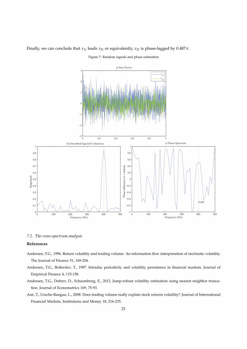
Finally, we can conclude that x1t leads x2t or equivalently, x2t is phase-lagged by 0.487π.

Figure 7: Random signals and phase estimation

0 0.2 0.4 0.6 0.8 1−3

−2

−1

0

1

2

3

x1tx2t

0 100 200 300 400 5000

0.1

0.2

0.3

0.4

0.5

0.6

0.7

0.8

0.9

1b) Smoothed Squared Coherence

Frequency (Hz)

c) Phase Spectrum

Phas

e di

ffere

nce

(π x

radi

an)

Mag

nitu

de

a) Sine Waves

0 100 200 300 400 500−1

−0.8

−0.6

−0.4

−0.2

0

0.2

0.4

0.6

0.8

1

Frequency (Hz)

0.487

7.2. The cross-spectrum analysis

References

Andersen, T.G., 1996. Return volatility and trading volume: An information flow interpretation of stochastic volatility.

The Journal of Finance 51, 169-204.

Andersen, T.G., Bollerslev, T., 1997. Intraday periodicity and volatility persistence in financial markets. Journal of

Empirical Finance 4, 115-158.

Andersen, T.G., Dobrev, D., Schaumburg, E., 2012. Jump-robust volatility estimation using nearest neighbor trunca-

tion. Journal of Econometrics 169, 75-93.

Ane, T., Ureche-Rangau, L., 2008. Does trading volume really explain stock returns volatility? Journal of International

Financial Markets, Institutions and Money 18, 216-235.

21

Table 8: Coherency and Phase analyses for the BPV measure


u(λ∗) ϕl(λ

∗) ϕ12(λ∗) ϕu(λ∗)

Apple 0.0283 0.3270 0.6441 0.7958 -0.2446 0.1397 0.5239A.E. - 0.5277 0.7886 0.8766 - - -Boeing 0.0283 0.2943 0.6130 0.7754 -0.4853 -0.0564 0.3725Caterpillar 0.0137 0.3820 0.6760 0.8161 -0.3731 0.0161 0.4053Cisco 0.0127 0.5106 0.7649 0.8731 -0.4455 -0.0908 0.2639Chevron 0.0127 0.4808 0.7404 0.8576 -0.2472 0.0856 0.4183Dupont 0.0127 0.3963 0.6952 0.8331 -0.2591 0.2952 0.8245Walt Disney - 0.4624 0.7753 0.8493 - - -General Electric - 0.6281 0.8474 0.9131 - - -Goldman Sachs - 0.6891 0.8534 0.9173 - - -Home Depot - 0.5345 0.9068 0.9398 - - -IBM 0.0127 0.4880 0.7485 0.8619 -0.2423 0.0656 0.3734Intel Corp. 0.0283 0.3333 0.6648 0.8064 -0.2982 0.1766 0.6496Johnson - 0.4396 0.7461 0.8499 - - -JP Morgan 0.0127 0.6418 0.8313 0.9098 -0.2754 0.0534 0.3823Coca-Cola - 0.3342 0.6729 0.8042 - - -McDonald - 0.5396 0.8020 0.8813 - - -3M Co. - 0.3744 0.6962 0.8297 - - -Merk 0.0283 0.3395 0.6575 0.8065 -0.3988 0.0550 0.5088Microsoft - 0.2984 0.6283 0.7867 - - -Nike 0.0029 0.1773 0.5445 0.7355 -0.2184 0.1520 0.5225Pfizer 0.0283 0.3725 0.6708 0.8088 -0.6098 -0.0950 0.4197P&G - 0.5144 0.7450 0.8362 - - -The Travelers 0.0078 0.1536 0.4604 0.6792 -0.5442 -0.0070 0.5302UnitedHealth 0.0137 0.2704 0.6065 0.7721 -0.3148 0.4266 1.1680United Tech. 0.0127 0.3675 0.6458 0.8000 -0.2425 0.2182 0.6789Verizon 0.0137 0.3127 0.6330 0.7884 -0.3380 0.1742 0.6864Visa 0.0371 0.3664 0.7435 0.8756 -0.4700 0.0720 0.6140Wal-Mart - 0.4973 0.7447 0.8555 - - -Exxon Mobil 0.0283 0.5186 0.7678 0.8729 -0.3335 -0.0170 0.2994


l (λ∗) and ρ2




Barndorff-Nielsen, O.E., Hansen, P.R., Lunde, A., Shephard, N., 2008. Designing Realized Kernels to Measure the ex

post Variation of Equity Prices in the Presence of Noise. Econometrica 76, 1481-1536.

Barndorff-Nielsen, O.E., Hansen, P.R., Lunde, A., Shephard, N., 2009. Realized kernels in practice: trades and quotes.

Econometrics Journal 12, 1-32.

Barndorff-Nielsen, O., Shephard, N., 2004. Power and bipower variation with stochastic volatility and jumps. Journal

of Financial Econometrics 2, 1-37.

22

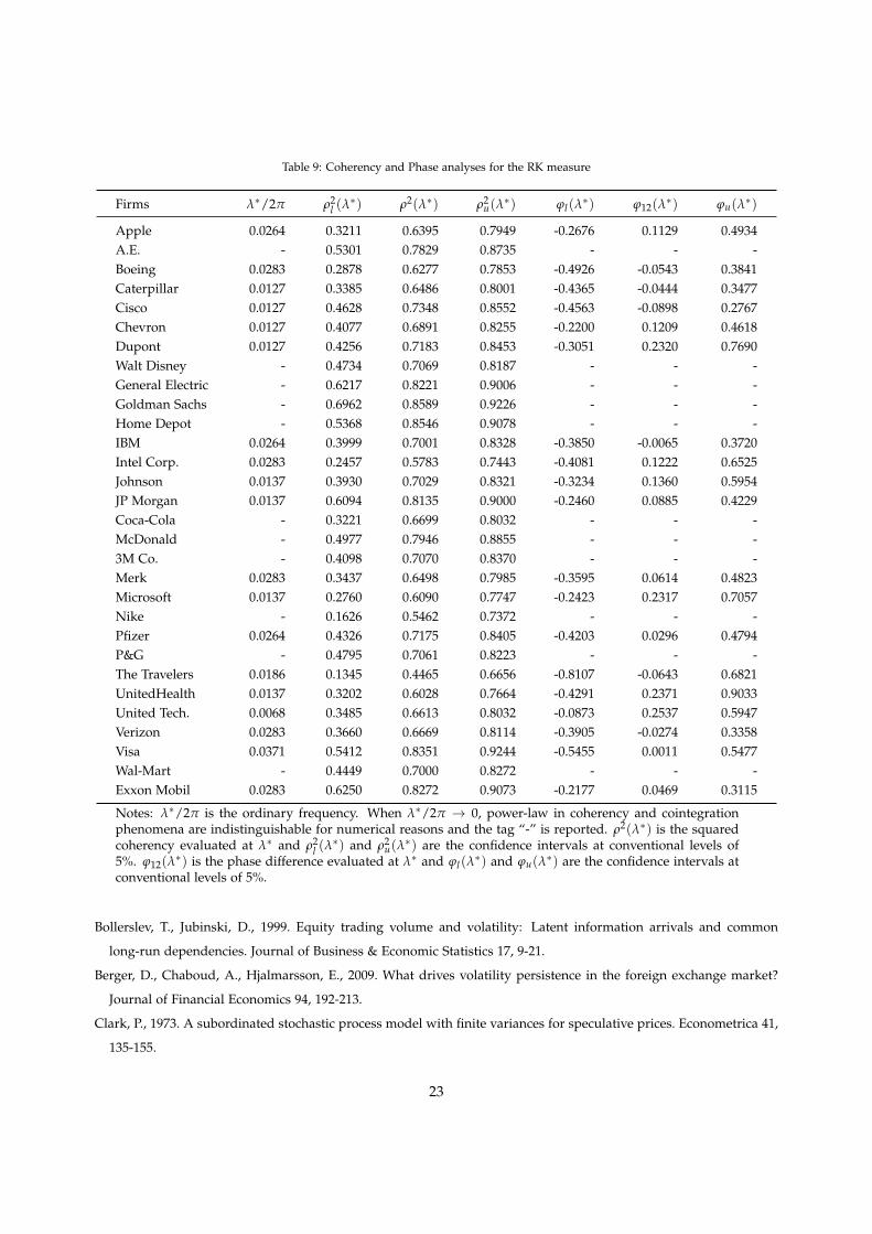
Table 9: Coherency and Phase analyses for the RK measure


u(λ∗) ϕl(λ

∗) ϕ12(λ∗) ϕu(λ∗)

Apple 0.0264 0.3211 0.6395 0.7949 -0.2676 0.1129 0.4934A.E. - 0.5301 0.7829 0.8735 - - -Boeing 0.0283 0.2878 0.6277 0.7853 -0.4926 -0.0543 0.3841Caterpillar 0.0127 0.3385 0.6486 0.8001 -0.4365 -0.0444 0.3477Cisco 0.0127 0.4628 0.7348 0.8552 -0.4563 -0.0898 0.2767Chevron 0.0127 0.4077 0.6891 0.8255 -0.2200 0.1209 0.4618Dupont 0.0127 0.4256 0.7183 0.8453 -0.3051 0.2320 0.7690Walt Disney - 0.4734 0.7069 0.8187 - - -General Electric - 0.6217 0.8221 0.9006 - - -Goldman Sachs - 0.6962 0.8589 0.9226 - - -Home Depot - 0.5368 0.8546 0.9078 - - -IBM 0.0264 0.3999 0.7001 0.8328 -0.3850 -0.0065 0.3720Intel Corp. 0.0283 0.2457 0.5783 0.7443 -0.4081 0.1222 0.6525Johnson 0.0137 0.3930 0.7029 0.8321 -0.3234 0.1360 0.5954JP Morgan 0.0137 0.6094 0.8135 0.9000 -0.2460 0.0885 0.4229Coca-Cola - 0.3221 0.6699 0.8032 - - -McDonald - 0.4977 0.7946 0.8855 - - -3M Co. - 0.4098 0.7070 0.8370 - - -Merk 0.0283 0.3437 0.6498 0.7985 -0.3595 0.0614 0.4823Microsoft 0.0137 0.2760 0.6090 0.7747 -0.2423 0.2317 0.7057Nike - 0.1626 0.5462 0.7372 - - -Pfizer 0.0264 0.4326 0.7175 0.8405 -0.4203 0.0296 0.4794P&G - 0.4795 0.7061 0.8223 - - -The Travelers 0.0186 0.1345 0.4465 0.6656 -0.8107 -0.0643 0.6821UnitedHealth 0.0137 0.3202 0.6028 0.7664 -0.4291 0.2371 0.9033United Tech. 0.0068 0.3485 0.6613 0.8032 -0.0873 0.2537 0.5947Verizon 0.0283 0.3660 0.6669 0.8114 -0.3905 -0.0274 0.3358Visa 0.0371 0.5412 0.8351 0.9244 -0.5455 0.0011 0.5477Wal-Mart - 0.4449 0.7000 0.8272 - - -Exxon Mobil 0.0283 0.6250 0.8272 0.9073 -0.2177 0.0469 0.3115


l (λ∗) and ρ2




Bollerslev, T., Jubinski, D., 1999. Equity trading volume and volatility: Latent information arrivals and common

long-run dependencies. Journal of Business & Economic Statistics 17, 9-21.

Berger, D., Chaboud, A., Hjalmarsson, E., 2009. What drives volatility persistence in the foreign exchange market?

Journal of Financial Economics 94, 192-213.

Clark, P., 1973. A subordinated stochastic process model with finite variances for speculative prices. Econometrica 41,

135-155.

23

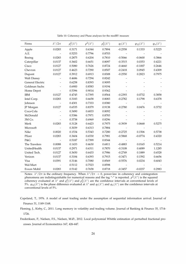
Table 10: Coherency and Phase analyses for the medRV measure


u(λ∗) ϕl(λ

∗) ϕ12(λ∗) ϕu(λ∗)

Apple 0.0283 0.3171 0.6344 0.7894 -0.2558 0.1333 0.5225A.E. - 0.5253 0.7796 0.8703 - - -Boeing 0.0283 0.2875 0.6204 0.7810 -0.5066 -0.0600 0.3866Caterpillar 0.0137 0.3602 0.6651 0.8097 -0.3515 0.0353 0.4221Cisco 0.0127 0.5080 0.7626 0.8724 -0.4660 -0.1007 0.2646Chevron 0.0127 0.4623 0.7290 0.8507 -0.2418 0.0945 0.4309Dupont 0.0127 0.3912 0.6913 0.8308 -0.2550 0.2823 0.7975Walt Disney - 0.4686 0.7294 0.8242 - - -General Electric - 0.6258 0.8393 0.9095 - - -Goldman Sachs - 0.6900 0.8583 0.9194 - - -Home Depot - 0.5396 0.9014 0.9362 - - -IBM 0.0127 0.4745 0.7395 0.8564 -0.2393 0.0732 0.3858Intel Corp. 0.0283 0.3183 0.6658 0.8083 -0.2782 0.1798 0.6378Johnson - 0.4301 0.7333 0.8380 - - -JP Morgan 0.0127 0.6535 0.8379 0.9138 -0.2780 0.0476 0.3732Coca-Cola - 0.3490 0.6833 0.8092 - - -McDonald - 0.5386 0.7971 0.8783 - - -3M Co. - 0.3738 0.6969 0.8296 - - -Merk 0.0283 0.3128 0.6423 0.7975 -0.3939 0.0668 0.5275Microsoft - 0.3039 0.6313 0.7884 - - -Nike 0.0020 0.1534 0.5343 0.7280 -0.2725 0.1506 0.5738Pfizer 0.0283 0.3604 0.6530 0.7981 -0.5868 -0.0774 0.4320P&G - 0.5187 0.7399 0.8344 - - -The Travelers 0.0088 0.1433 0.4630 0.6811 -0.4883 0.0165 0.5214UnitedHealth 0.0137 0.2971 0.6311 0.7870 -0.3108 0.4089 1.1285United Tech. 0.0127 0.3650 0.6433 0.7986 -0.2749 0.1889 0.6528Verizon 0.0137 0.3184 0.6393 0.7915 -0.3471 0.1592 0.6656Visa 0.0391 0.3146 0.7080 0.8569 -0.5576 0.0234 0.6043Wal-Mart - 0.5112 0.7523 0.8598 - - -Exxon Mobil 0.0283 0.5142 0.7658 0.8718 -0.3457 -0.0237 0.2983


l (λ∗) and ρ2




Copeland, T., 1976. A model of asset trading under the assumption of sequential information arrival. Journal of

Finance 31, 1149-1168.

Fleming, J., Kirby, C., 2011. Long memory in volatility and trading volume. Journal of Banking & Finance 35, 1714-

1726.

Frederiksen, P., Nielsen, F.S., Nielsen, M.Ø., 2012. Local polynomial Whittle estimation of perturbed fractional pro-

cesses. Journal of Econometrics 167, 426-447.

24

Gallant, R., Rossi, P., Tauchen, G., 1993. Nonlinear Dynamic Structures. Econometrica 61, 871-907.

Geweke, J., Porter-Hudak, S., 1983. The estimation and application of long memory time series models. Journal of

Time Series Analysis 4, 221-238.

Gil-Alana, L.A, 2009. A bivariate fractionally cointegrated relationship in the context of cyclical structures. Journal of

Statistical Computation and Simulation 79, 1355-1370.

Giot, P., Laurent, S., Petitjean, M., 2010. Trading activity, realized volatility and jumps. Journal of Empirical Finance

17, 168-175.

Harris, L., 1986. Cross-Security Tests of the Mixture of Distributions Hypothesis. Journal of Financial & Quantitative

Analysis 21, 39-46.

Harris, L., 1987. Transaction data test of the mixture of distributions hypothesis. Journal of Financial & Quantitative

Analysis 22(2), 127-141.

Hiemstra, C., Jones, J.D., 1994. Testing for Linear and Nonlinear Granger Causality in the Stock Price-Volume Relation.

Journal of Finance 49, 1639-1664.

Hou, J., Perron, P., 2014. Modified local Whittle estimator for long memory processes in the presence of low frequency

(and other) contaminations. Journal of Econometrics 182, 309-328.

Hurvich, C.M., Moulines, E., Soulier, P., 2005. Estimating long memory in volatility. Econometrica 73, 1283-1328.

Luu, J.C., Martens, M., 2003. Testing the mixture-of-distributions hypothesis using “realized” volatility. Journal of

Futures Markets 23, 661-679.

Jawadi, F., Ureche-Rangau, L., 2013. Threshold linkages between volatility and trading volume: Evidence from devel-

oped and emerging markets. Studies in Nonlinear Dynamics and Econometrics 17, 313-333.

Jennings, R.H., Starks, L.T., Fellingham, J.C., 1981. An Equilibrium Model of Asset Trading with Sequential Informa-

tion Arrival. Journal of Finance 36, 143-161.

Johansen, S., Nielsen, M.Ø., 2012. Likelihood Inference for a Fractionally Cointegrated Vector Autoregressive Model.

Econometrica 80, 2667-2732.

Kristoufek, L., 2013. Testing power-law cross-correlations: rescaled covariance test. The European Physical Journal B

86, 418.

Kristoufek, L. (2015). Can the bivariate Hurst exponent be higher than an average of the separate Hurst exponents?

Physica A: Statistical Mechanics and Its Applications, 431, 124-127.

Lamoureux, C.G., Lastrapes, W.D., 1990. Heteroskedasticity in Stock Return Data: Volume versus GARCH Effects.

The Journal of Finance 45, 221-229.

Lamoureux, C.G., Lastrapes, W.D., 1994. Endogenous Trading Volume and Momentum in Stock-Return Volatility.

Journal of Business and Economic Statistics 12, 253-260.

Levy, D., 2002. Cointegration in frequency domain. Journal of Time Series Analysis 23, 333-339.

Li, J., Wu, C., 2006. Daily Return Volatility, Bid-Ask Spreads, and Information Flow: Analyzing the Information

Content of Volume*. The Journal of Business 79, 2697-2739.

Lieberman, O., Phillips, P.C.B., 2008. A complete asymptotic series for the autocovariance function of a long memory

process. Journal of Econometrics 147, 99-103.

Liesenfeld, R., 2001. A generalized bivariate mixture model for stock price volatility and trading volume. Journal of

25

Econometrics 104, 141-178.

Lobato, I.N., 1997. Consistency of the averaged cross-periodogram in long memory series. Journal of Time Series

Analysis 18, 137-155.

Lobato, I.N., Velasco, C., 2000. Long memory in stock-market trading volume. Journal of Business & Economic

Statistics 18, 410-427.

Mougou, M., Aggarwal, R., 2011. Trading volume and exchange rate volatility: Evidence for the sequential arrival of

information hypothesis. Journal of Banking and Finance 35, 2690-2703.

Nielsen, M.Ø., 2004. Spectral analysis of fractionally cointegrated systems. Economics Letters 83, 225-231.

Nielsen, F.S., 2009. Long-run dependencies in return volatility and trading volume. Working paper, 115-153.

Nielsen, M.Ø., Shimotsu, K., 2007. Determining the cointegrating rank in nonstationary fractional systems by the

exact local Whittle approach. Journal of Econometrics 141, 574-596.

Park, B.J., 2010. Surprising information, the MDH, and the relationship between volatility and trading volume. Journal

of Financial Markets 13, 344-366.

Richardson, M., Smith, T., 1994. A Direct Test of the Mixture of Distributions Hypothesis : Measuring the Daily Flow

of Information. Journal of Financial & Quantitative Analysis 29, 101-116.

Robinson, P.M., 1994. Semiparametric analysis of long-memory time series. The Annals of Statistics 22, 515-539.

Robinson, P.M., 1995. Gaussian semiparametric estimation of long range dependence. The Annals of statistics 23,

1630-1661.

Robinson, P.M., Yajima, Y., 2002. Determination of cointegrating rank in fractional systems. Journal of Econometrics

106, 217-241.

Rossi, E., Santucci de Magistris, P., 2013a. Long memory and tail dependence in trading volume and volatility. Journal

of Empirical Finance 22, 94-112.

Sela, R.J., Hurvich, C.M., 2012. The averaged periodogram estimator for a power law in coherency. Journal of Time

Series Analysis 33, 340-363.

Smirlock, M., Starks, L., 1988. An empirical analysis of the stock price-volume relationship. Journal of Banking and

Finance 12, 31-41.

Tauchen, G., Pitts, M., 1983. The price variability-volume relationship on speculative markets. Econometrica 51, 485-

505.

Tsay, W. J., Chung, C. F., 2000. The spurious regression of fractionally integrated processes. Journal of Econometrics,

96, 155-182.

Tseng, T.C., Lee, C.C., Chen, M.P., 2015. Volatility forecast of country ETF: The sequential information arrival hypoth-

esis. Economic Modelling 47, 228-234.

26

Documents

Long memory and power law in coherency between realized