LONG-RUN IMPACTS OF UNIONS ON FIRMS:NEW EVIDENCE FROM FINANCIAL MARKETS, 1961-1999∗

David S. LeePrinceton University and NBER

Alexandre MasPrinceton University and NBER

May 2011

Abstract

We estimate the effect of new private-sector unionization on publicly-traded firms’ equity value inthe U.S. over the 1961-1999 period using a newly assembled sample of National Labor Relations Board(NLRB) representation elections matched to stock market data. Event-study estimates show an averageunion effect on the equity value of the firm equivalent to $40,500 per unionized worker, an effect thattakes 15 to 18 months after unionization to fully materialize, and one that could not be detected by a short-run event study. At the same time, point estimates from a regression-discontinuity design – comparingthe stock market impact of close union election wins to closelosses – are considerably smaller and closeto zero. We find a negative relationship between the cumulative abnormal returns and the vote share insupport of the union, allowing us to reconcile these seemingly contradictory findings.JEL Codes: J01,J08, J5, J51

∗We thank Jonathan Berk, David Card, John DiNardo, Harrison Hong, Lawrence Katz, Morris Kleiner, Robert Moffitt, JesseRothstein, Eric Verhoogen, Hans-Joachim Voth, Wei Xiong, and numerous seminar participants for helpful suggestions.DianeAlexander, Eric Auerbach, Emily Buchsbaum, Mariana Carrera, Elizabeth Debraggio, Briallen Hopper, Pauline Leung, Sanny Liao,Stephen Nei, Xiaotong Niu, Zhuan Pei, Andrew Shelton, and Fanyin Zheng provided outstanding research assistance. We gratefullyacknowledge research support from the Center for Economic Policy Studies at Princeton University.

“[L]aymen and economists alike tend, in my view, to exaggerate greatly the extent to which

labor unions affect the structure and level of wage rates.” –Milton Friedman, 19501

“Everyone ‘knows’ that unions raise wages. The questions are how much, under what condi-

tions, and with what effects on the overall performance of the economy.” – Richard Freeman

and James Medoff, 19842

I Introduction

Over the last several decades in the U.S., there have been important shifts in union membership rates, the

composition of unions, and the frequency and success of organizing drives. In the U.S. the union membership

rate fell from 27 to 13 percent between 1970 and 2000, compared to a decline from 38 to 27 percent in EU

countries during this period (Visser, 2006). This trend in the U.S. masks the even steeper decline in the

private sector from about 25 percent to 9 percent from the early 1970s to 2000 (Farber, 2005).3 Coincident

with this development was a decline in new union orgainizingactivity: in 1966 more than 200,000 private

sector workers gained union representation status – achieved through the U.S. system of union recognition

through workplace representation elections – compared to approximately 80,000 in 2006.4

A key to assessing the distributional and productivity implications of these shifts is measuring the extent

to which unionization impacts firms’ profitability. There islittle doubt that employers generally do oppose

unions. An example receiving recent national attention is Wal-Mart’s effort to resist unionization – from

its strategic location of stores in areas less favorable to unions to its hard-line stance against organization

(Basker, 2007). According to a handbook the retailer distributed to its managers, “Staying union free is a

full-time commitment...The commitment to stay union free must exist at all levels of management – from

the Chairperson of the “Board” down to the front-line manager....”5

And the fact that in the U.S. new unionization typically occurs discretely at an employer at a particular

point in time allows one to find isolated cases that at first blush seem to confirm the fears of employers like

Wal-Mart. For example, in a March 1999 National Labor Relations Board (NLRB) representation election,

1See Friedman (1950).2See Freeman and Medoff (1984).3By 2009, the majority of unionized workers in the U.S. were employed in the public sector (U.S. Census Bureau, 2010).4Based on a tabulation of NLRB election data. This decline hasoccurred despite a recent increase in the union win rate which

has been trending upward since 1980, reaching 72 percent in 2009 from a low of 42 percent in 1982.5Quoted in Featherstone (2004).

1

workers at National Linen Service (NLS) Corp., a large linensupplier, voted by an over 2 to 1 margin to

organize as a local chapter of the Union of Needletrades, Industrial, and Textile Employees (UNITE). The

stock market response appeared to punish NLS in a severe, though perhaps not swift, fashion. Figure I

shows the cumulative return of NLS’ stock for the two years prior to and following the election, as well as

the cumulative return of a broad market index over the same period. Before the election, the returns for NLS

and the market tracked each other quite closely. But immediately following the election, NLS began to lag.

By March 2001, the price of NLS shares had fallen by about 15 percent, while the broad market index had

increased by about 25 percent since the election.

But how general is this phenomenon? Is NLS the exception or the rule? Despite an enormous literature

documenting numerous aspects of unions and their role in thelabor market, the magnitude of an “average”

effect of unions on firm performance throughout the economy remains somewhat unclear.

Empirically, there are at least three reasons why measuringthese effects is quite challenging. First, large-

scale establishment or firm-level micro-data containing the relevant information on the extent of unionization

are not readily available. Second, even when such data are available, omitted variables and the endogeneity of

unionization at the firm-level makes it difficult to separatecausal effects from other unobserved confounding

factors.6 Third, it is difficult to find data that can also be plausibly representative of the population of

unionized companies in the United States.7

Furthermore, from a theoretical standpoint, it is not obvious to what degree unions should affect firms.

One view, articulated by Friedman (1950), is that workers would reject substantially above-market wages,

knowing full well that such wages could adversely affect jobsecurity. Unions, after taking these considera-

tions into account, would tend to moderate wage demands.8 Moreover, firms may respond to a unionization

threat by conceding higher wages and better working conditions. Accounting for these forces suggests a

reduction in the gap in compensation and working conditionsbetween union and non-union workforces, at

least in situations where there is a threat of unionization.The possibility that unions may temper their de-

6Hirsch (2007), in a recent study reviewing evidence from firm- or establishment-level data, suggests drawing inferences fromthe existing research with caution, emphasizing omitted variables and the potential endogeneity of union status. Examples of studiesimplicitly relying on the assumption that union status is anexogenous variable include the in-depth analyses of Clark (1984), Hirsch(1991a), and Hirsch (1991b).

7The limited generalizability of many of the studies is a another limitation that Hirsch (2007) emphasizes. For example,thecement industry is examined in Clark (1980a) and Clark (1980b), hospitals and nursing homes in Allen (1986a), the constructionindustry in Allen (1986b), and sawmills in Mitchell and Stone (1992).

8It is this line of reasoning that led to Friedman’s view that the impact on wages was exaggerated (Friedman, 1950). Alternatively,even if unions raise wages, firms could respond by skill-upgrading their workforce. To the extent this is possible, negative marketvalue effects could be moderated. The issue of skill upgrading is discussed in Wessels (1994) and Hirsch (2004).

2

mands because of electoral pressure may help explain the results of DiNardo and Lee (2004), who found

generally small differences in wages, employment, and output between unionized and otherwise comparable

non-unionized workplaces in close representation elections.

In this paper, we first assess the extent to which the pattern in Figure I is a generalizable phenomenon,

measuring an average overall effect of private sector unionization among publicly-traded firms in the U.S. To

do so, we begin with a sample frame that is the universe of all firms with NLRB union representation elections

between 1961-1999. Since a large number of unionized workplaces in the U.S. come into existence via a

secret-ballot election on the question of representation,this population provides a reasonable representation

of newly unionized workplaces and, to the extent they survive, the future stock of unions in the United States.

We begin analyzing the stock market reaction to union victories using event-study methodologies. The

most distinctive feature of our data – crucial for our research design – is the long panel (up to 48 months

before and after the election) of high-frequency data on stock market returns for each firm. This feature

allows us to use the pre-event data to test the adequacy of thebenchmarks used to predict the counterfactual

returns in the post-event period. The long panel also allowsus to examine returns several months beyond

the event, so as to capture the long-run expected effects of new unions, without having to rely heavily on the

assumption that the stock price immediately and instantaneously adjusts to capture the expected presence of

the unions.9

Our event-study analysis reveals substantial losses in market value following a union election victory –

about a 10 percent decline in market value, equivalent to about $40,500 per unionized worker. According

our calculations, if unionization represented a one-to-one transfer from investors to workers through higher

wages, this magnitude would be in line with a union wage premium of 10 percent. Since the total loss of mar-

ket value represents the sum of transfers to workers and any other productivity impacts of unionization this

implies, for example, that if the true union compensation premium were greater than 10 percent, there would

be positive productivity effects of unions. The evidence supporting our event-study estimates is compelling:

we find that these firms’ average returns are quite close to thebenchmark returns every month leading up to

the election, but precisely at the time of the election, the actual and benchmark returns diverge. The results

for these firms are robust to a number of different specifications. In the sample of firms where we know

that the union is a small fraction of the workforce, we do not find a similar divergence of returns from the

9In an earlier version of the paper, we also provided some suggestive evidence on the long-run effects of union victories onaccounting variables found in Compustat data. These results are presented in the Online Appendix.

3

benchmark.

Importantly, we find that the effect takes 15 to 18 months to fully materialize, a somewhat slow market

reaction. As we discuss below, this short-run mis-pricing can persist if exploiting the slow reaction is not

sufficiently profitable to arbitrageurs. Indeed our own analysis shows that strategies designed to exploit the

mis-pricing entail a significant degree of fundamental risk. The fact that union victories are sufficiently rare

and spread throughout time prevents the necessary diversification that could generate an attractive arbitrage

opportunity. For example, our analysis suggests that attempts to exploit the short-lived mis-pricing would

lead to a portfolio that would be dominated by simple buy-and-hold strategies.

The event-study estimate appears to average a great deal of heterogeneity in the effects. We additionally

employ a Regression Discontinuity (RD) design, implicitlycomparing close union victories to close union

losses, and consistent with DiNardo and Lee (2004), we find little evidence of a significant discontinuous

relationship between the vote share and market returns. If anything, the RD point estimates show a 4 percent

positive (though statistically insignificant) effect of union certification (vis-a-vis union defeat). The event-

study estimates vary systematically by the observed vote share, with the largest negative abnormal returns

for cases where the union won the election by a large margin.

We use our estimates to make predictions for the effects of policies that lower the threshold for new

unionization. To do so, while also incorporating unions’ and firms’ responses to the new policy, requires

modeling their behavior and interactions. We choose as our framework a two-party model of electoral

competition, where the firm and the union are each seeking to win the sympathies of the “median” voter in

an NLRB election. As is standard in this class of models, despite having opposing interests, the two parties

may be forced to propose a level of compensation (accompanied by a risk of job loss) that is closer to the

preferences of the median voter.

Within this framework, which is reminiscent of Friedman’s view, the RD design estimate of the union-

ization effect identifies the gap between the union’s and firm’s proposals for workplaces where the median

voter has moderate demands. Depending on how aggressively firms and unions court voters, this gap could

be close to zero, even ifon average – including both small and large electoral victories – unions significantly

affect the profitability of firms. Viewed through the lens of this model, the pattern of results imply that

for most union recognitions, the workers – who consider the possible adverse employment consequences to

higher wages – are not particularly demanding. In a smaller share of elections where the effects of a union

win are large, workers have more extreme demands, which are moderated by unions, who place weight on

4

winning elections. Overall, our policy simulation exercise suggests that a policy-induced increase in the win

rate from 33 to 70 percent would lead to a 4.3 percent decline in market value, averaged across all firms tar-

geted by unions (including firms that unionize under the new policy, as well as those that remain nonunion).

For a more dramatic policy that increases the win rate from 33to nearly 99 percent, the estimate is a decline

of about 11 percent averaged across all firms targeted by unions for organization.

The remainder of the paper is organized as follows. We provide some institutional details in Section II

that are relevant to our research design, which we describe along with our data. We present and discuss the

empirical results in Section III. In Section IV we present a structural model, which we then use to conduct

counterfactual policy simulations. Section V concludes.

II Institutional Background, Data, and Research Design

The National Labor Relations Act provides the legal framework by which most workers in the United States

become unionized.10 Workers who organize into unions through the procedures specified by the NLRA

are guaranteed the right to bargain collectively. There areseveral ways a group of workers may become

unionized under the auspices of the NLRA, though it is believed that most new unionization occurs through

representation elections (Farber and Western, 2001). There are several steps involved in this process, which

are described in detail in DiNardo and Lee (2004). Briefly, when a group of workers decides to organize, they

first petition the NLRB to hold a representation election. Tobe legally granted an election, the petition must

be signed by at least 30 percent of the workforce, typically over no longer than a six month period. Once the

NLRB determines the appropriate bargaining unit, it holds an election at the work site. The union wins the

election with a simple majority of support amongst the workers. Barring objections by the employer, a win

means the union is certified as the exclusive bargaining agent for the unit and that the employer is legally

required to bargain with the union in good faith.

Our research design and subsequent data collection were motivated by our desire to estimate the average

effect of union victories and losses in representation elections on firm market value, and to attempt to address

some of the aforementioned puzzles and challenges in the literature. In collecting the data our goal was to

obtain information on the profitability of firms over a long time span, with a panel structure allowing for an

event-study design with a long event window. Our sample sizeneeded to be large enough so we could also

10Exempt from the NLRA are state and local workers, who are covered by state collective bargaining laws, and railway and airlineworkers, who are covered separately by the Railway Labor Act(RLA).

5

estimate the cross-sectional relationship between post-event abnormal returns and the union vote share. For

these reasons, and because we were also interested in how theunion effect evolved over time, we sought to

collect information on elections over as many years as possible. Since data on the profits of privately held

firms are difficult to come by, we focused on publicly traded firms for which stock market information and

other performance measures are available through mandatory disclosure.

II.A Data Set Assembly

This study primarily uses three sources of data: election results from the NLRB, data from the Center for

Research on Security Prices (CRSP), and the CRSP/CompustatIndustrial Quarterly Merged Database.

The NLRB began publicly reporting representation electionvote tallies in 1961. However, previous

studies using NLRB election data typically used records that were already in electronic form (e.g. Farber

and Western, 2001; DiNardo and Lee, 2004; and Holmes, 2006).We use those data for the 1977-1999 period,

but augment those with data from 1961-1976 that we digitizedfor this study.11 Data for the 1961-1976 period

were hand-entered from hard copies of NLRB monthly electionreports. Among other things, the NLRB

data set contains the number of voters who voted in favor of the union, the number of voters voting against

the union, the number of eligible voters, the name of the company, a two digit industry code, the city and

state of the election, and the month that the NLRB closed the election.12 The CRSP and Compustat data

were obtained from Wharton Research Data Services.

The primary objective of the data assembly process was to match companies in the NLRB election files

to companies in the CRSP data file. The procedure for matchingestablishments in the NLRB dataset to firms

in the CRSP dataset is detailed in the Data Appendix. This matching process is complex because while the

NLRB file provides the company name where the election took place, most other identifying information is

unknown.13 However, as explained in the Appendix, we are confident that the match is high quality.

Previous event studies of representation elections use samples of elections with a very large number of

eligible voters. Ruback and Zimmerman (1984) and Bronars and Deere (1990) limit their sample to elections

11The 1977-1999 period data were obtained from Thomas Holmes’website (http://www.econ.umn.edu/~holmes/data/geo_spill/)and are used in Holmes (2006).

12For a limited number of years the NLRB data has information onthe calendar date of the election and the calendar date theNLRB closed the case.

13The location of the election is not very useful for matching because the CRSP file only contains the location of companyheadquarters, which may differ from the location of any establishment undergoing a recognition election. The only additionalinformation that could help us identify a match is the two digit SIC industry code of the establishment. However, the industry ofan establishment may differ from the primary industry of thefirm. This variable is more useful as a check for the validity of thematches.

6

with at least 750 eligible voters. Elections of this size arequite rare, thereby resulting in small sample sizes

(54 union victories in the main sample of Ruback and Zimmerman, 1984). We believe that the effects of

these elections are easier to detect if the number of eligible voters is largerelative to the size of the firm.

However, limiting the sample to large elections is neither necessary nor sufficient to achieve this objective.

Because many of these elections take place in very large firms, the ratio of voters to total firm employment is

no larger here than for moderately sized elections. While wedo not have the exact sample used by Ruback

and Zimmerman (1984), we can attempt to replicate it based ontheir description of the sample selection

scheme.14 Using their sample selection scheme we find that in more than 10 percent of the elections, less

than 1 percent of the firm’s workforce voted. In our reproduction of their sample, the median percentage

of the workforce voting in an election is 5 percent.15 By contrast, our main analysis limits the sample to

elections where atleast 5 percent of the total workforce voted.16 The median election in our sample consists

of 13 percent of the company’s workforce voting (mean = 22 percent).17 Therefore, our sample selection

scheme not only provides us with elections that are relatively salient for a given firm (or, at a minimum,

excludes those elections which are clearly not salient), but also yields a substantially larger sample size

compared to what we would have obtained using the Ruback and Zimmerman (1984) criterion. Our baseline

sample is almost eight times larger than the Ruback and Zimmerman (1984) sample.

We present summary statistics of firm characteristics in Table I. Columns (1) and (2) correspond to

elections where at least 5 percent of the workforce voted (hereafter the “≥ 5% sample”) for UV (“Union

Victory”) and UL (“Union Loss”) firms respectively. Columns(3) and (4) correspond to elections where

less than 5 percent of the workforce voted (hereafter the “< 5% sample”) for UV and UL firms respectively.

Looking at the first row of Table I, there are about twice as many elections in the< 5% sample than in

the≥ 5% sample, and in both samples there are about twice as many firms where the union lost than where

the union won. Not surprisingly, firms in the≥ 5% sample tend to be substantially smaller than firms in

the< 5% sample. This inference can be made by comparing a variety of measures, including employment

14Using the Ruback and Zimmerman procedure we ended up with almost twice as many elections as they had considered overthe same time period. The only information that Ruback and Zimmerman had that we do not is the petition date. They excludedelections where the petition date was unavailable. We therefore infer that this exclusion restriction would have resulted in us dropping50 percent of the elections in the sample.

15Huth and MacDonald (1990) conduct an event-study of decertification elections. Their sample selection scheme involvesalldecertification elections involving at least 250 workers between June 1977 and May 1987. They also do not condition on there beinga sufficiently high fraction of a firm’s workers involved in the election. Our (inexact) reproduction of their sample has amedianfraction of the workplace voting of 2 percent, with approximately 30 percent of elections in the sample involving less than 1 percentof the company’s workforce.

16Total employment in the year of the election is from the Compustat annual files.17We do not use elections where employment information is missing.

7

(3,541 vs.73,223 employees) and market value ($338 millionvs. $5.9 billion in 1998 dollars, using the

more broadly available CRSP measure). However, the≥ 5% sample corresponds to bigger elections, with

an average of 453 workers voting as compared to an average of 291 in the< 5% sample. Table I also shows

the delisting rate for companies. We report the fraction of companies delisted in the two years before or

after the election. UV firms are slightly more likely to delist than UL firms (10 versus 8 percent delisting

rates respectively).18 While this difference is not large, we will consider severalapproaches to address this

issue, as well as the presence of missing returns more generally. These approaches involve imputing missing

returns, estimating all models excluding periods with missing returns, or limiting the sample to firms that

have no missing returns in the event window. Simply excluding missing values has the disadvantage that

some of the changes in cumulative returns over time may reflect firms that are entering or dropping out of the

sample. Using a balanced panel has the advantage that we can be sure that any differences over time are not

caused by compositional differences. However, a balanced panel does involve discarding a large number of

elections and implies that inclusion into the sample may depend on the realization of the dependent variable.

We will demonstrate that the results are not sensitive to theapproach employed.

II.B The Event-Study Method

Our objective is to assess the impact of union elections on the stock market value of firms. Ideally, we would

like to compare the firm’s stock returns to the returns the firmwould have experienced in the absence of a

union organizing event. The event-study method provides a framework for estimating this counterfactual

return.

As is standard in the financial economics literature, we define the abnormal return as the difference

between a stock’s actual return and the expected return given market conditions. For the company corre-

sponding to union representation electioni, in montht, the abnormal return is:

ARit ≡ rit −E[rit |Xt ]

whererit is the actual return andE[rit |Xt ] is the predicted return. For this study,rit is the CRSP monthly

holding-period return including distributions, which is constructed using prices that are adjusted for splits

and distributions.19

18We define delisting as any company with a non-missing delisting return in the CRSP dataset.19When stocks are delisted we use CRSP delisting returns. We replace missing returns with the predicted return (E[rit |Xt ]) to

8

For convenience, we express time in terms of months relativeto the event:

ARiτ ≡ riτ −E[riτ |Xτ ]

where ARiτ is the abnormal return of the security corresponding to election i in the τ ’th month relative to

the event.

Because returns of companies with unionization events may vary systematically before the elections, per-

haps due to anticipation of the event, and because the marketmay not react instantaneously, we are interested

in the cumulative abnormal return (CAR) in a window surrounding the election. The CAR corresponding to

eventi between monthsT1 andT2 relative to the event is:

CAR(T1,T2)i ≡T2

∑τ=T1

ARiτ

The statistic of interest is the average (acrossN firms in the sample) cumulative abnormal return:

ACAR(T1,T2) ≡1N

N

∑i=1

CAR(T1,T2)i

We will present the average cumulative abnormal return for the set of union victory (UV) and union loss

(UL) firms beginning two years prior to the election. Our decision to use such a long event window is in

part the consequence of having information on the month thatthe NLRB closed the case, rather than the

exact calendar date. By considering a very long pre-event window we can verify that any difference in the

cumulative return of the UL and UV firms and any counterfactual (or “benchmark”) portfolio is not simply a

continuation of differential pre-event trends. If there are significant departures between our predicted returns

and the observed returns over the two year period before the event, we consider any estimates obtained from

the post-event data to be invalid.20 This approach is a direct application of conventional testing of over-

identifying restrictions for “difference-in-difference” modeling in labor economics program evaluation.21

The long panel also allows us to examine returns in the monthsbeyond the event, so as to capture the

mitigate survivorship bias, though the results are not sensitive to how missing values are treated. Specifically, the results are notsensitive to simply ignoring missing values, nor to only selecting companies with no missing returns in the entire event-period.

20An alternative interpretation of pre-election divergencein the predicted and actual returns is the diffusion of anticipatory infor-mation regarding the election outcome. Recognizing this alternative, we allow for non-zero excess returns in a short window priorto the event, but conclude that any significant divergence over a long-period of time prior to the event is evidence of a mis-specifiedmodel.

21For example, see Ashenfelter and Card (1982) and Heckman andHotz (1989).

9

long-run expected costs to the firm without having to rely on the assumption that the stock price immediately

and instantaneously adjusts to the presence of the union. Note that in typical event studies,T1 andT2 usually

indicate days relative to the event, but since in our study weare looking at long-run trends,T1 andT2 denote

months relative to the unionization event.

A critical decision in event-studies is how to modelE[rit |Xt ]. A common approach for computing abnor-

mal returns in long-run event-studies involves the use of reference or “benchmark” portfolios matched on

a firm’s characteristics (see Barber and John D. Lyons, 1997;Lyon et al., 1999; and Brav, 2000). The ad-

vantages of this approach are that the benchmark can be constructed in-sample and that it allows for shocks

occurring by chance that affect firms with similar characteristics. We employ this approach, matching every

firm in our sample to a portfolio of firms in the same size-decile.22 As a probe for robustness we have also

used the CRSP equally-weighted NYSE/AMEX/NASDAQ index as abenchmark, comparing firms both in

the same size decile and in the same one-digit SIC industry.23

A complication arises when trying to define the “event.” The appropriate event is the date on which

most of the information on the probability of future unionization is incorporated. For much of the sample

(1961-1976) we only observe the month that the NLRB closed the case. While we have a well-defined event,

it is not the only relevant event and it may not be the most important one. Alternatively, potentially important

events are the petition and election dates. Using post-1977data, where both the election and case closure

calendar dates are available, we find that the median time between the election and NLRB case closure is ten

days. In some cases, typically when one of the parties issuesa challenge, this gap can be considerably longer.

In 5 percent of the elections it took at least six months for the NLRB to close the case. While we do not have

data on when the petition was submitted to the employer, it isknown from Roomkin and Block (1981) that

elections usually occur very soon after the petition. In their sample, 42 percent of elections occurred within

one month of petition and 83 percent within two months. Therefore, we do not believe that using the month

the NLRB closed the election presents serious problems for estimation if most of the new information is

revealed at or after the petition date. To assess whether gradual diffusion of news led to abnormal returns

prior to the closing date it is useful to examine a long pre-event window. We believe, however, that it will be

22CRSP produces indices for such purposes. Specifically, every year CRSP allocates companies into one of ten size deciles,basedon market-value. The value-weighted average return of securities in these deciles are then calculated on a monthly basis. CRSP alsoproduces a cross-walk that allows one to link each security to the appropriate size decile.

23We cannot match on the book-to-market equity ratio, as many studies do, because this variable is unavailable for a large numberof companies in our sample, especially in the earlier periods. We also used the calendar time portfolio approach developed by Jaffe(1974) and Mandelker (1974) and advocated by Fama (1998). Wefind qualitatively similar results from this analysis, as shown inthe Online Appendix.

10

difficult to empirically distinguish the market’s anticipation of unionization from an inadequate comparison

portfolio.

The event-study method can inform us on how the equity value of firms responds to certification elec-

tions. We can also estimate event-study models for elections with varying degrees of union support to explore

heterogeneity in the effect size. A more complete investigation of heterogeneity in the impact of certifica-

tion elections on stock market performance involves estimating the post-event cumulative abnormal return

for every election and relating these to the vote share in a flexible way. We conduct this analysis to ex-

amine the heterogeneity in the stock market reaction to election outcomes and to determine whether there

is a discontinuous relationship between cumulative abnormal returns and the vote share at the 50 percent

threshold.

III Empirical Results

III.A Event-Study Estimates

In Figure II we plot the average cumulative return of union victory firms against the average cumulative

return of the size-matched reference portfolios over the same time period.24 The figure reveals that both UV

firms and the corresponding reference portfolios have almost identical trends in returns prior to the union

victory. However, near the time of the election there is a pronounced downward break in the returns of UV

firms relative to the benchmark, persisting for approximately a year and a half. The average cumulative

abnormal return implied by this divergence is approximately -10 percent.

The pattern we find contrasts with that reported in the well-known study of Ruback and Zimmerman

(1984), which also examines the stock market reaction to NLRB union certification events.25 Specifically,

given their sample selection scheme (as described above), their data show substantial negative abnormal

returns that emergewell before the unionization event: specifically, a decline in market value of about 7

percent between the 12th and 7th months preceding unionization. This pattern raises the question of whether

the post-election decline in the stock market valuation that they find – a 3.8 percent drop within a few months

24For convenience, we will often refer to the event month as the“election month," though it should be understood that we actuallyonly know when the NLRB closed the case.

25There are a number of other studies that examine various aspects of unions through stock market reactions. They typicallydo not aim to generate effects of unionization (versus the absence of unions), as they use samples of already unionized firms orindustries. See Abowd (1989), Becker and Olson (1986), Neumann (1990), DiNardo and Hallock (2002), and Becker (1987). Olsonand Becker (1990) is an exception in this regard, as it examines the impact of the passage of the National Labor Relations Act on 75firms that were at risk of being unionized in the 1930s.

11

surrounding the unionization event – reflects unionizationor the factors which led to the pre-election trend

in the first place.26 While Ruback and Zimmerman (1984) have no explanation for this significant decline,

they argue that it is unlikely to indicate anticipation of the outcome of the election due to its timing.27 The

issue of an absence of solid evidence of comparable trends prior to the event has arisen in other “difference-

in-difference” analyses using establishment-level plantdata, such as in Lalonde et al. (1996) and Freeman

and Kleiner (1990b).

To assess the magnitudes and statistical significance of theeffect implied by Figure II, in Figure III we

plot ACAR(−24,τ), for τ = −24 throughτ = 24, with 95 percent point-wise confidence intervals. Note

again thatτ denotes the number of months relative to the election event.The figure shows that the downward

shift in abnormal returns emerging soon after NLRB case closure is statistically significant. Accumulating

the effects starting at time zero, we can reject the null hypothesis that the average abnormal returns are equal

to zero five months after the event at a 5 percent level of significance.28 We interpret Figures II and III as

providing evidence that union election wins correspond to large negative abnormal returns.

Figure IV contains the plot of the average cumulative returnfor union loss firms against the average

cumulative return of the size-matched reference portfolios. As with the UV firms, the reference portfolios

closely track the progression of UL firms prior to the election, but unlike UV firms, the returns of UL firms

do not diverge from the benchmark after NLRB case closure. Ifanything, there is a moderate increase in the

cumulative return of UL firms relative to the benchmark, though in Figure V, which presents the difference in

these series with confidence bands, we see this increase is not statistically significant at conventional levels.29

We have conducted a variety of analyses to determine whetherthe patterns seen in Figure II and Figure

IV are robust. These analyses include: not imputing missingreturns (Online Appendix Figures VI and

XII); using a balanced panel (Online Appendix Figures VII and XIII); excluding elections where cumulative

abnormal returns following case closure are less than or equal to the 5th percentile or greater than or equal

to the 95th percentile of all post-event cumulative returns(Online Appendix Figures VIII and XIV); using

26Specifically, the main estimate of -3.84 percent is computedby taking the one-month change associated with the petitiondateand adding it to the one-month change associated with the date of the actual certification. This can be seen as the summation of thethird and fifth rows, which equals the first row of the third column in their Table II. Their main estimate can also be seen in theirFigure I(c) as the summation of the two downward notches around the petition and certification dates.

27Specifically, on p.1145, they note that “[t]he abnormal return for these firms in the 6 months immediately preceding the petitionis 0.16 percent. This timing suggests that the pre-petitionabnormal returns are not due to unionization. Instead, the results suggestthat firms in which unions are successful experienced declines in value prior to the union activity.”

28We also compute ACAR(0,τ) from τ = 0 to τ = 24, and obtain a point estimate (and standard error) of−0.092 (0.033) forACAR(0,24).

29Our more precise estimate from computing ACAR(0,24) yieldsa point estimate (standard error) of 0.029 (0.028).

12

a four year pre-event window (Online Appendix Figures IX andXV); using an industry×size matched-

reference portfolio (Online Appendix Figures X and XVI); using the CRSP equally-weighted market index

as the reference portfolio (Online Appendix Figures XI and XVII), and taking into account the fact that

multiple election events may have occurred in the same firm (Online Appendix Figure XVIII)30. In all cases

the overall pattern of cumulative returns look very similarto those seen in Figures II and IV.31

Table II, Panel A presents average cumulative abnormal returns following union victories. The first col-

umn corresponds to the use of the size-matched benchmark. Column (2) corresponds to the industry×size-

matched benchmark. Column (3) corresponds to the CRSP equally-weighted NYSE/AMEX/NASDAQ index

benchmark. In the first row of Panel A we report ACAR(0,24) foreach of the three benchmarks. The es-

timated post-election average cumulative abnormal returns range from -9 to -10 percent and are significant

at the 1 percent level. Standard errors are calculated usinga cluster-robust variance estimator proposed by

Cameron et al. (2006). To gauge magnitudes, we calculate that a 10 percent negative return corresponds

to approximately $20 million in lost market value (in 1998 dollars). We then divide this figure by the total

number of workers who were eligible to vote in these firms, which yields a figure of $40,522 per newly

unionized worker.32 Suppose we take annual income of workers prior to unionization to be $25,000 (in 1998

dollars).33 Assuming that future earnings for the firm fall dollar for dollar with increases in wages – and

suppose the union wage premium was 10 percent – then 10 percent of $25,000 in perpetuity, at a 6 percent

discount rate, yields $41,667 in discounted value, which isroughly equivalent to our estimate of $40,522.34

30In our main analysis, we abstract from the occurrence of multiple elections within a 4-year interval at the same firm by assumingeach election and the associated firm market values are separate. We simply regress the monthly abnormal returns on a set of 49“event-time” dummy variables with the specificationE [ARit ] = ∑24

τ=−24Dτitγτ , whereDτ

it is, for firm i in montht, equal to 1 if theelection event occurred at timet − τ, and 0 otherwise. In this basic specification, for any month-firm observation, only one of theevent-time dummy variables is equal to 1. In fact, out of the 414 union victory elections examined, 126 elections occur within4-years of another election at the same firm. To gauge the importance of this, we use the same sample and regression, but allowmore than one of the event-time dummy variables to equal 1 forany month-firm observation for which more than one electionoccurred within a 4-year period. This implies an additive effect of multiple elections: if an election occurred at timet ′ andt ′′, thenE [ARit ] is equal toγt−t ′ + γt−t ′′ . Online Appendix Figure XVIII shows the results from this specification, accumulating theγs toform estimates of ACAR(−24,τ) from τ = −24 to 24. The effects are slightly larger in magnitude, but overall the pattern is verysimilar to that of Figure III. We also examined a sub-sample of 347 “first elections”, and find a similar pattern.

31A possible exception is Online Appendix Figure XV, which shows that UL firms experienced a period of positive abnormalreturns three years before the election. Since much of the prior literature focuses on manufacturing firms, we conductedthe analysisseparately for manufacturing firms and non-manufacturing firms. 323 of the 414 elections are at manufacturing firms; the patternand magnitude of effects for this subset mirror that of Figure II. The pattern is less clear for the remaining 91 non-manufacturingfirms, due to increased sampling variability.

32Here we are taking the number of eligible voters as an approximation to the size of the collective bargaining unit.33In 1980 (the mid-point of our sample frame) the average non union wage was $12.43 in 1998 dollars (Hirsch and Macpherson,

2008), translating to approximately $25,000 in annual income.34Our 10 percent wage premium is on the low side of union/non-union differentials from conventional cross-sectional wage

regressions using household survey micro-data. Blanchflower and Bryson (2007) report adjusted union wage gap estimates for theprivate sector that range from 12.7 to 22.4 percent in the period between 1973 and 2002.

13

This appears to be a plausible value. It is important to note that this figure – which is based on the impact

of union recognition – averages the effects for when the union secures a first contract and when they do

not. If one assumes that the effect is smaller for firms where the union does not secure a contract, then our

estimates are a lower bound for the magnitude of the effect ofa union victory and a contract.35 Of course,

we are unable to say whether the loss in equity value reflects increases in wages, benefits, or inefficiencies.

Additionally, if unionization leads to an increase in productivity, then 10% may be an underestimate of the

actual compensation premium.

In the second row of Table II we report ACAR(-24,-4), the average cumulative abnormal return prior

to case closure, excluding the three months immediately preceding the event. ACAR(-24,-4) is statistically

indistinguishable from zero in all three specifications. The lack of significant abnormal returns prior to the

election indicates that the market did not anticipate theseevents, on average, and also suggests that all three

benchmarks do a reasonable job of predicting average returns of the portfolio of UV firms. Table II, Panel

B reports the same set of estimates for union loss firms. Consistent with what we observe in Figure V, the

cumulative abnormal returns are close to zero and statistically insignificant.

One possible concern is that elections are endogenous to theperformance of firms. However, we find

little evidence that this is the case. The firms in our sample track their benchmarks quite closely prior to the

election, so it does not appear to be the case that the election is a result of the firms under- or over-performing

the benchmark. There is also no indication that the firm’s performance in the two years prior to the election

is systematically related to how the union fares in the election. This can be seen in a number of ways. For

example, looking at Figure II, winners and the benchmark portfolio are not trending differentially prior to the

election. To test this hypothesis more directly we have regressed the union vote share in the election on the

cumulative abnormal return from -24 to -4 and found no significant relationship between the two variables.36

If workers are deciding on the performance of the firm, they are basing their decision on forecasts of future

performance rather than past performance. While we cannot rule out this possibility, it is not obvious how

workers could forecast future share prices of the firm, and why it would be optimal for them to ignore past

performance. Moreover, it is not clear why it would be optimal to unionize when the firm is projected to

perform poorly.

Our sample selection scheme was partly predicated on choosing elections where a sizable fraction of the

35Cooke (1985) estimates that 25% of union election victoriesdo not lead to contracts.36Specifically, we estimate a coefficient of -0.006 with a standard error of 0.09. This estimate is not sensitive to the pre-event

window over which the CAR is calculated.

14

firm’s workforce was voting: in practice we used a 5 percent cutoff. As a falsification exercise we examine

elections where a small fraction of the firm’s total workforce voted. The idea is that we should not see effects

in firms where only a very small share of the employees voted. In Table III we examine whether cumulative

abnormal returns following an election become more pronounced when a larger share of the firm’s workforce

is participating. Specifically, using the full sample of elections we relate ACAR(0,24)i, wherei denotes an

election, to the share of the firm’s total workforce in the bargaining unit. As seen in Column (1), when the

union wins the election and the fraction of the firm’s workforce in the bargaining unit is essentially zero,

the firm experiences a small and positive abnormal return. Aswe would expect, as the share of the firm

involved in the election increases, the resulting effect onthe abnormal return becomes more pronounced.

Each percentage point increase in the share of the firm’s employees voting in the election is associated with

a third of a percentage point decline in the post-event cumulative abnormal return, a relationship which is

statistically significant at the 5 percent level. Column (2)presents these estimates for the union loss sample.

The negative relationship in the post-event cumulative abnormal return and the share of the workforce voting

is not present. In fact, there is a positive relationship, which is what we would expect if union losses resulted

in positive abnormal returns.

III.B Discussion of the Results and Additional Analyses

Speed of Adjustment

We now turn to a important feature of Figure III: the relatively slow emergence of the effect, with an

abnormal return beginning around the time of the election and growing for approximately 15 months. The

pattern from our event study reveals that even if investors in each individual UV firm believe their forecasts

for future earnings are unbiased, immediately following the election, these investors are,as a whole, system-

atically underpredicting the eventual value implicationsof unionization. It is widely understood that there

exist irrational or misinformed investors, whose behaviorcan potentially push prices away from fundamental

value.37 The real puzzle, on the face of it, is how market forces would allow this implicit and systematic

under-prediction to persist over such a long period. After all, viewing the group of UV firms as a portfolio,

investors could attempt to take advantage of the forecastable delayed reaction, which would exert downward

37As an example (and one of many different possibilites) of such uninformed behavior, it is easy to imagine that UV firms arenot being evaluated as a portfolio, but instead individually monitored. Given that immediately upon a union victory, there ensuesa period (of potentially several months) of uncertainty as to the signing and terms of a first contract, there is room for investors tobelieve that the UV firm they are holding will perform better than the UV firms ultimately do on average.

15

pressure on the UV stock prices immediately after the union victory, turning the slow reaction into a quick

one. How can this apparently slow reaction of the stock market persist in the long-run? We consider four

possible explanations.

First, it is possible that stock prices exhibit momentum because information, especially negative infor-

mation, diffuses gradually to investors, as suggested by Hong et al. (2000b). We apply the approach used

in Hong et al. (2000b) to our sample, and compare firms with andwithout analyst coverage. According to

I/B/E/S International analyst data, only 50 percent of the firms in our sample had analyst coverage at the time

of the election, meaning that these elections may not have been widely publicized or followed.38 In Figure VI

we compare average cumulative abnormal returns for companies that did and did not have analyst coverage

at the time of the election. Companies with analyst coverageappear to have experienced negative abnormal

returns earlier than those without analyst coverage. But even these experienced a relatively slow-reaction to

the event on average, suggesting that the lack of analyst coverage is not the complete story.39

Second, we consider the possibility that the reaction is actually becoming swifter over time, as the im-

plications of union victories for market value are becomingmore widely known and exploited by investors.

In the Online Appendix, we compare the patterns of average cumulative abnormal return of UV firms for

elections occurring in the 1961-1983 period to those occurring in the 1984-1999 period. The analysis shows

that the average effect of a union certification win on firm performance exhibits a fairly similar pattern over

the two time frames; the speed of the reaction does not seem tobe increasing over time.40

A third possibility is that the pattern in Figure III is reflecting a structural change in systematic risk due

to unionization, so that after adjusting for this change, there is a more precipitous post-event decline, or

perhaps even a small or no decline overall. This potential explanation is analogous to the notion of shifting

betas as an explanation for the well-known post-earnings announcement drift (Bernard and Thomas, 1989).

38The 50 percent figure is derived from I/B/E/S International analyst data for years 1976-1999.39We are aware that companies not appearing in I/B/E/S may still have analyst coverage. This kind of misclassification tends

to reduce the measured difference in excess returns betweenthese two groups of firms, if in fact there are actual differences. Itis unlikely that this measurement problem will affect the relatively slow speed of adjustment for companies covered by analysts,as these are presumably measured correctly, meaning that our basic conclusion–that analyst-covered companies exhibit a relativelyslow speed of adjustment–still holds.

40We also note that the magnitude of the effect also does not appear to be declining over time, casting some doubt on the notionthat the small union effects found in the DiNardo and Lee (2004) sample (comprised of only post-1984 elections) are due tounionshaving weaker bargaining power in the post-1984 period. We have also compared the effects for states with and without right-to-work laws. Conditional on a union winning its election, the stock-market effects of unionization tend to be more pronounced in stateswith right-to-work laws than those without. The result is broadly inconsistent with the notion that right-to-work lawsfundamentallyweaken unions because of a potential free-riding problem. Farber (1984) and Moore and Newman (1985) suggest that right-to-worklaws are primarily symbolic, reflecting a taste against union representation rather than having any real effect, thoughEllwood andFine (1987) find that these laws do decrease union organizing.

16

Using an approach similar to that employed in Bernard and Thomas (1989), we estimate a standard CAPM

regression with our sample: we regress firm returns on the market return (both monthly, net of the treasury

rate), dummy variables for event time -24, through +24, and interactions of the market return with dummy

variables for eight 6-month periods within the -24 to 24 interval.41 This specification allows for betas that

change at 6-month intervals, and month-specific “Jensen’s alpha”s, which is meant to reflect corresponding

risk-adjusted returns. The eight separate point estimatesof beta range from 0.99 (s.e. 0.061) for the month

19 to 24 period, to as high as 1.11 (s.e. 0.045) for the -18 to -13 period, with a standard F-test failing to

reject the equality of the betas (p-value of 0.66).42 Importantly, as shown in Online Appendix Figure XIX,

the evolution of the implied cumulative abnormal returns – the running summation of the “Jensen’s Alpha”s

starting at month -24 – is quite similar to that found in Figure III, with a comparable speed of decline and

overall effect size. It appears that a shift in betas is unlikely to explain the pattern of our results.

Finally, we assess a fundamental premise behind the expectation of a swift market reaction to union vic-

tories – that exploiting the slow reaction would be sufficiently profitable to arbitrageurs to lead to a correction

of the short-run mis-pricing. As Barberis and Thaler (2003)point out in their survey of behavioral finance,

“straightforward-sounding textbook arbitrage” differs from real-world arbitrage, as the latter involves poten-

tially important risks and costs: once they are acknowledged, then predictable mispricing can persist without

it being an attractive arbitrage opportunity. In our context, the question is to what extent would an arbitrageur

– armed with our empirical evidence – consider it an attractive investment opportunity to take advantage of

the slow market reaction to union victories? If such opportunities – after appropriately considering their

risks – are very attractive, then the gradual emergence of the effect, as in Figure III, would indeed remain a

puzzle.

Our analysis suggests, however, the opposite: taking advantage of the slow market reaction is consid-

erably risky, and not particularly attractive. We show thisin two different ways. First, we consider the

individual performance of 414 separate investors – one for each of the firms in our main UV sample – who

adopt a zero-investment strategy, taking a short position in the UV firm, and an equal-value long position in

the corresponding benchmark portfolio, upon the month of the election. Panel A of Table IV shows that at 5

months after the event, this “arbitrage” opportunity achieves positive returns for only 61 percent of these hy-

pothetical investors. That proportion rises to .63 and .65 for 10 month and 15 month horizons, respectively.

41Event month zero is included in the 1 through 6 interval.42An alternative specification, allowing for only two separate betas (pre-event and post-event) yields point estimates (standard

errors) of beta of 1.07 (0.03) and 1.03 (0.03), respectively.

17

As a comparison, if the 414 investors each followed a simple “buy (CRSP NYSE/AMEX/NASDAQ index)

and hold” strategy during the same time frames, returns would be positive for 66, 74, and 77 percent of them

over the 5-, 10-, and 15-month horizons, respectively. As seen in the first and third columns of Panel A,

the ratio of the mean to the standard deviation of returns is substantially lower for the “arbitrage” strategy,

compared to a simple “buy and hold” portfolio. To the individual investor closely following a particular firm

experiencing a successful organizing drive, the knowledgethat on average UV firms experience a delayed

negative price reaction is not particularly helpful.

Second, we consider a single investor who attempts to take advantage of the pattern in Figure III, while

hoping to diversify the portfolio to minimize the risk discussed above. Here, we imagine this investor pursues

a zero-investment strategy, with a short position in a “UV portfolio” and a long position in a “UV-benchmark

portfolio.” The “UV portfolio” is one that consists of stocks (equally value-weighted) of all of the UV firms

– at each point in calendar time – that are within a 15-month window subsequent to a union election, and

is continuously rebalanced in this way throughout the sample period. The “UV-benchmark portfolio” is

constructed identically, but instead using the UV firms’ corresponding benchmark portfolios. Once again,

we see that this “arbitrage” strategy is not particularly attractive. Using all of the possible starting months

within our sample period, the second column of Panel B shows that even at 3-year horizons, only two-thirds

of the time would the strategy lead to positive returns; thisis compared to 88 percent for a buy-and-hold-

the-market strategy. At every horizon that we examine, the diversified “arbitrage” strategy is dominated by

“buy-and-hold” both in terms of the fraction of the time there are positive returns, and in terms of the ratio

of the mean to the standard deviation of returns. As Shleiferand Vishny (1997) argue, returns with this kind

of volatility are likely to be avoided by arbitrageurs.43

Overall, Table IV demonstrates that taking advantage of this short-run mispricing falls well short of

delivering riskless profits. Our context seems to satisfy conditions summarized by Barberis and Thaler (2003)

for there to be limits to arbitrage, and hence for mispricingto persist: 1) it is unlikely that the comparison

portfolio (e.g. size-matched firms) acts as a perfect substitute to the UV firm for completely eliminating

fundamental risk, and 2) it is difficult to diversify this risk at any given point in time, as illustrated by the

small improvement from Panel A to Panel B in Table IV, perhapsunsurprising given that there are only

43We can also compute the fraction of the time that this arbitrage strategy would beat the index benchmark. At 15, 36 and 60month horizons, this diversified UV strategy would beat the index benchmark 31, 29, and 19 perent of the time, respectively. Bycomparison, Shleifer and Vishny (1997) report that the oddsof a conventional arbitrage of the widely studied and documentedglamour-value anomaly “outperforming the S&P500 index over one year have been only 60 percent”, while “over 5 years thesuperior performance has been much more likely.”

18

414 UV events spread across approximately 40 years.44 As Barberis and Thaler (2003) point out, these

conditions, along with risk averse arbitrageurs, would allow security prices to persistently deviate from

fundamental value.45 Furthermore, this simple story ignores the impact of noise trader risk (De Long et

al., 1990) (investors overly optimistic in UV firms becomingeven more optimistic in the short run), and

implementation costs (constraints on short-selling), both of which would further reduce the attractiveness of

exploiting the mispricing.46

It is important to note that our finding of a market under-reaction to a seemingly important event, is

not particularly anomalous, viewed in the context of many studies in empirical finance. Systematic under-

reactions have been reported in response to IPOs and SEOs (Loughran and Ritter, 1995), mergers (Asquith,

1983; Mitchell and Stafford, 2000), stock splits (Ikenberry et al., 1996), share repurchases (Mitchell and

Stafford, 2000), exchange listings (Dharan and Ikenberry,1995), dividend initiations (Michaely et al., 1995),

spin-offs (Cusatis et al., 1993), earnings announcements (Ball and Brown, 1968), and predictable changes in

demographics (Dellavigna and Pollet, 2007).47 Indeed, in further exploring the profitability of momentum

strategies documented in Jegadeesh and Titman (1993), Honget al. (2000a) show that the cumulative returns

of a portfolio that holds a long position in past “winners” and short position on past “losers” grows gradually

– following a similar time pattern to our Figures – and only flattens out after 10 to 24 months.

Compustat Analysis

The results presented up to this point suggest that union victories are associated with negative abnormal

returns. In the Online Appendix, we provide a complementaryinvestigation of accounting variables. Using

quarterly data from Compustat, we compare trends between the UV and UL firms – over the twelve quarters

before and after the event date – in the following variables:assets, total liabilities/total assets (a measure of

leverage), plant, property and equipment, sales, the dividend ratio, Tobin’s average Q, profit margins, and

44On average, there are 414/(39/1.25) ≈ 13 UV firms at any given point in time within the 15-month post-election window. Oneway to benchmark this number is to suppose the true coefficient of variation in the 15 month returns were 0.215 (the estimate fromPanel A of Table IV). This would imply one would need(1.65/0.215)2 ≈ 59 independent UV events at any given point in time tosecure positive returns 95 percent of the time. A probability of 0.99 would require(2.33/0.215)2 ≈ 117 independent UV events atthe same time.

45Shleifer and Vishny (1997) point out that, in theory, one could still argue that a large number of tiny arbitrageurs taking a smallposition in this particular mispricing in a portfolio of arbitrage strategies across various markets could eliminate the union mispricing(as well as all the other anomalies). But they argue that in the real world, arbitrage involves few specialized investorstaking largepositions.

46Barberis and Thaler (2003) also consider the case where the substitute security does eliminate fundamental risk so thatonlynoise trader risk remains. They point out that, even in that case, mispricing can persist if, in addition, arbitrageurs effectively haveshort horizons, which, as argued in Shleifer and Vishny (1997), is the case in the real world where specialized arbitrageurs areevaluated by investors not by their strategy but by their (short-run) returns.

47While Fama (1998) questions the robustness of some of these findings, he acknowledges that the slow post-earnings announce-ment drift “has survived robustness checks, including extension to more recent data.”

19

the returns on assets. We find some evidence that UV firms exhibit a downward break in trend (relative to

UL firms) in total assets, shareholder equity and sales. On the other hand, we find evidence that returns on

assets and profit margins remain stable, though these estimates are fairly imprecise. While these patterns are

generally consistent with our event study analysis, we viewthe evidence as suggestive, since the data are at

lower frequencies and more noisy. A more detailed discussion is in the Online Appendix.

III.C Heterogeneous Impacts of Unionization

In view of the findings summarized in the preceding discussion, a natural question comes to mind: how can

these large effects be consistent with the substantially smaller effects found in DiNardo and Lee (2004)?

This sections aims at providing a partial answer to this question.

DiNardo and Lee (2004) exploits the “near-experiment” generated by secret ballot elections, comparing

establishments where unions became recognized by a close margin of the vote with workplaces where the

union barely lost; the analysis’ most precise estimates arethose for wages: increases of 2 percent could be

statistically ruled out as far away as seven years after the election.48

There a number of reasons for the apparent divergence between those results and the analysis reported

here. For one, it may take a much longer period of time – perhaps a decade or more – for unions to establish

enough support within the workplace to have the required bargaining power to negotiate for substantially

higher wages. Secondly, unions impose other costs that are not measured by the LRD, such as the use of

seniority rules, work rules, grievance procedures, and other working conditions specified in union contracts.

In principle, our approach in this paper of examining the effect of stock market valuation addresses both of

these concerns: if the market correctly prices the firm, it should capture the sum of all costs imposed by

the union, and effects that might occur many years in the future should be capitalized into the stock market

valuation of the firm in the relative short-run.

A final important limitation of the RD analysis is that by estimating a discontinuity in the relationship

between wages and the vote share at the 50 percent threshold,it can only estimate a weighted average

treatment effect, where the weights are proportional to theex ante likelihood an election was predicted to be

“close.”49 That is, among the observed close elections, a disproportionately small number would have had the

fundamentals of strong union support. The RD design is fundamentally unable to provide a counterfactual

48Interestingly, the magnitudes are also in line with what wasfound on wages in Lalonde et al. (1996). Freeman and Kleiner(1990b) also find wage effects that are much smaller than those found in cross-sectional worker-level studies.

49For a detailed discussion of this interpretation, see Lee (2008).

20

for the set of elections where workers voted 90 percent in favor of unionization.

But because our counterfactual is what would have happened had there not been an election at all, we can

directly examine the heterogeneity in the effects of unionization at all points in the vote share distribution.

This analysis is possible because of the long-panel structure we have at our disposal.

We begin by relating the security-level cumulative abnormal return in the two years following the election

to the union vote share. Specifically, we are interested in the shape ofE[CAR(0,24)i|vi], wherevi denotes

the union vote share in electioni. We graphically plot this function by: (1) averaging CAR(0,24)i over 20

equally-spaced vote share bins50 and (2) plotting the predicted values from the model E[CAR(0,24)i|vi]=

p(vi)+ β1(vi > 0.5), wherep(·) denotes a sixth-order polynomial and 1(vi > 0.5) is an indicator function

for whether the union vote share in a given election exceeded50 percent. Figure VII presents estimates of

E[CAR(0,24)i|vi] using both of these approaches. (For reference, Online Appendix Figure III shows the

histogram of the union vote share variable.)

Figure VII shows clear evidence that the effect of a certification election is heterogeneous, and that it

depends on the union vote share. As in the Dinardo and Lee study, there is no discernible discontinuity

in the E[CAR(0,24)i|vi] at the 50 percent union vote share threshold. In fact, the estimated discontinuity

is somewhat perverse: firms with close union victories experience elevated post-election cumulative returns

vis-a-vis firms with close union losses. On the other had, union victories with higher union vote shares

correspond to negative excess returns, and the negative impact of a union election win appears to become

markedly more pronounced when the union has a higher vote share. A greater than 60 percent union vote

share is associated with negative cumulative abnormal returns of 20 to 30 percent.

Firms with union losses also exhibit a downward sloping relationship between abnormal returns and vote

share. Much of the decline appears to occur at the largest vote shares, but there is also greater variability in

the predicted cumulative abnormal returns due to small sample sizes. Close union losses are associated with

marginally-significant negative abnormal returns, thoughas we will show, these declines can be explained

by a small amount of pre-election trending in the abnormal returns.

We now turn to several robustness checks. In Figure VIII we overlay the predicted CAR in months 0

through 24 (shown in Figure VII) with the predicted CAR computed over event-months -24 to -4. The figure

shows that the gradient in CAR by vote share, seen for months 0to 24, is not present for months -24 through

-4. This plot reassures us that the negative CAR observed forhigher union vote shares is not a continuation

50See DiNardo and Lee (2004) for a description of the construction of these 20 equally spaced bins.

21

of a pre-event trend.

In Table V we conduct formal statistical inference. Using the same sample of 1,436 elections used to

construct Figure VII, in Column (1) we regress CAR(0,24) on adummy for whether the union won the elec-

tion. Consistent with earlier analyses, we find that union victories are associated with cumulative abnormal

returns that are 12.1 percentage points lower than firms withunion losses (t-ratio = -3.5). In Column (2) we

add the union vote share as a covariate.51 The introduction of this variable alone is enough to change the sign

on the coefficient of the union victory dummy, resulting in a union effect of 0.048 (t-ratio = 0.89). Adding

higher-order polynomial terms in the vote share (Column 3) only makes the estimated union victory coef-

ficient more positive; the “regression discontinuity" estimate of a union victory is 8 percentage points, but

is statistically indistinguishable from 0. In Column (4) weexamine whether the negative gradient between

CAR and the vote share differs among elections where the union won and lost. Specifically, we regress

CAR(0,24) on a union victory indicator, the vote share, and the vote share interacted with the win indicator.

The interaction term is statistically insignificant in all specifications. In Columns (5)-(8) we estimate the

same set of models using CAR(-24,-4) as the dependent variable. None of the patterns observed when using

CAR(0,24) as the dependent variable are evident here.

The larger market value changes associated with large-margin union victories may at first seem surpris-

ing, since one would expect that the likelihood of a successful organizing attempt would have been known

to be very high for these firms, and if the victory was almost a forgone conclusion, the impact of the union

victory would already be priced into the stock by the date of the election. If one were concerned with this

possibility, then one could accumulate the returns starting at a point well before the original petition. At

this earlier, pre-organizing-drive date – even if the probability of victory conditional on an organizing drive

occurring was quite high – the overall probability of a unionorganizing attempt in the first placeand a union

victory could be quite small. As it turns out, as Figures II and III show, it makes little difference whether

the abnormal returns are accumulated starting at 15 months prior to the election – which we believe is well

before an organizing drive would even begin (see Roomkin andBlock (1981)) – or starting at month 0.

51Vote share is grouped into one of 20 equally spaced bins, ranging from 0 to 1. We transform this variable to avoid the “integer”problem described in DiNardo and Lee (2004).

22

IV Interpretation and Policy Implications

Here we briefly summarize the results of our analysis of what our empirical results might imply about the

potential effect of a policy that makes it easier for workersto unionize. A much more detailed discussion can

be found in the Online Appendix. An example of a policy shift that could potentially ease unionization is the

so-called Employee Free Choice Act, recently proposed legislation that is meant to amend the National Labor

Relations Act. Specifically, one of the provisions of the legislation would allow employees to authorize a

union via “card check”, a showing that the majority of the workers signed cards to authorize a union, without

having to win certification via a secret-ballot election process.52 It is widely believed that the legislation,

supported by the AFL-CIO, would make it much easier for workers to unionize, if it were to become law.

How the dynamics of unionization might change under such a law is unknown, and indeed, if certification

is based on a showing of union authorization cards, firms may expend more resources to oppose card drives.

Nevertheless, there are a few reasons – apart from the support that this proposal has received from the AFL-

CIO – why one could expect the law to ease unionization. First, Riddell (2004) provides some empirical

evidence from British Columbia that unionization rates significantly fell when the card-check procedure was

replaced with a system of U.S.-style elections, and then increased by the same amount, when card-check

was restored. Second, however differently the firms respondto such a new regime, it is clear that the number

of available actions the firm can take to oppose unionizationwould strictly decrease under the proposed

legislation (i.e. under current law, they can already expend resources to try to discourage a signature drive).

Currently, even though having signatures from 30% of the workplace is required at the petitioning stage,

unions do not usually attempt to unionize unless they have signatures from significantly more than 50%, as

they anticipate a drop in support throughout the election campaign. Under the EFCA scenario there would

no longer be elections, but it is still true that we can view workers as deciding between two options (sign

card or not). If EFCA strictly eases the path of unionizationas we have argued, then this is not unlike an

election with a lower vote threshold. Thus, in our simulations, we consider aceteris paribus lowering of the

vote threshold for certification.

As a thought experiment, consider lowering the threshold from 50 percent to say, 45 percent. One

conjecture is that such a policy change would only effect those firms with vote shares between 45 and 50

52Under the proposed EFCA, a successful “card check” would also guarantee a first contract because failure to sign a contractwithin 120 days would result in binding arbitration to establish one. Our stylized model and simulation focuses on the ease ofcertification and abstracts from this and other aspects of the legislation.

23

percent, and that the effect could be approximated by the RD estimate. The shortcoming of this conjecture is

that it assumes that unions, firms, and workers do not respondto the increased ease of unionization. As we

noted in the introduction, Friedman (1950) suggested that unions – aware of potential employment effects

– might temper wage demands when seeking the support of theirworkers. In a representation election, this

might mean moderating wage expectations to increase their chance of winning. With these forces at work, an

exogenous increase in the probability of a union victory could very well lead unions to be more aggressive,

resulting in increased negative impacts on profitability – not just for those firms near the 50 percent threshold,

but also for those where the union won by a wider margin. Exogenously easing the unionization process

might also affect the outcome for firms that eventually do notunionize, through union threat. Thus, to

make quantitative predictions regarding the impacts of making unionization easier – predictions that both

use the magnitudes we estimate, and allow for behavioral responses to a change in policy – it is necessary to

adopt assumptions about the behavior of unions and firms and how profitability is affected by changes in the

probability of unionization.

We consider a “median voter”-type model of endogenous uniondetermination. In the model, the union

and firm propose a wage level (which in our model has a one-to-one correspondence with profit levels),

and voters (the workers), recognizing that wages can be bothtoo low or “too high” (if it poses too large

a risk of consequent job loss), vote on the two choices in the election. Both the union and the firm face

trade-offs: the union (firm) would benefit from higher (lower) wages, but proposing those wages loses votes

among those workers who have more moderate preferences. We consider a Nash Equilibrium whereby the

union (management) maximizes expected utility (or profit) with the correct anticipation of the management’s

(union’s) proposal. The model is very similar to the model offinal offer arbitration in Farber (1978), which

involves two bargaining parties (here, the union and management) and an arbitrator (here, the median voter)

whose notion of the fair award is uncertain from the perspective of the two parties (and is represented by a

known probability distribution). The model formalizes thenotion that the effects can be much larger for cases

in which the union wins by a large margin, because in those cases, workers have much stronger preferences

for wages.53

In the Online Appendix, we develop and discuss this model, showing that the most parsimonious speci-

fication of this kind of model can be given by 6 parameters: thedistribution of “median voter” preferences

53Thus, in this framework, the ultimate monopoly power of the union stems from the location of the underlying exogenously-determined preferences of the voters.

24

across workplaces(µ ,λµ), the degree of uncertainty (from the firms’ perspective) of the precise position of

the median voter(λε), the degree of heterogeneity in workers’ preferences within a firm (σ), the implicit

limit on how low the firms’ wages can be(π), and the union’s “ideal” profit level (or, equivalently, ideal

wage level)(c).We then calibrate it by choosing parameters such that the model produces both an equilib-

rium vote share distribution and event-study estimates that most closely match that which we observe in the

data, specifically the patterns shown in Figure VII and the shape of the distribution of vote shares (shown

in Appendix Figure III). Viewed through the lens of this electoral competition model, the results imply that

union and the firm “offers” (and hence realized outcomes) aregenerally more “moderate” than the positions

of the median voters. Overall, the electoral competition reduces the variability of outcomes across work-

places, and in the relatively small share of elections wherethe union effect is large, workers’ preferences are

more extreme than what the union offers.54

We then use these parameters to simulate the effect of easingunionization by changing the vote share

threshold from the current 50 percent threshold to lower thresholds (33, 25, and 10 percent). Our analysis

predicts that a change in the threshold from 50 to 33 percent would approximately double the victory rate

from 33 percent to 70 percent, and reduce the market value of all firms by 4.3 percent. In the simulation,

most of this effect is driven by marginal firms that are newly unionized due to the shift, but there is a modest

negative effect on the inframarginal firms that would be unionized under either scenario. A more dramatic

policy that would lower the threshold to 10 percent – which would imply virtually a victory rate of about 99

percent would lead to an 11 percent decline in the market value across all firms. We note that the magnitudes

might be somewhat overstated because the change in market values for the marginal group are reasonably

approximated by the discontinuity apparent in the simulated data, which are somewhat larger than the point

estimates we obtain from our RD analysis in Section III.C.

V Conclusion

The economic effects of unions on the labor market and the economy have been a longstanding area of

interest for economists. The literature has considered theimpact of unions on wages, their potential role as

54Our model is a simple representation of the trade-offs facing the workers, the employer, and the union when they are actingstrategically. There are alternative models that one couldconsider that could explain certain features of the data. For example, itis possible that these parties are not acting strategicallyand the pattern of estimates are explained by unions needingsubstantialsupport from workers in order to be effective in negotiatinga contract. While firms in the model can resist unionization,it is throughtheir ability to make offers to the workers. An alternative and worthwhile extension would be to allow firms to mount campaignsagainst union drives, as in Freeman and Kleiner (1990a).

25

monopolies, their role in work stoppages, their effect on the aggregate economy, as well as the question of

how they can even exist and survive in a competitive labor market. To even partially address many of these

questions, we must first understand how unions affect firms.

We began by asking whether the case of National Linen Services was the rule or the exception. In one

respect, it is the rule. We have shown that among publicly traded firms where the workforce attempting to

organize is not too small, new unionization is associated with a reduction in the firm’s market value, in a

way that parallels the experience of NLS. Like the NLS case, the stock market reaction to union victories is

somewhat slow, as has been found in a number of other event-study contexts. This finding is robust to the

use of a variety of specifications and to the use of several different methodologies. The negative effects

of unionization on the equity value of firms appears fairly stable over time, showing no major differences

before or after 1984.

In another respect, however, the case of NLS is a clear exception. By two years after the union victory,

NLS stock had earned negative 75 percent abnormal returns. By contrast, for our sample we estimate ab-

normal returns of about negative 10 percent, and our sample is somewhat representative of publicly-traded

firms at risk of unionization. Based on the market capitalization of these firms, this 10 percent equity loss

translates to a total loss of about $40,500 (in 1998 dollars)per newly unionized worker. Since this amount

represents a combination of a transfer to workers as well as lost profit due to inefficiencies caused by the

union, one can view this magnitude as an upper bound on the redistributive effect or the efficiency effect.55

For example, if the true average union wage effect is 8 percent and if our back-of-the-envelope calculation

(that a $40,500 loss would translate to a pure transfer equivalent to a 10 percent wage premium) is correct,

then this would imply a 2 percent loss in terms of efficiency due to unions.

The large difference in magnitude between the case of NLS andthe estimated average effects serves to

highlight the importance of heterogeneous effects, which we carefully document in our analysis. Using a

different sample from DiNardo and Lee (2004), we also find RD estimates that imply unionization is largely

ineffective for firms where there is more moderate support for unions, at least to the extent that unions do not

affect a firm’s equity value. This finding can be reconciled with the findings from the event-study analysis

through the negative gradient in abnormal returns in relation to the union vote share.

Finally, we consider a voting model of endogenous union determination, and calibrate it with the mag-

55Treating this magnitude as an upper bound requires assumingthat unions can only impose efficiency costs, and cannot leadtoincreases in profitability (after netting out compensationcosts).

26

nitudes we find in our empirical analysis to make a first-cut prediction on the likely impact of policies that

increase the likelihood of unionization. Policy simulations show that easing the threshold necessary to gain

recognition would not lead to union threat effects (firms losing value by having to respond to the threat of

unionization), but would cause unions to use this increasedvoter slack to be more aggressive. While the

RD estimates reasonably approximate effects for small policy changes, the approximation leads to a increas-

ingly larger understatement of the effects of larger policyshifts. Our exercise suggests that a policy-induced

doubling of unionization would lead to a 4.3 percent decrease in the equity value of all firms at risk of

unionization.

27

References

Abowd, John M., “The Effect of Wage Bargains on the Stock Market Value of theFirm,” American Eco-nomic Review, September 1989,79 (4), 774–800.

Allen, Steven G., “The Effect of Unionism on Productivity in Privately and Publicly Owned Hospitals andNursing Homes,”Journal of Labor Research, 1986,4, 59–68.

, “Unionization and Productivity in Office Building and School Construction,”Industrial and Labor Re-lations Review, 1986,39, 187–201.

Ashenfelter, Orley and David Card, “Time Series Representations of Economic Variables and AlternativeModels of the Labour Market,”Review of Economic Studies, 1982,49 (5), 761–81.

Asquith, Paul, “Merger bids, uncertainty, and stockholder returns,”Journal of Financial Economics, April1983,11, 51–83.

Ball, Ray and Philip Brown , “An Empirical Evaluation of Accounting Income Numbers,”Journal of Ac-counting Research, Autumn 1968,6 (2), 159–178.

Barber, Brad M. and William John D. Lyons , “Detecting long-run abnormal stock returns: The empiricalpower and specification of test statistics,”Journal of Financial Economics.Volume 43, Issue 3, March1997, Pages 341-372, March 1997,43 (3), 341–372.

Barberis, Nicholas and Richard Thaler, “A Survey of Behavioral Finance,” in George M. Constantinides,Milton Harris, and Rene M. Stulz, eds.,Handbook of the Economics of Finance, Vol. 1B, Amsterdam:Elsevier Science B.V., 2003, chapter 18, pp. 1051–1121.

Basker, Emek, “The Causes and Consequences of Wal-Mart’s Growth,”Journal of Economic Perspectives,2007,Summer, 177–198.

Becker, Brian E., “Concession Bargaining: The Impact on Shareholders’ Equity,” Industrial and LaborRelations Review, 1987,40, 268–279.

and Craig A. Olson, “The Impact of Strikes on Shareholder Equity,”Industrial and Labor RelationsReview, April 1986,39 (3), 425–438.

Bernard, Victor L. and Jacob K. Thomas, “Post-Earnings-Announcement Drift: Delayed Price Responseor Risk Premium?,”Journal of Accounting Research, 1989,27, 1–36.

Blanchflower, David G. and Alex Bryson, “What Effect Do Unions Have on Wages Now and would Free-man and Medoff Be Surprised?,” in James T. Bennett and Bruce E. Kaufman, eds.,What Do Unions Do?A twenty-Yr. Perspective, Transaction Publishers, 2007.

Brav, Alon , “Inference in Long-Horizon Event Studies: A Bayesian Approach with Application to InitialPublic Offerings,”The Journal of Finance, October 2000,55 (5), 1979–2016.

Bronars, Stephen G. and Donald R. Deere, “Union Representation Elections and Firm Profitability,”In-dustrial Relations, Winter 1990,29, 15–37.

Cameron, Colin A., Jonah B. Gelbach, and Douglas L. Miller, “Robust Inference with Multi-Way Clus-tering,” Technical Working Paper T327, National Bureau of Economic Research September 2006.

28

Clark, Kim B. , “The Impact of Unionization on Productivity: A Case Study,” Industrial and Labor RelationsReview, 1980,33, 451–469.

, “Unionization and Productivity: Micro-Econometric Evidence,”Quarterly Journal of Economics, 1980,95, 613–639.

, “Unionization and Firm Performance: The Impact on Profits,Growth, and Productivity,”AmericanEconomic Review, December 1984,74 (5), 893–919.

Cooke, William N., “The Failure to Negotiate First Contracts: Determinants and Policy Implications,”Industrial and Labor Relations Review, January 1985,38 (2), 163–178.

Cusatis, Patrick J., James A. Miles, and J. Randall Woolridge, “Restructuring through spinoffs: Thestock market evidence,”Journal of Financial Economics, June 1993,33 (3), 293–311.

Dellavigna, Stefano and Joshua Pollet, “Demographics and Industry Returns,”American Economic Re-view, December 2007,97 (5), 1167–1702.

Dharan, Bala G. and David L. Ikenberry, “The Long-Run Negative Drift of Post-Listing Stock Returns,”The Journal of Finance, December 1995,50 (5), 1547–1574.

DiNardo, John and David S. Lee, “Economic Impacts of New Unionization on Private Sector Employers:1984-2001,”Quarterly Journal of Economics, 2004,119, 1383–1442.

and Kevin F. Hallock, “When Unions "Mattered": The Impact of Strikes on Financial Markets, 1925-1937,” Industrial and Labor Relations Review, 2002,55.

Ellwood, David T. and Glenn Fine, “The Impact of Right-to-Work Laws on Union Organizing,”The Jour-nal of Political Economy, 1987,95(2), 250–273.

Fama, Eugene, “Market efficiency, long-term returns, and behavioral finance,” Journal of Financial Eco-nomics, September 1998,49 (3), 283–306.

Farber, Henry, “Individual Preferences and Union Wage Determination: The Case of the United MineWorkers,”Journal of Political Economy, 1978,86, 923–942.

Farber, Henry S., “Right-to-Work Laws and the Extent of Unionization,”Journal of Labor Economics, July1984,2 (3), 319–352.

, “Union Membership in the United States: The Divergence between the Public and Private Sectors,”Industrial Relations Section Working Paper 503, PrincetonUniversity September 2005.

and Bruce Western, “Accounting for the Decline of Unions in the Private Sector, 1973-1998,”Journalof Labor Research, 2001,22, 459–486.

Featherstone, Liza, “Will Labor Take the Wal-Mart Challenge?,”The Nation, 2004,June.

Freeman, Richard B. and James L. Medoff, What Do Unions Do?, New York: Basic Books, 1984.

and Morris M. Kleiner , “Employer Behavior in the Face of Union Organizing Drives,” Industrial andLabor Relations Review, April 1990,43 (4), 351–365.

and , “The Impact of New Unionization on Wages and Working Conditions,” Journal of Labor Eco-nomics, January 1990,8 (1), S8–S25.

29

Friedman, Milton , “Some Comments on the Significance of Labor Unions for Economic Policy,” inDavid McCord Wright, ed.,The Impact of the Union: Eight Economic Theorists Evaluate the LaborUnion Movement, New York: Harcourt, Brace and Company, 1950. Institute on the Structure of the LaborMarket, American University, Washington D.C.

Heckman, James and Joseph Hotz, “Alternative Methods for Evaluating the Impact of Training Programs,”Journal of the American Statistical Association, 1989.

Hirsch, Barry T. , Labor Unions and the Economic Performance of U.S. Firms, Kalamazoo: Upjohn Institutefor Employment Research, 1991.

, “Union Coverage and Profiltability among U.S. Firms,”Review of Economics and Statistics, 1991,73,69–77.

, “Reconsidering union wage effects: Surveying new evidence on an old topic,”Journal of Labor Research,June 2004,25 (2), 233–266.

, “What Do Unions Do for Economic Performance?,” in James T. Bennett and Bruce E. Kaufman, eds.,What Do Unions Do? A Twenty-Yr. Perspective, Transaction Publishers, 2007.

and David A. Macpherson, Union Membership and Earnings Data Book, Bureau of National Affairs,Inc., 2008.

Holmes, Thomas, “Geographic Spillover of Unionism,” April 2006.

Hong, Harrison, Terence Lim, and Jeremy Stein, “Bad News Travels Slowly: Size, Analyst Coverage,and the Profitability of Momentum Strategies,”The Journal of Finance, 2000,55 (1), 265–295.

, Terrence Lim, and Jeremy C. Stein, “Bad News Travels Slowly: Size, Analyst Coverage, and theProfitability of Momentum Strategies,”Journal of Finance, 2000,55 (1), 2650295.

Huth, William L. and Don N. MacDonald , “Equity Market Response to union Decertification Petitionsand Elections,”Journal of Labor Research, Spring 1990,11 (2), 193–201.

Ikenberry, David L., Graeme Rankine, and Earl K. Stice, “What Do Stock Splits Really Signal?,”TheJournal of Financial and Quantitative Analysis, September 1996,31 (3), 357–375.

Jaffe, Jeffrey, “Special Information and Insider Trading,”The Journal of Business, July 1974,47 (3), 410–428.

Jegadeesh, Narasimhan and Sheridan Titman, “Returns to Buying Winners and Selling Losers: Implica-tions for Stock Market Efficiency,”The Journal of Finance, March 1993,48 (1), 65–91.

Lalonde, Robert J., G. Marschke, and Kenneth Troske, “Using Longitudinal Data on Establishments toAnalyze the Effects of Union Organizing Campaigns in the United States,”Annales D’Economie et deStatistique, 1996,41/42, 155–185.

Lee, David S., “Randomized Experiments from Non-random Selection in U.S. House Elections,”Journal ofEconometrics, Forthcoming 2008,142(2), 675–697.

Long, J. Bradford De, Andrei Shleifer, Lawrence H. Summers,and Robert J. Waldmann, “Noise TraderRisk in Financial Markets,”Journal of Political Economy, August 1990,98 (4), 703–738.

30

Loughran, Tim and Jay R. Ritter , “The New Issues Puzzles,”The Journal of Finance, March 1995,50 (1),23–51.

Lyon, John D., Brad M. Barber, and Chih-Ling Tsai , “Improved Methods for Tests of Long-Run Abnor-mal Stock Returns,”The Journal of Finance, February 1999,54 (1), 165–201.

Mandelker, Gershon, “Risk and return: The case of merging firms,”Journal of Financial Economics,December 1974,1 (4), 303–335.

Michaely, Roni, Richard H. Thaler, and Kent L. Womack, “Price Reactions to Dividend Initiations andOmissions: Overreaction or Drift?,”The Journal of Finance, June 1995,50 (2), 573–608.

Mitchell, Mark L. and Erik Stafford , “Managerial Decisions and Long-Term Stock Price Performance,”The Journal of Business, July 2000,73 (3), 287–329.

Mitchell, Merwin A. and Joe A. Stone, “Union Effects on Productivity: Evidence from Western Sawmills,”Industrial and Labor Relations Review, 1992,46, 135–145.

Moore, William J. and Robert J. Newman, “The Effects of Right-to-Work Laws: A Review of the Litera-ture,” Industrial and Labor Relations Review, July 1985,38 (4), 571–585.

Neumann, George R., “The Predictability of Strikes: Evidence from the Stock Market,” Industrial andLabor Relations Review, July 1990,33 (4), 535–535.

Olson, Craig A. and Brian E. Becker, “The Effects of the NRLA on Stockholder Wealth in the 1930s,”Industrial and Labor Relations Review, October 1990,44 (1), 116–129.

Riddell, Chris, “Union Certification Success under Voting versus Card-Check Procedures: Evidence fromBritish Columbia, 1978-1998,”Industrial and Labor Relations Review, 2004,57, 493–517.

Roomkin, Myron and Richard Block , “Case Processing Time and the Outcome of Representation Elec-tions: Some Empirical Evidence,”Univeristy of Illinois Law Review, 1981,1, 75–97.

Ruback, Richard and Martin Zimmerman , “Unionization and Profitability: Evidence from the CapitalMarket,” Journal of Political Economy, 1984,92, 1134–1157.

Shleifer, Andrei and Robert W. Vishny, “The Limits of Arbitrage,”The Journal of Finance, 1997,52 (1),35–55.

U.S. Census Bureau, “Statistical Abstract of the United States: 2011 (130th Edition),” Washington, DC.<http://www.census.gov/statab/www/> 2010.

Visser, Jelle, “Union Membership Statistics in 24 Countries,”Monthly Labor Review, January 2006,129 (1),38–49.

Wessels, Walter J., “Do unionized firms hire better workers?,”Economic Inquiry, 1994,32(4), 616–29.

31

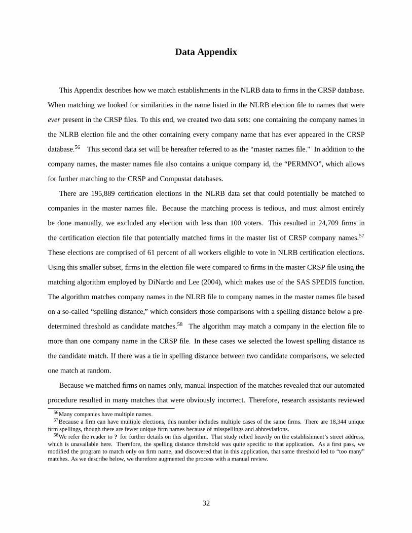
Data Appendix

This Appendix describes how we match establishments in the NLRB data to firms in the CRSP database.

When matching we looked for similarities in the name listed in the NLRB election file to names that were

ever present in the CRSP files. To this end, we created two data sets: one containing the company names in

the NLRB election file and the other containing every companyname that has ever appeared in the CRSP

database.56 This second data set will be hereafter referred to as the “master names file." In addition to the

company names, the master names file also contains a unique company id, the “PERMNO”, which allows

for further matching to the CRSP and Compustat databases.

There are 195,889 certification elections in the NLRB data set that could potentially be matched to

companies in the master names file. Because the matching process is tedious, and must almost entirely

be done manually, we excluded any election with less than 100voters. This resulted in 24,709 firms in

the certification election file that potentially matched firms in the master list of CRSP company names.57

These elections are comprised of 61 percent of all workers eligible to vote in NLRB certification elections.

Using this smaller subset, firms in the election file were compared to firms in the master CRSP file using the

matching algorithm employed by DiNardo and Lee (2004), which makes use of the SAS SPEDIS function.

The algorithm matches company names in the NLRB file to company names in the master names file based

on a so-called “spelling distance,” which considers those comparisons with a spelling distance below a pre-

determined threshold as candidate matches.58 The algorithm may match a company in the election file to

more than one company name in the CRSP file. In these cases we selected the lowest spelling distance as

the candidate match. If there was a tie in spelling distance between two candidate comparisons, we selected

one match at random.

Because we matched firms on names only, manual inspection of the matches revealed that our automated

procedure resulted in many matches that were obviously incorrect. Therefore, research assistants reviewed

56Many companies have multiple names.57Because a firm can have multiple elections, this number includes multiple cases of the same firms. There are 18,344 unique

firm spellings, though there are fewer unique firm names because of misspellings and abbreviations.58We refer the reader to? for further details on this algorithm. That study relied heavily on the establishment’s street address,

which is unavailable here. Therefore, the spelling distance threshold was quite specific to that application. As a first pass, wemodified the program to match only on firm name, and discoveredthat in this application, that same threshold led to “too many”matches. As we describe below, we therefore augmented the process with a manual review.

32

every match and dropped those where they judged the two firm names as different companies.59,60 We then

collected all of the unmatched companies in the election file, from the initial set of 24,709, and attempted to

locate each one in Dun and Bradstreet’s Million Dollar Directory and the Lexis/Nexis’ Directory of Corporate

Affiliations for the year of election. This step identified subsidiaries of publicly traded parent companies,

and allowed us to spot companies that were dropped erroneously in the previous step.

We ultimately matched 7,693 elections from the NLRB election file to companies in the CRSP master

file. In 1,579 cases, the firm in the CRSP file was not publicly traded at the time of the election. After

excluding the private firms, our final sample contained 6,114elections, consisting of 20 percent of all workers

eligible to vote in NLRB elections.

To determine whether the matches appeared reasonable, we compared the reported two-digit SIC industry

code and the state of the establishment from the election fileto the corresponding variables in the CRSP and

Compustat files, for industry and state respectively. Because companies are diversified, the main SIC code

for a company in the CRSP database need not be the same as the SIC code for a particular establishment in

the NLRB election file. Similarly, an establishment may not be located in the same state as the company’s

headquarters. However, the comparisons are reassuring: the two digit SIC codes in the two data sets are the

same for 50 percent of the matches, while 40 percent of the matches show the same state. For reference,

if we randomly pair companies from the final NLRB data set to companies in the master names file that

were never matched to the NLRB data through our procedure, the corresponding match rate is 5 percent for

industry and 4 percent for state.

59For example, the algorithm determined that any company in the election file with the word “American” as part of its name wasa sufficiently good match for the company “American Enterprises” in the CRSP file, if a better match did not exist. Therefore, a dis-parate set of companies like “American Laundry,”“AmericanEnvelope,”and “Pan American Screws” were all matched to “AmericanEnterprise.”All of these matches were dropped by our research assistants.

60Because there was an element of judgment, these exclusions were recorded in a log file for replication purposes.

33

Figure I

Cumulative stock market returns surrounding National Linen Service’s 1999 representation election

Figure II

Average cumulative returns of union victory firms and of the size-matched reference portfolio, by month relative to NLRB case closure

Note: Union victory firms consist of publicly traded companies holding representation elections where at least 5% of the company’s workforce voted, and where the union won. Each point is the average cumulative return up to the month relative to case closure, beginning 24 months prior to case closure. Each firm in the sample is associated with a benchmark portfolio matched on size. The benchmark series corresponds to the average cumulative return of these size-matched reference portfolios. Returns are expressed net of the risk-free rate.

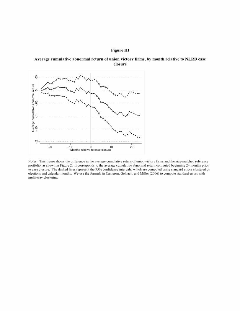
Figure III

Average cumulative abnormal return of union victory firms, by month relative to NLRB case closure

Notes: This figure shows the difference in the average cumulative return of union victory firms and the size-matched reference portfolio, as shown in Figure 2. It corresponds to the average cumulative abnormal return computed beginning 24 months prior to case closure. The dashed lines represent the 95% confidence intervals, which are computed using standard errors clustered on elections and calendar months. We use the formula in Cameron, Gelbach, and Miller (2006) to compute standard errors with multi-way clustering.

Figure IV

Average cumulative returns of union loss firms and of the size-matched reference portfolio, by month relative to NLRB case closure

Note: Union loss firms consist of publicly traded companies holding representation elections where at least 5% of the company’s workforce voted, and where the union lost. Each point is the average cumulative return up to the month relative to case closure, beginning 24 months prior to case closure. Each firm in the sample is associated with a benchmark portfolio matched on size. The benchmark series corresponds to the average cumulative return of these size-matched reference portfolios. Returns are expressed net of the risk-free rate.

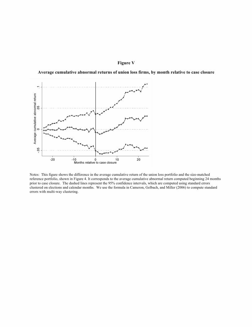
Figure V

Average cumulative abnormal returns of union loss firms, by month relative to case closure

Notes: This figure shows the difference in the average cumulative return of the union loss portfolio and the size-matched reference portfolio, shown in Figure 4. It corresponds to the average cumulative abnormal return computed beginning 24 months prior to case closure. The dashed lines represent the 95% confidence intervals, which are computed using standard errors clustered on elections and calendar months. We use the formula in Cameron, Gelbach, and Miller (2006) to compute standard errors with multi-way clustering.

Figure VI

Average cumulative abnormal return, by analyst coverage

Note: A company is considered to have analyst coverage if it appears in the I/B/E/S dataset in the year of the election. The sample is limited to elections occurring in years where I/B/E/S data were available, between 1976 and 1999

Figure VII

Cumulative abnormal returns in the two years after NLRB closes election, by relation to vote share

Note: Abnormal returns are the simple difference in the security’s return and the size-matched benchmark portfolio in the same month. Cumulative abnormal returns are the sum of the abnormal returns over a two year period beginning in the month of case closure. Predicted values are calculated using a sixth-order polynomial, and an indicator for whether the union won. Dashed lines are the 95% confidence interval. Dots are the average cumulative excess return in 20 equally spaced bins. See Section 4.4 for further details on the construction of this figure.

E[CA

R(0,24

)|Union

 vote  share]  

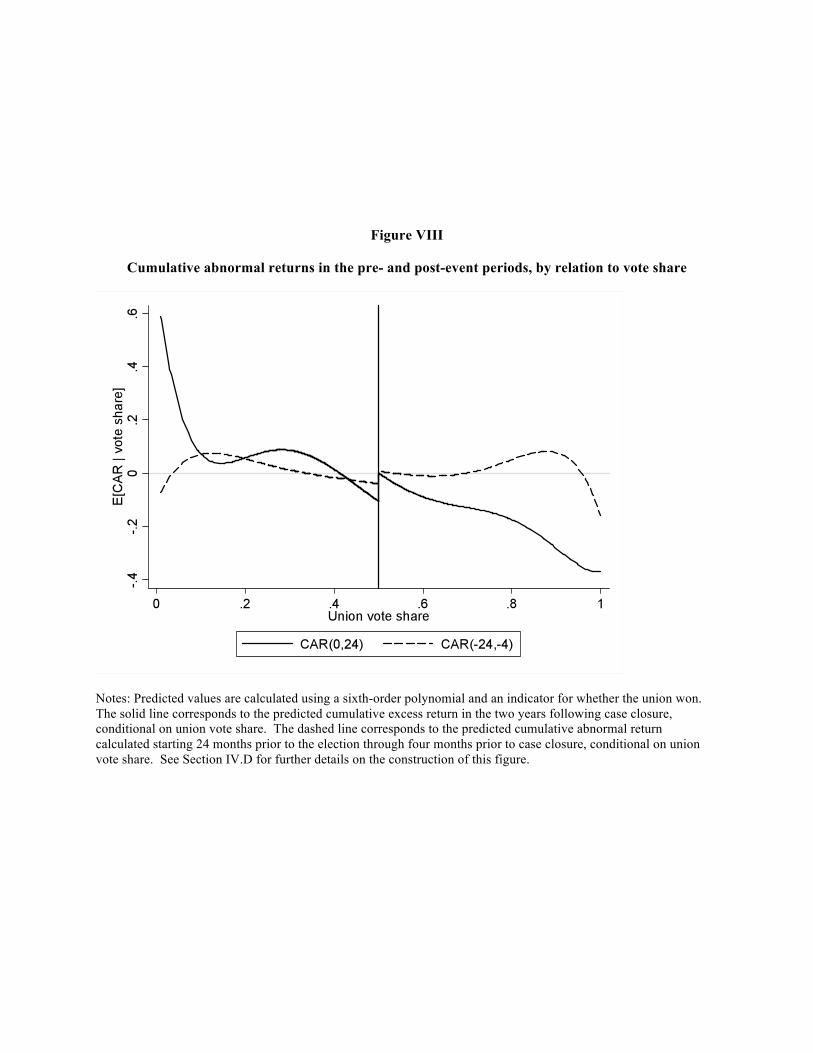
Figure VIII

Cumulative abnormal returns in the pre- and post-event periods, by relation to vote share

Notes: Predicted values are calculated using a sixth-order polynomial and an indicator for whether the union won. The solid line corresponds to the predicted cumulative excess return in the two years following case closure, conditional on union vote share. The dashed line corresponds to the predicted cumulative abnormal return calculated starting 24 months prior to the election through four months prior to case closure, conditional on union vote share. See Section IV.D for further details on the construction of this figure.

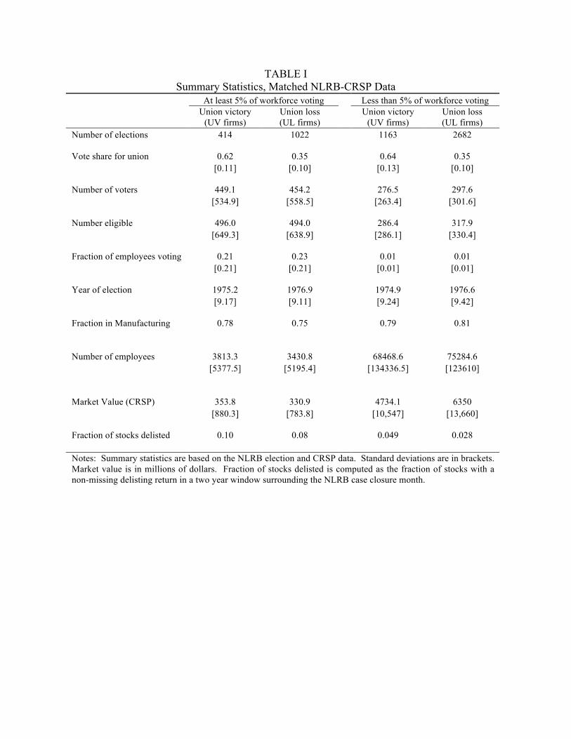
TABLE I Summary Statistics, Matched NLRB-CRSP Data

At least 5% of workforce voting Less than 5% of workforce voting

Union victory

(UV firms) Union loss (UL firms)

Union victory (UV firms)

Union loss (UL firms)

Number of elections 414 1022 1163 2682 Vote share for union 0.62 0.35 0.64 0.35 [0.11] [0.10] [0.13] [0.10] Number of voters 449.1 454.2 276.5 297.6 [534.9] [558.5] [263.4] [301.6] Number eligible 496.0 494.0 286.4 317.9 [649.3] [638.9] [286.1] [330.4] Fraction of employees voting 0.21 0.23 0.01 0.01 [0.21] [0.21] [0.01] [0.01] Year of election 1975.2 1976.9 1974.9 1976.6 [9.17] [9.11] [9.24] [9.42] Fraction in Manufacturing 0.78 0.75 0.79 0.81 Number of employees 3813.3 3430.8 68468.6 75284.6 [5377.5] [5195.4] [134336.5] [123610] Market Value (CRSP) 353.8 330.9 4734.1 6350 [880.3] [783.8] [10,547] [13,660] Fraction of stocks delisted 0.10 0.08 0.049 0.028 Notes: Summary statistics are based on the NLRB election and CRSP data. Standard deviations are in brackets. Market value is in millions of dollars. Fraction of stocks delisted is computed as the fraction of stocks with a non-missing delisting return in a two year window surrounding the NLRB case closure month.

TABLE II

Estimates of post-election cumulative abnormal returns (1) (2) (3)

Size-matched benchmark

Size × industry-matched benchmark

Broad-market benchmark

Panel A: Union Victory ACAR(0,24) -0.092 -0.096 -0.103 (0.028) (0.028) (0.029) ACAR (-24,-4) -0.010 -0.009 -0.010 (0.020) (0.020) (0.020) Panel B: Union Loss ACAR (0,24) 0.029 0.020 0.016 (0.021) (0.020) (0.022) ACAR (-24,-4) 0.034 0.004 -0.009 (0.022) (0.014) (0.014) Notes: ACAR(X,Y) denotes the average cumulative abnormal return from month X to month Y relative to the NLRB case closure month. There are 414 elections in the sample in Panel A, and 1022 elections in Panel B. See Section III.B for details on the construction of the benchmark portfolios and estimation.

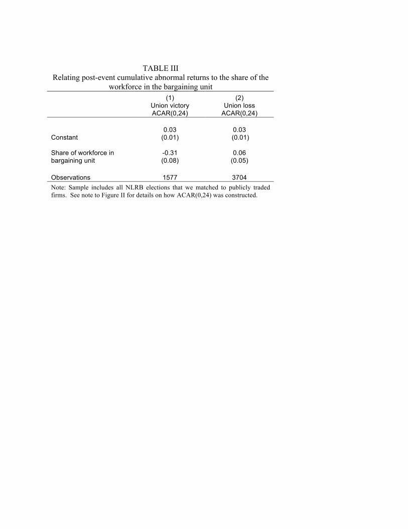
TABLE III Relating post-event cumulative abnormal returns to the share of the

workforce in the bargaining unit

(1) Union victory ACAR(0,24)

(2) Union loss

ACAR(0,24)

Constant 0.03

(0.01) 0.03

(0.01) Share of workforce in bargaining unit

-0.31 (0.08)

0.06 (0.05)

Observations 1577 3704 Note: Sample includes all NLRB elections that we matched to publicly traded firms. See note to Figure II for details on how ACAR(0,24) was constructed.

TABLE IV Evaluation of Arbitrage Strategies

Arbitrage Strategy Buy and Hold Benchmark

Event Month Coefficient of

Variation Percent Positive Coefficient of

Variation Percent Positive Panel A: Individual Investor Strategy 5 0.211 0.606 0.398 0.664 10 0.226 0.633 0.629 0.737 15 0.215 0.647 0.737 0.773 Panel B: Diversified Strategy 5 0.209 0.595 0.426 0.668 10 0.313 0.620 0.603 0.718 15 0.377 0.678 0.746 0.775 24 0.427 0.695 0.958 0.844 36 0.497 0.674 1.113 0.879 60 0.604 0.780 1.231 0.941 120 0.867 0.802 1.382 1.000 360 2.829 1.000 4.458 1.000 Notes: Panel A provides the coefficient of variation of the returns, and the percent of the time the returns are positive for 414 investors. In the first two columns, each investor follows a zero-investment portfolio, holding a short position in the UV firm and a long position in its benchmark portfolio. In the second two columns, the CRSP stock index is held instead. Panel B provides the same statistics for a single diversified investor (as described in the text) over all possible starting months within the sample period.

TABLE V Cumulative abnormal returns in relation to vote share

CAR(0,24): CAR(-24,-4): (1) (2) (3) (4) (5) (6) (7) (8) Constant 0.029 -0.065 -0.075 -0.064 0.0003 -0.018 -0.029 -0.035 (0.021) (0.030) (0.039) (0.035) (0.016) (0.025) (0.033) (0.030) Union victory -0.121 0.048 0.080 0.049 0.003 0.037 0.021 0.027 (0.035) (0.054) (0.066) (0.053) (0.028) (0.046) (0.057) (0.047) Union victory -0.016 0.332 ×vote share (0.321) (0.255) vote share -0.616 -0.610 -0.123 -0.235 (0.160) (0.207) (0.126) (0.162) p(vote share) X X Observations 1436 1436 1436 1436 1436 1436 1436 1436 Note: Robust standard errors are in parentheses. The sample consists of all elections where at least 5% of the workforce voted. The variable “vote share” denotes the union vote share, minus 0.5. Following Dinardo and Lee (2004), the vote share is aggregated to 20 discrete bins. The dependent variable is the cumulative abnormal return from months 0 to 24 relative to case closure (columns 1-4), and the cumulative abnormal return from -24 through -4 months relative to case closure (columns 5-8). The term p(vote share) denotes a fourth-order polynomial in the union vote share.