Embed Size (px)
Citation preview
Long-run seasoned-equity offering returns:
Data snooping, model misspecification, or mispricing?
A costly arbitrage approach*
Jeffrey Pontiff University of Washington
School of Business, Box 353200 Seattle, WA 98119
Michael J. Schill The A. Gary Anderson Graduate School of Management
University of California Riverside, CA 92521
First Draft: February 28, 2001
This Draft: May 10, 2001
Abstract
This paper uses a new approach to assess return behavior after seasoned equity offerings. Our approach recognizes that sophisticated investors are motivated to correct mispricing, although the magnitude of their activity is influenced by arbitrage costs. This approach avoids inference problems due to model misspecification or data snooping. The evidence supports the contention that firms that conduct seasoned equity offerings are overpriced. Our findings imply that, since mispricing associated with seasoned equity offerings is persistent in the long-run, holding costs play an important role although transaction costs do not. In fact, holding costs dominate the size effect documented by previous research.
* We are grateful to Wayne Ferson, Ed Rice, and seminar participants at Emory University and the University of California -Riverside for useful comments and to Larry DuCharme for data assistance.
1
1. Introduction
Whether or not financial markets are efficient has been a long standing subject of debate
(Keynes, 1936, and Friedman, 1953). Testing market efficiency has always been problematic.
First, as Fama (1976) points out, any test of market efficiency is also a test of an asset pricing
model. Because of this, rejection of the null hypothesis may imply that either markets are
inefficient or the model is wrong. Second, rejection of the null may occur when the null is true
(Type I error). Various data snooping biases will produce disproportional large Type I errors.
Both of these problems make interpretation of abnormal stock returns problematic.
Recently, researchers have documented poor performance of long-run stock returns
following equity offerings. For example, Loughran and Ritter (1995) find that in the three years
following a seasoned equity offering (SEO), the average abnormal return for issuing firms is
-33%. These findings have been criticized by Fama (1998), who argues that the abnormal returns
detected by long-run performance studies are highly sensitive to the selected model of expected
returns. This sensitivity is demonstrated by Brav et al. (2000) and Mitchell and Stafford (2000),
who show that offerings do not exhibit abnormal performance relative to some benchmarks.
Loughran and Ritter (2000) argue, however, that the benchmarks selected by Brav et al. and
Mitchell and Stafford incorporate mispricing proxies rather than true risk factors. Thus,
Loughran and Ritter claim that by including mispricing proxies as benchmarks, these studies bias
the test against finding abnormal performance when it exists. The debate between proponents
and detractors of market efficiency stems from the fact that the "true" equilibrium asset pricing
model is unknown to the researcher, and it is impossible to distinguish between mispricing and
model misspecification.
Disentangling identification between mispricing and model misspecification is important
for understanding firms’ decisions to issue equity. If the stock of firms, which conduct SEOs, is
overpriced, the decision to issue equity can be viewed as an opportunity to create value for old
shareholders by selling overpriced or “frothy” shares to new shareholders [see, Loughran and
Ritter (2000) and Schill (2000)]. In an efficient market this transaction does not generate
systematic gains, since efficiency implies that after the SEO announcement, the stock price is
fairly valued, negating any systematic benefit from the offering [Myers and Majluf (1984)]. In
the case of market efficiency, lower post-SEO returns reflect equilibrium asset pricing. This may
be attributable to a lower cost of capital, perhaps due to decreased exposure to an unknown type
of priced risk [Eckbo, Masulis, and Norli (2000)].
2
Our paper uses a completely different methodology to study long-run SEO performance.
Specifically, our test largely avoids the abnormal return/model misspecification joint hypothesis
problem as well as data snooping biases. We acknowledge that mispricing creates profit
opportunities for sophisticated investors who act as arbitrageurs. The trading behavior of these
investors creates price impact that decreases the equilibrium amount of mispricing. In a
frictionless market, arbitrageurs eliminate all pricing error. In a world with non-zero market
friction, mispricing can persist since various costs impede the profits of arbitrageurs [for example,
Shleifer and Vishny (1990, 1997) and Pontiff (1996)]. Since the costs that affect arbitrageurs
vary depending on security type and market conditions, mispricing can be greater when these
costs are greater, and smaller when these costs are smaller. Since our approach makes predictions
regarding the relation between mispricing and arbitrage costs, it provides a rejectable test of
market efficiency.
Our approach is similar to Pontiff (1996) who shows, cons istent with mispricing, that the
magnitude of the deviation between closed-end fund prices and net asset values is greater for
funds with higher arbitrage costs. Two differences separate our tests from Pontiff. First,
Pontiff’s test includes both overpriced and underpriced securities. Since the SEO debate concerns
whether managers time overvaluation, our test focuses on overvaluation. Second, Pontiff has a
direct measure of mispricing--closed-end fund discounts, which is the deviation between closed-
end fund prices and net-asset values, whereas we must infer mispricing from ex-post SEO stock
performance.
Our study varies from previous studies of arbitrage costs and performance in two
important ways. First, virtually all studies, with the exception of Pontiff (1996) and Karpoff and
Walking (1990), compare abnormal returns with transaction costs and make conclusions based on
whether or not the transactions costs are large enough to make arbitrage unprofitable.1 The
intention of this vast literature is to address whether or not an apparent market inefficiency
implies profit opportunities. Our study does not attempt to address this question. We avoid this
question since total arbitrage costs are difficult to measure and the notion of “profit” depends on
which costs the arbitrage investor considers sunk. Rather we appeal to the notion that, all
1 For example, the relation between abnormal returns and transaction costs has been investigated by Fama and Blume (1966) for filter rules, Jensen and Benington (1970) for portfolio upgrading rules, Dann et al. (1977) for block-trade returns, Phillips and Smith (1980) for option trading rules, Bhardwaj and Brooks (1992) and Reinganum (1983) for the January effect, Stoll and Whaley (1983) for the small-firm effect, Mech (1993) and Knez and Ready (1996) for switching strategies, Pontiff (1995) for closed-end fund trading strategies, Lesmond (2000) for post-earnings price drift, Copeland and Mayers, (1982), Barber et al. (2000), and Choi, (2000) for analyst recommendation underreaction, and Lesmond et al. (2001) for momentum trading returns.
3
arbitrage trades have zero marginal profit. This notion is common to all models (behavioral or
otherwise) that include arbitrage by economically rational agents.
Second, our paper uses a broad definition of arbitrage costs, which includes both
transaction costs and holding costs. Although theoretical literature frequently incorporates
holding costs [for example, Shleifer and Vishny (1990), De long et al. (1990), and Tuckman and
Vila (1992)], the empirical literature, with the exception of Pontiff (1996), has not. As we will
show, holding costs are the key arbitrage cost that affect SEO long-run returns.
In summary, our results are consistent with SEOs being overpriced. Arbitrage costs are
related to poor post-SEO stock performance. The holding costs associated with SEO arbitrage
appear particularly important in explaining cross-sectional performance. Overall, the cross-
sectional variation in one-time transaction costs associated with SEO arbitrage has little effect on
long-run mispricing. We find that holding costs dominate the previously documented size effect
of long-run equity offering performance [Brav and Gompers (1997)].
Section 2 discusses the mechanics of costly arbitrage, as well as a detailed description of
the impact of transaction costs and holding costs. Section 3 discusses statistical inference in light
of model misspecification. Section 4 describes the data used in the study as well as the
computation of return performance measures. Section 5 discusses the cross-sectional estimation
results. Section 6 explores whether inference may be hampered by universal relations between
arbitrage costs and stock returns. Section 7 discusses the time-series estimation results. Section 8
concludes.
2. Mispricing and Arbitrage Costs
For an undervalued security classic costless arbitrage involves costlessly buying shares of
the security and costlessly selling a fair-priced security that is perfectly correlated with the
fundamental value of the undervalued security. For an overvalued security, arbitrage involves
costlessly selling the overvalued stock and costlessly buying a fair-priced security that is perfectly
correlated with the fundamental value of the overpriced security. The arbitrageur then costlessly
holds this position until prices reflect fundamental values. These strategies make the arbitrage
4
risk-free. In practice, this arbitrage is not possible since trading is costly, holding positions are
costly and require capital, and it is difficult to perfectly hedge a position.
Arbitrage costs directly affect the ability of sophisticated traders to reduce mispricing.
Specifically, two types of costs affect arbitrage profits: transaction costs and holding costs.
Transaction costs are incurred when positions are opened or closed, whereas holding costs are
incurred every period that the position is held. Mispricing may be more severe for assets that are
more costly to arbitrage since these assets are subject to weaker corrective arbitrage pressure.
Following Pontiff (1996), this section analyzes these costs and their relation to mispricing.
Transaction costs pose an obvious barrier to arbitrage. These costs are incurred per
transaction, and include brokerage fees, market impact costs, and bid-ask spreads. Transaction
costs exhibit substantial cross-sectional variation (for example, Stoll and Whaley, 1983; Kothare
and Laux, 1995; Knez and Ready, 1996; Chan and Lakonishok, 1997; Jones and Seguin, 1997;
and Lesmond et al., 1999). In a mispricing equilibrium that only involves transaction costs, the
arbitrage trades of an economically-rational investor will yield the same net return regardless of
transaction costs. Thus, for securities with larger transaction costs, arbitrage pressure will only
take place at larger magnitudes of mispricing. Securities with high transaction costs can maintain
higher mispricing in equilibrium than securities with lower transaction costs. Garman and Ohlson
[1981] generalize the implications of arbitrage pricing when market participants face transaction
costs. They show that the arbitrage-implied price of an asset in the presence of transaction costs
is simply the arbitrage-implied price of the asset in the absence of transaction costs, plus or minus
a discrepancy that they call a “fudge factor.” The magnitude of this discrepancy is directly
related to the size of the transaction costs.
Holding costs are incurred every period the arbitrage position is held. Examples of
holding costs include borrowing costs, opportunity costs from not being able to fully invest short-
sale proceeds, and risk exposure from imperfectly hedged positions. Shleifer and Vishny [1990]
and Tuckman and Vila [1993] examine an investor's willingness to engage in arbitrage when
confronted with holding costs. Mispricing in equilibrium is greater in longer-term versus shorter-
5
term assets, since arbitrage in the former involves incurring holding costs over more periods.
Tuckman and Vila show that holding costs cause even perfectly hedged arbitrage positions to be
risky, since losses will be incurred if the mispricing does not dissipate quickly enough. Thus,
similar to De Long et al. [1990], mispricing risk induces the risk-averse arbitrageur to hold a
finite arbitrage position.
To some extent, an arbitrageur will assess tradeoffs between transaction costs and
holding costs. This is important since creating a hedge involves costly transactions. Thus, the
arbitrageur may choose to economize on transaction costs by bearing greater holding costs.
Forgone interest is an important holding cost. Due to margin requirements, traders are
not able to invest the full proceeds of their short sales, although large traders are sometimes able
to negotiate a rebate for forgone interest. Because a competitive interest rate is earned on only a
fraction of the withheld proceeds (a typical agreement states that the trader receives the brokers'
call rate on 75 percent of the short-sale proceeds), interest rates are related to the opportunity cost
of the short sale.
If the arbitrageur cannot perfectly hedge the fundamental value of the arbitrage position,
then arbitrage involves risk. For typical stocks, fundamental value can be hedged with portfolios
that are sensitive to the company’s fundamental performance. In the case of fundamental value
that is related to the value of the market portfolio, securities that are meant to approximate the
market portfolio can be used as hedges. In any case, unhedgeable fundamental risk imposes a
cost.
Dividend payments reduce holding costs by reducing the amount of capital that must be
devoted to the arbitrage position in future periods. Although the security is subject to mispricing,
the dividend is not, i.e., when the dividend is paid investors receive the full value of the dividend,
regardless of mispricing. Each time a dividend is paid, a partial liquidation of the mispriced
security occurs. Holding costs are related to the size of the position, so dividends reduce the
amount of capital that is subject to holding costs. In the extreme case of a liquidating dividend,
the arbitrageur only expects to incur holding costs for the periods before the dividend. In
6
equilibrium, securities that pay large dividends will be subject to less mispricing since the holding
costs incurred by arbitrageurs are smaller.
3. A costly arbitrage test for abnormal returns.
We motivate our empirical methods with a simple model of returns. An equilibrium
model determines expected returns in the absence of mispricing. The model is bifurcated into
two parts, C1 and C2. C1 is the part of the model that the researcher uses to calculate expected
returns. C2 is not known, and thus not utilized by the researcher. Conceptually, we can think of
C2 as being undiscovered factors that complete the asset pricing model. Realized returns are
comprised of three components, mispricing, M, an expected return component that is dictated by
the true equilibrium model, C1+ C2, and noise, e1. e1 is assumed to be uncorrelated to M, C1, and
C2. If M is positive (negative) the security is underpriced (overpriced) and is expected to have an
abnormally high (low) return. The return of the security, r, can be expressed as,
121 eCCMr +++= (1)
Mispricing is comprised of two multiplicative effects, η , which is related to the expected
return bias of irrational traders, and A , which reflects arbitrage costs.
AM η= (2)
No arbitrage costs imply no mispricing. Although arbitrage costs do not influence
whether the mispricing is positive or negative, the magnitude of potential mispricing
increases in arbitrage costs. A security with a negative (positive) η is likely to have
negative (positive) future returns, and is overpriced (under priced).
Besides not using the entire equilibrium model of expected returns, the researcher
measures C1 with error. Thus, the researcher’s estimate of expected returns is given by,
21 eCP += (3)
The researcher estimates abnormal returns by subtracting the actual return (1) from the
expected return proxy (3), yielding,
212 eeCAPr −++=− η (4)
The formulation of (4) illustrates the source of Fama’s joint hypothesis problem. The abnormal
return proxy contains a mispricing component, Aη , and a model misspecification component,
7
2C . Observing the level of the abnormal return proxy, ,Pr − does not allow the researcher to
discern between model misspecification and abnormal returns.
Data snooping biases can influence statistics that are based on the abnormal return proxy.
In general, these biases will occur if conditional on information available when the statistics are
calculated, the expectation of 1e is not equal to zero. In the case of post-SEO poor return
performance, a possibility is that instead of having negative returns due to mispricing
)0( 2 <Aησ , firms with SEO have performed poorly due to poor luck—negative 1e . Studies that
use the same data will find the same poor performance.
Our test of mispricing involves the covariance between the abnormal return estimate and
arbitrage costs. If arbitrage costs are uncorrelated to the noise in the researcher’s return forecast,
e2, then this covariance between the abnormal return estimate and arbitrage costs can be written
as,
),(),( 22 ACCovAPrCov A +=− ησ (5)
where 2Aσ is the variance of the arbitrage costs. A test of whether the security is overpriced is a
test of whether 0),( <− APrCov , versus the null hypothesis of 0),( =− APrCov . This test
is uninfluenced by 1e , thus inference is unhampered even if the level of the abnormal return is
influenced by data snooping.
If Cov(C2,A)<0, then this test might lead us to falsely reject null. Fortunately, this
scenario is unlikely, since this would imply that securities that are associated with higher
arbitrage costs have lower expected returns. Most transaction cost models, such as Amihud and
Mendelsohn (1986) predict the opposite. In this case, where Cov(C2,A)>0, the test will still be
well-specified although it will have less power, in that it will fail to reject the null more often than
if C2 were orthogonal to arbitrage costs. Our tests of the mispricing of SEOs center on testing this
implication.
4. Data
Our sample of offerings includes all primary U.S. common seasoned equity offerings
from the Securities Data Company (SDC) Global New Issues dataset from January 1970 to
December 1995. The SDC sample is composed almost exclusively of firm-commitment
offerings, which generally eliminates the smaller, speculative, "penny" stock best-efforts issues.
8
The sample also excludes equity carve-outs. As in Loughran and Ritter (1995), all regulated
utility issuers (SIC code 481 before 1985, 491-494), closed-end funds (SIC code 672-673), real
estate investment trusts (SIC code 6798), and American Depository Receipts are excluded from
the sample due to the unique nature of their offerings and the equity issue restrictions they face.
We also require offering firms to be listed on the Center for Research in Security Prices (CRSP)
database prior to the offering.
4.1 Long-run performance
A host of models have been used in the literature to determine long-run new offering
return performance. Ritter (1991) introduced the control firm buy-and hold return measure. This
measure has been adopted widely using different attributes by which to select control firms,
including size (Loughran and Ritter, 1995); size and book-to-market (Brav and Gompers, 1997,
Jegadeesh, 2000, and Brav et al., 2000); size and industry (Spiess and Affleck-Graves, 1995);
and size, book-to-market, momentum, price, and dividend yield (Jegadeesh, 2000). Fama (1998)
advocates the alternative use of factor models to compute cumulative average returns. Loughran
and Ritter (1995), Brav and Gompers (1997), and Mitchell and Stafford (2000) use the Fama-
French three factor model. Brav et al. (2000) use variations of the Fama-French three-factor
model and Carhart's four-factor variation. Eckbo et al. (2000) use a model with six
macroeconomic risk factors to price equity offerings.
Given the wide range of model preferences and the difficulty in distinguishing risk
factors from mispricing proxies, we measure long-run performance using three "plain vanilla"
models: the Capital Asset Pricing Model (CAPM), the standard three factor Fama-French model,
and the size-matched control firm approach. For each model, we measure performance over
calendar months t+1 to t+36, which has been shown to comprise the bulk of new issue
underperformance (see Loughran and Ritter, 1995).
CAPM abnormal performance for firm i is defined as,
)(36
1∑
=
−t
mtiit rbr (6)
where rit is the monthly return for firm i less the Treasury Bill yield t months after the offering,
rmt is the monthly return for the CRSP value-weighted market less the Treasury Bill yield t
months after the offering. bi is an estimate of firm i’s beta, which is computed from a regression
9
of excess market return on the excess return of the CRSP. The estimation regression is computed
using available data in the 36 months following the SEO. For firms with less than 6 monthly
observations, bi is set to the sample mean.
The Fama-French 3 factor abnormal return is defined as,
)(36
1∑
=
−−−t
tHMLit
SMBimt
mktiit HMLbSMBbrbr (7)
where SMBt is the monthly small-minus-big size Fama-French factor t months after the offering,
HMLt is the monthly high-minus-low book-to-market Fama-French factor t months after the
offering. For firms with a year or less of post SEO return data, the Fama-French abnormal return
is set identical to the CAPM abnormal return measure.
The size-matched abnormal return is defined as,
36 36
1 1
(1 ) (1 )it
cit
t t
r r= =
+ − +∏ ∏ (8)
where citr is the month t return for a non-issuing control firm that is size-matched with firm i.
This estimation procedure is identical to that of Loughran and Ritter (1995).
4.2. Independent variables
Transaction cost proxies. Reliable explicit estimates of transaction costs are difficult to
obtain prior to the late 1980s (Keim and Madhavan, 1998). We use three proxies for transaction
costs that are available throughout our 26 year sample period. Lesmond et al. (1999) use the
limited dependent variable (LDV) model of Tobin (1958) and Rosett (1959) to estimate round-
trip transaction costs using only the distribution of daily returns. For our sample, the LDV
estimate is obtained using the daily returns of the issuing firm returns in the calendar year prior to
the equity offering. 2 For the small number of firms where sufficient daily return data is not
available we use the coefficients from a regression of the LDV estimates from the respective
decade on the logarithm of firm market capitalization and five share price binary variables for the
respective price ranges of less than $5, $5 to $10, $10 to $15, $15 to $20, and above $20
2 We thank David Lesmond for generously providing the LDV estimates for our sample.
10
following Bhardwaj and Brooks (1992) to estimate the LDV estimate using the firm price and
size values. We apply those coefficients to the SEO's respective size and price to obtain a quasi
LDV estimate for the observations lacking the standard LDV estimate.
We also use the inverse of the firm's stock price at the end of the calendar offering month
(1/P) to proxy for trading costs following Karpoff and Walking (1988). Bhardwaj and Brooks
(1992) find that the average bid-ask spread for stocks with prices under $5 are 6%, while stocks
with prices above $20 have, on average, spreads of 0.9%. Our hope is that the inverse of stock
price captures variation which is similar to bid-ask spread variation. Lastly, the logarithm of
market equity value is used as an alternative transaction-cost proxy because small stocks suffer
from greater illiquidity, spread, short selling constraints, and market impact costs [see, for
example, Stoll and Whaley (1983)].
Holding cost proxies. The risk of an arbitrage position is the volatility of the difference
between the mispriced asset's return and the hedge asset's return. If the arbitrage is perfect, then
the asset's return and the hedge are perfectly correlated, and the arbitrageur is not exposed to any
risk. Finding an appropriate hedge for firms issuing equity is likely to be challenging. We
expect that the least expensive risk for the arbitrageur to hedge is risk that is related to market
movements, beta risk. For each firm with twelve or more months of return data prior to the
seasoned equity offering, we estimate a regression of excess stock return on the excess return of
the Standard and Poors (S&P) 500 index for the 36 months before the offering. We retain the
beta coefficient and the standard deviation of the model error or root mean square error. The
beta is a measure of the market risk that is attributable to the securities risk, and the root mean
square error is a measure of the idiosyncratic risk, which is difficult to hedge. For firms with less
than twelve months of return data before the offering, we examine the returns of other firms in
the same industry. Industries are defined using the same procedure as Fama and French (1997).
To obtain industry estimates, we estimate a regression of stock return on the return of the S&P
500 index for each firm in the industry. We use the average industry beta and root mean square
error estimated over the 36 months prior to the offering as the beta and root mean square error of
the SEO firm.
Returns are comprised of dividend payments and price appreciation. Although prices are
subject to mispricing, dividend payments are not. Because of this, dividend yield is related to the
expected holding period required for an arbitrage position. Each time a dividend is paid the
arbitrage position is partially liquidated. Since arbitrageurs expect to incur greater total holding
costs for positions that they expect to hold longer, ceteris paribus, arbitrageurs will view arbitrage
11
in high dividend yield securities as less costly than low yield securities. For example, a stock
that will pay a liquidating distribution next period will only create holding costs for one period.
Dividend yield is measured as the sum of the dividends paid per share for the 12-month before
the offering, divided by the price level at the time of the offering.
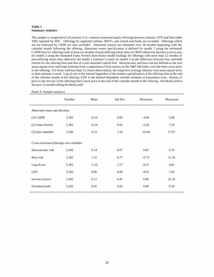
Table 1 provides summary statistics for the sample of 5,303 seasoned equity offerings.
Consistent with previous SEO studies, mean abnormal return estimates are significantly negative
and range from -24 percent for the CAPM model, -14 percent for the Fama-French model, and -
21 percent for the size-matched buy-and-hold model.3 In Panel A, we also report summary
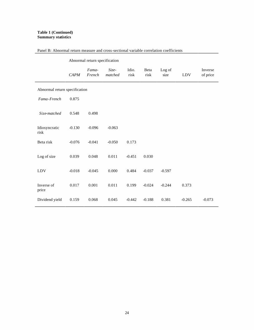
statistics for the cross-sectional and times-series independent variables. Panel B provides
correlation coefficients for the cross-sectional variables. The CAPM and Fama-French abnormal
return estimates are highly correlated with a correlation coefficient of 0.88. The size-matched
abnormal return is less correlated with the other model estimates with coefficient estimates of
0.55 and 0.50 for the CAPM and Fama-French model, respectively. The univariate correlation
between long-run performance and the arbitrage cost proxy variables suggest that mispricing is
bound by the costs of arbitrage as predicted by the arbitrage cost explanation. Larger beta risk
and idiosyncratic risk is associated with worse abnormal performance. Higher dividend yield is
associated with lower mispricing. Long-run performance is also increasing in size and
decreasing in LDV transaction costs as predicted. Only the share price variable produces
correlation coefficients that are inconsistent with univariate predictions.
5. Cross-sectional estimation results
The cross sectional arbitrage cost estimation is presented in table 2. Our estimation
procedure is designed to mitigate problems due to cross correlation in post-SEO returns, as well
as problems associated with heteroskedasticity.
First, individual equity offerings may not represent independent events. Firms that issue
equity contemporaneously are likely to share similar characteristics. Loughran and Ritter (1995)
find that long-run abnormal returns for firms issuing equity during periods of heavy offering
volume tend to perform worse than firms that issue equity during period of light offering volume.
If the statistical test assumes independence, contemporaneous observation correlation is likely to
bias the test (Brav, 2000; Mitchell and Stafford, 2000).
12
Dummy variables based on calendar time may not be useful in correcting for this problem
since if each time period has equal length, variation in the volume of SEO may lead to the
dummy variables that under control for high volume cycles (since too much activity occurs
during a period) and under control for low volume cycle (since too few offerings occur). We
avoid this problem by creating 11 dummy variables that are based on offering time. We separate
our offering dataset into 12 time groups where each group has the same number of offerings.
Because of this, high volume periods have time dummy variables that comprise shorter calendar
periods, whereas lower volume periods have time dummy variable that comprise longer calendar
periods. Overall, we expect this specification does a good job capturing intertemporal variation
in post-SEO returns. As a specification check, we regress firms’ estimation residuals on the
estimation residuals of other firms’ with offerings in the same month. From this test, we are
unable to reject the null hypothesis of no correlation between the abnormal returns for SEOs
during the same month. Although all cross-sectional estimation use 11 cycle dummies, for
presentation reasons, coefficients on the dummy variables are omitted from table 2.
Second, we expect residual heteroskedasticity that is related to firm characteristics as
well the time period. Our approach to this problem is to use a two-pass procedure. A first pass
ordinary least squares regression is estimated. The natural log of the squared residuals from this
regression are used as the dependent variable in an ordinary least squares regression where the
independent variables are; the natural log of firm return variance in the three years before the
SEO, the natural log of the return variance of the CRSP equal weighted index in the three years
following the SEO, the natural log of the firm market capitalization, the LDV transaction cost
measure, the firm’s dividend yield, and the 11 time dummy variables. We chose these variables
since we expect them to be related to the heteroskedasticity that is associated with our abnormal
return measure. The inverse of the exponent of this predicted value of this estimation is used as a
weight in a second-pass weighted least squares regression.
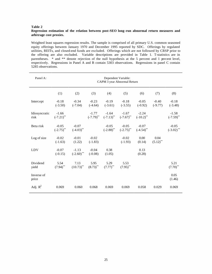
The estimation results are presented in table 2. Panel A reports results using the CAPM
as the appropriate return generating process, panel B reports results using the Fama French three
factor model as the appropriate return generating process, and panel C reports results where
abnormal returns are calculated relative to a size-matched control firm.
Holding cost results. Overall, the three panels offer support to the contention that all
three return specifications produce estimates of abnormal returns and that holding costs are an
3 We are unable to obtain size-matched control firm estimates for 18 SEOs. The omitted firms do not
13
impediment to arbitrage. First, consistent with the hypothesis that idiosyncratic risk is an
arbitrage cost, there is a strong negative relation between idiosyncratic risk and three-year
abnormal returns following SEOs. Thus, firms with higher level of idiosyncratic risk tend to have
more negative abnormal returns following the offering. The null of no relation can be rejected at
the 1% level regardless of the specification.
Surprisingly, beta risk is also negatively related to three-year abnormal returns.
Although, from examination of the t-statistics this finding appears slightly less robust than the
idiosyncratic risk results, the finding is still puzzling, since if market risk can be inexpensively
hedged, we would not expect beta risk to be related to abnormal returns. This result is somewhat
similar to Pontiff (1996), who finds that mispricing as proxied by closed-end fund discounts is
positively related with market risk, although Pontiff is unable to reject the null of no-relation.
One explanation of our finding is that market risk is, in fact, costly to hedge. This issue is further
explored in section 6.
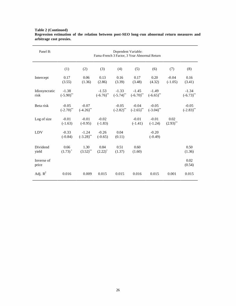
Dividend yield is the proxy for the expected amount of time the arbitrage position is held.
As expected, all specifications produce positive slope coefficients on dividend yield. For the
CAPM specification these results are always significant at the 1% level. For the Fama-French
specification the slope on dividend yield is statistically significant for half the specifications,
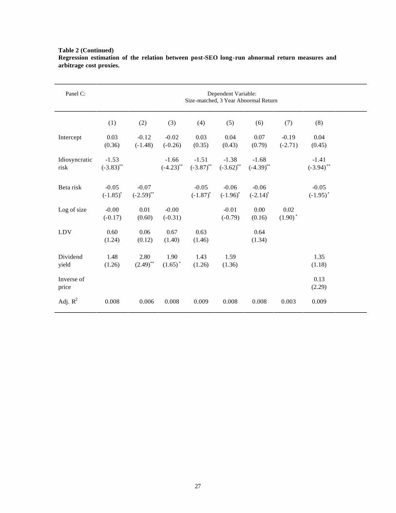
whereas for the size matched specification the slope on dividend yield is only statistically
significant for one specification.
Transaction cost results. We use three proxies for transaction costs; the Lesmond et al
limited dependent variable (LDV) estimate, the natural log of firm size, and the inverse of price.
Overall the slope coefficients on the transaction cost variables either have the opposite sign of
that predicted by costly arbitrage or the slope coefficients are insignificantly different from zero.
From table 1, our transaction costs proxies are highly correlated. Because of this, there is
some value from making inference by comparing estimation when each transaction cost is
included separately (columns 4, 5, and 8). For all three return measures, the sign on the slope of
the transaction cost proxies is opposite of that predicted by costly arbitrage. This finding is
inconsistent with the joint hypothesis that transaction costs are an impediment to arbitrage and
deviations from return generating specifications capture abnormal returns. Given the holding cost
results and the transaction cost results, one interpretation of these results is that, for SEOs,
transaction costs are of second-order importance compared with holding costs. Since the
appear to maintain any specific characteristic bias.
14
abnormal returns associated with SEO take years to dissipate, the finding that the predominant
impediment to arbitrage is holding costs rather than transaction costs has an intuitive appeal.
Column 7 of all three panels demonstrates a positive correlation between size and
abnormal return consistent with Brav and Gompers (1997). On the surface this result appears to
support the costly arbitrage notion of arbitrage with respect to transaction costs, although once
holding cost variables are included this size effect disappears. Thus, the size effect noted by other
authors appears to be a proxy for a holding cost effect.
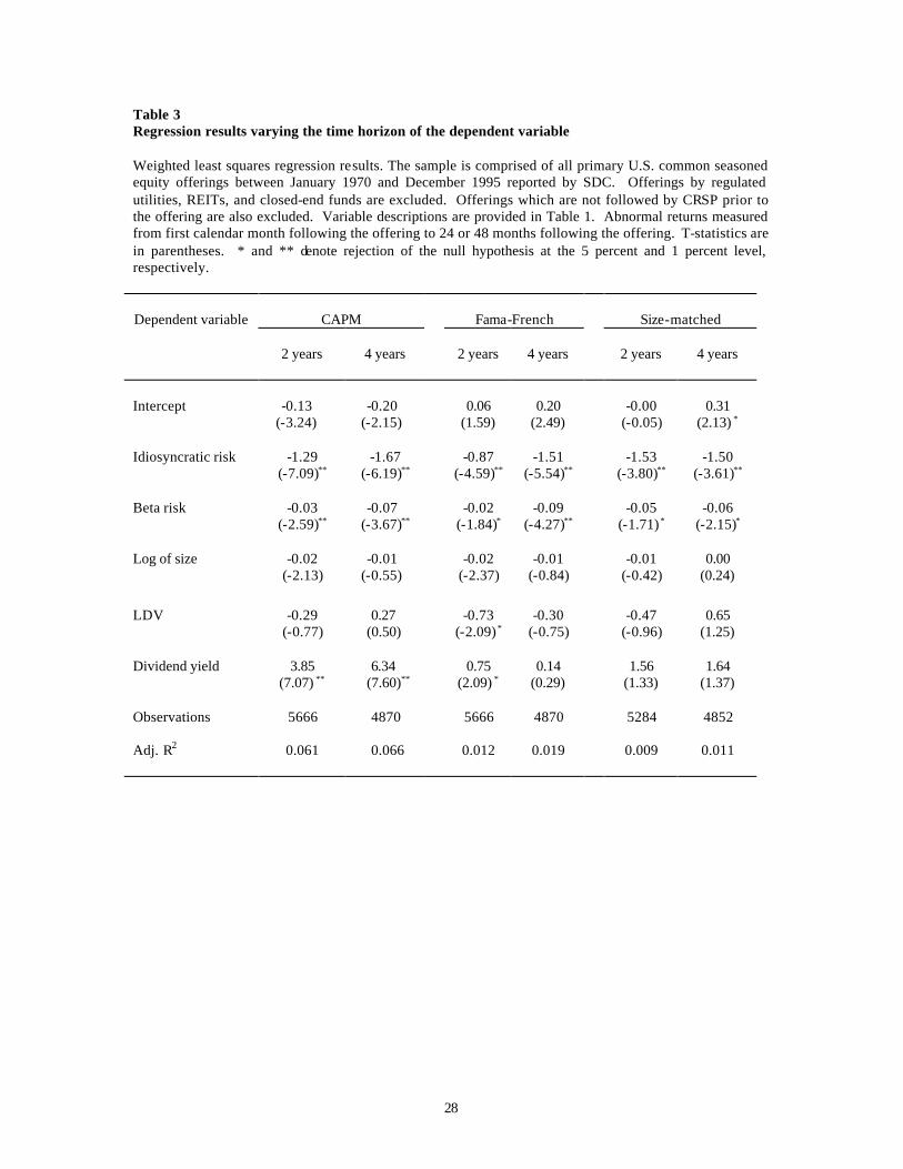
Table 3 investigates the robustness of the table 2 results. Estimation is conducted for two
and four year holding periods. For all estimations, both idiosyncratic risk and beta risk are
always negative and statistically significant. Of these two variables the statistical significance of
idiosyncratic risk is always stronger than beta risk. Dividend yield is always positive, and
statistically significant for the CAPM performance measure but not for the size matched
performance measure. For the Fama-French measure, dividend yield is statistically significant for
two-year performance but not four-year performance. For all specifications, the transaction costs
variables are insignificant except the estimate of the impact of LDV on two-year Fama-French
abnormal returns. The slope is negative, which is consistent with costly arbitrage.
6. Estimating the universal relation between arbitrage costs and abnormal returns
One possible explanation of our results in that our arbitrage costs variables are negatively
related to a portion of the true asset pricing model that is not being captured in our abnormal
return specification. In context of equation 5, this possibility would imply that Cov(C2,A)<0.
Most previous research contradicts the possibility that our arbitrage cost variables will be
negatively correlated with abnormal returns. Malkiel and Xu (1997) for idiosyncratic risk, Banz
(1981) and Reinganum (1981) for size, Amihud and Mendelson (1986) and Brennan and
Subrahmanyam (1996) for transaction costs, and Litzenberger and Ramaswamy (1979) for
dividend yield all find significant positive correlation between returns and the respective arbitrage
cost variables. We recognize that many of these studies do not incorporate long-run returns, nor
do they incorporate the same abnormal return specification that we utilize. Inference may also
me affected by transient relations between arbitrage costs and returns that are evident in our data,
but not in the time periods used by other studies.
In order to address these concerns, we estimate the cross-sectional relationship between
both the CAPM 3 year abnormal return measure and the Fama-French 3-factor abnormal return
15
measure with arbitrage cost proxies. We utilize all stocks on CRSP with December year-end data
between 1969 and 1995, which is the same time period as our SEO sample. Similar to our SEO
estimation, we calculate CAPM abnormal returns for firms with less than 6 months post return
data by using the sample mean beta coefficient of all firms with less than 6 months of data. Also
for firms with less than 12 months of data, the CAPM abnormal return is substituted for the
Fama-French 3-factor return abnormal return. Also similar to the previous SEO estimation, for
firms with less than 12 months of data before December year-end, we utilize the industry average
residual mean square error and S&P beta.
We use a Fama-MacBeth procedure to estimate the cross sectional relation [Fama-
MacBeth (1973)]. Thus, each period a separate regression is estimated. In order to produce
heteroskedastic consistent estimates, each firm is weighted by the inverse of the average absolute
value of its abnormal return in the entire sample. The average slope coefficient from the 26
different annual regressions is reported in Table 4. Since our estimation uses overlapping data,
we utilize standard errors that account for serial dependence.4
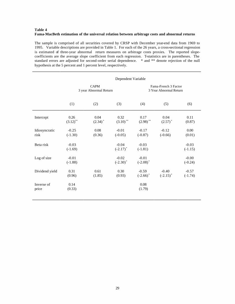
From the results in Table 4, we can not reject the null hypothesis, that the level of
idiosyncratic risk and dividend yield have no ability to predict 3-year CAPM abnormal returns.
Of the three CAPM specifications, the specification that produces a slope coefficient on
idiosyncratic risk that is closest to the SEO cross-sectional results, is column 1 with a slope of
-0.25. The weakest SEO CAPM cross-sectional slope coefficient on idiosyncratic risk is –1.58
(Table 3, Panel A, column 8). The difference between these two coefficients is –1.33,
corresponding to a t-statistic of –4.69 (this t-statistic allows for both slopes to have different
standard errors). Thus, the slope coefficients on idiosyncratic risk in Table 2, panel A, are
significantly more negative than the coefficients from an estimation that utilizes all securities.
This result is consistent with the notion that post-SEO returns reflect over-pricing and that
idiosyncratic risk is a holding cost that impairs the activities of sophisticated traders.
Next, we compare the dividend yield results from the CAPM specifications in Table 4
and Table 2, panel A. The strongest dividend yield slope coefficient from the Fama-Macbeth
regression is 0.6. The weakest dividend yield slope coefficient from Table 2, panel A, is 5.21
(column 8). The difference between these coefficients is 4.60, with a t-statistic of 6.10. This
reaffirms that the Table 2 findings regarding dividend yields are not being driven by market-wide
relations.
4 We estimate a time -series regression of each slope coefficient on an intercept. The residuals from this regression are modeled as a second-order moving average process. The standard error we use to compute
16
The idiosyncratic risk and dividend yield conclusions are roughly similar when we focus
on the Fama-French 3 year abnormal returns. The most negative idiosyncratic risk slope from the
Fama-MacBeth regressions (column 4) is –0.17, whereas the least negative idiosyncratic risk
slope in Table 2, Panel B, is –1.33. The difference between these slope is –1.16, with a
statistically significant t-statistic of –3.84. The largest Fama-MacBeth slope on dividend yield
-0.40 (column 5), whereas the smallest slope in Table 2, Panel B (column 8) is 0.50. The
difference between these two slope is 0.90, with a t-statistic of 2.18. Again, the results from
estimating the relation between abnormal returns and arbitrage costs on all stocks, does not affect
our inference from the SEO sample.
Interestingly, inference from the Table 2 beta coefficient results is affected by the Table 4
results. From the CAPM abnormal return specification, the most negative slope coefficient on
beta risk is –0.07 (Table 2, panel A, column 6). The least negative beta risk slope on Table 4 is
-0.03 (column 1). The difference between the slope coefficients is –0.04, with a t-statistic of
-1.81. From the Fama-French abnormal return specification, the most negative slope on beta risk
is –0.07 (Table 2. panel B, column 2). The least negative beta risk slope in Table 4 is –0.03
(column 6). The difference between these coefficients is –0.04, with a t-statistic of –1.38. To the
extent that beta risk is costless to hedge, the Table 2 estimation should have exhibited no relation
between beta and abnormal returns. The Table 4 findings seem to imply that the contradictory
Table 2 results may be attributed to a market-wide relation between beta and abnormal returns.
7. Time -series estimation results
The impact of interest rates on post-SEO performance cannot be estimated using cross-
sectional techniques, necessitating a time-series test. We conduct a time-series test by computing
the average three-year post SE0 performance for all offerings in a given month. This variable is
used as our dependent variable in our regressions. The 30-day T-Bill yield, aggregate SEO
volume as a fraction of total market capitalization, and a dummy for the month of January are
used as independent variables. SEO volume is used to control for post-offering performance that
is attributable to cycles in the equity market. Our inclusion of this variable is motivated by
Loughran and Ritter (1995) who show that SEO volume is negative correlated with post-SEO
the t-statistics from the Fama-MacBeth estimation is the standard error on the intercept of the time -series regression.
17
performance. As a robustness check, a dummy variable for January has been included since
some anomalous return behavior can be attributed to the month of January [Keim(1983)].
In order to control for autocorrelation, we model the residuals of this regression as a
fourth-order autoregressive process. Since our dependent variable is an average, we weight each
observation by the square root of the number of SEOs used to calculate the average. This is
intended to create a more homoskedastic series. Four observations are deleted from the time-
series since no offerings occur during these months.
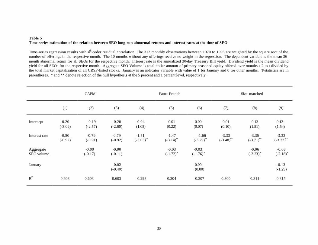
The time-series results are presented in Table 5. For all three abnormal return measures
and all specifications, the slope coefficient on interest rates is negative, implying that a one-
percentage point increase in annual interest rates is associated with SEO 3 year performance that
is roughly between 1% and 3% worse. These results are broadly consistent with the assertion that
these abnormal return measures proxy for mispricing and that the mispricing is related to holding
costs that are related to interest rates. This finding is strongly statistically significant for the
Fama-French three factor abnormal returns as well as the size-matched abnormal returns,
although the CAPM results are insignificant.
The coefficient on aggregate SEO volume as a fraction of total market capitalization is
negative for all specifications. This finding is statistically significant for both the Fama-French
three factor abnormal returns as well as the size-match abnormal returns. The CAPM results are
insignificant. For all specifications there is not a statistically significant difference between
offerings that occur in January versus other months.
8. Conclusions
Previous studies have debated whether poor post-SEO stock price performance violates
market efficiency. Inference is hampered by potential data-snooping biases and the fact that any
test of market efficiency is also a test of a specific model of market equilibrium. We provide a
methodology that avoids these problems.
This paper provides a different view of this post-SEO stock price performance by
acknowledging that mispricing provides profit opportunities for sophisticated investors. In the
absence of arbitrage costs, the trading activity of sophisticated investors will exert price impact
until all mispricing is eliminated. The existence of arbitrage costs implies that mispricing can
persist since not all corrective trades will be profitable. In equilibrium, securities with greater
arbitrage costs will exhibit greater potential mispricing.

18
We investigate three abnormal returns specifications based on the CAPM, the Fama-
French three factor model, and size matching. Overall, our results imply that the abnormal
returns estimated by these specifications are a manifestation of mispricing. Consistent with
costly arbitrage, abnormal returns are more negative during times of greater holding costs and for
stock which are subject to higher holding costs. Specifically, we find that abnormal performance
is related to interest rates, idiosyncratic risk, and dividend yields.
Interestingly, we do not find evidence that transaction costs are related to the abnormal
returns estimated by these specifications. Although previous studies have found relations
between abnormal returns and transaction cost proxies such as size, we show that once holding
costs are considered, a size relation is dwarfed. We posit that, for long-run mispricing, holding
costs are the predominant source of arbitrage costs rather than transaction costs.
19
References
Alexander, Gordon J., 2000, On back-testing "zero- investment" strategies, The Journal of Business 73, 255-278. Amihud, Y., and H. Mendelson, 1986, Asset pricing and the bid-ask spread, Journal of Financial Economics 17, 221-249. Banz, R. W., 1981, The relationship between return and market value of common stocks, Journal of Financ ial Economics 9, 3-18. Barber, Brad, and Lyon, J., 1997, Detecting long-run abnormal stock returns: The empirical power and specification of test statistics, Journal of Financial Economics 43, 341-372. Barber, Brad, Reuven Lehavy, Maureen McNichols, and Brett Trueman, 2000, Can investors profit from the prophets? Security analyst recommendations and stock returns, The Journal of Finance 56, 531-563. Bhardwaj, Ravinder K., and LeRoy D. Brooks, 1992, The January anomaly: effects of low share price, transaction costs, and bid-ask bias, The Journal of Finance 47, 553-575. Brav, Alon, 2000, Inference in long-horizon event studies: A Bayesian approach with application to initial public offerings, The Journal of Finance 55, 1979-2018. Brav, Alon, and Paul Gompers, 1997, Myth or reality? The long-run underperformance of initial public offerings: Evidence from venture and non-venture capital-backed companies, The Journal of Finance 52, 1791-1821. Brav, A., Geczy, C., and Gompers, P., 2000, Is the abnormal return following equity issuances anomalous?, Journal of Financial Economics 56, 209-249. Brennan, M. J., and A. Subrahmanyam, 1996, Market microstructure and asset pricing: On the compensation for illiquidity in stock returns, Journal of Financial Economics 41, 441-464. Chan, Louis K. C., and Josef Lakonishok, 1997, Institutional equity trading costs: NYSE versus Nasdaq, Journal of Finance 52, 713-735. Choi, James J., 2000, The Value Line enigma: The sum of known parts?, The Journal of Financial and Quantitative Analysis 35, 485-498. Copeland, Thomas E., and David Mayers, 1982, The Value Line Enigma (1965-1978) A case study of performance evaluation issues, Journal of Financial Economics 10, 289-321.

20
Dann, Larry Y., David Mayers, and Robert J. Raab, Jr., 1977, Trading rules, large blocks and the Speed of Price Adjustment, Journal of Financial Economics 4, 3-22. DeLong, J. Bradford, Andrei Shleifer, Lawrence H. Summers, and Robert J. Waldmann, 1990, Noise trader risk in financial markets, Journal of Political Economy 98, 703-738. Diamond, Douglas W., and Robert E. Verrecchia, 1987, Constraints on short-selling and asset price adjustment to private information, Journal of Financial Economics 18, 277-311. Eckbo, B. Espen, Ronald W. Masulis, and Oyvind Norli, 2000, Seasoned public offerings: resolution of the 'new issues puzzle', Journal of Financial Economics 56, 251-291. Fama, E. F, and M. Blume, 1966, Filter rules and stock market trading, Journal of Business 39, January, 226-241. Fama, Eugene, 1976, Foundations of Finance: Portfolio Decisions and Security prices, New York: Basic Books. Fama, Eugene, 1998, Market efficiency, long-term returns, and behavioral finance, Journal of Financial Economics 49, 283-306. Fama, Eugene, and Kenneth French, 1997, Industry costs of equity, Journal of Financial Economics 43, 153-193. Fama, Eugene F. and James D. MacBeth, 1973, Risk, return, and equilibrium: Empirical tests, Journal of Political Economy 71, 607-636. Friedman, Milton, 1953, The case for flexible exchange rates, in Essays in Positive Economics, Chicago, The University of Chicago Press. Garman, Mark B., and James A. Ohlson, 1981, Valuation of risky assets in arbitrage free economies with transaction costs, Journal of Financial Economics 9, 271-280. Jegadeesh, Narasimhan, 2000, Long-run performance of seasoned equity offerings: benchmark errors and biases in expectations, Financial Management 29, 5-30. Jensen, Michael C, and George A. Benington, 1970, Random walks and technical theories: Some additional evidence, The Journal of Finance, 469-482. Jones, Charles M., and Paul J. Seguin, 1997, Transaction costs and price volatility: Evidence from commission deregulation, American Economic Review 87, 729-737. Karpoff, Jonathan, and Ralph A. Walking, 1988, Short-term trading around ex-dividend days: Additional evidence, Journal of Financial Economics 21, 291-298.
21
Karpoff, Jonathan and Ralph A. Walkling, 1990, Dividend capture in Nasdaq stocks, Journal of Financial Economics 28, 39-65. Keim, Donald B. and Ananth Madhavan, 1998, The cost of institutional equity trades, Financial Analysts Journal, July/August, 50-69. Keim, Donald B., 1983, Size-related anomalies and stock return seasonality; further empirical evidence, Journal of Financial Economics 12, 13-32. Keynes, John M., 1936, The General Theory of Employment, Interest and Money, New York, Harcourt Brace. Knez, Peter J., and Mark J. Ready, 1996, Estimating the profits from trading strategies, The Review of Financial Studies 9, 1121-1163. Kothare, Meeta, and Paul A. Laux, 1995, Trading costs and the trading systems for Nasdaq stocks, Financial Analysts Journal, March-April, 42-53. Kothari, S., and Warner, J., 1997, Measuring long-horizon security price performance, Journal of Financial Economics 43, 301-309. Lesmond, David A., 2000, Post-earnings drift: A transaction costs perspective, Working paper, Tulane University. Lesmond, David, Joseph P. Ogden, and Charles A. Trzcinka, 1999, A new estimate of transaction costs, The Review of Financial Studies 12, 1113-1141. Lesmond, David, Michael J. Schill, and Chunsheng Zhou, 2001, The illusory nature of momentum profits, Working paper Tulane university and the University of California, Riverside. Litzenberger, R. and K. Ramaswamy, 1979, Dividends, short-selling restrictions, tax-induced investor clienteles and market equilibrium, Journal of Financial Economics 7, 163-196. Loughran, T., Ritter, J., 1995, The new issues puzzle, Journal of Finance 50, 23-51. Loughran, T., Ritter, J., 2000, Uniformly least powerful tests of market efficiency, Journal of Financial Economics, 55, 361-389. Malkiel, Burton G. and Yexiao Xu, 1997, Risk and returns revisited, The Journal of Portfolio Management, Spring, 9-14. Mech, Timothy, 1993, Portfolio return autocorrelation, Journal of Financial Economics 34, 307-344.
22
Mitchell, M., Stafford, E., 1998, Managerial decisions and long-term stock price performance, Journal of Business 73, 287-329. Myers, Stewart C., and Nicholas S. Majluf, 1984, Corporate financing and investment decisions when firms have information that investors do not have, Journal of Financial Economics 13, 187-221. Pontiff, Jeffrey, 1995, Closed-End Fund Premia and Returns: Implications for Financial Market Equilibrium, Journal of Financial Economics, 37. Pontiff, Jeffrey, 1996, Costly arbitrage: Evidence from closed-end funds, The Quarterly Journal of Economics 111, 1135-1151. Reinganum, M. R., 1981, Misspecification of capital asset pricing: Empirical anomalies based on earnings yields and market values, Journal of Financial Economics 9, 19-46. Ritter, Jay R., 1991, The long-run performance of initial public offerings, The Journal of Finance 46, 3-27. Rosett, R., 1959, A statistical model of friction in economics, Econometrica 27, 263-267. Schill, Michael, 2000, Market gaming? An examination of aggregate equity issue clustering, Working paper, UC Riverside. Shleifer, Andrei, and Robert W. Vishny, 1990, Equilibrium short horizons of investor and firms, American Economic Review 80, 148-153. Shleifer, Andrei, and Robert W. Vishny, 1997, The limits of arbitrage, The Journal of Finance 52, 35-56. Speiss, D. K., and J. Affleck-Graves, 1995, Underperformance in long-run stock returns following seasoned equity offerings, Journal of Financial Economics 38, 243-267. Stoll, H. R., and R. Whaley, 1983, Transactions costs and the small firm effect, The Journal of Financial Economics 12, 52-79. Tobin, J., 1958, Estimation of relationships for limited dependent variables, Econometrica 26, 24-36. Tuckman, Bruce, and Jean-Luc Vila, 1992, Arbitrage with holding costs: a utility based approach, The Journal of Finance 47, 1283-1302.
23
Table 1 Summary statistics The sample is comprised of all primary U.S. common seasoned equity offerings between January 1970 and December 1995 reported by SDC. Offerings by regulated utilities, REITs, and closed-end funds are excluded. Offerings which are not followed by CRSP are also excluded. Abnormal returns are estimated over 36 months beginning with the calendar month following the offering. Abnormal return specification is defined for model 1 using the estimated CAPM beta for offerings with at least six months of post-offering return data on CRSP otherwise the beta is set to one; for model 2 using the estimated Fama -French three-factor model loadings for offerings with more than 12 months of post-offering return data otherwise the model 1 estimate is used; for model 3 as the difference between buy-and-hold returns for the offering firm and that of a size-matched control firm. Idiosyncratic and beta risk are defined as the root mean square error and slope estimate from a regression of firm returns on the S&P 500 index over the three years prior to the offering. For firms with less than 12 return observations, the respective average industry root mean square error or beta estimate is used. Log of size is the natural logarithm of the market capitalization of the offering firm at the end of the calendar month of the offering. LDV is the limited dependent variable estimate of transaction costs. Inverse of price is the inverse of the offering firm's stock price at the end of the calendar month of the offering. Dividend yield is the past 12-month rolling dividend yield. Panel A: Sample statistics
Number
Mean
Std Dev
Minimum
Maximum
Abnormal return specification
(1) CAPM
5,302 -0.24 0.85 -4.06 5.09
(2) Fama-French
5,302 -0.14 0.91 -5.66 7.29
(3) Size-matched
5,284 -0.21 1.54 -16.09 17.87
Cross-sectional arbitrage cost variables
Idiosyncratic risk
5,302 0.14 0.07 0.03 0.78
Beta risk
5,302 1.31 0.77 -0.73 12.34
Log of size
5,302 -1.10 1.57 -6.51 4.82
LDV
5,302 0.06 0.06 -0.01 1.02
Inverse of price
5,302 0.11 0.47 0.00 21.33
Dividend yield
5,302 0.01 0.02 0.00 0.18
24
Table 1 (Continued) Summary statistics
Panel B: Abnormal return measure and cross-sectional variable correlation coefficients
Abnormal return specification
CAPM
Fama-French
Size-
matched
Idio. risk
Beta risk
Log of
size
LDV
Inverse of price
Abnormal return specification
Fama-French
0.875
Size-matched
0.548 0.498
Idiosyncratic risk
-0.130 -0.096 -0.063
Beta risk
-0.076 -0.041 -0.050 0.173
Log of size
0.039 0.048 0.011 -0.451 0.030
LDV
-0.018 -0.045 0.000 0.484 -0.037 -0.597
Inverse of price
0.017 0.001 0.011 0.199 -0.024 -0.244 0.373
Dividend yield
0.159 0.068 0.045 -0.442 -0.188 0.381 -0.265 -0.073
25
Table 2 Regression estimation of the relation between post-SEO long-run abnormal return measures and arbi trage cost proxies. Weighted least squares regression results. The sample is comprised of all primary U.S. common seasoned equity offerings between January 1970 and December 1995 reported by SDC. Offerings by regulated utilities, REITs, and closed-end funds are excluded. Offerings which are not followed by CRSP prior to the offering are also excluded. Variable descriptions are provided in Table 1. T-statistics are in parentheses. * and ** denote rejection of the null hypothesis at the 5 percent and 1 percent level, respectively. Regressions in Panel A and B contain 5303 observations. Regressions in panel C contain 5285 observations.
Panel A:
Dependent Variable:
CAPM 3 year Abnormal Return
(1)
(2)
(3)
(4)
(5)
(6)
(7)
(8)
Intercept
-0.18
(-3.50)
-0.34 (-7.04)
-0.23 (-4.64)
-0.19 (-3.61)
-0.18 (-3.55)
-0.05 (-0.92)
-0.40 (-9.77)
-0.18 (-3.48)
Idiosyncratic risk
-1.66 (-7.21)**
-1.77 (-7.79)**
-1.64 (-7.13)**
-1.67 (-7.67)**
-2.24 (-10.2)**
-1.58 (-7.59)**
Beta risk -0.05 (-2.75)**
-0.07 (-4.03)**
-0.05 (-2.88)**
-0.05 (-2.75)**
-0.07 (-4.54)**
-0.05 (-3.02) **
Log of size -0.02 (-1.63)
-0.01 (1.22)
-0.02 (-1.83)
-0.02 (-1.93)
0.00 (0.14)
0.04 (5.12)**
LDV -0.07 (-0.15)
-1.13 (-2.60) **
-0.04 (-0.08)
0.38 (1.05)
0.13 (0.28)
Dividend yield
5.54 (7.94)**
7.13 (10.73)**
5.95 (8.73)**
5.29 (7.77)**
5.53 (7.95)**
5.21 (7.70)**
Inverse of price
0.05 (1.46)
Adj. R2 0.069 0.060 0.068 0.069 0.069 0.058 0.029 0.069
26
Table 2 (Continued) Regression estimation of the relation between post-SEO long-run abnormal return measures and arbitrage cost proxies.
Panel B:
Dependent Variable:
Fama-French 3 Factor, 3 Year Abnormal Return
(1)
(2)
(3)
(4)
(5)
(6)
(7)
(8)
Intercept
0.17
(3.55)
0.06 (1.36)
0.13 (2.86)
0.16 (3.39)
0.17 (3.48)
0.20 (4.32)
-0.04 (-1.05)
0.16 (3.41)
Idiosyncratic risk
-1.38 (-5.90)**
-1.53 (-6.76)**
-1.33 (-5.74)**
-1.45 (-6.70)**
-1.49 (-6.65)**
-1.34 (-6.73)**
Beta risk -0.05 (-2.70)**
-0.07 (-4.26)**
-0.05 (-2.82)**
-0.04 (-2.65)**
-0.05 (-3.04)**
-0.05 (-2.83)**
Log of size -0.01 (-1.63)
-0.01 (-0.95)
-0.02 (-1.83)
-0.01 (-1.41)
-0.01 (-1.24)
0.02 (2.93)**
LDV -0.33 (-0.84)
-1.24 (-3.28)**
-0.26 (-0.65)
0.04 (0.11)
-0.20 (-0.49)
Dividend yield
0.66 (1.73) *
1.30 (3.52)**
0.84 (2.22)*
0.51 (1.37)
0.60 (1.60)
0.50 (1.36)
Inverse of price
0.02 (0.54)
Adj. R2 0.016 0.009 0.015 0.015 0.016 0.015 0.001 0.015
27
Table 2 (Continued) Regression estimation of the relation between post-SEO long-run abnormal return measures and arbitrage cost proxies.
Panel C:
Dependent Variable:
Size-matched, 3 Year Abnormal Return
(1)
(2)
(3)
(4)
(5)
(6)
(7)
(8)
Intercept
0.03 (0.36)
-0.12 (-1.48)
-0.02 (-0.26)
0.03 (0.35)
0.04 (0.43)
0.07 (0.79)
-0.19 (-2.71)
0.04 (0.45)
Idiosyncratic risk
-1.53 (-3.83)**
-1.66 (-4.23)**
-1.51 (-3.87)**
-1.38 (-3.62)**
-1.68 (-4.39)**
-1.41 (-3.94) **
Beta risk -0.05 (-1.85)*
-0.07 (-2.59)**
-0.05 (-1.87)*
-0.06 (-1.96)*
-0.06 (-2.14)*
-0.05 (-1.95) *
Log of size -0.00 (-0.17)
0.01 (0.60)
-0.00 (-0.31)
-0.01 (-0.79)
0.00 (0.16)
0.02 (1.90) *
LDV 0.60 (1.24)
0.06 (0.12)
0.67 (1.40)
0.63 (1.46)
0.64 (1.34)
Dividend yield
1.48 (1.26)
2.80 (2.49)**
1.90 (1.65) *
1.43 (1.26)
1.59 (1.36)
1.35 (1.18)
Inverse of price
0.13 (2.29)
Adj. R2 0.008 0.006 0.008 0.009 0.008 0.008 0.003 0.009
28
Table 3 Regression results varying the time horizon of the dependent variable Weighted least squares regression results. The sample is comprised of all primary U.S. common seasoned equity offerings between January 1970 and December 1995 reported by SDC. Offerings by regulated utilities, REITs, and closed-end funds are excluded. Offerings which are not followed by CRSP prior to the offering are also excluded. Variable descriptions are provided in Table 1. Abnormal returns measured from first calendar month following the offering to 24 or 48 months following the offering. T-statistics are in parentheses. * and ** denote rejection of the null hypothesis at the 5 percent and 1 percent level, respectively.
Dependent variable
CAPM
Fama-French
Size-matched
2 years
4 years
2 years
4 years
2 years
4 years
Intercept
-0.13
(-3.24)
-0.20
(-2.15)
0.06
(1.59)
0.20
(2.49)
-0.00
(-0.05)
0.31
(2.13) *
Idiosyncratic risk -1.29 (-7.09)**
-1.67 (-6.19)**
-0.87 (-4.59)**
-1.51 (-5.54)**
-1.53 (-3.80)**
-1.50 (-3.61)**
Beta risk -0.03 (-2.59)**
-0.07 (-3.67)**
-0.02 (-1.84)*
-0.09 (-4.27)**
-0.05 (-1.71) *
-0.06 (-2.15)*
Log of size -0.02 (-2.13)
-0.01 (-0.55)
-0.02 (-2.37)
-0.01 (-0.84)
-0.01 (-0.42)
0.00 (0.24)
LDV -0.29 (-0.77)
0.27 (0.50)
-0.73 (-2.09) *
-0.30 (-0.75)
-0.47 (-0.96)
0.65 (1.25)
Dividend yield
3.85 (7.07) **
6.34 (7.60)**
0.75 (2.09) *
0.14 (0.29)
1.56 (1.33)
1.64 (1.37)
Observations
5666 4870 5666 4870 5284 4852
Adj. R2 0.061 0.066 0.012 0.019 0.009 0.011
29
Table 4 Fama-MacBeth estimation of the universal relation between arbitrage costs and abnormal returns The sample is comprised of all securities covered by CRSP with December year-end data from 1969 to 1995. Variable descriptions are provided in Table 1. For each of the 26 years, a cross-sectional regression is estimated of three-year abnormal return measures on arbitrage costs proxies. The reported slope-coefficients are the average slope coefficient from each regression. T-statistics are in parentheses. The standard errors are adjusted for second-order serial dependence. * and ** denote rejection of the null hypothesis at the 5 percent and 1 percent level, respectively.
Dependent Variable
CAPM
3 year Abnormal Return
Fama-French 3 Factor
3 Year Abnormal Return
(1)
(2)
(3)
(4)
(5)
(6)
Intercept
0.26
(3.12)**
0.04
(2.34) *
0.32
(3.10) **
0.17
(2.98) **
0.04 (2.57) *
0.11
(0.87)
Idiosyncratic risk
-0.25 (-1.30)
0.08 (0.36)
-0.01 (-0.05)
-0.17 (-0.87)
-0.12 (-0.66)
0.00 (0.01)
Beta risk -0.03 (-1.69)
-0.04 (-2.17) *
-0.03 (-1.81)
-0.03 (-1.15)
Log of size -0.01 (-1.88)
-0.02 (-2.30) *
-0.01 (-2.08) *
-0.00 (-0.24)
Dividend yield
0.31 (0.96)
0.61 (1.85)
0.30 (0.93)
-0.59 (-2.66) *
-0.40 (-2.15) *
-0.57 (-1.74)
Inverse of price
0.14 (0.33)
0.08 (1.79)
30
Table 5 Time-series estimation of the relation between SEO long-run abnormal returns and interest rates at the time of SEO Time -series regression results with 4th-order residual correlation. The 312 monthly observations between 1970 to 1995 are weighted by the square root of the number of offerings in the respective month. The 10 months without any offerings receive no weight in the regression. The dependent variable is the mean 36-month abnormal return for all SEOs for the respective month. Interest rate is the annualized 30-day Treasury Bill yield. Dividend yield is the mean dividend yield for all SEOs for the respective month. Aggregate SEO Volume is total dollar amount of primary seasoned equity offered over months t-2 to t divided by the total market capitalization of all CRSP-listed stocks. January is an indicator variable with value of 1 for January and 0 for other months. T-statistics are in parentheses. * and ** denote rejection of the null hypothesis at the 5 percent and 1 percent level, respectively.
CAPM
Fama-French
Size-matched
(1)
(2)
(3)
(4)
(5)
(6)
(7)
(8)
(9)
Intercept
-0.20
(-3.09)
-0.19
(-2.57)
-0.20
(-2.60)
-0.04 (1.05)
0.01
(0.22)
0.00
(0.07)
0.01
(0.10)
0.13
(1.51)
0.13
(1.54)
Interest rate -0.80 (-0.92)
-0.79 (-0.91)
-0.79 (-0.92)
-1.51 (-3.03)**
-1.47 (-3.14)**
-1.66 (-3.29)**
-3.33 (-3.48)**
-3.35 (-3.71)**
-3.33 (-3.72)**
Aggregate SEO volume
-0.00
(-0.17) -0.00
(-0.11) -0.03
(-1.72) * -0.03
(-1.76) * -0.06
(-2.23) * -0.06
(-2.18) *
January
-0.02
(-0.40) 0.00
(0.00) -0.13
(-1.29)
R2 0.603 0.603 0.603 0.298 0.304 0.307 0.300 0.311 0.315