Long-term changes in theLong-term changes in thegeomagnetic fieldgeomagnetic field

Monika Korte,Monika Korte,GeoForschungsZentrumGeoForschungsZentrum Potsdam Potsdam

Acknowledgements:Acknowledgements:Development and study of the Development and study of the CALSxKCALSxK models are a close models are a closecollaboration with Catherine Constable.collaboration with Catherine Constable.

We owe special thanks to We owe special thanks to AgnAgnèsès GeneveyGenevey, who compiled and, who compiled andcarefully checked a large global carefully checked a large global archeointensityarcheointensity dataset. dataset.

The new global descriptions of the past geomagnetic field would notThe new global descriptions of the past geomagnetic field would nothave been possible without the work of many colleagues, who carriedhave been possible without the work of many colleagues, who carriedout the tedious task of collecting and measuring out the tedious task of collecting and measuring archeoarcheo- and- andpaleomagneticpaleomagnetic data from around the world. data from around the world.

OutlineOutline

Archeomagnetic data and their uncertainties

Commonly used methods:Paleo-secular variationVDMs and VADMs

Global spherical harmonic modelsMethodResolution and reliability

A new dipole moment estimate

Regional secular variation differences

Summary

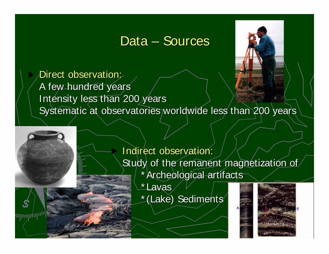
Data Data –– Sources Sources

Direct observation:Direct observation:A few hundred yearsA few hundred yearsIntensity less than 200 yearsIntensity less than 200 yearsSystematic at observatories worldwide less than 200 yearsSystematic at observatories worldwide less than 200 years

Indirect observation:Indirect observation:Study of the Study of the remanentremanent magnetization of magnetization of

*Archeological artifacts*Archeological artifacts*Lavas*Lavas*(Lake) Sediments*(Lake) Sediments

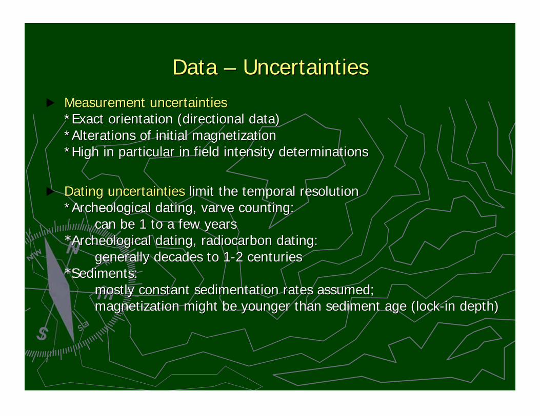
Data Data –– Uncertainties Uncertainties

Measurement uncertaintiesMeasurement uncertainties*Exact orientation (directional data)*Exact orientation (directional data)*Alterations of initial magnetization*Alterations of initial magnetization*High in particular in field intensity determinations*High in particular in field intensity determinations

Dating uncertaintiesDating uncertainties limit the temporal resolution limit the temporal resolution*Archeological dating, *Archeological dating, varvevarve counting: counting:

can be 1 to a few yearscan be 1 to a few years*Archeological dating, radiocarbon dating:*Archeological dating, radiocarbon dating:

generally decades to 1-2 centuriesgenerally decades to 1-2 centuries*Sediments:*Sediments:

mostly constant sedimentation rates assumed;mostly constant sedimentation rates assumed;magnetization might be younger than sediment age (lock-in depth)magnetization might be younger than sediment age (lock-in depth)

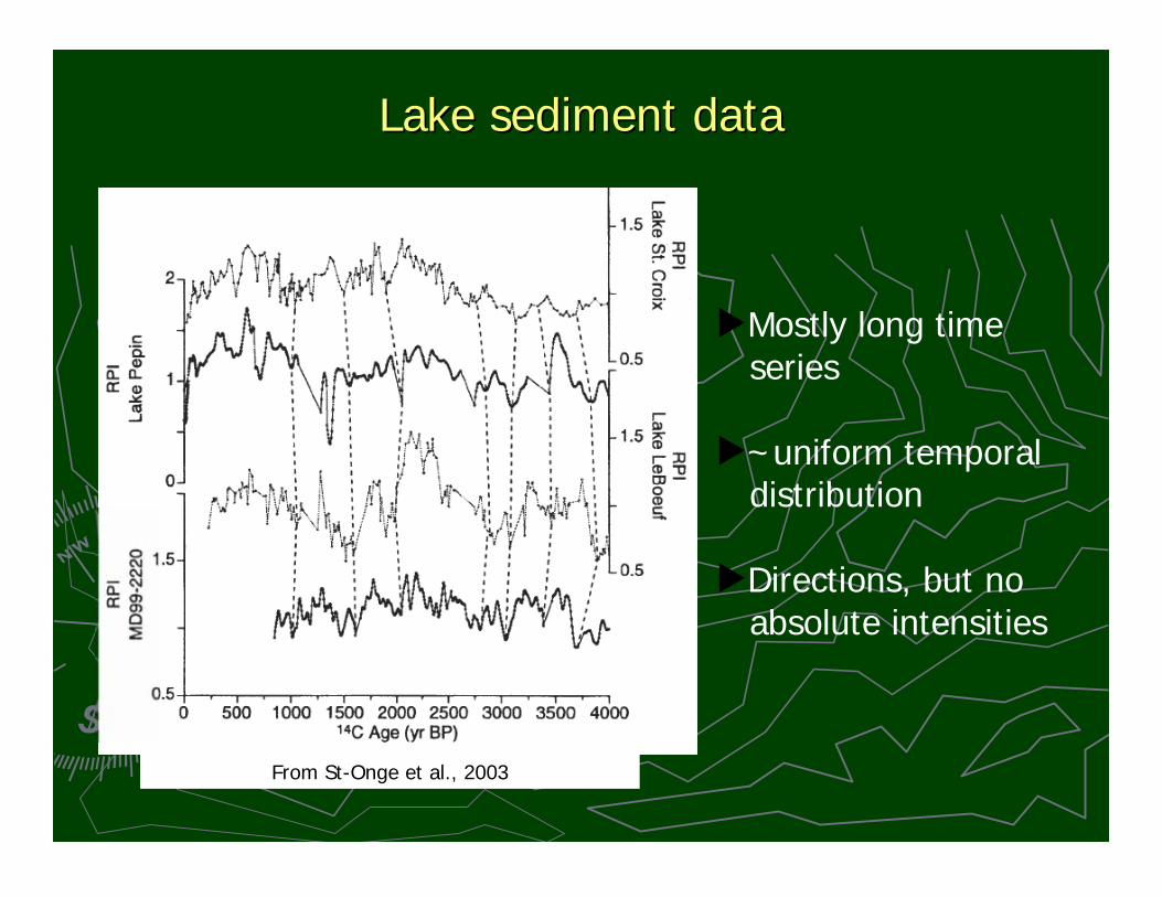
Lake sediment dataLake sediment data

Mostly long time series

~uniform temporal distribution

Directions, but no absolute intensities

From St-Onge et al., 2003

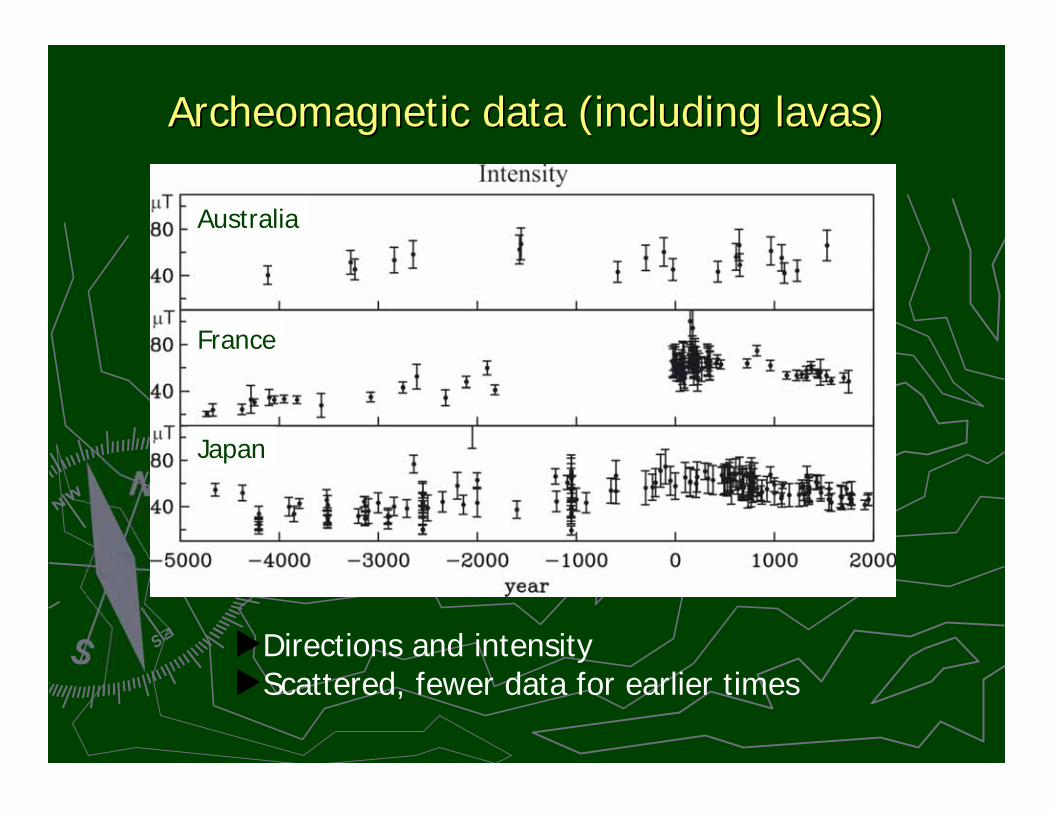
ArcheomagneticArcheomagnetic data (including lavas) data (including lavas)

Directions and intensityScattered, fewer data for earlier times

Australia

France

Japan

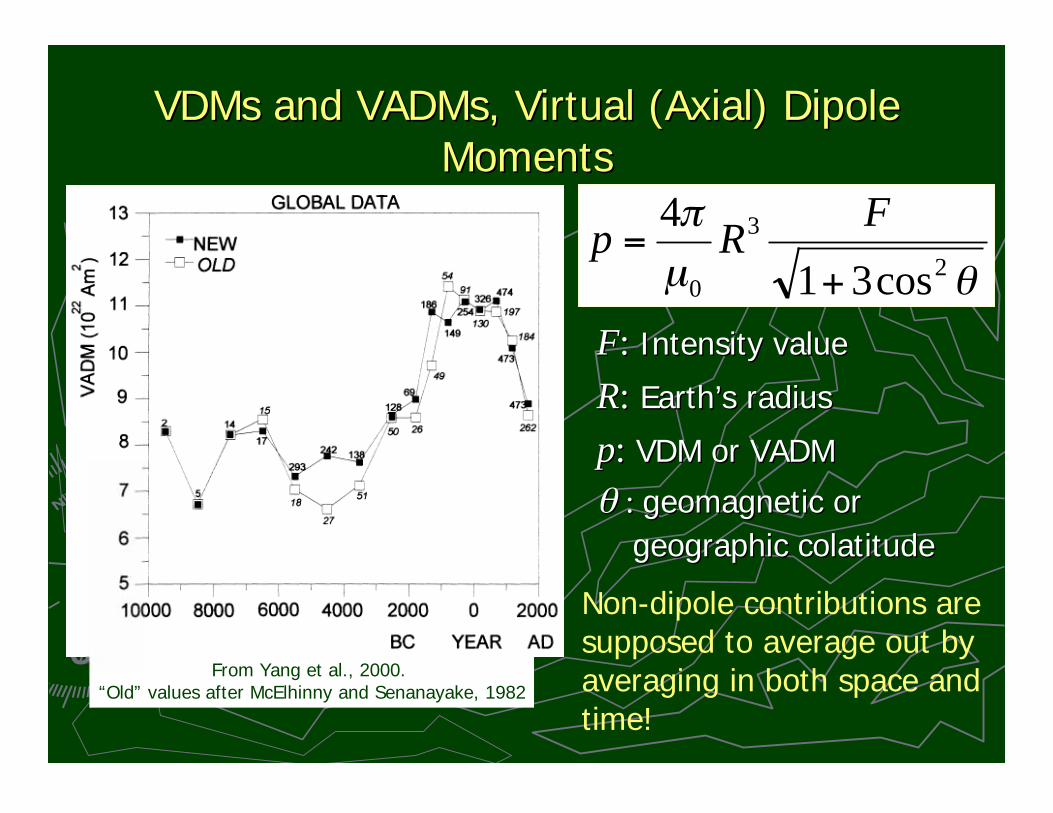
VDMsVDMs and and VADMsVADMs, Virtual (Axial) Dipole, Virtual (Axial) DipoleMomentsMoments

FF:: Intensity value Intensity value

RR:: Earth Earth’’s radiuss radius

pp:: VDM or VADM VDM or VADM

: : geomagnetic orgeomagnetic or

geographic geographic colatitudecolatitude

μ 2

3

0 cos31

4

+=

FRp

From Yang et al., 2000. “Old” values after McElhinny and Senanayake, 1982

Non-dipole contributions aresupposed to average out byaveraging in both space andtime!

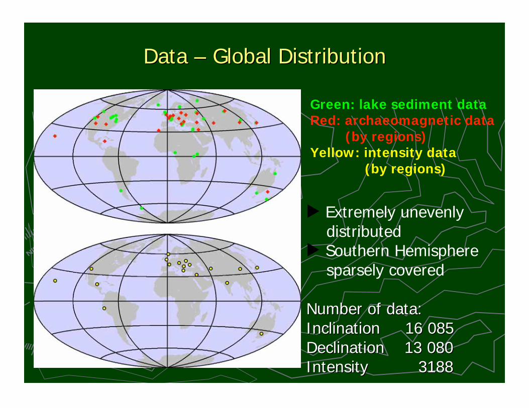
Data Data –– Global Distribution Global Distribution

Green: lake sediment dataRed: archaeomagnetic data

(by regions)Yellow: intensity data

(by regions)

Extremely unevenly distributed

Southern Hemisphere sparsely covered

Number of data:Number of data:Inclination 16 085Inclination 16 085Declination 13 080Declination 13 080Intensity 3188Intensity 3188

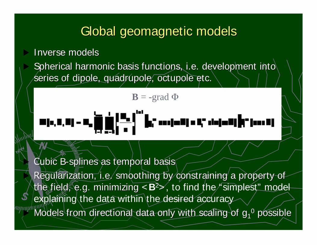
Global geomagnetic modelsGlobal geomagnetic models

Inverse modelsInverse models

Spherical harmonic basis functions, i.e. development intoSpherical harmonic basis functions, i.e. development intoseries of dipole, series of dipole, quadrupolequadrupole, , octupoleoctupole etc. etc.

Cubic B-Cubic B-splinessplines as temporal basis as temporal basis

Regularization, i.e. smoothing by constraining a property ofRegularization, i.e. smoothing by constraining a property ofthe field, e.g. minimizing the field, e.g. minimizing <B2>, to find the “simplest” modelexplaining the data within the desired accuracy

Models from directional data only with scaling of gModels from directional data only with scaling of g1100 possible possible

B = -grad

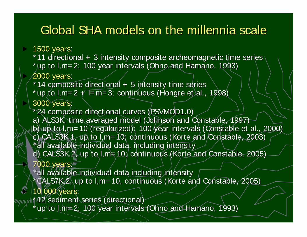
Global SHA models on the millennia scaleGlobal SHA models on the millennia scale

1500 years1500 years::*11 directional + 3 intensity composite *11 directional + 3 intensity composite archeomagneticarcheomagnetic time series time series*up to *up to l,ml,m=2; 100 year intervals (=2; 100 year intervals (OhnoOhno and Hamano, 1993) and Hamano, 1993)

2000 years2000 years::*14 composite directional + 5 intensity time series*14 composite directional + 5 intensity time series*up to *up to l,ml,m=2 + l=m=3; continuous (=2 + l=m=3; continuous (HongreHongre et al., 1998) et al., 1998)

3000 years3000 years::*24 composite directional curves (PSVMOD1.0)*24 composite directional curves (PSVMOD1.0)a) ALS3K, time averaged model (Johnson and Constable, 1997)a) ALS3K, time averaged model (Johnson and Constable, 1997)b) up to b) up to l,ml,m=10 (regularized); 100 year intervals (Constable et al., 2000)=10 (regularized); 100 year intervals (Constable et al., 2000)c) CALS3K.1, up to c) CALS3K.1, up to l,ml,m=10; continuous (Korte and Constable, 2003)=10; continuous (Korte and Constable, 2003)*all available individual data, including intensity*all available individual data, including intensityd) CALS3K.2, up to d) CALS3K.2, up to l,ml,m=10; continuous (Korte and Constable, 2005)=10; continuous (Korte and Constable, 2005)

7000 years7000 years::*all available individual data including intensity*all available individual data including intensity*CALS7K.2, up to *CALS7K.2, up to l,ml,m=10, continuous (Korte and Constable, 2005)=10, continuous (Korte and Constable, 2005)

10 000 years10 000 years::*12 sediment series (directional)*12 sediment series (directional)*up to *up to l,ml,m=2; 100 year intervals (=2; 100 year intervals (OhnoOhno and Hamano, 1993) and Hamano, 1993)

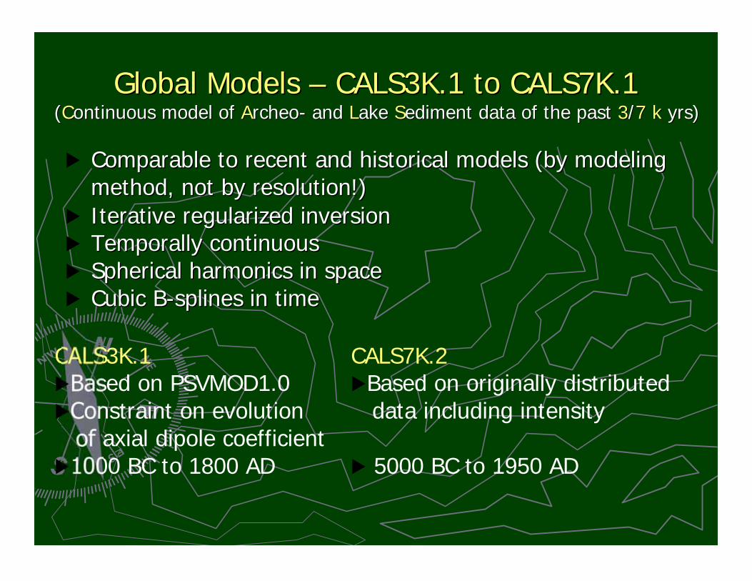
Global Models Global Models –– CALS3K.1 to CALS7K.1 CALS3K.1 to CALS7K.1((CContinuous model of ontinuous model of AArcheorcheo- and - and LLake ake SSediment data of the past ediment data of the past 33//77 kk yrs) yrs)

Comparable to recent and historical models (by modelingComparable to recent and historical models (by modelingmethod, not by resolution!)method, not by resolution!)

Iterative regularized inversionIterative regularized inversionTemporally continuousTemporally continuousSpherical harmonics in spaceSpherical harmonics in spaceCubic B-Cubic B-splinessplines in time in time

CALS3K.1Based on PSVMOD1.0Constraint on evolution

of axial dipole coefficient1000 BC to 1800 AD

CALS7K.2Based on originally distributed

data including intensity

5000 BC to 1950 AD

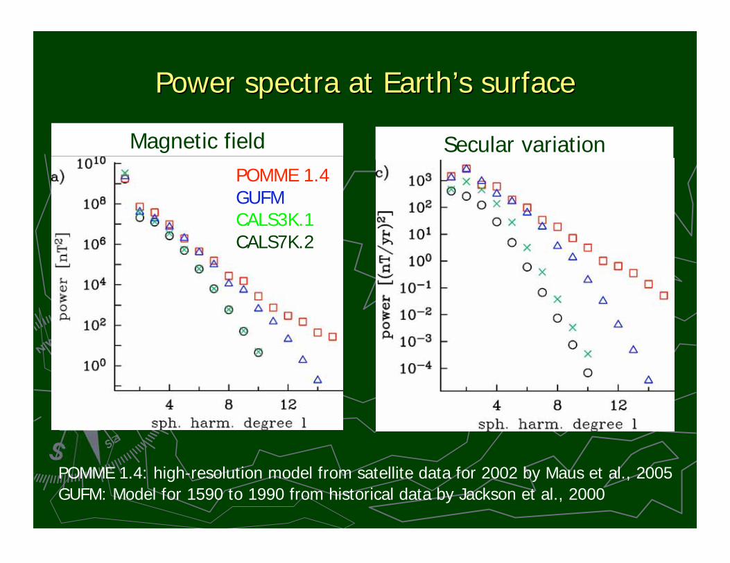
Power spectra at EarthPower spectra at Earth’’s surfaces surface

Magnetic field Secular variation

POMME 1.4GUFMCALS3K.1CALS7K.2

POMME 1.4: high-resolution model from satellite data for 2002 by Maus et al., 2005 GUFM: Model for 1590 to 1990 from historical data by Jackson et al., 2000

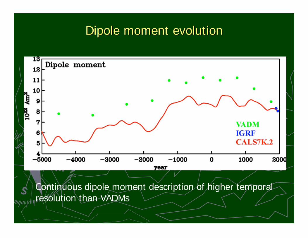
Dipole moment evolutionDipole moment evolution

Continuous dipole moment description of higher temporalresolution than VADMs

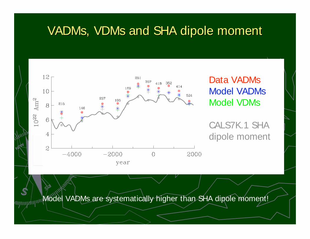
VADMsVADMs, , VDMsVDMs and SHA dipole moment and SHA dipole moment

Data VADMsModel VADMsModel VDMs

CALS7K.1 SHAdipole moment

Model VADMs are systematically higher than SHA dipole moment!

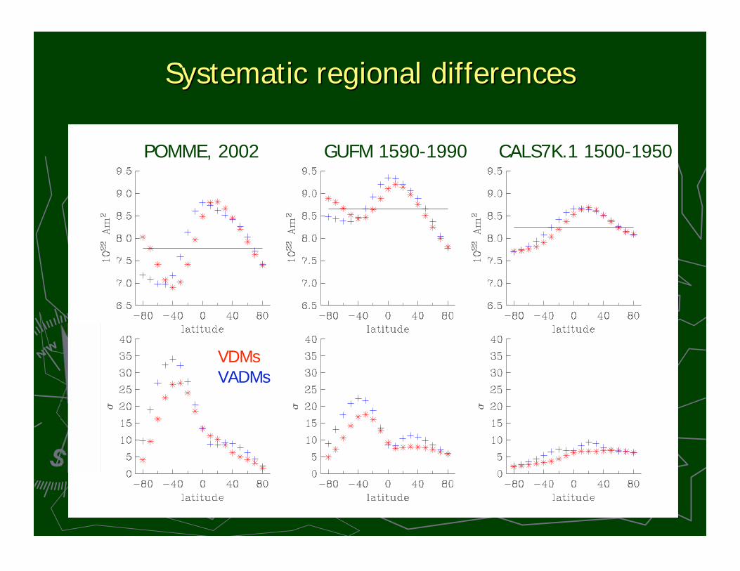
Systematic regional differencesSystematic regional differences

VDMsVADMs

POMME, 2002 GUFM 1590-1990 CALS7K.1 1500-1950

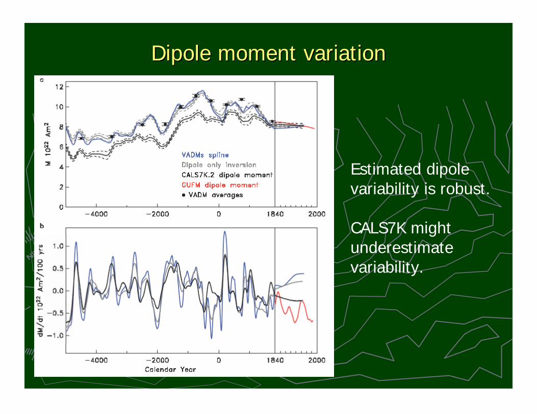
Dipole moment variationDipole moment variation

Estimated dipolevariability is robust.

CALS7K might underestimatevariability.

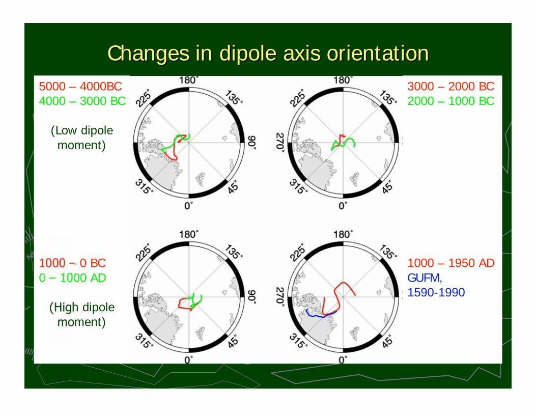
Changes in dipole axis orientationChanges in dipole axis orientation

5000 – 4000BC4000 – 3000 BC

(Low dipolemoment)

1000 – 0 BC0 – 1000 AD

(High dipolemoment)

3000 – 2000 BC2000 – 1000 BC

1000 – 1950 ADGUFM,1590-1990

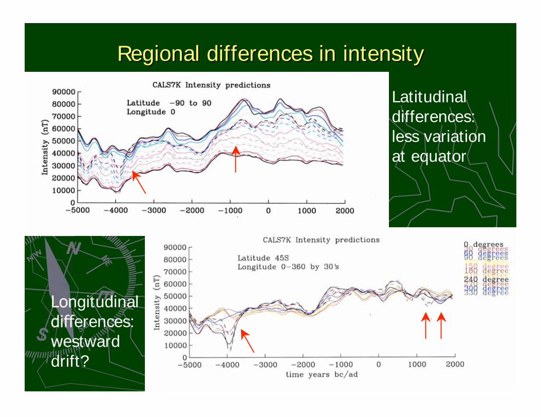
Regional differences in intensityRegional differences in intensity

Latitudinaldifferences:less variationat equator

Longitudinaldifferences:westwarddrift?

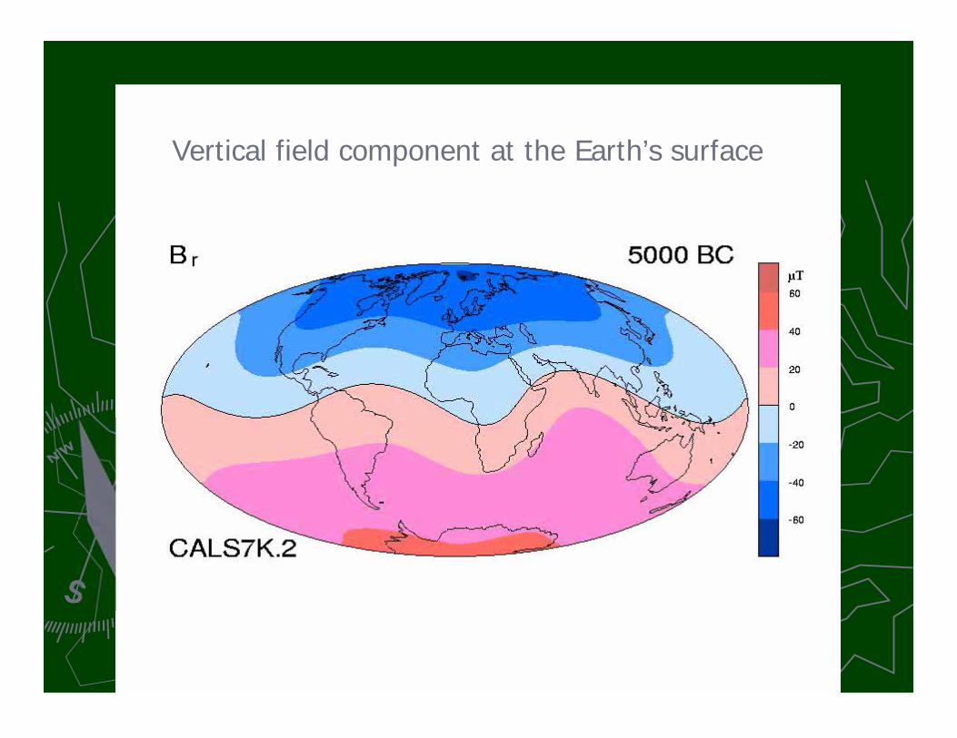
Vertical field component at the Earth’s surface

SummarySummary

Global magnetic field models on the millennia scale are a useful tool toGlobal magnetic field models on the millennia scale are a useful tool todescribe and study the evolution of the geomagnetic field.describe and study the evolution of the geomagnetic field.

We have to be careful about the robustness of models and be awareWe have to be careful about the robustness of models and be awareof their limitations which are imposed by the data. The large-scaleof their limitations which are imposed by the data. The large-scalefeatures, however, have proven quite robust.features, however, have proven quite robust.

The increasing amount of The increasing amount of paleomagneticpaleomagnetic data on the millennia scale data on the millennia scalewill improve global field models further in the future. An extension ofwill improve global field models further in the future. An extension ofcontinuous global models to 10 continuous global models to 10 kyrkyr seems feasible. seems feasible.

Global models suggest that the dipole moment of the past millenniaGlobal models suggest that the dipole moment of the past millenniahas been overestimated by previous VADM descriptions. Moreover,has been overestimated by previous VADM descriptions. Moreover,global models offer a significantly improved temporal resolution.global models offer a significantly improved temporal resolution.