Long-Term Government Debt and Household Portfolio

Composition

Andreas Tischbirek∗

University of Lausanne

This version: December 2018

Abstract

Formal dynamic analyses of household portfolio choice in the literature focus on

holdings of equity and a risk-free asset or bonds of different maturities, neglecting

the interdependence of the decisions to invest in equity, short-term and long-term

bonds made by households. Data from the Survey of Consumer Finances is used

to derive stylised facts about participation in the long-term government-debt mar-

ket and conditional portfolio shares. To explain the mechanisms underlying these

facts, I draw on a life-cycle model in which investors have access to three financial

assets—equity, long-term debt and a riskless short-term bond—and are exposed

to uninsurable idiosyncratic risk through non-financial income as well as aggregate

risk through the asset returns. An application shows that the low Treasury returns

observed in the US between 2009 and 2013 have quantitatively significant yet tran-

sitory effects on the composition of household portfolios. In combination with the

observed rise in stock returns, they lead to persistent changes in the participation

rate, the conditional portfolio shares and the distribution of wealth.

Keywords: Dynamic Portfolio Choice, Life Cycle, Long-Term Government Debt, Asset-

Market Participation, Survey of Consumer Finances

JEL-Classification: D10, D15, E21, G11∗Department of Economics, HEC Lausanne, University of Lausanne

E-mail: andreas.tischbirek@unil.chI would like to thank Guido Ascari, Wouter den Haan, Martin Ellison, Elisa Faraglia, Francisco Gomes,Charles Gottlieb, Winfried Koeniger, Pascal St-Amour as well as a number of seminar and conferenceparticipants for helpful comments and discussions. Financial support from the Royal Economic Societyis gratefully acknowledged.

1 Introduction

Analyses of portfolio choice over the life cycle generally focus on holdings of stock and a

risk-free asset, not taking into account the significant positions of long-term government

debt that can be found in household portfolios. With short-term nominal interest rates

close to the zero lower bound in Europe and the US in the aftermath of the the Financial

Crisis of 2007 to 2009, central banks have purchased large amounts of long-term debt as a

part of their unconventional monetary policy programmes. In this context, the role that

long-term bonds play in household portfolios and the motives for rebalancing portfolios

in response to return shocks have become of considerable interest. Using a life-cyle model

in which agents can invest in three financial assets—stocks, long-term government debt

and a riskless asset—this paper studies the decision to participate in financial markets

and the composition of household portfolios over the course of the life cycle with a focus

on the role of long-term government debt.

Stylised facts are derived based on a data set constructed from seven consecutive waves

of the Survey of Consumer Finances (SCF). The joint existence of birth cohort, time and

age influences on the participation rate and the respective portfolio shares conditional

on participation result in a well-known identification problem.1 Using three different

identification strategies, two from the literature and one novel, a latent variable model with

a participation equation is estimated. The standard approach based on cohort restrictions

performs the least well. The remaining two, although distinct, give nearly identical results.

Similar to participation in the stock market, participation in the market for long-term

debt takes an inverse U-shape. While the conditional portfolio share of stocks is declining

with age, the conditional share of long-term government debt is moderately increasing

until the age of around 55 and significantly lowered from about 65 onwards.2 Long-term

bond holdings and holdings of the riskless asset differ with respect to their elasticities

of substitution with equity, suggesting that the shares of long-term debt and the riskless

asset are rebalanced in distinctive ways in response to wealth and return shocks.

The theoretical analysis is based on a model in which agents adjust consumption and

holdings of the three financial assets facing uninsurable labour or retirement income risk as

well as random stock and long-term debt returns. Fixed participation costs prevent agents

from investing in stocks and government debt at young age. The participation rate first

rises as they accumulate wealth and later declines due to agents retiring and running down

1 Browning et al. (2012) give a detailed description of the “age-period-cohort” problem. According tothem, the problem can be traced back at least to Ryder (1965). See also Ameriks and Zeldes (2004).

2 The results regarding equity holdings are in line with findings by Fagereng et al. (2017) and Gomesand Michaelides (2005)

1

their savings. The average long-term debt and stock share conditional on participation

respectively increases and decreases with age during the employment stage in line with the

data. This is the case, since the portfolio income of market participants grows on average,

implying that the ratio of portfolio to labour income rises. As a result, agents with CRRA

utility rebalance their portfolios to reduce their risk exposure. Long-term debt plays an

important part in this process, because its return is less volatile than that of stocks but

higher in expectation than that of the risk-free asset. Incompleteness of financial markets

gives rise to a non-degenerate distribution of wealth. Agents that consistently participate

in the markets for equity and debt at a young age accumulate wealth faster than those that

enter later or remain stuck below the participation threshold, implying that the wealth

distribution among employed investors shows the characteristic positive skew found in the

data and that inequality increases with age.

Finally, the model is used to study the period of negative real 5-year Treasury returns

and elevated real stock returns that followed the recession of 2007 to 2009 in the US. In

the model, the Treasury return shocks observed between 2009 and 2013, when consid-

ered in isolation, lead to a significant rebalancing of household portfolios towards stock

holdings. The adjustments are transitory though during the employment stage. This is

the case, because the negative effect of the debt return shocks on the portfolio return are

compensated by the higher stock share so that wealth and hence the participation rate are

nearly unaffected. Consequently, the initial adjustments are undone when the Treasury

return rises again. The observed shocks to the returns of both assets jointly cause average

wealth to rise and the participation rate to increase. The change in average wealth has

persistent effects on the holdings of all three assets and the wealth distribution among

agents that are hit by the shocks at an intermediate age is more unequal for the remainder

of nearly their entire lives.

A large literature is concerned with portfolio choice over the life cycle. Early contri-

butions by Merton (1969, 1971) and Samuelson (1969) analyse optimal portfolio choice

neglecting the asset market participation decision. More recent examples include, but

are not limited to, Alan (2006), Bonaparte et al. (2012), Campanale et al. (2015), Cocco

et al. (2005), Fagereng et al. (2017), Gomes and Michaelides (2005) and Haliassos and

Michaelides (2003).3 In these papers, households are restricted to holdings of stocks and

a riskless asset. I relax this constraint by adding a long-term bond to the portfolio choice

problem. Bagliano et al. (2014) study a life-cycle model with a safe asset and two risky

assets focusing on how the portfolio shares evolve when the stock return is correlated

3 The model follows this literature in abstracting from informational frictions or incentive problemsthat may arise if households delegate the portfolio-choice decision to a portfolio manager.

2

with labour income. They assume that the second risky asset is identical to stocks aside

from the mean and variance of its return, not incorporating characteristics of long-term

bond returns like a realistic degree of autocorrelation. Campbell and Viceira (2001) and

Wachter (2003) consider asset allocation problems with long-term bonds but do not study

life-cycle effects. In the model used here, long-term debt is only partially liquid, reflecting

the fact that long-term debt like US savings bonds can be sold only at a substantial cost

in the first years after they have been issued. As in Campanale et al. (2015), the compo-

sition of financial wealth therefore becomes an important state variable in the portfolio

choice problem. While they assume that only holdings of the risk-free asset can be trans-

formed costlessly into consumption, the portfolio composition matters here because of a

maturity-specific liquidity constraint.

The paper is organised as follows. Section 2 presents the empirical results. It starts

by describing the data set, then gives a detailed discussion of the identification strategies

employed and finally shows the estimation results. Section 3 contains a description of the

model, its calibration and the resulting policy functions. In Section 4, model simulations

are confronted with the data and the model is applied to the 2009-2013 period in the US.

Section 5 concludes.

2 Stylised Facts

This section presents stylised facts on long-term government bond and stock holdings

of US households which inform and provide a benchmark for the model-based analysis

that follows. With the purely descriptive approach many times adopted in the literature,

adjustments of conditional asset shares cannot be reliably isolated from changes at the

extensive margin and life-cycle effects cannot be reliably isolated from sampling period

and cohort effects.4 The section therefore contains a careful discussion of the models

estimated and the strategies used to achieve parameter identification.

2.1 Data

The data set employed is constructed from the seven consecutive waves of the SCF col-

lected between 1989 and 2007.5 Since the data consist of repeated cross-sections rather

4 A notable exception is Fagereng et al. (2017) who equally account for the participation decision byestimating a latent variable model and use a set of strategies to address the age-period-cohort problemwhich partially overlaps with that employed here but focus solely on the stock market.

5 Data from later years are not used here to avoid bias introduced by crisis-specific effects. Data frombefore 1989 are not used due to changes in the availability of a subset of variables.

3

than a panel, I am not able to track individuals over time. However, due to the large

amount of households included in each survey wave, one can track cohorts of individuals

defined by their birth year over the sample period.6

It should be noted that there is an intentional oversampling of wealthy households in

the SCF relative to the US population. This is done to allow for more precise estimates

of financial asset holdings, which are highly concentrated among households in the upper

tail of the wealth distribution, and to correct for the fact that the non-response rate

is positively correlated with wealth (Kennickell, 2008). The benefit of much improved

estimation precision comes at the cost of being able to make inferences for wealthier

households only. Nonetheless, I believe that uncovering the life-cycle patterns in asset

holdings among those that are the likely holders of the assets in question is of considerable

interest. Descriptive statistics of the sample are shown in Table 1.

Variable Mean Variance Min Max

Household (h.h.) compositionAge of h.h. head 50.32 10.04 26 76Marital Status of h.h. head 0.74 0.44 0 1Number of children living in h.h. 0.98 1.20 0 10

Family income (gross, in thousands)Wages 210.04 1,143.30 -86.92 88,630.81Interest, dividends 112.17 981.75 0 51,550.12Sales of stocks, bonds, real estate 149.97 1,795.72 -1,759.41 114,890.5Retirement income, pensions, annuities 7.60 75.46 0 6,550.77Other, transfers 6.05 232.04 -1,450.44 57,408.45

Highest education of h.h. headNone 0.07 0.26 0 1School diploma 0.24 0.42 0 1Some college education 0.16 0.36 0 1College diploma 0.53 0.50 0 1

Ethnic background of h.h. headWhite and non-Hispanic 0.84 0.36 0 1Black 0.08 0.27 0 1Hispanic 0.04 0.20 0 1Other 0.04 0.19 0 1

Occupational category of h.h. headManagerial and professional 0.45 0.50 0 1Technical, sales and services 0.21 0.41 0 1Other 0.18 0.39 0 1Not working 0.15 0.36 0 1

Notes: Nominal variables in 2010 US dollars.

Table 1: Descriptive statistics

The SCF contains information on a large variety of assets held by households, which

I divide into three categories. These categories are long-term government debt, stocks

6 This fact was pointed out by Deaton and Paxson (1994) and Deaton (1997).

4

and a residual category that mainly includes cash/liquidity, short-term sovereign debt

and corporate bonds. Most assets that appear in household balance sheets can be fully

attributed to one of these three categories. When this is not the case, a careful partial

assignment is done based on additional information about the institutions that issue the

asset in question.

According to the “Monthly Statement of the Public Debt of the United States” from

December 2007, 22.1% of total marketable debt held by the public took the form of Bills

(maturity of one year or less), while the remaining 77.9% were issued in the form of Notes,

Bonds and TIPS (maturity of two years or more). Assuming that agents are homogeneous

in regards to the maturity composition of government debt in their portfolios, 77.9% of the

marketable US government debt held by a household is assigned to long-term government

debt and the remaining part to the residual category. Savings bonds and tax-exempt

bonds, for example, are fully assigned to the long-term debt category, since they typically

have a maturity of several years.

Funds held in individual retirement accounts (IRAs) are also divided into more than

one category. An IRA is a tax-advantaged retirement savings plan. Funds transferred

into an IRA can be requested to be allocated to a large variety of financial assets. The

Employee Benefit Research Institute (EBRI) collects data on the allocation of assets in

IRAs.7 Based on these data, I attribute 45.8% of the funds held in an IRA to stocks, 18.4%

to long-term government debt and the remainder to the last category. The assignment

of all assets into the three broad categories is described in detail in Section A in the

Appendix and summarised in Table A.1.

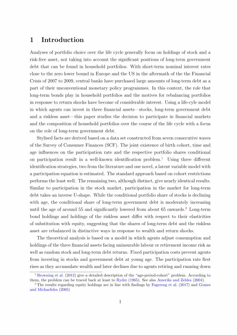
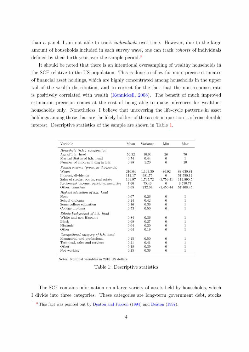
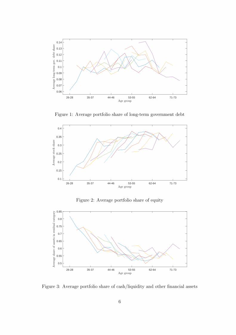
The figures 1-3 illustrate the average shares of the portfolio categories constructed in

this way. Each line represents the average portfolio share of a given birth-year cohort at

a particular age. Since data points are available only every three years, both respondent

age and cohort (birth year) are divided into three-year intervals. For example, the earliest

data available are from 1989. The youngest age group considered includes households with

a “household head” aged 26-28.8 Individuals that are 26-28 of age in 1989 belong to the

birth-year cohort 1961-63. The 1961-63 cohort is sampled seven times between 1989 and

2007. Its members are aged 29-31 in 1992, 32-34 in 1995 and so on. In Figures 1-3, the

7 See EBRI Note “IRA Asset Allocation and Characteristics of the CDHP Population, 2005-2010”from May 2011, available at www.ebri.org/publications/notes.

8 In the SCF, the term “household” refers to a “primary economic unit”, which consists of a core coupleor economically-dominant individual and other individuals that are financially interdependent with thatcouple or individual. The “household head” is defined as the single economically-dominant individual ina household without a core couple, the male in a household with a mixed-sex core couple and the olderindividual in the case of a same-sex core couple.

5

26-28 35-37 44-46 53-55 62-64 71-73

0.06

0.07

0.08

0.09

0.1

0.11

0.12

0.13

0.14

Figure 1: Average portfolio share of long-term government debt

26-28 35-37 44-46 53-55 62-64 71-73

0.1

0.15

0.2

0.25

0.3

0.35

0.4

Figure 2: Average portfolio share of equity

26-28 35-37 44-46 53-55 62-64 71-73

0.5

0.55

0.6

0.65

0.7

0.75

0.8

0.85

Figure 3: Average portfolio share of cash/liquidity and other financial assets

6

lines most to the left represent the average portfolio shares held by the 1961-63 cohort.

Similarly, the lines starting with age group 29-31 represent the average portfolio shares

of the 1958-60 cohort. Altogether, the sample contains the eleven cohorts born between

1931-33 and 1961-63, each observed at seven consecutive age groups between the ages of

26-28 and 74-76.9

The average portfolio share of stocks is increasing in household portfolios with a peak in

the late fifties or early sixties of the household head. Average long-term government debt

holdings behave in a somewhat similar way, although the pattern is less well pronounced.

The average portfolio share of the residual category follows a pattern that is markedly

distinct from that of the average long-term government bond share. However, it is a

well-known fact the averages computed in Figures 1-3 provide a biased picture of the

composition of household portfolios. The reasons are twofold.

First, the adjustments visible in the figures can be due to changes at the intensive or

extensive margin. A number of papers report that the rate of participation in the stock

market first increases and later decreases significantly over the life cycle.10 This suggests

that the inverse U-shape in Figure 2 largely results from households entering and exiting

the stock market rather than adjustments at the intensive margin. An important question

explored below is whether or not the same is true for holdings of long-term government

debt. The figures A.1 to A.3, which plot the participation rates in the data, provide first

suggestive evidence for the importance of adjustments at the extensive margin.

Second, as discussed in Ameriks and Zeldes (2004), it is not possible from the figures

to disentangle the effects of age, observation period and cohort. Age effects are related

to education, family formation and retirement. Period effects result from events that

occur at the time of data collection. For example, the dot-com-bubble and its bursting is

reflected in the survey waves from 2001 and 2004. Cohort effects include cohort-specific

experiences like growing up during war time as was the case for the oldest cohorts in the

sample. Even if, for example, we were to observe a figure of the same kind as Figures 1-3

in which all lines were perfectly aligned such that they formed one single upward-sloping

line, we could not say whether this was due to pure age effects or a combination of time

and cohort effects.11

9 Only cohorts that fall inside this age interval at all seven survey waves are considered. Younger andolder age groups are not examined due to a lack of sufficient data. Table A.2 in the Appendix showsthe number of observations for each cohort-age pair. The data set contains multiple imputations as isexplained in more detail in the table notes.

10 See Ameriks and Zeldes (2004), Fagereng et al. (2017) and Guiso et al. (2003). Haliassos (2008)contains a more general summary of the literature on limited participation in asset markets.

11 Time effects could cause each individual line to be sloped upwards and cohort effects of increasingsize could result in all lines aligning precisely in the way previously mentioned.

7

2.2 Identification

As outlined above, identification problems arise from sample selection and perfect multi-

collinearity of a respondent’s cohort, the age at which they are sampled and the year in

which the survey is conducted (birth year + age = observation period). An unresolved

issue in the literature on equity holdings over the life cycle is that estimation results are

somewhat dependent on the underlying identifying assumptions.12 I therefore present the

results obtained under three different identification strategies. Two are borrowed from the

literature and one is novel. A number of robust findings emerge. To be able to motivate

the strategies employed below, the nature of the identification problem is laid out before

in detail.

2.2.1 Sample Selection

The self-selection of agents into participants and non-participants in the market for a given

financial asset results in a sample selection problem. If agents enter and exit systematically

over the course of the life cycle, the age effects on the conditional portfolio share are

estimated with bias. To address this issue, I employ a standard latent variable model

with a Probit selection equation. Formally, the model is given by

si = x′2,iβ2 + σ12λ(x′1,iβ1

)+ e2,i (1)

∀i where si > 0 is i’s portfolio share of the asset in question, λ ≡ φ(x′1,iβ1

)/Φ(x′1,iβ1

)is the Inverse Mills Ratio and β1 is obtained from estimating the first-stage Probit model

Pr(Pi = 1|x1,i) = Pr(x′1,iβ1 + e1,i > 0

)= Φ

(x′1,iβ1

)(2)

Pi = 1 if i is a participant in the market for the asset considered and Pi = 0 otherwise.

The error terms are normal, e1,i ∼ N(0, 1) and e2,i ∼ N(0, σ2), with Cov(e1,i, e2,i) = σ12.

2.2.2 The “Age-Period-Cohort Problem”

Due to the multicollinearity described above, a simple linear model that aims to separate

age, period and cohort effects is under-identified. To see this, consider the following exam-

ple.13 Let ai denote the age of respondents, ti the time period in which they are sampled

12 See Ameriks and Zeldes (2004) and Gomes and Michaelides (2005) for detailed discussions.13 See also Browning et al. (2012).

8

and ci their year of birth. Suppose that observations are available for two consecutive

time periods, ti ∈ t1, t2, and that three consecutive cohorts are sampled in both periods,

ci ∈ c1, c2, c3. Age can then take on four distinct values, ai ∈ a1, a2, a3, a4.14

A projection of some variable of interest yi on age, period and cohort indicators is

yi = α1a1i + α2a

2i + α3a

3i + α4a

4i

+ θ2t2i

+ γ2c2i + γ3c

3i + ei (3)

where xni = 1 if xi = xn and xni = 0 otherwise for x ∈ a, t, c and n ∈ 1, 2, 3, 4.Note that t1i , c

1i and a constant have been omitted to prevent each set of binary variables

from summing to the constant. However, the fact that there exists a linear relationship

between the age, observation period and cohort of each respondent implies that the data

matrix pertaining to equation (3) is not invertible and that parameter estimates cannot

be computed using standard methods. More precisely, the linear relationship between

age, period and cohort implies15

2a1i + a2

i − a4i + t2i = c2

i + 2c3i (4)

Inserting (4) into (3) yields

yi = α1a1i + α2a

2i + α3a

3i + α4a

4i

+ γ2c2i + γ3c

3i + ei (5)

where

α1

α2

α3

α4

γ2

γ3

=

1 0 0 0 −2 0 0

0 1 0 0 −1 0 0

0 0 1 0 0 0 0

0 0 0 1 1 0 0

0 0 0 0 1 1 0

0 0 0 0 2 0 1

α1

α2

α3

α4

θ2

γ2

γ3

(6)

14 For example, if ti ∈ 2000, 2001 and ci ∈ 1950, 1951, 1952 then ai ∈ 48, 49, 50, 51.15 Continuing the previous example, a person that is born say in 1952 and surveyed in 2001 is aged 49

when surveyed; thus t2i = c3i = a2i = 1 and a1i = a4i = c2i = 0. It is straight forward to verify that (4)holds for all six such combinations of binary-variable values for which the birth year and the age sum tothe observation period.

9

Using equation (5), one can estimate the six reduced form parameters α1, α2, α3, α4, γ2, γ3.

From (6) it is clear though that it is not possible to solve for the seven structural pa-

rameters α1, α2, α3, α4, θ2, γ2, γ3 knowing the reduced form parameters. The structural

parameters are under-identified, unless at least one parameter restriction is imposed. It

can be easily shown that this result generalises to scenarios with more observation periods

and cohorts.

To be able to judge the robustness of the estimation results, I pursue three distinct

identification strategies. The first and most standard is to impose an equality restriction

on neighbouring cohort effects, i.e. to impose

γn = γn+1 (7)

for some n. This restriction formally reduces the generality of the model, yet the bias it

introduces should be expected to be small if two neighbouring cohorts can be identified

that have a sufficiently similar history.

The second strategy was suggested by Deaton and Paxson (1994) and more recently

used by Fagereng et al. (2017) among others. The idea is to attribute cyclical fluctuations

to time effects and trends to age and cohort effects. This is achieved by requiring time

effects to sum to zero and to be orthogonal to a linear time trend, that is

g′θ = 0 (8)

where g = (0, 1, ..., T −1)′ is the trend, θ is the vector of coefficients on the time dummies

and T is the number of observation periods. This set of restrictions correctly identifies all

effects if indeed only age and cohort effects are trending. In the context here, one cannot

be sure however that there is no trend in time effects. In particular, in the time period

examined (1989-2007), stocks became a more widely-used mode of saving. Imposing (8)

when a trend in time effects is present in the data could cause the coefficients on the age

and cohort variables to jointly pick up this trend and therefore to be biased. In the second-

stage regression, I therefore follow Fagereng et al. (2017) in de-trending the dependent

variable, the portfolio share of a given asset, by subtracting its cross-sectional average at

each time period. Since this is not feasible in a binary dependent variable model, I add

a linear time trend as an explanatory variable at the first stage. This implies that one

additional dummy has to be excluded from the Probit model.

Under the final identification strategy, the time dummies are replaced with the first p

principal components of a large set of stationary macroeconomic time series covering the

10

entire sample period. This resolves the linear dependence of the independent variables. As

before, the asset share is de-trended and a trend is added to the selection equation. To the

extent that the principal components contain the effects otherwise picked up by the time

dummies, this modification allows controlling for age, period and cohort effects without

parameter restrictions. In particular, institutional and regulatory changes concerning the

usage of different savings instruments can be expected to be reflected in asset prices and

interest rates. Note that to provide a meaningful addition to the previous identification

approach, p should not be chosen too large.16

2.3 Estimation and Results

Beginning with the second-stage regression, the equations estimated in case of the first

identification strategy (parameter restriction on cohort effects) are

si = a′iα2 + t′iθ2 + c′iγ2 + ςλi + z′2,iδ2 + e2,i (9)

Pr(Pi = 1|x1,i) = Φ(a′iα1 + t′iθ1 + c′iγ1 + z′1,iδ1

)(10)

ai =(a26−28i , a29−31

i , . . . , a74−76i

)′is a complete set of age dummies for seventeen age groups,

ti = (t1992i , t1995

i , . . . , t2007i )

′is a vector of six year dummies and ci =

(c1934−36i , c1937−39

i , . . . ,

c1961−63i

)′contains a dummy for each of ten cohorts. z2,i and z1,i are additional household-

specific controls and x1,i ≡ (ai, ti, ci, z1,i)′. In the case of the other two strategies, the

equations are modified as explained in the previous section. Information on the controls

used in the estimation and a detailed discussion of the exclusion restrictions imposed in

the second step of the selection model are contained in Section D of the Appendix.

Figure 4 plots the estimation results for all three identification strategies outlined

before including separate sets of results for two different cohort restrictions. The first

cohort restriction equates the effects of the two oldest cohorts in the sample, 1934-36 and

1937-39, the second one those from the first two post-war cohorts, 1946-48 and 1949-51.

The cohort effects of the oldest respondents are equated, since it seems likely for any

differences between them to wash out over the years until the sampling period and the

second restriction may appear reasonable from a historical perspective. In the model in

which the time dummies are dropped, the first p = 3 principal components of a large

16 Suppose a model with Deaton-Paxson restrictions contains T ′ time dummies, which, together with thetwo constraints that the time effects be orthogonal to a linear trend and sum to zero, can be summarisedby T ′− 2 variables constructed in an appropriate way. Then, if the principal components included underthe final identification strategy are also approximately orthogonal to a linear trend and mean zero, amodel with p ≥ T ′ − 2 principal components spans the same space as the one with time dummies andDeaton-Paxson restrictions. To avoid this case, it is ensured in the estimation below that p < T ′ − 2.

11

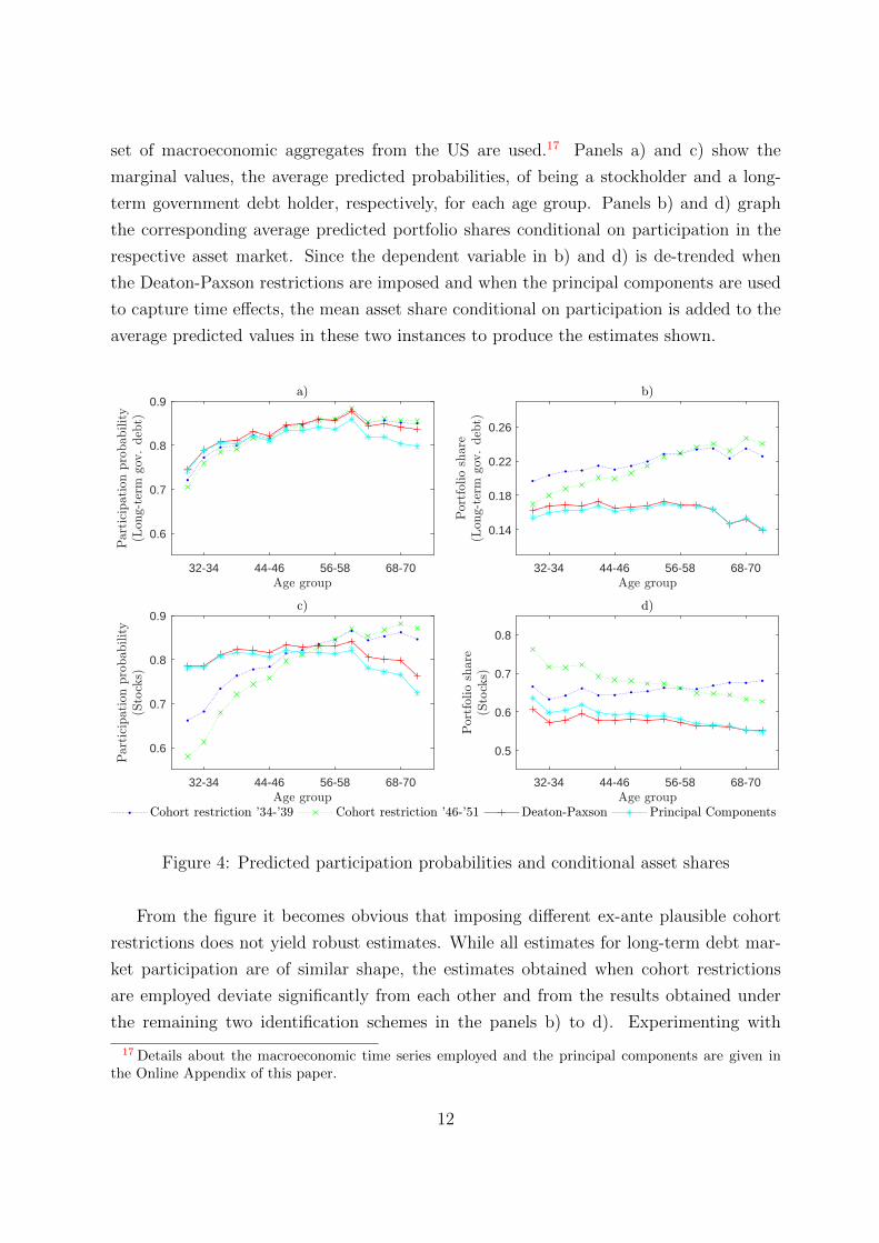
set of macroeconomic aggregates from the US are used.17 Panels a) and c) show the

marginal values, the average predicted probabilities, of being a stockholder and a long-

term government debt holder, respectively, for each age group. Panels b) and d) graph

the corresponding average predicted portfolio shares conditional on participation in the

respective asset market. Since the dependent variable in b) and d) is de-trended when

the Deaton-Paxson restrictions are imposed and when the principal components are used

to capture time effects, the mean asset share conditional on participation is added to the

average predicted values in these two instances to produce the estimates shown.

32-34 44-46 56-58 68-70

0.6

0.7

0.8

0.9

32-34 44-46 56-58 68-70

0.14

0.18

0.22

0.26

32-34 44-46 56-58 68-70

0.6

0.7

0.8

0.9

32-34 44-46 56-58 68-70

0.5

0.6

0.7

0.8

Figure 4: Predicted participation probabilities and conditional asset shares

From the figure it becomes obvious that imposing different ex-ante plausible cohort

restrictions does not yield robust estimates. While all estimates for long-term debt mar-

ket participation are of similar shape, the estimates obtained when cohort restrictions

are employed deviate significantly from each other and from the results obtained under

the remaining two identification schemes in the panels b) to d). Experimenting with

17 Details about the macroeconomic time series employed and the principal components are given inthe Online Appendix of this paper.

12

different cohort restrictions showed that the discrepancies are even more severe for other

pairs of economically plausible restrictions, likely because trends in the cohort effects not

accounted for by the model are forced into the estimates of the age effects. However,

the results obtained using Deaton-Paxson restrictions and principal components nearly

coincide despite of their distinct way of accounting for time influences and are consistent

with previous findings about equity holdings from the literature.18

Several stylised facts emerge from the estimations that make use of Deaton-Paxson

restrictions or principal components. The profile of participation in the market for long-

term government debt shows a pronounced hump shape. Participation rates rise over the

course of nearly the entire working life and then begin to decline at the age of 62-64 as

household members retire. The age effects on the conditional portfolio share of long-term

government debt are mildly increasing at first and roughly constant from the mid-forties

until retirement. A significant decline is not observable until after the age of 65. Overall,

the results suggest that there is a clear inverse U-shape in participation rates and that the

conditional portfolio share is non-decreasing until retirement, but falls thereafter. Stock

market participation takes an almost identical shape to participation in the market for

long-term government debt. The conditional stock share is monotone declining from 39-41

onwards.

The life-cycle dynamics of stock-market participation and the conditional share of

stocks have been a topic of debate in the literature. In summarising the existing empirical

evidence, Gomes and Michaelides (2005) state that 1) stock-market participation increases

over the working life, 2) there is some evidence which suggests that participation rates

decline after retirement and 3) there is “no clear pattern of equity holdings over the life

cycle”. I interpret the results presented here as support for 1) and 2). In recent work,

Fagereng et al. (2017) find evidence for the conditional stock share to decline over the life

cycle using administrative panel data from the Norwegian Tax Registry.19 Regarding 3),

my estimates are more in line with their findings.20

Table 2 provides more detailed information about the estimations for the long-term

debt share. The results from the models with cohort restrictions are included for compar-

ison purposes. The coefficient on the inverse Mills ratio λ is significant and the correlation

of first-stage and second-stage residuals ρ is estimated to be positive, confirming the need

to address the selection problem. SCF data are multiply imputed. The size of the smallest

18 The estimated cohort and time effects are shown in the Online Appendix.19 Considering cross-sectional data only, other studies conclude that the conditional equity share may

be mildly increasing or also mildly hump-shaped. See Campanale et al. (2015) for a short discussion.20 In the Online Appendix it is shown that the stylised facts are robust to reassigning corporate bond

holdings to the long-term debt category.

13

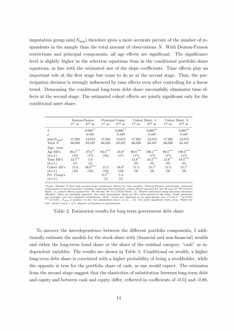
imputation group min(Nimp) therefore gives a more accurate picture of the number of re-

spondents in the sample than the total amount of observations N . With Deaton-Paxson

restrictions and principal components, all age effects are significant. The significance

level is slightly higher in the selection equations than in the conditional portfolio share

equations, in line with the estimated size of the slope coefficients. Time effects play an

important role at the first stage but cease to do so at the second stage. Thus, the par-

ticipation decision is strongly influenced by time effects even after controlling for a linear

trend. Demeaning the conditional long-term debt share successfully eliminates time ef-

fects at the second stage. The estimated cohort effects are jointly significant only for the

conditional asset share.

Deaton-Paxson Principal Comp. Cohort Restr. 1 Cohort Restr. 21st st. 2nd st. 1st st. 2nd st. 1st st. 2nd st. 1st st. 2nd st.

λ 0.065** 0.066** 0.065** 0.065**

ρ 0.445 0.449 0.445 0.445

min(Nimp) 17,202 12,673 17,202 12,673 17,202 12,673 17,202 12,673Total N 86,030 63,437 86,030 63,437 86,030 63,437 86,030 63,437

Sign. tests

Age Eff’s 96.4*** 27.6** 82.4*** 25.9* 96.8*** 106.1*** 99.2*** 108.5***

(d.o.f.) (16) (17) (16) (17) (17) (17) (17) (17)

Time Eff’s 12.7** 5.9 12.8** 43.3*** 12.8** 44.5***

(d.o.f.) (5) (5) (6) (6) (6) (6)

Cohort Eff’s 11.6 26.0*** 11.7 16.9* 11.5 15.1* 11.5 15.1*

(d.o.f.) (10) (10) (10) (10) (9) (9) (9) (9)

Pri. Comp’s 9.5** 5.4(d.o.f.) (3) (3)

Notes: Results of first and second stage estimation shown for four models—Deaton-Paxson restrictions, principalcomponents of macroeconomic variables replacing time dummies, cohort effects equated for ’34-’36 and ’37-’39 (CohortRestr. 1), cohort effects equated for ’46-’48 and ’49-’51 (Cohort Restr. 2). Models estimated using two-step estimator(Heckit). Data are multiply imputed. For each respondent, there are five observations in the data. Point estimatesare averages over five separate estimations. Strd. errors are adjusted in an appropriate way (∗p<0.1, ∗∗p<0.05,∗∗∗p<0.01). Nimp is number of obs. for imputation imp ∈ 1, 2, ..., 5. For joint significant tests, avrg. Wald test

stat. shown (each ∼ χ2), degrees of freedom in parentheses.

Table 2: Estimation results for long-term government debt share

To uncover the interdependence between the different portfolio components, I addi-

tionally estimate the models for the stock share with (financial and non-financial) wealth

and either the long-term bond share or the share of the residual category “cash” as in-

dependent variables. The results are shown in Table 3. Conditional on wealth, a higher

long-term debt share is correlated with a higher probability of being a stockholder, while

the opposite is true for the portfolio share of cash, as one would expect. The estimates

from the second stage suggest that the elasticities of substitution between long-term debt

and equity and between cash and equity differ, reflected in coefficients of -0.52 and -0.88,

14

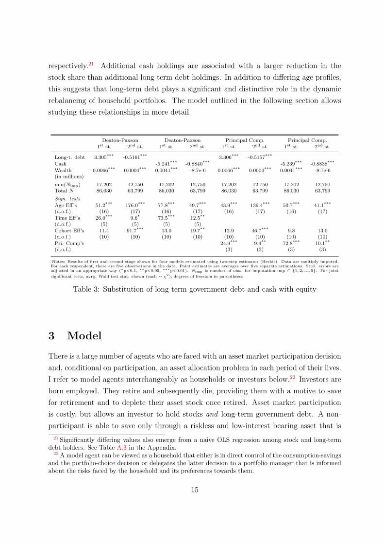
respectively.21 Additional cash holdings are associated with a larger reduction in the

stock share than additional long-term debt holdings. In addition to differing age profiles,

this suggests that long-term debt plays a significant and distinctive role in the dynamic

rebalancing of household portfolios. The model outlined in the following section allows

studying these relationships in more detail.

Deaton-Paxson Deaton-Paxson Principal Comp. Principal Comp.1st st. 2nd st. 1st st. 2nd st. 1st st. 2nd st. 1st st. 2nd st.

Long-t. debt 3.305*** -0.5161*** 3.306*** -0.5157***

Cash -5.241*** -0.8840*** -5.239*** -0.8838***

Wealth 0.0066*** 0.0004*** 0.0041*** -8.7e-6 0.0066*** 0.0004*** 0.0041*** -8.7e-6(in millions)

min(Nimp) 17,202 12,750 17,202 12,750 17,202 12,750 17,202 12,750Total N 86,030 63,799 86,030 63,799 86,030 63,799 86,030 63,799

Sign. tests

Age Eff’s 51.2*** 176.0*** 77.8*** 49.7*** 43.9*** 139.4*** 50.7*** 41.1***

(d.o.f.) (16) (17) (16) (17) (16) (17) (16) (17)

Time Eff’s 26.0*** 9.6* 73.5*** 12.5**

(d.o.f.) (5) (5) (5) (5)

Cohort Eff’s 11.4 91.7*** 13.0 19.7** 12.9 46.7*** 9.8 13.0(d.o.f.) (10) (10) (10) (10) (10) (10) (10) (10)

Pri. Comp’s 24.9*** 9.4** 72.8*** 10.1**

(d.o.f.) (3) (3) (3) (3)

Notes: Results of first and second stage shown for four models estimated using two-step estimator (Heckit). Data are multiply imputed.For each respondent, there are five observations in the data. Point estimates are averages over five separate estimations. Strd. errors areadjusted in an appropriate way (∗p<0.1, ∗∗p<0.05, ∗∗∗p<0.01). Nimp is number of obs. for imputation imp ∈ 1, 2, ..., 5. For joint

significant tests, avrg. Wald test stat. shown (each ∼ χ2), degrees of freedom in parentheses.

Table 3: Substitution of long-term government debt and cash with equity

3 Model

There is a large number of agents who are faced with an asset market participation decision

and, conditional on participation, an asset allocation problem in each period of their lives.

I refer to model agents interchangeably as households or investors below.22 Investors are

born employed. They retire and subsequently die, providing them with a motive to save

for retirement and to deplete their asset stock once retired. Asset market participation

is costly, but allows an investor to hold stocks and long-term government debt. A non-

participant is able to save only through a riskless and low-interest bearing asset that is

21 Significantly differing values also emerge from a naive OLS regression among stock and long-termdebt holders. See Table A.3 in the Appendix.

22 A model agent can be viewed as a household that either is in direct control of the consumption-savingsand the portfolio-choice decision or delegates the latter decision to a portfolio manager that is informedabout the risks faced by the household and its preferences towards them.

15

comparable to short-term bonds or cash. Thus, agents who choose to invest in only one of

the two risky assets have to incur the entire asset market participation cost.23 Investors

are subject to uninsurable idiosyncratic and aggregate risk. Idiosyncratic risk arises from

non-financial income and aggregate risk results from the returns on stocks and long-term

government debt.

3.1 Life Cycle Stages

Each investor i ∈ I lives for T periods and goes through an employment and a retirement

stage. Investors are born employed at the beginning of period t = 1, retire in period

Tret > 1 and die at the end of period T > Tret. Note that the model describes the

decisions of a large number of agents belonging to the same generation and that, as

a result, there is no interaction between different, potentially overlapping, generations.

Investors supply labour inelastically as long as they remain employed, which entitles them

to an exogenous income stream given by

Yi,t = Pi,tUi,t, lnUi,t ∼ N(−0.5σ2u, σ

2u) (11)

Pi,t = GPi,t−1Ni,t, lnNi,t ∼ N(−0.5σ2n, σ

2n) (12)

Labour income has a transitory component Ui,t and a persistent component Pi,t.24 The

logarithm of Pi,t follows a random walk with drift. The expectation of the shock to the

persistent component of income Ni,t and the expectation of the transitory shock Ui,t equal

one, so that, in expectation, the labour income of all agents grows at the common rate

G − 1.25 Retired investors receive a pension Ωi,t = ωPi,Tret which is a fraction of the

persistent income that they obtained in the last period in which they were employed as

in the model of Gomes and Michaelides (2005) among others. This specification captures

the empirical fact that differences in income that develop over the course of the working

life persist among retired investors.

23 The model does not include separate participation costs for the long-term government debt marketand the stock market to reduce the dimensionality of the portfolio choice problem. Participation inboth markets is highly correlated in the sample with a coefficient of 0.80 and Figure 4 suggests thatthis simplification yields a good approximation of observed household behaviour. Figure A.8 shows thatre-estimating the empirical models with a joint asset-market participation decision does not alter thestylised facts described in the previous section.

24 This income process is frequently used in the literature and originally due to Carroll et al. (1992).They refer to P somewhat ambiguously as “permanent labour income”.

25 In general, if lnx ∼ N(µ, σ), then Ex = exp(µ+ 0.5σ2

), therefore EUi,t = ENi,t = 1.

16

3.2 Investment Opportunities

There are three types of assets available to the investors: a one-period bond, stocks and

long-term government debt. Long-term government debt has a maturity of δ periods.

A strategy frequently adopted in the literature is to assume that long-term bonds are

entirely illiquid, or more precisely, that they have to be held until maturity. Aside from

understating the liquidity of long-term government debt, this assumption leads to a big

inflation of the state space as δ becomes large, causing exact solutions to portfolio choice

problems to be computationally burdensome. A specification is proposed here that, in

accordance with the US long-term bond market, allows investors to access some of the

funds held in the form of long-term debt in each period and that makes the portfolio

optimisation computationally feasible.

An investor that has purchased long-term government bonds in period t − 1 at the

amount of Qi,t−1 receives a Calvo-type signal for each infinitesimal unit of rq,tQi,t−1 in

period t indicating whether it can be sold or not. rq,t is the annual gross return on the

long-term government bond. A positive signal is received with probability δ−1, implying

that each infinitesimal unit has to be held on average for δ periods. Thus, portfolios are

chosen in all periods subject to the constraint

Qi,t ≥ (1− δ−1)rq,tQi,t−1 (13)

Comparable to the case in which long-term bonds have to be held until maturity, the

minimum expected holding period of the entire stock is equal to its maturity, but a

fraction of this stock can be accessed in each period. Since the probability of being

able to sell a given unit of long-term debt is time-constant, all long-term debt held by i

can be summarised by one single state variable. Modelling long-term government bonds

as a perpetuity as in Woodford (2001) would equally permit all long-term debt to be

represented by a single state variable. However, the specification chosen here emphasises

the imperfect liquidity of long-term government debt, which is an important characteristic

of assets such as US savings bonds and tax-exempt bonds.26

The one-period bond yields the riskless gross return rb. Following Bonaparte et al.

(2012), the gross stock return rs,t evolves according to a two-state Markov process, rs,t ∈rls, r

hs

, with mean rs and standard deviation σrs. Accounting for capital gains and

26 The two specifications are similar though. For a perpetuity, the pay-off stream from a one-dollarinvestment is ρ, ρ2, ρ3, . . . for some ρ ∈

[0, β−1

). Here, if government debt is run down at the fastest

possible rate, this stream is (1 − δ−1)rq,t+1, (1 − δ−1)2rq,t+1rq,t+2, (1 − δ−1)3rq,t+1rq,t+2rq,t+3, . . . with(1− δ−1) ∈ [0, 1).

17

dividends, Bonaparte et al. cannot reject that the annual stock return in the US is

serially uncorrelated. rs,t is therefore assumed to be i.i.d. across periods with probabilities

of a half for both return states. The return on long-term government debt equally follows

a two-state Markov process. The mean, the standard deviation and the transition matrix

are given by rq, σrq and Γrq, respectively. No restrictions are placed on Γrq, allowing for

persistence in the government bond return process.

Holdings of the short-term bond Bi,t are costless. Investments in stocks Si,t and long-

term government debt Qi,t are associated with a cost of size Ψi,t = ψPi,t if i is employed

and Ψi,t = ψPi,Tret if i is retired that has to be paid in each period of active participation

in the markets for stocks or long-term government debt. Ψi,t represents, for example,

costs associated with the acquisition of information about financial markets and is scaled

to the persistent component of income in order to capture the opportunity cost of time.27

Investors are not considered active participants in financial markets if they hold no stocks

and allow potential previously-acquired holdings of long-term bonds to mature at the

fastest possible rate. Thus, if the investor chooses not to pay Ψi,t, Si,t = 0 and (13) holds

with equality.28 In addition, stock holdings are subject to a variable cost ψsSi,t, reflecting

the monetary costs of maintaining a stock portfolio. The role played by the two types of

costs is re-visited below in more detail.

3.3 Optimisation Problem

The optimal plan of investor i ∈ I solves the problem described in this section in each

period t = 1, 2, . . . , T . The indices i and t are suppressed below for notational clarity.

3.3.1 Financial-Market Participants

The budget constraint of an investor that participates in financial markets is given by

C + S(1 + ψs) +B +Q+ Ψ = rsS−1 + rbB−1 + rqQ−1 + Θ (14)

27 In Alan (2006), the cost of stock-market participation is equally made dependent on the persistentcomponent of labour income, however, it is incurred only the first time an agent enters the market andnot, for example, at a later re-entry.

28 If non-participants were able to reduce long-term bond holdings at a faster rate, there would beliquidity gains associated with not acquiring information about financial markets. If they were able toreduce long-term bond holdings at a slower rate, the expected average holding period of long-term bondswould be larger than the maturity of the bond. Therefore, the assumption that (13) must hold withequality for non-participants seems most plausible.

18

where non-financial income Θ ∈ Y,Ω equals Y if the investor is employed and Ω oth-

erwise. The sum of expenditures on consumption, stocks, short-term bonds, long-term

government debt and all costs incurred must be equal to income, which is given by the

gross return on last period’s investments and non-financial income.

Defining “cash on hand” as

X ≡ rsS−1 + rbB−1 + δ−1rqQ−1 + Θ (15)

and illiquid assets as

Z ≡ (1− δ−1)rqQ−1, (16)

one can express the budget constraint as

C + S(1 + ψs) +B +Q+ Ψ = X + Z (17)

In equation (17), income is divided into liquid funds X that can be freely allocated

towards all types of expenditures and illiquid funds Z which are tied to a re-investment

in long-term government debt. Using this notation, the liquidity constraint on long-term

government (13) debt becomes

Q ≥ Z (18)

requiring investors to carry an amount of long-term debt forward into the next period

that is at least as large as the amount of illiquid assets brought into the period.

In the event of participation in the current period, the optimal portfolio choice satisfies

vp (X,Z, rq, P, t) = maxC,S,B,Q

u(C) + βEU ′,P ′,r′s,r′q |P,rqv

(X ′, Z ′, r′q, P

′, t+ 1)

(19)

together with (15)-(18) and the regularity conditions (S,B,Q) ≥ (S,B,Q). Here, u :

R+ → R is the period utility function with u′(C) > 0 and u′′(C) < 0 for all C ∈ R+,

vp : R2 × (R+)2 × N → R is the indirect utility function conditional on financial-market

participation in the current period and v is unconditional indirect utility derived below.

Since retirement income is deterministic, the expectation has to be taken over U ′ and P ′

only if the investor is employed.

19

3.3.2 Financial-Market Non-Participants

The budget constraint of a household that does not participate in financial markets is

C +B +Q = rsS−1 + rbB−1 + rqQ−1 + Θ

= X + Z (20)

As discussed before, for a non-participant

Q = Z (21)

which implies that the budget constraint can be written as

C +B = X (22)

The equation above is independent of Q, reflecting the fact that the only choice that a

non-participant faces is how to allocate cash on hand towards consumption and savings

at the risk-free rate.

In this case, the solution must satisfy

vn (X,Z, rq, P, t) = maxC,B

u(C) + βEU ′,P ′,r′q |P,rqv(X ′, Z ′, r′q, P

′, t+ 1)

(23)

as well as (15), (16), (20), (21) and B ≥ B, where vn : R2 × (R+)2 × N → R gives

indirect utility if the household does not participate and retired agents face no risk from

non-financial income as explained above.

3.3.3 Participation Decision

In each period, an investor has to decide whether or not to participate in financial markets

having solved the consumption-savings problem and the portfolio choice problem in the

case of participation. The value of the problem of an investor is given by

v (X,Z, rq, P, t) = max vp (X,Z, rq, P, t) , vn (X,Z, rq, P, t) (24)

At each point in the state space, the investor decides to participate in financial markets

if the value from participating is higher than that from not participating.

20

3.4 Computation

The model has to be solved numerically. The fact that agents are able to invest in a

third financial asset with a persistent stochastic return increases the dimensionality of the

problem significantly in comparison to other recent models of portfolio choice over the

life cycle.29 There are three continuous state variables in addition to the prevailing level

of the return on long-term debt and the investors’ age. The optimisation involves four

continuous controls. One state variable can be eliminated from the problem by dividing

all endogenous variables by the persistent component of labour income P . Below, lower

case letters denote normalised variables, e.g. x ≡ X/P . Period utility is assumed to be

of CRRA form with a coefficient of relative risk aversion γ. This implies that all value

functions introduced above are homogeneous of degree 1 − γ. For example, the indirect

utility of an employed investor that participates in financial markets in the current period

can be expressed as

vp (x, z, rq, t) = maxc,s,b,q

u(c) + βEU ′,N ′,r′q ,r′s|rq (GN ′)

1−γv(x′, z′, r′q, t+ 1

)(25)

The stochastic growth rate of the persistent component of income P ′/P = GN ′ raised to

1−γ now pre-multiplies v in the expected value accounting for uncertainty resulting from

persistent income shocks. All normalised model equations together with more details on

their derivation are listed in Section E of the Appendix.

3.5 Calibration

Table 4 shows the calibration used for the simulations presented in the sections that follow.

Note that the model is written entirely in real terms. A period corresponds to a year. Since

the age group 26-28 is the youngest contained in the estimations described in Section 2, it

is assumed that agents are born at the age of 27. Tret and T are selected such that agents

retire just before turning 63 years of age and die at the age of 80, respectively, consistent

with data from the US Census Bureau. A value of five for δ implies that the long-term

bond approximates 5-year government debt. This is in line with the average maturity

of all outstanding marketable securities issued by the US Treasury which averaged 59.7

months between January 2000 and December 2007.30

As in Bonaparte et al. (2012) and Campanale et al. (2015), the risk-free rate is set to

29 Examples of models with two assets include Bonaparte et al. (2012), Campanale et al. (2015) andCocco et al. (2005).

30 Between January 2000 and March 2016 the average debt maturity was 60.7 months.

21

2%, a value that is commonly used in the literature. Bonaparte et al. further estimate

the average net return of stocks in the US, inclusive of dividend payments, to be 6.33%

with a a standard deviation of 0.155 and no serial correlation, which I also adopt here.

The mean excess return of 5-year government debt over the risk-free rate is set to 0.6%,

the standard deviation of 5-year US debt over the sampling period was about 0.011.

The 5-year government debt return is modelled using a two-state Markov process whose

transition matrix is found by first fitting an AR(1) process to the data and then finding

the transition probabilities that best describe the estimated AR(1) process as proposed

in Hussey and Tauchen (1991). rq remains in state k ∈ l, h with probability 0.663 and

switches with the converse probability.

Parameter Value Description Target/Source

Tret 36 Retirement period Avrg. US retirement ageT 54 Death period US life expectancyδ 5 Maturity of government debt Avrg. maturity of marketable US debtβ 0.96 Discount factor Gomes and Michaelides (2005)γ 5 Coefficient of relative risk aversion Gomes and Michaelides (2005)σu 0.16 SD of log transitory income shock Carroll et al. (1992)σn 0.12 SD of log persistent income shock Carroll et al. (1992)G 1.03 Mean income growth Haliassos and Michaelides (2003), Viceira (2001)ω 0.6 Replacement ratio Campanale et al. (2015), Munnell and Soto (2005)rb 1.02 Gross return of riskless bond Bonaparte et al. (2012)rs 1.0633 Mean gross stock return Bonaparte et al. (2012)σrs 0.155 SD of stock return Bonaparte et al. (2012)rq 1.026 Mean gross return of δ-year bond 5-year Treasury Notes returnσrq 0.011 SD of δ-year bond return 5-year Treasury Notes return

Γrq,kk 0.663 Pr(rkq |rkq ) for k ∈ l, h 5-year Treasury Notes returnψs 0.015 Variable cost of stock holdings Avrg. expense ratio of equity fundsψ 0.035 Participation cost parameter Campanale et al. (2015), Gomes and Michaelides (2005)

B, Q, S 0 Borrowing limits Campanale et al. (2015)

Table 4: Calibration

The standard deviations of the shocks to the transitory and the persistent component

of income are chosen based on the estimates reported in the seminal contribution by Car-

roll et al. (1992). Several papers draw on these results, including Gomes and Michaelides

(2005) and Haliassos and Michaelides (2003). Carroll et al. (1992) set income growth to

two per cent, subsequent papers use a slightly higher value of three per cent, which I follow

here (Haliassos and Michaelides, 2003; Viceira, 2001). The replacement ratio employed is

0.6 in line with Campanale et al. (2015) and Munnell and Soto (2005).31

31 Munnell and Soto (2005) find that, in the US, the replacement rate ranges from about 0.6 to 0.8for households covered by a pension plan and from about 0.45 to 0.6 for those without pension coveragedepending on the precise definitions used.

22

A number of authors that examine stock holdings over the life cycle report estimates

of the discount factor and the coefficient of relative risk aversion. Although the results

vary considerably, generally a relatively high degree of discounting and risk aversion is

required to match the data. The estimates of Bonaparte et al. (2012) are β = 0.69 and

γ = 7.24. Alan (2006) estimates β = 0.92 and γ = 1.6. Cagetti (2003) shows that both

variables strongly depend on education with estimates for groups of different education

levels ranging from 0.78 to 1.14 for β and from 2.40 to 8.13 for γ. Campanale et al. (2015)

employ β = 0.94 and γ = 5. Following Gomes and Michaelides (2005), I use standard

values of β = 0.96 and γ = 5.32

The high structural estimates for the discount rate and the coefficient of relative risk

aversion are related to a puzzle that poses a challenge to the literature on portfolio choice

over the life cycle. According to standard models, it is optimal for households to invest

a bigger share into high-risk and high-return assets like stocks than they do according to

survey data. A number of strategies have been employed to align model-based predictions

more closely with the empirical evidence. Calibrations with high, occasionally extreme

levels of discounting and risk aversion respectively lower the benefits from the high average

return and increase the sensitivity of households towards the high volatility of stocks.

Transaction costs which imply that investors cannot costlessly convert stock holdings into

consumption equally reduce the value of stock holdings for households (Campanale et al.,

2015). Disastrous labour income shocks occurring with a small probability make total

income, ceteris paribus, more risky and therefore lead households to reduce portfolio risk

by lowering the stock share. Finally, an isolated decrease in the elasticity of intertemporal

substitution, implemented by generalising CRRA utility to the Epstein-Zin-Weil recursive

form, causes households to increase savings and thus financial income which also implies

a lower optimal stock share.33

The focus of this paper lies on the dynamic patterns according to which liquidity,

long-term debt and stocks are substituted as wealth is accumulated and de-accumulated

with age rather than the effect that the addition of long-term debt to the portfolio choice

problem of households has on the mean level of stock holdings. To keep the analysis as

clean as possible, therefore merely two types of realistically-calibrated costs whose effects

are easily understood are included in the model. The fixed cost of asset-market partici-

32 As in Alan (2006) and Bonaparte et al. (2012), expected utility is discounted at a constant rate. Time-variation in the discount factor could be introduced through age-dependent conditional death probabilitieswhich according to data from the National Center for Health Statistics (NCHS) are small until old agethough.

33 See Cocco et al. (2005) for more details on the effects of disastrous labour income shocks and changesin the elasticity of intertemporal substitution.

23

pation ψ gives rise to a meaningful participation decision and the variable cost of stock

holdings ψs to an interior solution to the conditional asset allocation problem. Gomes and

Michaelides (2005) calibrate stock-market entry costs to 2.5% of the persistent component

of labour income, Alan (2006) estimates a value of about 2.1%. In the model of Bonaparte

et al. (2012), agents incur a transaction cost in each period in which stock holdings are

adjusted. Their estimate for these costs is 1.2% of total labour income. Campanale et al.

(2015) consider transaction costs that are comparable to those in Bonaparte et al. (2012)

which they calibrate to 4%-7%, depending on the level of education, in a their preferred

scenario. In accordance with these values, ψ is set to 3.5% here.

The Investment Company Institute (ICI) publishes data on the fees associated with

investments in equity funds, which I use as an approximation of the marginal cost of

holding a stock portfolio. The average expense ratio, the ratio of annual fees to the total

size of the investment, fell from 1.6% in 2000 to 1.5% in 2007 and 1.3% in 2015.34 Based

on these figures, a value of 1.5% is chosen for ψs. Following the literature the possibility

of borrowing and short selling is excluded in the model (Campanale et al., 2015).35

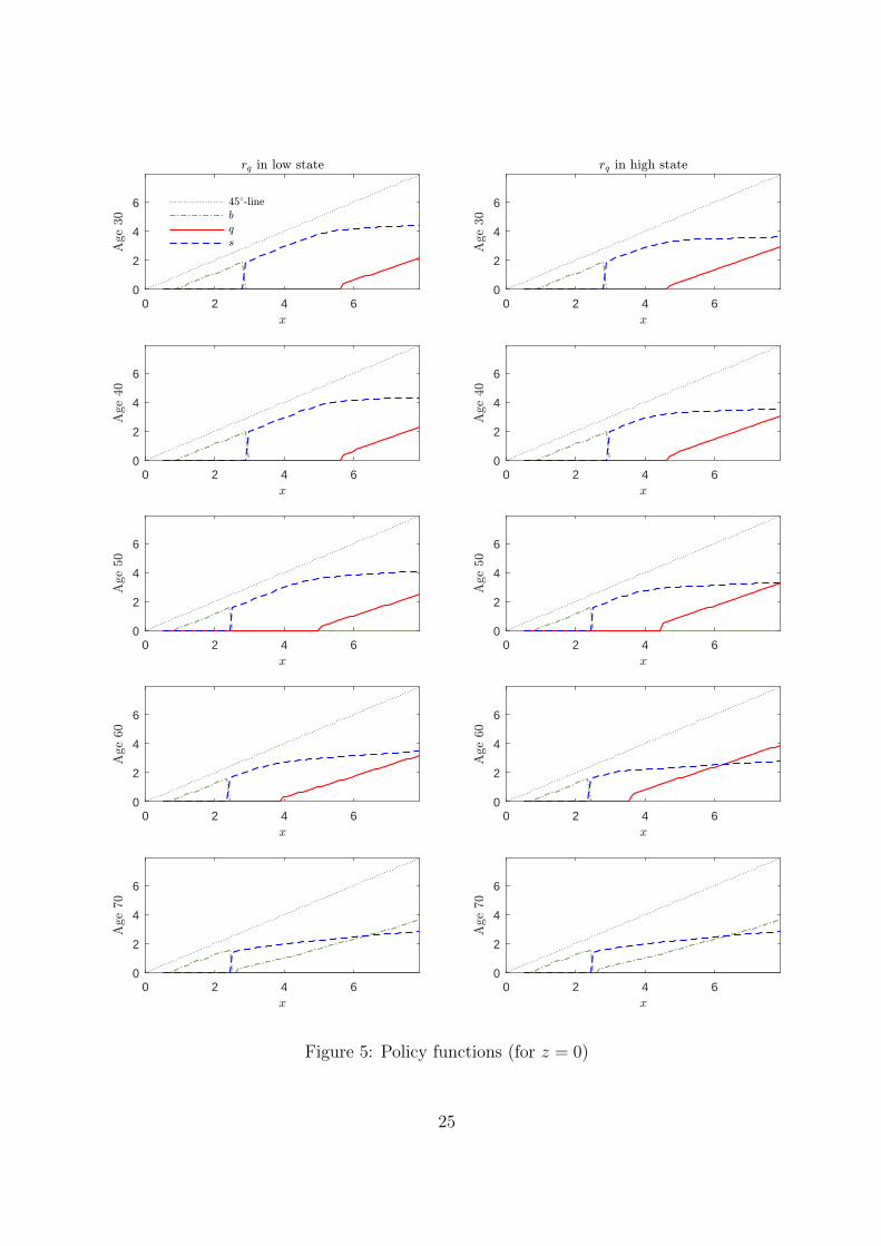
3.6 Portfolio Rebalancing

The policy functions associated with the optimisation problem laid out above illustrate

how investors rebalance their portfolios as financial wealth increases. In Figure 5, the

optimal choice of financial assets is plotted against cash on hand at different ages. Poten-

tial illiquid asset holdings brought into the period are set to zero for now. The long-term

interest rate is in its low state in the panels on the left and in its high state in the panels

on the right. All variables are normalised by the trending persistent component of income

as described before.

The solution follows a similar pattern at all ages shown with the exception of the last.

It is highly non-linear. At very low levels of cash on hand, investors do not participate in

the markets for stocks and long-term debt. All savings are done using the risk-free asset

since the higher expected returns obtainable when they participate would not sufficiently

compensate investors for the additional risks born and the participation cost as well as the

proportional costs incurred. As cash on hand increases, the benefits from participating

in financial markets outweigh the costs. Holdings of the riskless asset as a savings device

then play a role only for older households and younger households with significantly larger

34 See www.icifactbook.org. Asset-weighted averages are slightly smaller, however, the expense ratiodoes not include costs like portfolio transaction fees, brokerage costs or sales charges.

35 Cocco et al. (2005) provide a detailed discussion of this assumption.

24

0 2 4 60

2

4

6

0 2 4 60

2

4

6

0 2 4 60

2

4

6

0 2 4 60

2

4

6

0 2 4 60

2

4

6

0 2 4 60

2

4

6

0 2 4 60

2

4

6

0 2 4 60

2

4

6

0 2 4 60

2

4

6

0 2 4 60

2

4

6

Figure 5: Policy functions (for z = 0)

25

levels of cash on hand than are shown in the figure.36 Note that consumption, given by

the difference between the 45-degree line and riskless bond holdings for non-participants,

initially remains nearly constant as investors aim to accumulate wealth.

Just above the participation threshold, agents allocate their investments towards

stocks. As cash on hand increases, investors reduce the risk that they are exposed to

through their financial portfolio by rebalancing their portfolios away from stocks and to-

wards government debt. Because the expected return on long-term debt is higher when

it is currently in the high state, investors start to substitute long-term debt for stocks at

lower levels of cash on hand in this case.

To understand why portfolios are adjusted in this way, suppose first that labour and

retirement income were non-stochastic. At low levels of cash on hand, labour and retire-

ment income make up a large part of overall income. Thus, investments in financial assets

could be comparably risky without giving rise to much risk exposure on aggregate. At

high levels of cash on hand, labour and retirement income make up only a small fraction

of overall income. Thus, investors would be exposed to more risk on aggregate if the same

share of investments were made in the form of stocks. As a result, given that relative risk

aversion is assumed to be constant, an equal or even increasing portfolio share of stocks

across cash-on-hand levels could not be part of the solution to the investors’ portfolio

choice problem.37

Viceira (2001) shows that investors with stochastic non-financial income behave in

an analogous way. Provided that the non-financial income is uncorrelated with the asset

returns, agents choose their portfolios as if this income were generated by an investment in

a safe asset of a size below the expected discounted value of its future payment stream.38

Consequently, they also reduce the stock share in their financial portfolio as wealth is

accumulated. A comparable effect can be observed in models in which investors have

the choice between stock and a safe asset only.39 In this class of models, it is the share

of the riskless asset that increases with cash on hand as the stock share is reduced. At

high levels of wealth, these models therefore assign a role to money holdings as a savings

instrument that the model discussed here partly assigns to long-term debt holdings.

36 There is no intrinsic value of holding the riskless asset in the model. A more significant portfolioshare would be obtained for financial market participants, for example, if this asset were interpreted as“money” and a cash-in-advance constraint were introduced.

37 The initial increase in the risk exposure of asset market participants at cash on hand levels beyondthe “kink” in holdings of the riskless asset is a result of the lower bound on government debt and risklessbond holdings. Without borrowing constraints, investors would hold negative amounts of at least one ofthe two assets initially.

38 This is shown formally in Proposition 3 of Viceira (2001).39 See, for example, Alan (2006) and Fagereng et al. (2017).

26

At the retirement stage, here represented by the policy functions of an investor at the

age of 70, stock holdings are smaller for all levels of cash on hand than at younger age.

Lower non-financial earnings imply that households reduce the risk incurred through their

portfolio. Because long-term debt is partially illiquid, stock holdings are substituted with

holdings of the safe asset towards the end of the life cycle.

The policy functions depend on the model parameters in an intuitive way. An in-

creased excess return of long-term debt induces employed investors to rebalance stocks

towards debt at lower levels of cash on hand. Higher participation costs defer asset mar-

ket participation, particularly during the retirement phase. Less risk aversion, a smaller

discount factor and a higher retirement age lead investors to enter asset markets at lower

wealth levels. The corresponding figures for investors at the age of 40 and 70 are contained

in the Online Appendix.

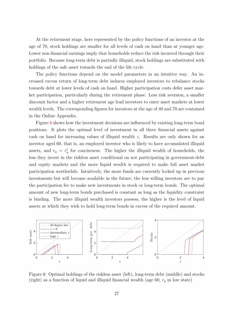
Figure 6 shows how the investment decisions are influenced by existing long-term bond

positions. It plots the optimal level of investment in all three financial assets against

cash on hand for increasing values of illiquid wealth z. Results are only shown for an

investor aged 60, that is, an employed investor who is likely to have accumulated illiquid

assets, and rq = rlq for conciseness. The higher the illiquid wealth of households, the

less they invest in the riskless asset conditional on not participating in government-debt

and equity markets and the more liquid wealth is required to make full asset market

participation worthwhile. Intuitively, the more funds are currently locked up in previous

investments but will become available in the future, the less willing investors are to pay

the participation fee to make new investments in stock or long-term bonds. The optimal

amount of new long-term bonds purchased is constant as long as the liquidity constraint

is binding. The more illiquid wealth investors possess, the higher is the level of liquid

assets at which they wish to hold long-term bonds in excess of the required amount.

0 2 40

2

4

0 2 40

2

4

0 2 40

2

4

Figure 6: Optimal holdings of the riskless asset (left), long-term debt (middle) and stocks(right) as a function of liquid and illiquid financial wealth (age 60, rq in low state)

27

4 Simulations

This section reports results from simulations of the baseline model outlined above and an

application to the period of historically low US Treasury returns between 2009 and 2013.

4.1 Baseline Results

I simulate the model for T = 80 − 26 = 54 years, for I individuals with idiosyncratic

shocks Ui,t, Ni,tTt=1 and for J aggregate shock sequences rs,t, rq,tTt=1. I and J are cho-

sen sufficiently large to guarantee full convergence of all model moments presented below.

Households have an initial endowment of liquid financial assets amounting to 50% of the

permanent component of labour income and half of the households additionally have illiq-

uid initial wealth at the value of 25% of permanent labour income, which is approximately

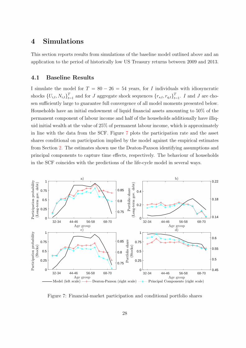
in line with the data from the SCF. Figure 7 plots the participation rate and the asset

shares conditional on participation implied by the model against the empirical estimates

from Section 2. The estimates shown use the Deaton-Paxson identifying assumptions and

principal components to capture time effects, respectively. The behaviour of households

in the SCF coincides with the predictions of the life-cycle model in several ways.

32-34 44-46 56-58 68-700

0.25

0.5

0.75

1

0.75

0.8

0.85

32-34 44-46 56-58 68-700

0.2

0.4

0.14

0.18

0.22

32-34 44-46 56-58 68-700

0.25

0.5

0.75

1

0.75

0.8

0.85

32-34 44-46 56-58 68-700

0.25

0.5

0.75

1

0.45

0.5

0.55

0.6

Figure 7: Financial-market participation and conditional portfolio shares

28

The dynamics of asset market participation in the model mirror the patterns of par-

ticipation in the markets for equity and long-term debt estimated from the SCF data.

Participation in financial markets is low at first in the model, since initial wealth and

hence desired savings are too low for it to be profitable to pay the participation cost and

then increases sharply as agents accumulate wealth. The participation rate first flattens

and then peaks at the age of 59-61. It declines again as agents retire and fall back to

wealth levels at which paying the participation cost to invest in the two risky assets ceases

to be beneficial.

The panels b) and d) show the average simulated conditional asset shares together

with the corresponding empirical estimates. The conditional long-term government debt

share in the model increases between the ages of 35-37 and 62-64 and then declines. A

comparable pattern is visible but less-well pronounced in the data. The long-term debt

share equally increases between 32-34 and 41-43 as well as between 44-46 and 53-55 but

at a smaller scale and the estimated peak occurs at a slightly younger age. Because

cash on hand on average increases with age during the employment stage, households

rebalance their portfolios from stocks towards long-term bonds to reduce the risk they

are facing through their financial portfolio in the model. Accordingly, the model predicts

a declining conditional stock share over the course of the working life which is confirmed

by the SCF data. When agents retire, non-financial income falls which implies that they

wish to decrease the risk of their financial investments. The fact that agents also save less

partially offsets this effect. On aggregate the stock share continues to decline. The lack of

liquidity of long-term debt makes it increasingly less attractive as a replacement for stock

holdings during the retirement phase. Since both the stock share and the long-term debt

share fall, the share of the residual category increases. The empirical estimates suggest

that the same is true in the US data.

While the stylised facts about the life-cycle dynamics of asset market participation,

the conditional stock share and the conditional long-term debt share uncovered in Section

2 can be rationalised using the model, the predicted dynamics are more muted in the

SCF estimates compared to the model. This may suggest that a standard life-cycle model

somewhat overstates the responsiveness of US households to life-cycle influences but may

equally be a result of noise in the survey data or the fact that a part of the asset holdings

have to be imputed. The investment decisions of the model agents are crucially driven by

wealth accumulation. Therefore it is instructive to investigate the evolution of wealth in

more detail to further gauge the congruence of observed household decisions with optimal

model behaviour.

29

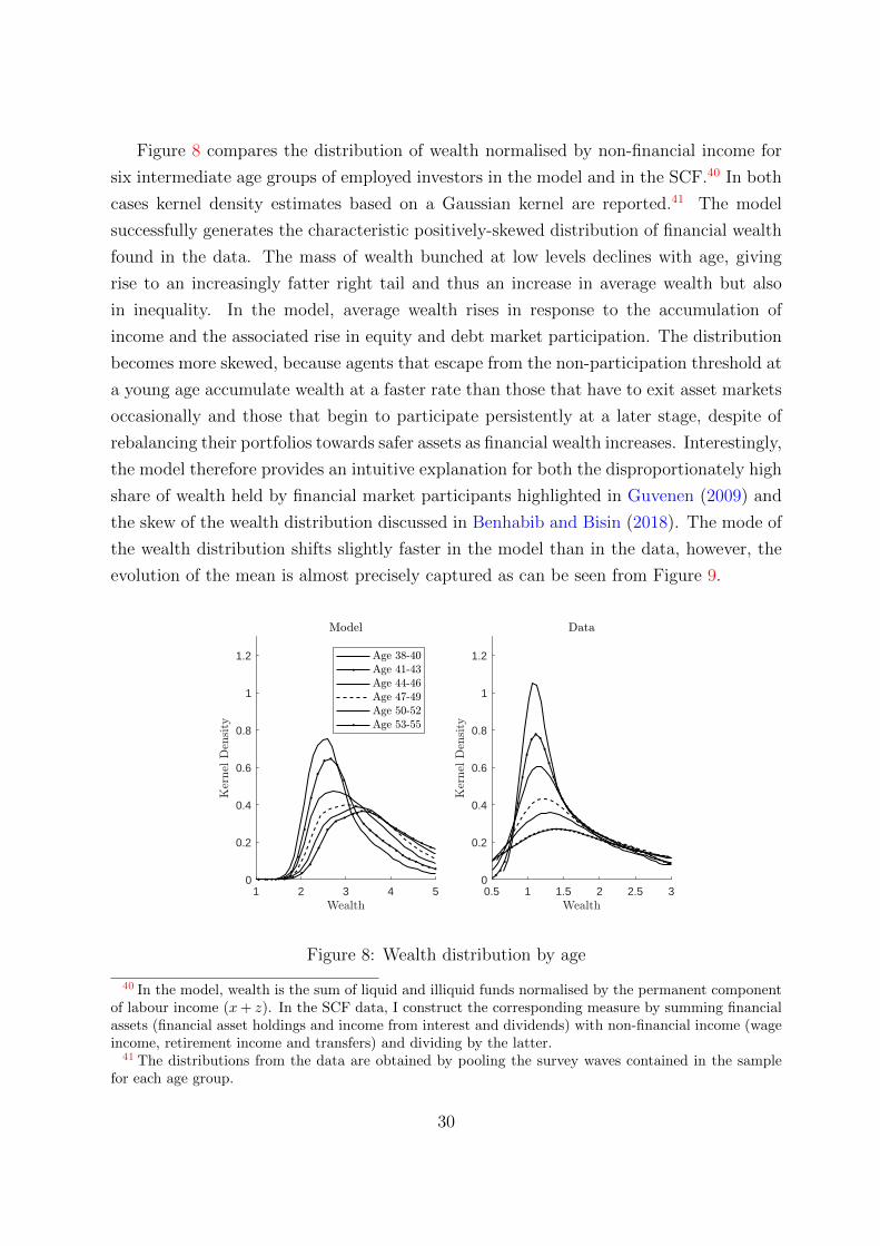
Figure 8 compares the distribution of wealth normalised by non-financial income for

six intermediate age groups of employed investors in the model and in the SCF.40 In both

cases kernel density estimates based on a Gaussian kernel are reported.41 The model

successfully generates the characteristic positively-skewed distribution of financial wealth

found in the data. The mass of wealth bunched at low levels declines with age, giving

rise to an increasingly fatter right tail and thus an increase in average wealth but also

in inequality. In the model, average wealth rises in response to the accumulation of

income and the associated rise in equity and debt market participation. The distribution

becomes more skewed, because agents that escape from the non-participation threshold at

a young age accumulate wealth at a faster rate than those that have to exit asset markets

occasionally and those that begin to participate persistently at a later stage, despite of

rebalancing their portfolios towards safer assets as financial wealth increases. Interestingly,

the model therefore provides an intuitive explanation for both the disproportionately high

share of wealth held by financial market participants highlighted in Guvenen (2009) and

the skew of the wealth distribution discussed in Benhabib and Bisin (2018). The mode of

the wealth distribution shifts slightly faster in the model than in the data, however, the

evolution of the mean is almost precisely captured as can be seen from Figure 9.

1 2 3 4 50

0.2

0.4

0.6

0.8

1

1.2

0.5 1 1.5 2 2.5 30

0.2

0.4

0.6

0.8

1

1.2

Figure 8: Wealth distribution by age

40 In the model, wealth is the sum of liquid and illiquid funds normalised by the permanent componentof labour income (x+ z). In the SCF data, I construct the corresponding measure by summing financialassets (financial asset holdings and income from interest and dividends) with non-financial income (wageincome, retirement income and transfers) and dividing by the latter.

41 The distributions from the data are obtained by pooling the survey waves contained in the samplefor each age group.

30

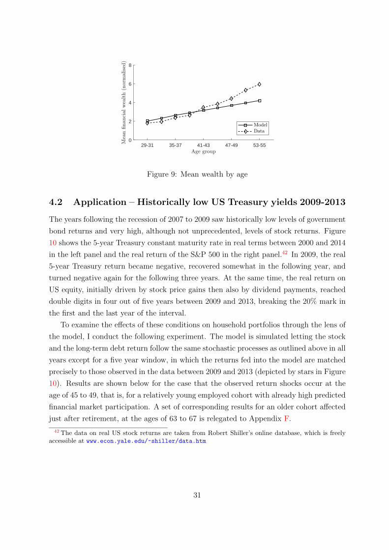
29-31 35-37 41-43 47-49 53-550

2

4

6

8

Figure 9: Mean wealth by age

4.2 Application – Historically low US Treasury yields 2009-2013

The years following the recession of 2007 to 2009 saw historically low levels of government

bond returns and very high, although not unprecedented, levels of stock returns. Figure

10 shows the 5-year Treasury constant maturity rate in real terms between 2000 and 2014

in the left panel and the real return of the S&P 500 in the right panel.42 In 2009, the real

5-year Treasury return became negative, recovered somewhat in the following year, and

turned negative again for the following three years. At the same time, the real return on

US equity, initially driven by stock price gains then also by dividend payments, reached

double digits in four out of five years between 2009 and 2013, breaking the 20% mark in

the first and the last year of the interval.

To examine the effects of these conditions on household portfolios through the lens of

the model, I conduct the following experiment. The model is simulated letting the stock

and the long-term debt return follow the same stochastic processes as outlined above in all

years except for a five year window, in which the returns fed into the model are matched

precisely to those observed in the data between 2009 and 2013 (depicted by stars in Figure

10). Results are shown below for the case that the observed return shocks occur at the

age of 45 to 49, that is, for a relatively young employed cohort with already high predicted

financial market participation. A set of corresponding results for an older cohort affected

just after retirement, at the ages of 63 to 67 is relegated to Appendix F.

42 The data on real US stock returns are taken from Robert Shiller’s online database, which is freelyaccessible at www.econ.yale.edu/~shiller/data.htm

31

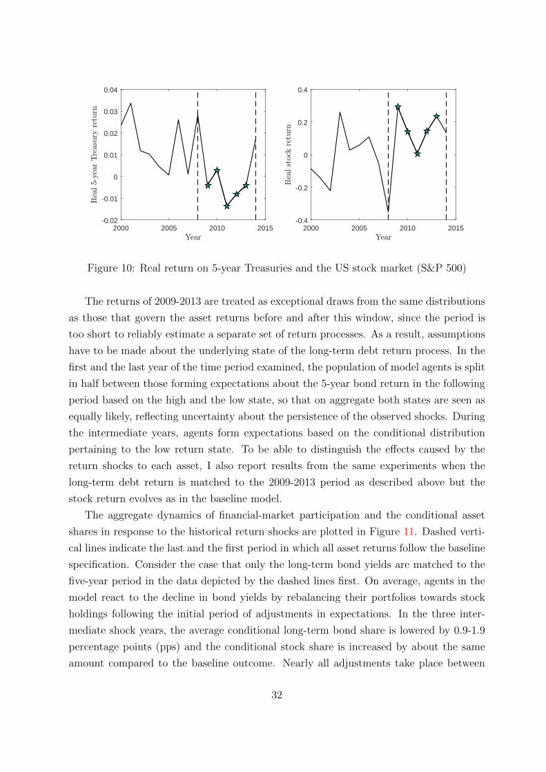
2000 2005 2010 2015Year

-0.02

-0.01

0

0.01

0.02

0.03

0.04Rea

l5-

year

Tre

asury

retu

rn

2000 2005 2010 2015Year

-0.4

-0.2

0

0.2

0.4

Rea

lst

ock

retu

rn

Figure 10: Real return on 5-year Treasuries and the US stock market (S&P 500)

The returns of 2009-2013 are treated as exceptional draws from the same distributions

as those that govern the asset returns before and after this window, since the period is

too short to reliably estimate a separate set of return processes. As a result, assumptions

have to be made about the underlying state of the long-term debt return process. In the

first and the last year of the time period examined, the population of model agents is split

in half between those forming expectations about the 5-year bond return in the following

period based on the high and the low state, so that on aggregate both states are seen as

equally likely, reflecting uncertainty about the persistence of the observed shocks. During

the intermediate years, agents form expectations based on the conditional distribution

pertaining to the low return state. To be able to distinguish the effects caused by the

return shocks to each asset, I also report results from the same experiments when the

long-term debt return is matched to the 2009-2013 period as described above but the

stock return evolves as in the baseline model.

The aggregate dynamics of financial-market participation and the conditional asset

shares in response to the historical return shocks are plotted in Figure 11. Dashed verti-

cal lines indicate the last and the first period in which all asset returns follow the baseline

specification. Consider the case that only the long-term bond yields are matched to the

five-year period in the data depicted by the dashed lines first. On average, agents in the

model react to the decline in bond yields by rebalancing their portfolios towards stock

holdings following the initial period of adjustments in expectations. In the three inter-

mediate shock years, the average conditional long-term bond share is lowered by 0.9-1.9

percentage points (pps) and the conditional stock share is increased by about the same

amount compared to the baseline outcome. Nearly all adjustments take place between

32

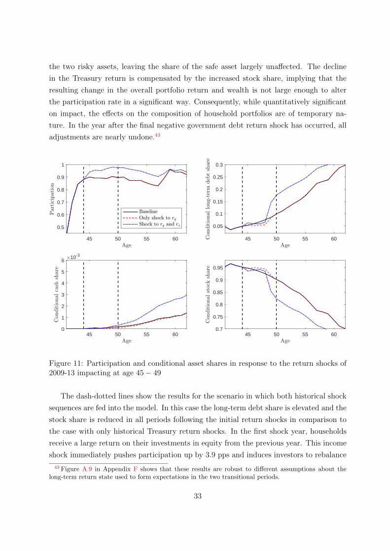
the two risky assets, leaving the share of the safe asset largely unaffected. The decline

in the Treasury return is compensated by the increased stock share, implying that the

resulting change in the overall portfolio return and wealth is not large enough to alter

the participation rate in a significant way. Consequently, while quantitatively significant

on impact, the effects on the composition of household portfolios are of temporary na-

ture. In the year after the final negative government debt return shock has occurred, all

adjustments are nearly undone.43

45 50 55 60

0.5

0.6

0.7

0.8

0.9

1

45 50 55 60

0.05

0.1

0.15

0.2

0.25

0.3

45 50 55 600

1

2

3

4

5

610-3

45 50 55 600.7

0.75

0.8

0.85

0.9

0.95

Figure 11: Participation and conditional asset shares in response to the return shocks of2009-13 impacting at age 45− 49

The dash-dotted lines show the results for the scenario in which both historical shock

sequences are fed into the model. In this case the long-term debt share is elevated and the

stock share is reduced in all periods following the initial return shocks in comparison to

the case with only historical Treasury return shocks. In the first shock year, households

receive a large return on their investments in equity from the previous year. This income

shock immediately pushes participation up by 3.9 pps and induces investors to rebalance

43 Figure A.9 in Appendix F shows that these results are robust to different assumptions about thelong-term return state used to form expectations in the two transitional periods.

33

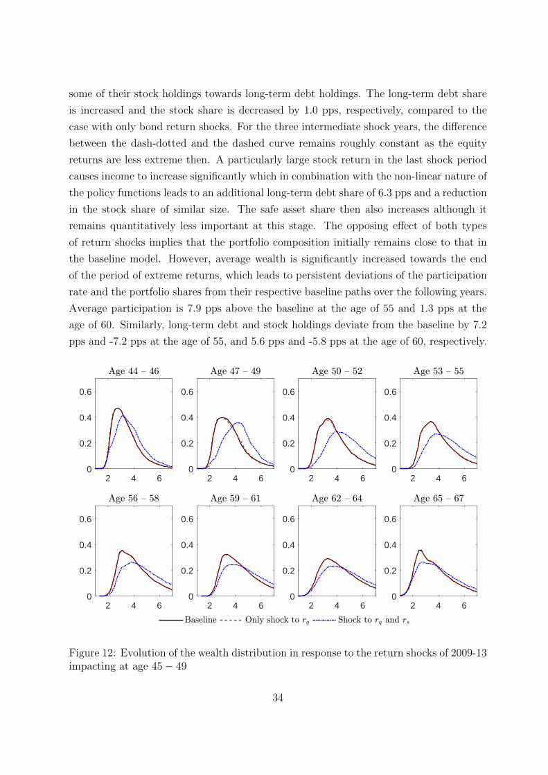
some of their stock holdings towards long-term debt holdings. The long-term debt share

is increased and the stock share is decreased by 1.0 pps, respectively, compared to the

case with only bond return shocks. For the three intermediate shock years, the difference

between the dash-dotted and the dashed curve remains roughly constant as the equity

returns are less extreme then. A particularly large stock return in the last shock period

causes income to increase significantly which in combination with the non-linear nature of

the policy functions leads to an additional long-term debt share of 6.3 pps and a reduction

in the stock share of similar size. The safe asset share then also increases although it

remains quantitatively less important at this stage. The opposing effect of both types

of return shocks implies that the portfolio composition initially remains close to that in

the baseline model. However, average wealth is significantly increased towards the end

of the period of extreme returns, which leads to persistent deviations of the participation

rate and the portfolio shares from their respective baseline paths over the following years.

Average participation is 7.9 pps above the baseline at the age of 55 and 1.3 pps at the

age of 60. Similarly, long-term debt and stock holdings deviate from the baseline by 7.2

pps and -7.2 pps at the age of 55, and 5.6 pps and -5.8 pps at the age of 60, respectively.

2 4 60

0.2

0.4

0.6

2 4 60

0.2

0.4

0.6

2 4 60

0.2

0.4

0.6

2 4 60

0.2

0.4

0.6

2 4 60

0.2

0.4

0.6

2 4 60

0.2

0.4

0.6

2 4 60

0.2

0.4

0.6

2 4 60

0.2

0.4

0.6

Figure 12: Evolution of the wealth distribution in response to the return shocks of 2009-13impacting at age 45− 49

34

Figure A.10 in the Appendix contains an analogous set of results for households that

are confronted with the historical sequence of return shocks at the age of 63 to 67. During

the retirement phase, households rebalance their portfolios towards the more liquid safe

asset rather than long-term debt. In this case, the stock return shocks therefore lead to

a more persistent increase in the stock share.

The historical return shocks have a significant effect on the distribution of wealth

in the model. Figure 12 shows the predicted evolution of the wealth distribution among

employed investors affected at the age of 45 to 49 as above. The shocks to the stock return

raise average wealth by increasing the mass in the right tail of the distribution. Investors

that are able to afford significant stock holdings when the shocks first hit experience a

large increase in their wealth levels, while the others are “left behind”. Deviations from

the baseline still exist when agents retire, suggesting that booms in the stock market lead

to persistent increases in inequality. For generations that experience the shocks at an

older age, the wealth distribution is strongly affected during the retirement stage, as can

be seen from Figure A.11.

5 Conclusion

Households systematically rebalance their financial portfolios as they accumulate wealth.

Nearly riskless assets like cash or bank deposits, long-term bonds like Treasury notes or

Treasury bonds, and equity play distinctive roles in this process. At low levels of liquid

wealth, the expected benefits from participating in the markets for long-term debt and

equity do not outweigh the costs, implying that households save through low-cost assets

with a low return. As they accumulate more cash on hand and save more, entering the

stock market becomes profitable. Cash holdings due to a pure savings motive markedly

decline at this point. At levels of liquid wealth just above the participation threshold,

investment income is small compared to labour income. Agents can therefore afford to

invest a large share of their financial portfolio in equity without being exposed to an

excessive amount of risk on aggregate. The additional accumulation of liquid wealth

implies that investment income as a fraction of total income increases. As a result, the

average asset-market participant reduces the equity share and increases the share of safer

assets to limit their risk exposure. My model suggests that long-term debt rather than

cash is used by households to readjust the risk properties of their portfolios in this way.

In accordance with debt instruments like US savings bonds, which can be cashed by

households only at a significant cost in the first five years after they have been issued,

35

government debt is assumed to be partially illiquid in the model. Consequently, the

portfolio-choice problem of households in a given period is dependent on past investments

in long-term debt. The higher the illiquid wealth of a household before retirement, the

less it invests in the riskless asset conditional on not acquiring new government debt

and stocks, the more liquid wealth is required for full asset-market participation to be

beneficial and the higher the level of cash on hand at which new government bonds are

purchased.

The micro-level behaviour in the model gives rise to aggregate dynamics that are in

line with data from the SCF. The asset-market participation rate is inverse U-shaped, the

average stock share monotonically decreases and the average long-term government-bond

share mildly increases until the age of 62 to 64 and then declines. The wealth distribution

is increasingly skewed to the right, because households that begin to invest in equity

consistently at a young age accumulate wealth faster than those that join later and those

that are forced to exit temporarily.

Cocco (2004) investigates the role that investment in housing plays for household port-

folios. He shows that for a fixed participation cost the rate of equity market participation

and, at a young age in particular, the equity share, are lower if model agents are permitted

to invest in housing. The interactions of housing with long-term debt investments and

their implications for equity holdings are left for future work.

A model-based decomposition of the effects resulting from the fluctuations in asset

returns observed in the US between 2009 and 2013 shows that the observed decline in long-

term bond yields has sizeable effects on the composition of household portfolios. Since

the average participation rate and wealth remain nearly unaffected, these effects are of

temporary nature. The observed stock-return shocks give households an additional motive

to rebalance their portfolios in the short-run, lead the asset-market participation rate to

increase and shift additional mass into the right tail of the wealth distribution, which

leads to persistent changes in the conditional asset shares. Naturally, the decomposition

used here is hypothetical. An important question relevant, for example, for evaluating the

macroeconomic effects of large-scale purchases of long-term bonds by central banks is to

what degree lowered bond yields exert upward pressure on stock prices. In the presence of

a strong link between the two, the model suggests that unconventional monetary policy in

the form of government debt purchases raises average consumption but causes inequality

to increase for several decades.

36

A Asset Categorisation

This section shows how the set of financial assets sampled in the SCF is divided into the

three broad categories stocks, long-term government debt and residual assets. I begin by

discussing selected assignments. The categorisation of all assets is shown in Table A.1.

Savings bonds and tax-exempt bonds are issued by the Department of the Treasury

and municipal, county or state governments, respectively. They typically have a maturity

of at least five years and are therefore treated as long-term government debt.

US government (agency) debt contains Bills, Notes and Bonds. As explained in the

text, Bills are classified as short-term and Notes/Bonds as long-term. According to the

“Monthly Statement of the Public Debt of the United States” from December 2007, 22.1%

of total marketable debt held by the public were Bills and the remainder Notes/Bonds.

Households are assumed to hold long-term and short-term debt at this proportion.

Certificates of deposit are a fixed-term savings product issued by banks, credit unions

and thrift institutions; they are allocated to the residual category.

Government bond investment funds are allocated in the same way as direct holdings

of US government debt.

Hybrid investment funds are allocated equally to stocks and government debt. Gov-

ernment debt is again split into long-term and short-term debt as described above.

Individual Retirement Accounts (IRAs) and Keogh Plans can include a variety of dif-

ferent financial assets. The Employee Benefit Research Institute (EBRI) estimates that,

in 2008, a total of 45.8% of funds in IRAs were held in the form of equity (38.5% in

equity mutual funds, directly held individual stocks, and other 100%-equity investment

vehicles; they add to this 60% of balanced, lifestyle/lifecycle, target-date funds, and any

other funds that have a partial investment in equities and bonds, which make up 12.1%

of all funds in IRAs).44 I assign 18.4% to long-term government debt (the remaining 40%

of hybrid equity-bond funds and all bond investments). Money and other assets make up

35.8% and are classified as “residual” for the purposes of this paper. Keogh Plans are

similar to IRAs but designed for self-employed individuals. I assume that funds held in

Keogh Plans are invested as in IRAs.

Life insurance and annuities are assigned to the residual category, since life insurances

and annuities are claims to a safe future payoff (stream).

Other managed assets include trusts and managed investment accounts which are

counted towards stocks here.

44 See “IRA Asset Allocation and Characteristics of the CDHP Population, 2005-2010”, May 2011,available at www.ebri.org/publications/notes.

37

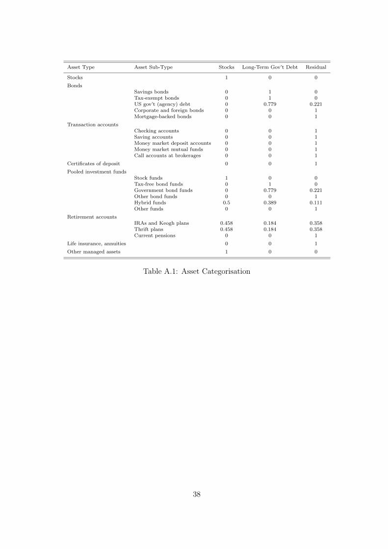
Asset Type Asset Sub-Type Stocks Long-Term Gov’t Debt Residual

Stocks 1 0 0

BondsSavings bonds 0 1 0Tax-exempt bonds 0 1 0US gov’t (agency) debt 0 0.779 0.221Corporate and foreign bonds 0 0 1Mortgage-backed bonds 0 0 1

Transaction accountsChecking accounts 0 0 1Saving accounts 0 0 1Money market deposit accounts 0 0 1Money market mutual funds 0 0 1Call accounts at brokerages 0 0 1

Certificates of deposit 0 0 1

Pooled investment fundsStock funds 1 0 0Tax-free bond funds 0 1 0Government bond funds 0 0.779 0.221Other bond funds 0 0 1Hybrid funds 0.5 0.389 0.111Other funds 0 0 1

Retirement accountsIRAs and Keogh plans 0.458 0.184 0.358Thrift plans 0.458 0.184 0.358Current pensions 0 0 1

Life insurance, annuities 0 0 1

Other managed assets 1 0 0

Table A.1: Asset Categorisation

38

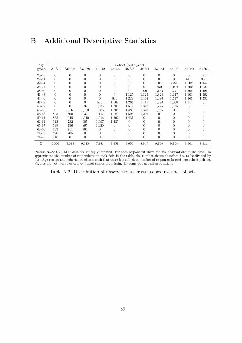
B Additional Descriptive Statistics

Age Cohort (birth year)group ’31-’33 ’34-’36 ’37-’39 ’40-’42 ’43-’45 ’46-’48 ’49-’51 ’52-’54 ’55-’57 ’58-’60 ’61-’63

26-28 0 0 0 0 0 0 0 0 0 0 49529-31 0 0 0 0 0 0 0 0 0 510 85832-34 0 0 0 0 0 0 0 0 822 1,009 1,04735-37 0 0 0 0 0 0 0 850 1,102 1,200 1,12338-40 0 0 0 0 0 0 906 1,155 1,227 1,305 1,29641-43 0 0 0 0 0 1,125 1,125 1,328 1,447 1,601 1,36244-46 0 0 0 0 890 1,229 1,462 1,386 1,517 1,365 1,23047-49 0 0 0 810 1,162 1,265 1,411 1,690 1,608 1,511 050-52 0 0 834 1,035 1,286 1,519 1,327 1,725 1,535 0 053-55 0 916 1,000 1,086 1,206 1,480 1,321 1,566 0 0 056-58 825 800 937 1,117 1,180 1,595 1,295 0 0 0 059-61 855 945 1,010 1,016 1,292 1,437 0 0 0 0 062-64 943 782 905 1,097 1,235 0 0 0 0 0 065-67 739 756 867 1,020 0 0 0 0 0 0 068-70 733 711 760 0 0 0 0 0 0 0 071-73 690 705 0 0 0 0 0 0 0 0 074-76 518 0 0 0 0 0 0 0 0 0 0

Σ 5,303 5,615 6,313 7,181 8,251 9,650 8,847 9,700 9,258 8,501 7,411

Notes: N=86,030. SCF data are multiply imputed. For each respondent there are five observations in the data. Toapproximate the number of respondents in each field in the table, the number shown therefore has to be divided byfive. Age groups and cohorts are chosen such that there is a sufficient number of responses in each age-cohort pairing.Figures are not multiples of five if asset shares are missing for some but not all imputations.

Table A.2: Distribution of observations across age groups and cohorts

39

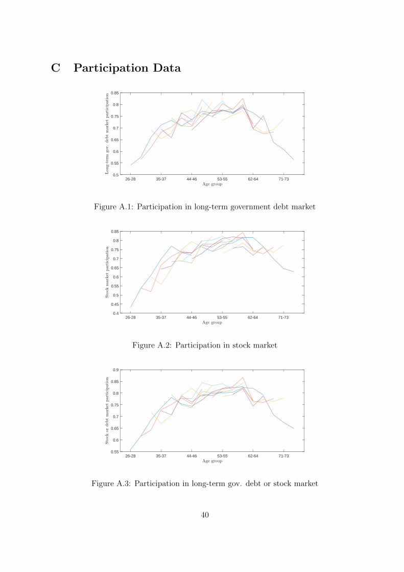
C Participation Data

26-28 35-37 44-46 53-55 62-64 71-730.5

0.55

0.6

0.65

0.7

0.75

0.8

0.85

Figure A.1: Participation in long-term government debt market

26-28 35-37 44-46 53-55 62-64 71-730.4

0.45

0.5

0.55

0.6

0.65

0.7

0.75

0.8

0.85

Figure A.2: Participation in stock market

26-28 35-37 44-46 53-55 62-64 71-730.55

0.6

0.65

0.7

0.75

0.8

0.85

0.9

Figure A.3: Participation in long-term gov. debt or stock market

40

D Estimation

The controls included in the estimations are binary variables indicating the marital status,

education, race, type of employment as well as information on household debt and pension

plans. The exclusion restrictions imposed in the estimations are discussed below.

In the model of the stock share, the assumption maintained is that, at low levels of

education, a marginal amount of additional schooling increases the likelihood of stock

market participation but not the portfolio share conditional on participation. Compared

to some years of high-school attendance, a completed high-school education may provide

individuals with knowledge about investment opportunities and lower the costs of access

to the stock market, but should have no direct effect on the stock share conditional on

participation when other characteristics such as the occupation of the individual are con-

trolled for. In the Probit selection equation, having earned a high-school diploma and

visited college for some time without graduating has a significant effect on the participa-

tion probability (at the 1% level) and is insignificant in a regression of the second-step

residuals on the explanatory variables (at the 5% level).

Without an exclusion restriction, multicollinearity issues arise if the inverse Mills ratio

(IMR) is close to being linear in the linear predictions of the Probit equation. Figure A.4

which plots the IMR against the linear predictions shows that this is not a concern here.

Figure A.5 depicts the predicted stock share for the case that the exclusion restriction

is imposed and the case that it is not imposed and the identification relies on functional

form assumptions. Deaton-Paxson restrictions are used to address the age-period-cohort

problem. The estimates are almost identical despite of the fact that the excluded vari-

ables are strongly significant in the selection equation. Excluding the variables in the

outcome equation has a small ‘direct’ effect resulting in an insignificant parallel shift of

the estimated age profile. However, the shape of the estimated age profile is unaffected

by the exclusion restriction. Following the view in the literature that the Heckman sam-

ple selection model is the correct model to separate stock market participation from the

conditional portfolio share, see e.g. Fagereng et al. (2017), we can therefore be confident

that the age dynamics of the conditional stock share are captured accurately.

41

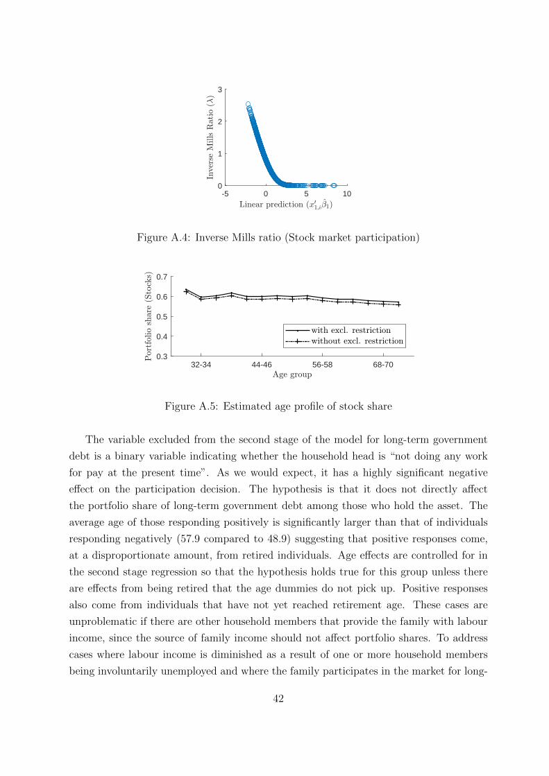
-5 0 5 100

1

2

3

Figure A.4: Inverse Mills ratio (Stock market participation)

32-34 44-46 56-58 68-700.3

0.4

0.5

0.6

0.7

Figure A.5: Estimated age profile of stock share

The variable excluded from the second stage of the model for long-term government

debt is a binary variable indicating whether the household head is “not doing any work

for pay at the present time”. As we would expect, it has a highly significant negative

effect on the participation decision. The hypothesis is that it does not directly affect

the portfolio share of long-term government debt among those who hold the asset. The

average age of those responding positively is significantly larger than that of individuals

responding negatively (57.9 compared to 48.9) suggesting that positive responses come,

at a disproportionate amount, from retired individuals. Age effects are controlled for in

the second stage regression so that the hypothesis holds true for this group unless there

are effects from being retired that the age dummies do not pick up. Positive responses

also come from individuals that have not yet reached retirement age. These cases are

unproblematic if there are other household members that provide the family with labour

income, since the source of family income should not affect portfolio shares. To address

cases where labour income is diminished as a result of one or more household members

being involuntarily unemployed and where the family participates in the market for long-

42

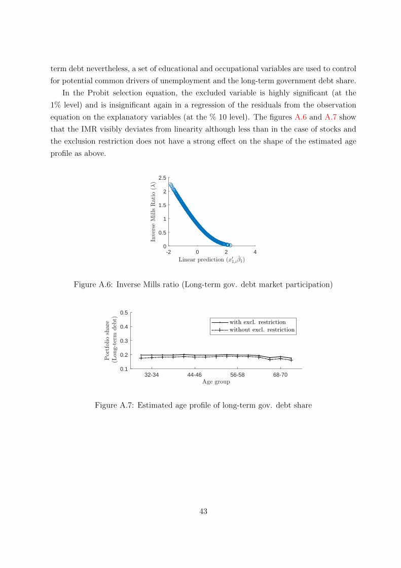
term debt nevertheless, a set of educational and occupational variables are used to control

for potential common drivers of unemployment and the long-term government debt share.

In the Probit selection equation, the excluded variable is highly significant (at the

1% level) and is insignificant again in a regression of the residuals from the observation

equation on the explanatory variables (at the % 10 level). The figures A.6 and A.7 show

that the IMR visibly deviates from linearity although less than in the case of stocks and

the exclusion restriction does not have a strong effect on the shape of the estimated age

profile as above.

-2 0 2 40

0.5

1

1.5

2

2.5

Figure A.6: Inverse Mills ratio (Long-term gov. debt market participation)

32-34 44-46 56-58 68-700.1

0.2

0.3

0.4

0.5

Figure A.7: Estimated age profile of long-term gov. debt share

43

OLS(1) (2)

Long-term debt -0.6381***

Cash -0.7542***

Wealth 0.0006*** -0.0001**

(in millions)

min(Nimp) 4,299 4,299Total N 21,531 21,531

Sign. tests

Time Eff’s 4.4*** 5.9***

(d.o.f.) (6) (6)

Notes: Dependent variable: Stock share. Data aremultiply imputed. For each respondent, there are fiveobservations in the data. Point estimates are aver-ages over five separate estimations. Strd. errors areadjusted in an appropriate way (∗p<0.1, ∗∗p<0.05,∗∗∗p<0.01). Nimp is number of obs. for imputationimp ∈ 1, 2, ..., 5. For joint significant tests, avrg.F-test stat. shown, degrees of freedom in parentheses.

Table A.3: Conditional correla-tions of long-term debt and cashshare with stock share

44

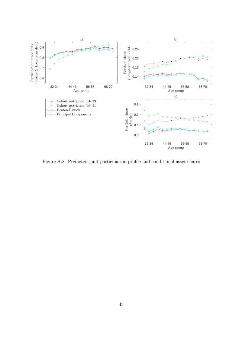
32-34 44-46 56-58 68-70

0.6

0.7

0.8

0.9

32-34 44-46 56-58 68-70

0.14

0.18

0.22

0.26

32-34 44-46 56-58 68-70

0.5

0.6

0.7

0.8

Figure A.8: Predicted joint participation profile and conditional asset shares

45

E Normalisation

Consider the amount of funds brought into the period first. Cash on hand of an employed

investor can be normalised as follows

X = rsS−1 + rbB−1 + δ−1rqQ−1 + Y (26)

X

P= rs

S−1P−1

P−1P+ rb

B−1P−1

P−1P+ δ−1rq

Q−1P−1

P−1P+PU

P(27)

x =rss−1 + rbb−1 + δ−1rqq−1

GN+ U (28)

and illiquid assets as

z =(1− δ−1)rqq−1

GN(29)

For a retired investor, one obtains

X = rsS−1 + rbB−1 + δ−1rqQ−1 + Ω (30)

X

PTret= rs

S−1

PTret+ rb

B−1

PTret+ δ−1rq

Q−1

PTret+ωPTretPTret

(31)

x = rss−1 + rbb−1 + δ−1rqq−1 + ω (32)

and

z = (1− δ−1)rqq−1 (33)

The budget constraint of a financial-market participant and a non-participant then be-

come, respectively,

c+ s(1 + ψs) + b+ q + ψ = x+ z (34)

c+ b+ q = x+ z (35)

Indirect utility can be transformed in a similar way. Starting with an employed par-

ticipant, we have

vp (X,Z, rq, P, t) = maxC,S,B,Q

u(C) + βEU ′,P ′,r′s,r′q |P,rqv

(X ′, Z ′, r′q, P

′, t+ 1)

(36)

vp (X,Z, rq, P, t)

P 1−γ = maxC,S,B,Q

u(C)

P 1−γ + βEU ′,P ′,r′s,r′q |P,rq

v(X ′, Z ′, r′q, P

′, t+ 1)

P 1−γ (37)

vp

(X

P,Z

P, rq, 1, t

)= max

C,S,B,Qu

(C

P

)+ βEU ′,P ′,r′s,r

′q |P,rqv

(X ′

P,Z ′

P, r′q,

P ′

P, t+ 1

)(38)

46

vp (x, z, rq, t) = maxc,s,b,q

u (c) + βEU ′,P ′,r′s,r′q |P,rqv

(x′P ′

P, z′P ′

P, r′q,

P ′

P, t+ 1

)(39)

vp (x, z, rq, t) = maxc,s,b,q

u (c) + βEU ′,N ′,r′s,r′q |rq(GN

′)1−γv(x′, z′, r′q, t+ 1

)(40)

Indirect utility of an employed non-participant is

vn (x, z, rq, t) = maxc,b

u (c) + βEU ′,N ′,r′q |rq(GN′)1−γv

(x′, z′, r′q, t+ 1

)(41)

and

v (x, z, rq, t) = max vp (x, z, rq, t) , vn (x, z, rq, t) (42)

The corresponding equations for a retired investor are

vp (x, z, rq, t) = maxc,s,b,q

u (c) + βEr′s,r′q |rqv

(x′, z′, r′q, t+ 1

)(43)

vn (x, z, rq, t) = maxc,b

u (c) + βEr′q |rqv(x′, z′, r′q, t+ 1

)(44)

47

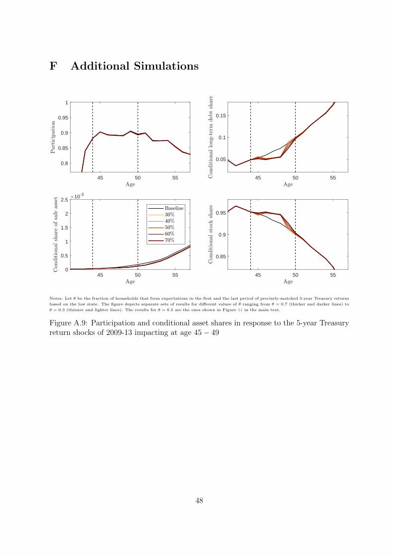
F Additional Simulations

45 50 55

0.8

0.85

0.9

0.95

1

45 50 55

0.05

0.1

0.15

45 50 550

0.5

1

1.5

2

2.510-3

45 50 55

0.85

0.9

0.95

Notes: Let θ be the fraction of households that form expectations in the first and the last period of precisely-matched 5-year Treasury returns

based on the low state. The figure depicts separate sets of results for different values of θ ranging from θ = 0.7 (thicker and darker lines) to

θ = 0.3 (thinner and lighter lines). The results for θ = 0.5 are the ones shown in Figure 11 in the main text.

Figure A.9: Participation and conditional asset shares in response to the 5-year Treasuryreturn shocks of 2009-13 impacting at age 45− 49

48

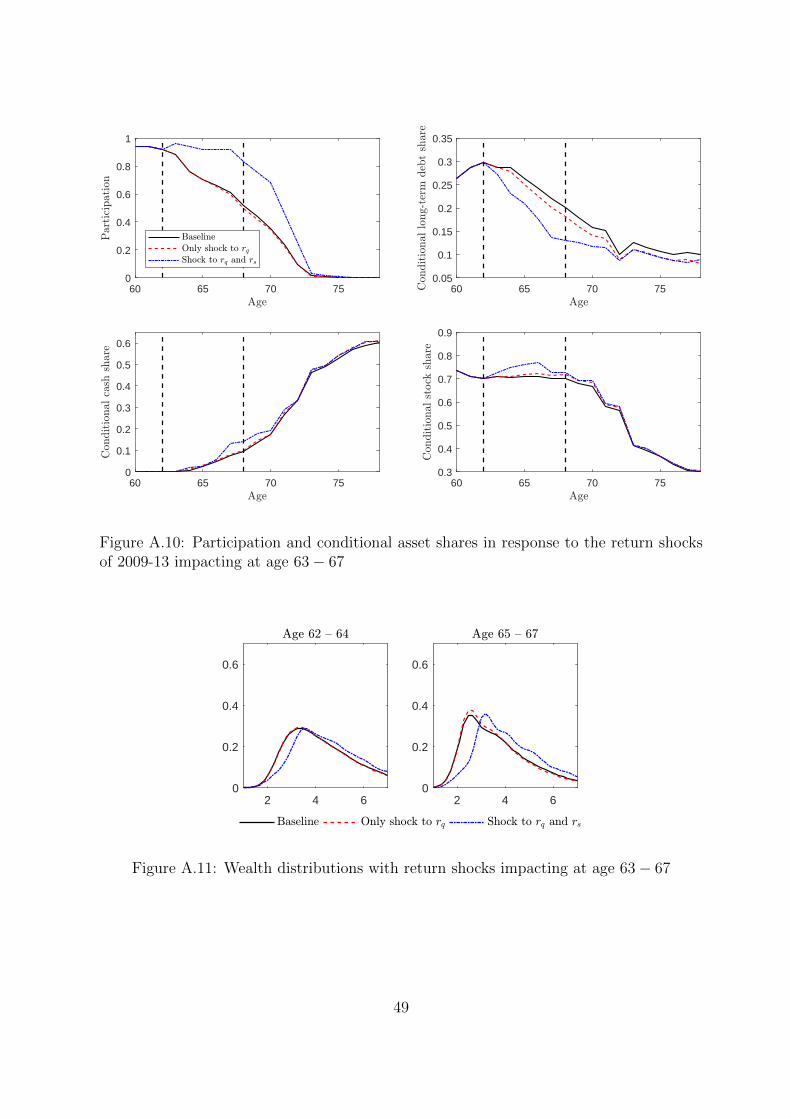
60 65 70 750

0.2

0.4

0.6

0.8

1

60 65 70 750.05

0.1

0.15

0.2

0.25

0.3

0.35

60 65 70 750

0.1

0.2

0.3

0.4

0.5

0.6

60 65 70 750.3

0.4

0.5

0.6

0.7

0.8

0.9

Figure A.10: Participation and conditional asset shares in response to the return shocksof 2009-13 impacting at age 63− 67

2 4 60

0.2

0.4

0.6

2 4 60

0.2

0.4

0.6

Figure A.11: Wealth distributions with return shocks impacting at age 63− 67

49

References

Alan, S. (2006). Entry costs and stock market participation over the life cycle. Review of

Economic Dynamics, 9:588–611.

Ameriks, J. and Zeldes, S. P. (2004). How Do Household Portfolio Shares Vary With

Age? Columbia University mimeo.

Bagliano, F. C., Fugazza, C., and Nicodano, G. (2014). Optimal Life-Cycle Portfolios for

Heterogeneous Workers. Review of Finance, 18(6):2283–2323.

Benhabib, J. and Bisin, A. (2018). Skewed Wealth Distributions: Theory and Empirics.

Journal of Economic Literature, 56(4):1261–1291.

Bonaparte, Y., Cooper, R., and Zhu, G. (2012). Consumption smoothing and portfolio

rebalancing: The effects of adjustment costs. Journal of Monetary Economics, 59:751–

768.

Browning, M., Crawford, I., and Knoef, M. (2012). The age-period cohort problem: set

identification and point identification. CeMMAP working paper CWP02/12, Centre for

Microdata Methods and Practice, Institute for Fiscal Studies.

Cagetti, M. (2003). Wealth accumulation over the life cycle and precautionary savings.

Journal of Business and Economic Statistics, 21(3):339–353.

Campanale, C., Fugazza, C., and Gomes, F. (2015). Life-cycle portfolio choice with liquid

and illiquid financial assets. Journal of Monetary Economics, 71:67–83.

Campbell, J. Y. and Viceira, L. M. (2001). Who Should Buy Long-Term Bonds. The

American Economic Review, 91(1):99–127.

Carroll, C. D., Hall, R. E., and Zeldes, S. P. (1992). The Buffer-Stock Theory of Saving:

Some Macroeconomic Evidence. Brookings Papers on Economic Activity, 23(2):61–156.

Cocco, J. F. (2004). Portfolio Choice in the Presence of Housing. The Review of Financial

Studies, 18(2):535–567.

Cocco, J. F., Gomes, F. J., and Maenhout, P. J. (2005). Consumption and Portfolio

Choice of the Life Cycle. The Review of Financial Studies, 18(2):491–533.

Deaton, A. (1997). The Analysis of Household Surveys - A Microeconomic Approach to

Development Policy. The Johns Hopkins University Press, Baltimore, MD.

50

Deaton, A. and Paxson, C. (1994). Saving, Growth, and Aging in Taiwan. In Studies in

the Economics of Aging, NBER Chapters, pages 331–362. National Bureau of Economic

Research, Inc.

Fagereng, A., Gottlieb, C., and Guiso, L. (2017). Asset Market Participation and Portfolio

Choice over the Life-Cycle. The Journal of Finance, 72(2):705–750.

Gomes, F. and Michaelides, A. (2005). Optimal Life-Cycle Asset Allocation: Understand-

ing the Empirical Evidence. The Journal of Finance, 60(2):869–904.

Guiso, L., Haliassos, M., and Jappelli, T. (2003). Stockholding in Europe: Where Do We

Stand and Where Do We Go? Economic Policy, 18(36):123 – 170.

Guvenen, F. (2009). A Parsimonious Macroeconomic Model for Asset Pricing. Econo-

metrica, 77(6):1711–1750.

Haliassos, M. (2008). Household Portfolios. In Durlauf, S. N. and Blume, L. E., editors,

The New Palgrave Dictionary of Economics, pages 331 – 362. Palgrave Macmillan.

Haliassos, M. and Michaelides, A. (2003). Portfolio Choice and Liquidity Constraints.

International Economic Review, 44(1):143–177.

Hussey, R. and Tauchen, G. (1991). Quadrature-Based Methods for Obtaining Approxi-

mate Solutions to Nonlinear Asset Pricing Models. Econometrica, 59(2):371–396.

Kennickell, A. B. (2008). The role of over-sampling of the wealthy in the survey of

consumer finances. In IFC Bulletin No 28, IFC’s contribution to the 56th ISI Session,

Lisbon, 2007, pages 403–408. Bank for International Settlements.

Merton, R. C. (1969). Lifetime Portfolio Selection under Uncertainty: The Continuous-

Time Case. The Review of Economics and Statistics, 51(3):247–257.

Merton, R. C. (1971). Optimum Consumption and Portfolio Rules in a Continuous-Time

Model. Journal of Economic Theory, 3:373–413.

Munnell, A. H. and Soto, M. (2005). What Replacement Rates Do Households Actually

Experience in Retirement? Working Paper 2005-10, Center for Retirement Research at

Boston College.

Ryder, N. B. (1965). The Cohort as a Concept in the Study of Social Change. American

Sociological Review, 30(6):843–861.

51

Samuelson, P. A. (1969). Lifetime Portfolio Selection By Dynamic Stochastic Program-

ming. The Review of Economics and Statistics, 51(3):239–246.

Viceira, L. M. (2001). Optimal Portfolio Choice for Long-Horizon Investors with Non-

tradable Labor Income. The Journal of Finance, 56(2):433–470.

Wachter, J. A. (2003). Risk aversion and allocation to long-term bonds. Journal of

Economic Theory, 112:325–333.

Woodford, M. (2001). Fiscal requirements for price stability. Journal of Money, Credit

and Banking, 33:669–728.

52