Long-Term Monitoring and Analysis of a Curved Concrete Box

91

International Journal of Concrete Structures and Materials

Vol.2, No.2, pp. 91~98, December 2008

Long-Term Monitoring and Analysis of a Curved Concrete

Box-Girder Bridge

Sungchil Lee,1)

Maria Q. Feng,2)

Seok-Hee Hong,3)

and Young-Soo Chung4)

(Received October 6, 2008, Revised November 30, 2008, Accepted November 30, 2008)

Abstract : Curved bridges are important components of a highway transportation network for connecting local roads and

highways, but very few data have been collected in terms of their field performance. This paper presents two-years monitoring and

system identification results of a curved concrete box-girder bridge, the West St. On-Ramp, under ambient traffic excitations. The

authors permanently installed accelerometers on the bridge from the beginning of the bridge life. From the ambient vibration data

sets collected over the two years, the element stiffness correction factors for the columns, the girder, and boundary springs were

identified using the back-propagation neural network. The results showed that the element stiffness values were nearly 10%

different from the initial design values. It was also observed that the traffic conditions heavily influence the dynamic characteristics

of this curved bridge. Furthermore, a probability distribution model of the element stiffness was established for long-term

monitoring and analysis of the bridge stiffness change.

Keywords : long-term monitoring, curved concrete bridge, back-propagation neural network, probability distribution model, acceleration mea-

surement, traffic excitation, modal frequency, element stiffness

1. Introduction

Recent advances in sensor, communication, and computer tech-

nologies have made automated monitoring of bridge structures a

promising alternative to the traditional visual inspection. In fact,

many researchers have studied sensor-based monitoring of bridges,

most of which dealt with long-span bridges.1-3

As for medium-

and short-span bridges, studies have focused on straight bridges,

but not curved ones. 4,5

Medium- and short-span curved bridges are inevitable in a

modern highway system to connect local roadways to highways in

interchanges. It is important to monitor and study the performance

of such bridges. Different from long-span bridges whose ambient

vibrations are caused by both wind and traffic excitations, medium-

and short-span bridges are mainly excited by traffic loads.

Many system identification methods have been proposed for

identifying structural dynamic properties based on ambient vibra-

tion tests, but they suffer from errors caused by unknown input

forces. In reality, different input energy level to excite a bridge

results in different dynamic properties, i.e. natural frequency,

mode shape, damping ratio. The authors experienced on the WSO

that the natural frequencies of the bridge from a braking test and a

bumping test were not the same because of the different exciting

energy level.6

Therefore it is important to use ambient vibration

data sets under a similar traffic condition when identifying the

structural dynamic properties. Since not only the excitation energy

level but also the dynamic interactions between traveling vehicles

and the bridge, but also the environmental conditions such as the

temperature and humidity affect the dynamic properties of bridges, a

probability distribution model established by long-term bridge

monitoring would provide more information about the change of

the bridge structural parameter (such as the stiffness) rather than

one point estimation at a specific time during a whole bridge life.

The neural network-based system identification method 7-10

has

several advantages compared with conventional system identifica-

tion methods. It is more capable of indentifying elemental stiffness

values based on the partially and incompletely measured mode

parameters due to the limited sensor number. Furthermore, it is

convenient to use neural networks to parameterize any properties

of the structures, such as the effective shear area, as the unknowns

to be identified. In contrast to many other system identification

methods in which the sensitivity matrix may become unstable espe-

cially for complex structural systems, the neural network approach

does not require calculation of the sensitivity matrix, and thus can

be applied to complex civil engineering structures with less numeri-

cal difficulty.

In this paper, the back-propagation neural network was adopted

to identify the element stiffness of the WSO using the traffic-

induced ambient vibration data selected from the population of

1)KCI Member, Dept. of Civil & Env. Engineering, University of

California Irvine, Irvine, 92697 USA. E-mail: [email protected])University of California Irvine, Dept. of Civil & Env. Engineer-

ing, Irvine, 92697 USA. 3)KCI Member, Naekyung Engineering Co., LTD. Anyang 431-060,

Korea.4)KCI Member, Dept. of Civil Engineering, Chung-Ang University,

Ansung 456-756, Korea.

Copyright ⓒ 2008, Korea Concrete Institute. All rights reserved,

including the making of copies without the written permission of

the copyright proprietors.

92│International Journal of Concrete Structures and Materials (Vol.2 No.2, December 2008)

data sets collected during the two years of monitoring. The proba-

bility distribution model of the element stiffness was established to

account for the uncertainties from environmental conditions.

2. Instrumentation and monitoring system

Collaborating with the California Department of Transportation

(Caltrans), the authors installed sensors on a new curved concrete

bridge, the West Street On-Ramp (WSO), on Interstate 5 in Ana-

heim, California, during its construction.6 The bridge opened to

traffic in 2001. As shown in Figs. 1 and 2, this three-span continu-

ous bridge has a single-cell cast-in-place pre-stressed post-tension

box girder. The total length of the bridge is 151.33 m with the span

lengths of 45.77 m, 60.12 m, and 45.44 m. The radius of curvature

is 165.00 m. The bridge is supported by two columns and sliding

bearings on both abutments. The sliding bearings allow creep,

shrinkage, and thermal expansion or contraction.

The monitoring system installed at the WSO includes 11 force-

balance servo-type accelerometers mounted permanently at selected

locations on the concrete surface, 10 strain gauges embedded in

the concrete, one longitudinal displacement sensor and soil pres-

sure sensor at the abutment. The locations and measurement direc-

tions of the accelerometers are shown in Fig. 3, and one of the

accelerometers is shown in a photo in Fig. 4. The accelerometers

on the superstructure were placed along the centerline of the

girder.

The strain sensors were embedded in concrete members of the

bridge to measure dynamic strains. Each strain sensor was welded

to a dummy reinforcing bar and embedded in concrete during the

construction. Figure 5 shows the locations of the strain sensors.

The displacement sensor was placed to measure the relative dis-

placement between abutment 1 and the box girder in the longitudi-

nal direction and the soil pressure sensor was embedded in the

back of abutment 1.

3. Finite element model of WSO

For the purpose of identifying the bridge structural parameters,

particularly the stiffness, from the measured dynamic responses to

traffic excitations, a 3-dimensional finite element (FE) model of

the WSO was developed using the OpenSees program.11

The

bridge was modeled by beam elements, with 200 elements for the

deck and 16 elements for each column. The boundary conditions

of the finite element model were assumed as fixed for the columns

and as springs for the bearings at both of the abutments. The bear-

ing stiffness values were assigned according to the design guide-

lines,12

as 9.7 × 105

kN/m, 18.8 × 105

kN/m, and 21.6 × 105

kN/m

respectively for the longitudinal, transverse and vertical directions.

The rotational spring stiffness values were assigned as 7.5 × 107

kN-m/rad and 4.7 × 10

7kN.m/rad respectively along the longitudinal

and vertical axes in the horizontal plane. Table 1 summarizes the

Young’s modulus and the moment of inertia of the column and thedeck from the design drawings and Fig. 6 shows the FE model of

the WSO.

4. Back-propagation neural network

A back-propagation neural network was developed for identify-

ing the element stiffness of the WSO from the measured dynamic

response to traffic excitations. The input of the network are natural

frequencies extracted from the measured acceleration responses,

while the output of the network are the element stiffness correction

factors which are defined as ratios of the identified stiffness and

the baseline stiffness. The neural network was trained through

finite element analysis.

4.1 Architecture of neural networkAs shown in the architecture in Fig. 7, the back-propagation

neural network consists of two hidden layers, as well as the input

and output layers. Each hidden layer has 10 nodes i.e. neurons.

Tangent sigmoid and pure linear functions were used as the trans-

Fig. 1 Typical section of WSO.

Fig. 2 View of WSO.

Fig. 3 Installation of accelerometer.

International Journal of Concrete Structures and Materials (Vol.2 No.2, December 2008)│93

fer function for hidden layers and the output layer, respectively.

Even though the neural network approach can produce stable

results for system identification, cautions should be exercised in

selecting the input parameters. First of all, the input parameters

should be obtained easily and accurately from experiments. Sec-

ondly, the input parameters must be sensitive to the output targets.

Though the input parameters to the neural network could be any

dynamic characteristics of a structure such as mode shapes, mode

frequencies, and/or modal damping, the first three mode frequen-

cies were chosen as the input parameters in this study because of

the limited number of the installed accelerometers at the bridge and

insufficient information regarding the other dynamic properties.

As output parameters, the element stiffness correction factors

for the girder, columns, and boundary springs of the WSO were

selected. Considering the young age of the bridge, it is assumed

that the girder is experiencing a uniform stiffness change along

entire girder and so as to each of the columns and abutment soil.

In other words, the output of the neural network consists of one

stiffness correction factor for the girder, one stiffness correction

factor for the column, and one stiffness correction factor of the soil

springs at the bridge abutment.

Fig. 4 Layout of accelerometers.

Fig. 5 Layout of strain sensors.

Table 1 Moment of inertia of column and deck element (m4).

ElementMoment of Inertia Young’s Modulus

(MN/m2)Iy Iz

Column 2.780 2.780 29,575

Deck 5.472 48.532 26,658

Fig. 6 Finite element model of WSO.

Fig. 7 Architecture of artificial neural network.


4.2 Neural network training process Training patterns for the neural network were generated through

finite element analysis of the bridge using the OpenSees program.

For the generation of the training patterns, the correction factors

were varied from 0.7 to 1.0 for both the girder and the columns

and from 0.5 to 1.0 for the abutment boundary springs. Because of

the high uncertainty of the boundary condition, the correction fac-

tor of the boundary spring was assumed broader than those of the

columns and the girder. For each set of the given correction fac-

tors, the corresponding modal frequencies of the bridge model

were computed. Table 2 shows examples of the training patterns.

In total 4805 training sets were generated. The back-propagation

neural network was trained using the Matlab toolbox.14

To avoid

the overfitting problem, an early stopping method was employed.

The neural network performance was tested for 30 cases and the

results were satisfactory with error of less than 5%.

4.3 Selection of ambient vibration dataAs mentioned earlier, the energy level of the traffic excitations

affect the dynamic characteristics of a bridge structure. This is

demonstrated by an example in Fig. 8, in which power spectral den-

sity functions obtained by applying the frequency domain decom-

position method13

from the measured acceleration responses of

the WSO. Figures 8 (a) and (b) are based on two different sets of

measurement data under different traffic excitation conditions. In

Fig. 8 (a) two clear peaks appear around 2.4 Hz and 3.6 Hz and

other frequencies between two peaks are suppressed. In Fig. 8 (b),

however, the frequencies between 2.5 Hz and 3.5 Hz are predomi-

nant. The different frequency characteristics shown in Figs. 8(a)

and (b) might have been caused by vehicle-bridge interactions, as

well as the different energy levels of the traffic excitations. Obvi-

ously using the extracted mode frequencies as the input to the neu-

ral network will result in different output results - stiffness correction

factors. Therefore, it is important to use the bridge dynamic responses

to similar traffic excitations for the purpose of long-term monitor-

ing and identification of the stiffness change. In this study, 20

ambient vibration data sets whose frequency contents are similar

to those from the preliminary finite element analysis were selected

from the 91 ambient vibration data collected in the two-year moni-

toring period. By doing so, the bridge response data sets heavily

affected by the vehicle-bridge dynamic interactions were avoided.

5. System identification results and probability distribution model

The first three modal natural frequencies of the WSO were

extracted from the 20 selected ambient vibration data sets using

the frequency decomposition method. Then by inputting into the

neural network these modal frequencies, the element stiffness cor-

rection factors of the bridge were identified.

5.1 Element stiffness correction factor Table 3 shows the identified element stiffness correction factors

over the period of two years. Figure 9 shows the dispersion of the

modal frequencies and the element stiffness correction factors.

The average values of the element stiffness correction factors are

0.911, 0.903, and 1.107 for the column, the girder, and the bound-

ary soil spring, respectively.

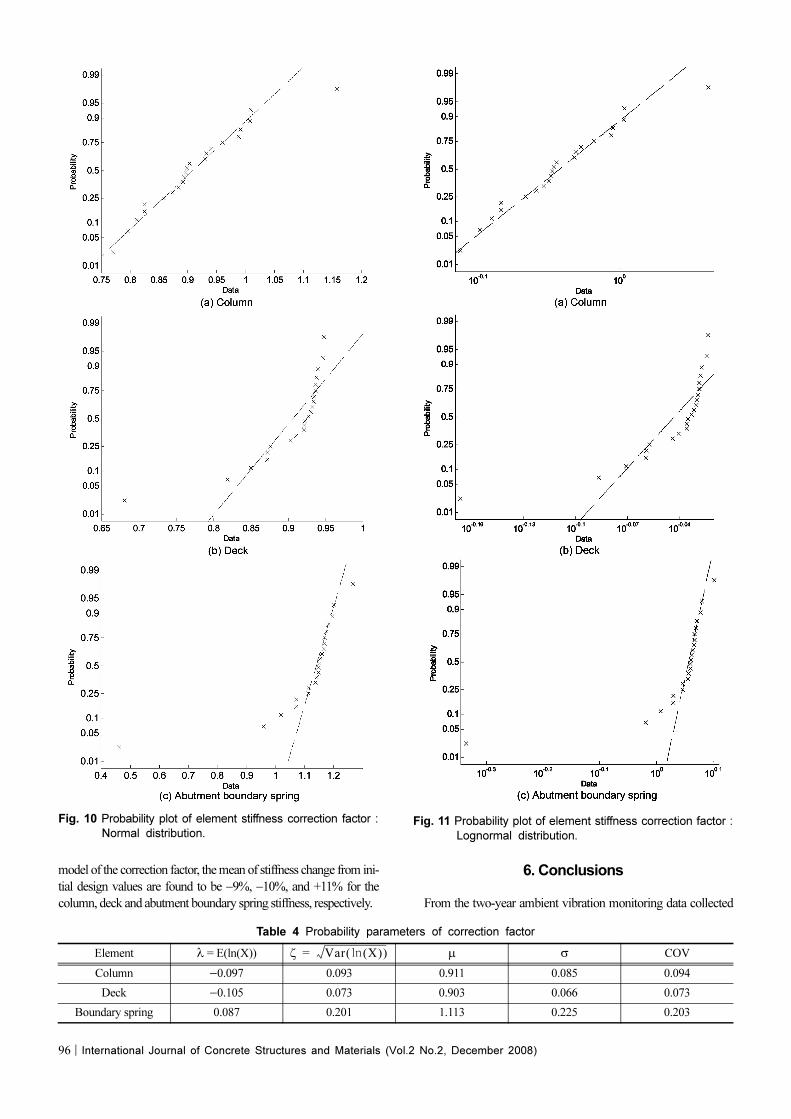
5.2 Probability distribution model of element stiffnessBased on the identified element stiffness from neural network,

the probability distribution models for the element stiffness correc-

tion factors were established. Figures 10 and 11 show the proba-

bility plots of the element stiffness correction factors assuming the

normal (Eq.1) and the log-normal distributions (Eq.2), respec-

tively.

(1)

(2)

fX

x( ) 1

σ 2π--------------

1

2---

x µ–

σ------------⎝ ⎠⎛ ⎞ 2

–exp= ∞– x ∞< <

fX

x( ) 1

2πζx-----------------

1

2---

xln λ–

ζ-----------------⎝ ⎠⎛ ⎞ 2

–exp= 0 x≤ ∞<

Table 2 Training patterns for the WSO.

NoInput (frequency in Hz) Output (correction factor)

1st mode 2

nd mode 3

rd mode Ccol Cdeck Cbnd

1 1.751 2.086 2.357 0.700 0.700 0.500

2 1.762 2.128 2.381 0.700 0.700 0.600

... ... ... ... ... ... ...

4805 2.084 2.509 2.819 1.000 1.000 1.000

Fig. 8 Power spectral density function from ambient vibration

data of WSO.


where, X is a random variable, µ and σ are the mean and standard

deviation respectively, of the variate, λ and ζ are, respectively, the

mean and standard deviation of ln(x).

For each of the bridge components (i.e., the girder and the col-

umn), the normal and the log-normal probability plots show simi-

lar results. Since the correction factors cannot be negative values,

the log-normal distribution was chosen as the probability distribu-

tion model for the element stiffness correction factors.

From Fig. 11, it is observed that all the data fit well with the log-

normal distribution for the correction factor of the column, but

some data slightly deviate for the girder and boundary spring. Fig-

ure 12 shows the log-normal distribution fitting curve and the

identified stiffness correction factor of each component. The param-

eters of the log-normal distribution of each component were calcu-

lated from the maximum likelihood estimation and they are

shown in Table 4. The mean and standard deviation values of each

correction factor in Table 4 were derived by Eq. (3) and (4)

(3)

(4)

It can be observed from Table 4 that the factor of variance of the

boundary spring is much higher than those of the column and the

girder. It means that the modal frequencies of the bridge are more

sensitive to the stiffness of the boundary soil than the bridge col-

umns and the girder. From the log-normal probability distribution

µ λ1

2---ζ

2+⎝ ⎠

⎛ ⎞exp=

σ2

µ ζ2( ) 1–exp( )=

Table 3 Element stiffness correction factors from neural network.

DateInput (Hz) Correction factor

First Second Third Ccol Cdeck Cbnd

2004/ 01/30 1.99 2.42 2.79 0.897 0.946 1.150

2004/ 03/30 1.91 2.42 2.75 0.991 0.930 1.168

2004/ 10/21 1.99 2.38 2.77 0.825 0.937 1.112

2004/ 11/03 1.91 2.40 2.59 0.894 0.819 0.959

2004/ 12/16 1.97 2.40 2.71 0.825 0.938 1.070

2005/ 02/ 11 2.03 2.36 2.81 0.892 0.911 1.071

2005/ 03/ 17 1.99 2.41 2.83 1.009 0.850 1.202

2005/ 05/ 17 1.95 2.40 2.73 0.874 0.937 1.148

2005/ 08/ 02 1.93 2.38 2.73 0.903 0.921 1.160

2005/ 09/ 21 1.95 2.40 2.79 0.940 0.923 1.174

2005/ 09/ 23 1.90 2.35 2.72 0.932 0.876 1.180

2005/ 10/ 28 1.99 2.42 2.78 0.884 0.948 1.141

2005/ 11 /22 1.93 2.63 2.71 0.960 0.934 1.153

2005/ 12/ 23 1.97 2.35 2.75 0.796 0.927 1.114

2006/ 01/ 14 1.99 2.42 2.81 0.930 0.933 1.166

2006/ 02/ 03 1.95 2.38 2.77 0.899 0.921 1.168

2006/ 03/ 13 1.99 2.42 2.85 1.158 0.681 1.265

2006/ 03/ 24 1.97 2.42 2.83 1.008 0.873 1.195

2006/ 05/ 08 1.97 2.40 2.75 0.858 0.940 1.138

2006/ 06/ 08 1.97 2.36 2.71 0.771 0.935 1.018

2006/ 09/ 081)

1.90 2.31 2.68 0.812 0.872 1.148

2006/ 09/ 082)

2.01 2.36 2.66 0.988 0.904 0.462

Average 1.96 2.39 2.75 0.911 0.903 1.1071)

: Field test -braking test, 2)

: Field test - bumping test

Fig. 9 Input and output parameter of BPNN.


model of the correction factor, the mean of stiffness change from ini-

tial design values are found to be −9%, −10%, and +11% for the

column, deck and abutment boundary spring stiffness, respectively.

6. Conclusions

From the two-year ambient vibration monitoring data collected

Fig. 10 Probability plot of element stiffness correction factor :

Normal distribution.Fig. 11 Probability plot of element stiffness correction factor :

Lognormal distribution.

Table 4 Probability parameters of correction factor

Element λ = E(ln(X)) µ σ COV

Column −0.097 0.093 0.911 0.085 0.094

Deck −0.105 0.073 0.903 0.066 0.073

Boundary spring 0.087 0.201 1.113 0.225 0.203

ζ Var X( )ln( )=


at the West St. On-Ramp, the change in the stiffness of the col-

umns, the girder, and the boundary spring was identified using a

back-propagation neural network. For this curved bridge, it was

found that the natural frequencies of the bridge extracted from the

measured vibration data were heavily influenced by the vehicle-

bridge interactions as well as the energy level of the traffic excita-

tions. For this study, 20 vibration measurement data sets showing

similar frequency response patterns were selected from the total

90 data sets. These data sets were considered to be excited by sim-

ilar traffic conditions and not influenced by the vehicle-bridge

interactions.

From the identified element stiffness correction factors, the

probability distribution model of the element stiffness was estab-

lished for the two-year monitoring period under the assumption of

the log-normal distribution. The higher factor of variance of the

correction factor of the abutment boundary spring indicated that

the modal frequencies of the bridge are more sensitive to the abut-

ment soil springs than the bridge columns and girder. In addition,

it was found that the identified stiffness values of the columns and

the girder were approximately 10% different from the design val-

ues.

In the future, the authors will continue collecting and analyzing

traffic-induced vibration data from the curved West St. On-Ramp.

A long-term trend in the element stiffness change will be traced in

the probabilistic framework. In addition, dynamic interactions

between traveling vehicles and the bridge structure will be studied,

which is believed to play an important role in the dynamic

response of a curved bridge.

Acknowledgments

This study was supported by the NaeKyung Engineering Com-

pany and the Infra-Structures Assessment Research Center (ISARC)

funded by the Ministry of Land, Transport, and Maritime Affairs

(MLTM), Korea. The authors gratefully acknowledge this support.

References

1. Shahawy, M. A. and Arockiasamy, M., “Analytical and measured

strains in Sunshine Skyway Bridge II,” Journal of Bridge Engi-

neering, Vol. 1, No. 2, 1996, pp. 87~97.

2. Barrish, R. A. Jr., Grimmelsman, K. A., and Aktan, A. E.,

“Instrumented monitoring of the Commodore Barry Bride,” Pro-

ceedings of SPIE, No. 3995, 2000, pp. 112~122.

3. Abe, M., Fujino, Y., Yanagihara, M., and Sato, M., “Mon-

itoring of Hakucho Suspension Bridge by Ambient Vibration Mea-

surement,” Proceedings of SPIE, No.3995, 2000, pp. 237~244

4. Sartor, R. R., Culmo, M. P., and DeWolf, J. T., “Short-term

Strain Monitoring of Bridge Structures.” Journal of Bridge

Engineering, Vol. 4, No.3, 1999, pp. 157~164.

5. Choi, S., Park, S., Bolton, R., Stubbs, N., and Sikorsky, C.,

“Periodic Monitoring of Physical Property Changes in a Con-

crete Box Girder Bridges.” Journal of Sound and Vibration, Vol.

278, 2004, pp. 365~381.

6. Feng, M. Q. and Kim, D. K., Long-Term Structural Per-

formance Monitoring of Two Highway Bridges, Technical Report of

the California Department of Transportation, 2001.

7. Yun, C. B., Yi, J. H., and Bahng, E. Y., ‘‘Joint Damage

Assessment of Framed Structures Using a Neural Networks Tech-

nique.’’ Engineering Structures, Vol. 23, No. 5, 2001, pp. 425~435.

8. Masri S., F., Smyth, A. W., Chassiakos, A. G., Caughey, T.

K., and Hunter, N. F., ‘‘Application of Neural Networks for

Detection of Changes in Nonlinear Systems”. Journal of Engi-

neering Mechanics, Vol. 126, No. 7, 2000, pp. 666~676.

9. Feng, M. Q. and Bahng, E. Y., “Damage Assessment of

Jacketed RC Columns Using Vibration Tests,” Journal of Struc-

tural Engineering, Vol. 125, No. 3, 1999, pp. 265~271.

10. Feng, M. Q., Kim, D. K., Yi, J-H and Chen, Y., “Baseline

Fig. 12 Log-normal distribution fitting of correction factors.


Models for Bridge Performance Monitoring.” Journal of Engi-

neering Mechanics, Vol. 130, No. 5, 2004, pp. 562~569.

11. Pacific Earthquake Engineering Research Center, OpenSees,

Reference Manual, PECCR 2001.

12. Federal Highway Administration, Seismic Design of Bridges

Design Example No.6: Three-span Continuous CIP Concrete Box

Bridge, FHWA, 1996.

13. Brinker, R., Zhang, L., and Andersen, P., “Modal Iden-

tification of Output-only System Using Frequency Domain

Decomposition.” Smart Material and Structure, Vol. 10, No. 3,

2001, pp. 441~455.

14. The Mathworks Inc, Neural Network Toolbox, 2004.

Documents

Long-Term Monitoring and Analysis of a Curved Concrete Box