Embed Size (px)
Citation preview

Longitudinal AIDS Data Analysis
Problem: Lengthy follow-up times required to evaluateefficacy of a new treatment (e.g., survival time ofHIV-infected patients)
Chapter 8.1 Case Study: Analysis of AIDS Data – p. 1/22

Longitudinal AIDS Data Analysis
Problem: Lengthy follow-up times required to evaluateefficacy of a new treatment (e.g., survival time ofHIV-infected patients)
Solution(?): Select an easily-measured biologicalmarker, known to be predictive of the clinical outcome,as a surrogate endpoint. In AIDS research, typically useCD4 count (number of lymphocytes/mm3 blood).
BUT several studies have cast doubt on this approach...
Example: Anglo-French “Concorde” trial showedimmediate AZT produces consistently higher CD4counts than deferred, but survival patterns in twogroups were nearly identical.
Chapter 8.1 Case Study: Analysis of AIDS Data – p. 1/22

Our data: the ddI/ddC study467 persons randomized to didanosine (ddI) orzalcitabine (ddC)
Chapter 8.1 Case Study: Analysis of AIDS Data – p. 2/22

Our data: the ddI/ddC study467 persons randomized to didanosine (ddI) orzalcitabine (ddC)
HIV-infected patients with AIDS or two CD4 counts of300 or less, and who had failed or could not toleratezidovudine (AZT)
⇒ all are very ill
Chapter 8.1 Case Study: Analysis of AIDS Data – p. 2/22

Our data: the ddI/ddC study467 persons randomized to didanosine (ddI) orzalcitabine (ddC)
HIV-infected patients with AIDS or two CD4 counts of300 or less, and who had failed or could not toleratezidovudine (AZT)
⇒ all are very ill
CD4 counts recorded at baseline, 2, 6, 12, and 18months (some missing)
covariates: age, sex, baseline AIDS Dx, baselineKarnofsky score, etc.
outcome variables: clinical disease progression, death
Chapter 8.1 Case Study: Analysis of AIDS Data – p. 2/22

Goal and Subplot of ddI/ddC study
Goal: Analyze the association among CD4 count,survival time, drug group, and AIDS diagnosis at studyentry (an indicator of disease progression status). Makerecommendations for clinical practice and use of CD4as surrogate marker for death in end-stage patients.
Chapter 8.1 Case Study: Analysis of AIDS Data – p. 3/22

Goal and Subplot of ddI/ddC study
Goal: Analyze the association among CD4 count,survival time, drug group, and AIDS diagnosis at studyentry (an indicator of disease progression status). Makerecommendations for clinical practice and use of CD4as surrogate marker for death in end-stage patients.
Subplot: ddI granted preliminary license in USA basedprimarily on its ability to “boost” CD4 count at 2 months.ddC makers would like to show a similar boost and/orcomparable survival time (“equivalency trial").
Chapter 8.1 Case Study: Analysis of AIDS Data – p. 3/22

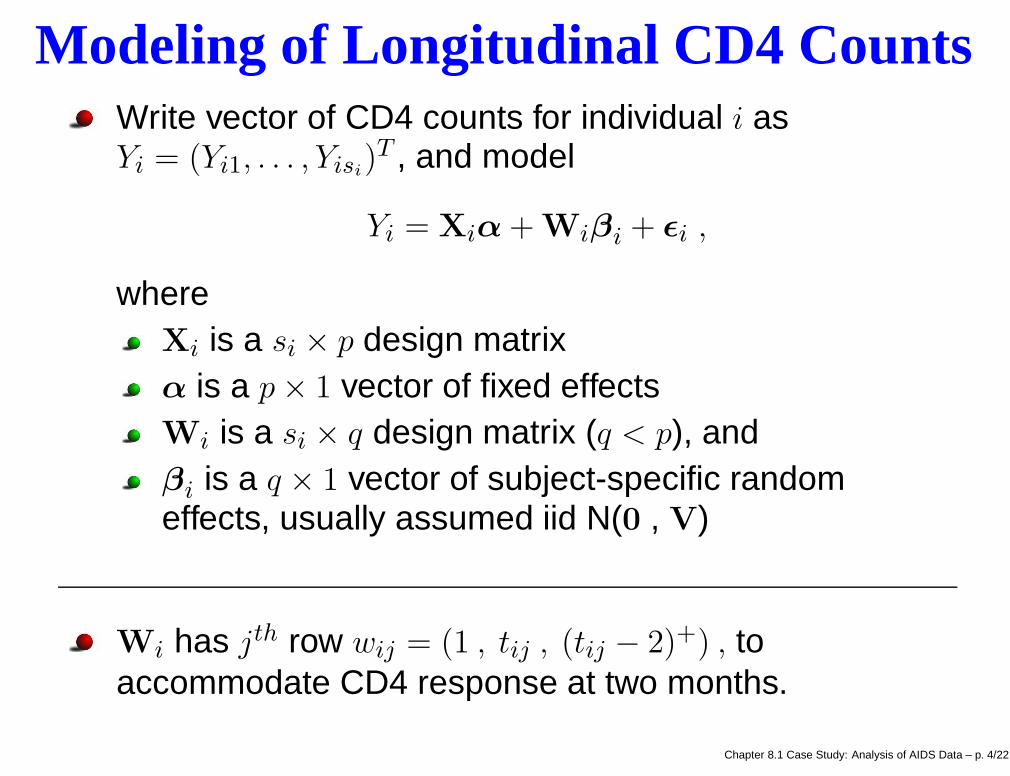
Modeling of Longitudinal CD4 CountsWrite vector of CD4 counts for individual i asYi = (Yi1, . . . , Yisi
)T , and model
Yi = Xiα + Wiβi + ǫi ,
where
Chapter 8.1 Case Study: Analysis of AIDS Data – p. 4/22

Modeling of Longitudinal CD4 CountsWrite vector of CD4 counts for individual i asYi = (Yi1, . . . , Yisi
)T , and model
Yi = Xiα + Wiβi + ǫi ,
whereXi is a si × p design matrix
Chapter 8.1 Case Study: Analysis of AIDS Data – p. 4/22

Modeling of Longitudinal CD4 CountsWrite vector of CD4 counts for individual i asYi = (Yi1, . . . , Yisi
)T , and model
Yi = Xiα + Wiβi + ǫi ,
whereXi is a si × p design matrixα is a p × 1 vector of fixed effects
Chapter 8.1 Case Study: Analysis of AIDS Data – p. 4/22

Modeling of Longitudinal CD4 CountsWrite vector of CD4 counts for individual i asYi = (Yi1, . . . , Yisi
)T , and model
Yi = Xiα + Wiβi + ǫi ,
whereXi is a si × p design matrixα is a p × 1 vector of fixed effectsWi is a si × q design matrix (q < p), and
Chapter 8.1 Case Study: Analysis of AIDS Data – p. 4/22

Modeling of Longitudinal CD4 CountsWrite vector of CD4 counts for individual i asYi = (Yi1, . . . , Yisi
)T , and model
Yi = Xiα + Wiβi + ǫi ,
whereXi is a si × p design matrixα is a p × 1 vector of fixed effectsWi is a si × q design matrix (q < p), andβi is a q × 1 vector of subject-specific randomeffects, usually assumed iid N(0 , V)
Chapter 8.1 Case Study: Analysis of AIDS Data – p. 4/22
Modeling of Longitudinal CD4 CountsWrite vector of CD4 counts for individual i asYi = (Yi1, . . . , Yisi
)T , and model
Yi = Xiα + Wiβi + ǫi ,
whereXi is a si × p design matrixα is a p × 1 vector of fixed effectsWi is a si × q design matrix (q < p), andβi is a q × 1 vector of subject-specific randomeffects, usually assumed iid N(0 , V)
Wi has jth row wij = (1 , tij , (tij − 2)+) , toaccommodate CD4 response at two months.
Chapter 8.1 Case Study: Analysis of AIDS Data – p. 4/22

Modeling of Longitudinal CD4 CountsWe account for the covariates by letting
Xi = (Wi | diWi | aiWi) , where
Chapter 8.1 Case Study: Analysis of AIDS Data – p. 5/22

Modeling of Longitudinal CD4 CountsWe account for the covariates by letting
Xi = (Wi | diWi | aiWi) , where
di = 1 if i received ddI; di = 0 if ddC
Chapter 8.1 Case Study: Analysis of AIDS Data – p. 5/22

Modeling of Longitudinal CD4 CountsWe account for the covariates by letting
Xi = (Wi | diWi | aiWi) , where
di = 1 if i received ddI; di = 0 if ddCai = 1 is i has an AIDS diagnosis at baseline; ai = 0if not
Chapter 8.1 Case Study: Analysis of AIDS Data – p. 5/22

Modeling of Longitudinal CD4 CountsWe account for the covariates by letting
Xi = (Wi | diWi | aiWi) , where
di = 1 if i received ddI; di = 0 if ddCai = 1 is i has an AIDS diagnosis at baseline; ai = 0if not
Likelihood:
n∏
i=1
Nsi(Yi|Xiα + Wiβi, σ
2Isi)
n∏
i=1
N3(βi|0,V) ,
Prior: N9(α|c,D) × IG(σ2|a, b) × IW (V|(ρR)−1, ρ)
⇒ easy full conditional distributions for Gibbs sampling!
Chapter 8.1 Case Study: Analysis of AIDS Data – p. 5/22

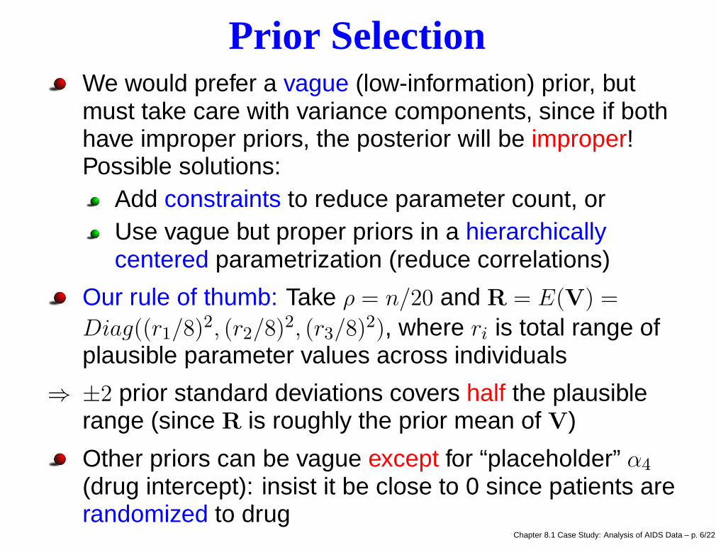
Prior SelectionWe would prefer a vague (low-information) prior, butmust take care with variance components, since if bothhave improper priors, the posterior will be improper!Possible solutions:
Chapter 8.1 Case Study: Analysis of AIDS Data – p. 6/22

Prior SelectionWe would prefer a vague (low-information) prior, butmust take care with variance components, since if bothhave improper priors, the posterior will be improper!Possible solutions:
Add constraints to reduce parameter count, or
Chapter 8.1 Case Study: Analysis of AIDS Data – p. 6/22

Prior SelectionWe would prefer a vague (low-information) prior, butmust take care with variance components, since if bothhave improper priors, the posterior will be improper!Possible solutions:
Add constraints to reduce parameter count, orUse vague but proper priors in a hierarchicallycentered parametrization (reduce correlations)
Our rule of thumb: Take ρ = n/20 and R = E(V) =
Diag((r1/8)2, (r2/8)2, (r3/8)2), where ri is total range ofplausible parameter values across individuals
⇒ ±2 prior standard deviations covers half the plausiblerange (since R is roughly the prior mean of V)
Chapter 8.1 Case Study: Analysis of AIDS Data – p. 6/22
Prior SelectionWe would prefer a vague (low-information) prior, butmust take care with variance components, since if bothhave improper priors, the posterior will be improper!Possible solutions:
Add constraints to reduce parameter count, orUse vague but proper priors in a hierarchicallycentered parametrization (reduce correlations)
Our rule of thumb: Take ρ = n/20 and R = E(V) =
Diag((r1/8)2, (r2/8)2, (r3/8)2), where ri is total range ofplausible parameter values across individuals
⇒ ±2 prior standard deviations covers half the plausiblerange (since R is roughly the prior mean of V)
Other priors can be vague except for “placeholder” α4
(drug intercept): insist it be close to 0 since patients arerandomized to drug
Chapter 8.1 Case Study: Analysis of AIDS Data – p. 6/22
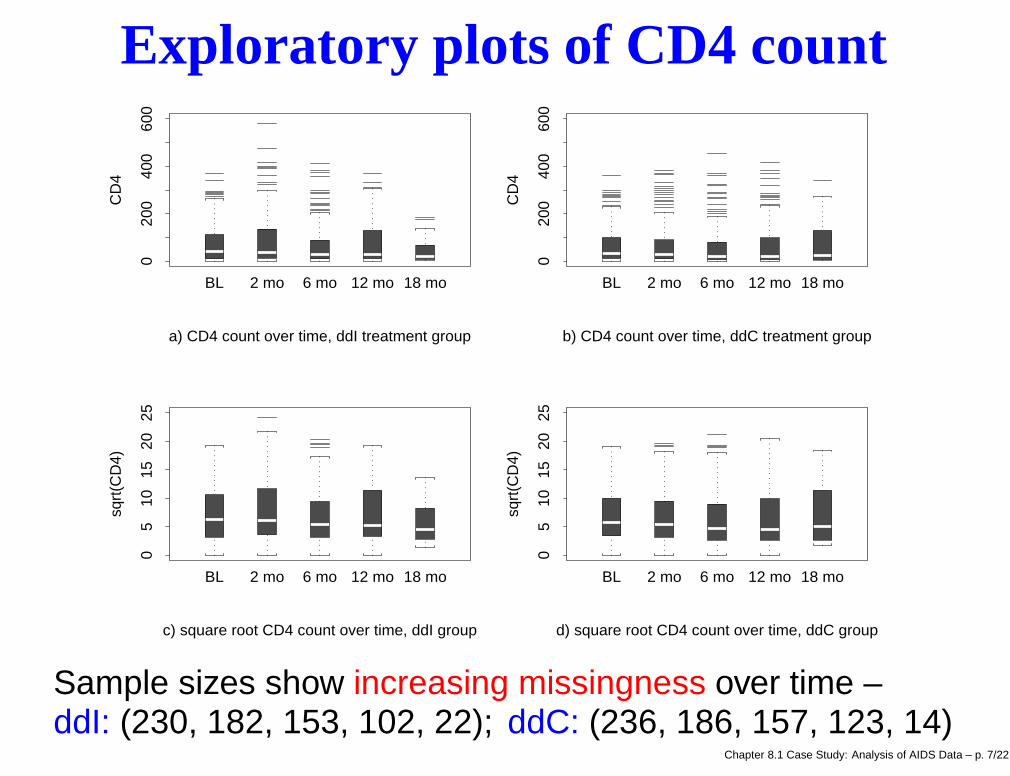
Exploratory plots of CD4 count
020
040
060
0
BL 2 mo 6 mo 12 mo 18 mo
CD
4
a) CD4 count over time, ddI treatment group
020
040
060
0
BL 2 mo 6 mo 12 mo 18 mo
CD
4
b) CD4 count over time, ddC treatment group
05
1015
2025
BL 2 mo 6 mo 12 mo 18 mo
sqrt
(CD
4)
c) square root CD4 count over time, ddI group
05
1015
2025
BL 2 mo 6 mo 12 mo 18 mo
sqrt
(CD
4)
d) square root CD4 count over time, ddC group
Sample sizes show increasing missingness over time –ddI: (230, 182, 153, 102, 22); ddC: (236, 186, 157, 123, 14)
Chapter 8.1 Case Study: Analysis of AIDS Data – p. 7/22

MCMC convergence monitoring plots
iteration
gran
d in
t
0 100 200 300 400 500
24
68
1014
G&R: 1.01 , 1.03 ; lag 1 acf = 0.823
iteration
gran
d sl
ope
0 100 200 300 400 500
-2-1
01
2
G&R: 1 , 1.01 ; lag 1 acf = 0.345
iteration
gran
d ch
g_in
_slo
pe
0 100 200 300 400 500
-2-1
01
2
G&R: 1 , 1.01 ; lag 1 acf = 0.589
iteration
drug
int
0 100 200 300 400 500
-0.6
-0.2
0.2
G&R: 1 , 1 ; lag 1 acf = 0.167
iteration
drug
slo
pe
0 100 200 300 400 500
-2-1
01
2
G&R: 1.02 , 1.05 ; lag 1 acf = 0.559
iteration
drug
chg
_in_
slop
e
0 100 200 300 400 500
-2-1
01
2
G&R: 1.01 , 1.03 ; lag 1 acf = 0.374
iteration
indi
v in
t #8
0 100 200 300 400 500
-10
-50
5
G&R: 1 , 1.01 ; lag 1 acf = 0.375
iteration
indi
v sl
ope
#8
0 100 200 300 400 500
-2-1
01
G&R: 1.02 , 1.05 ; lag 1 acf = 0.279
iteration
indi
v ch
g_in
_slo
pe #
8
0 100 200 300 400 500
-4-2
02
4
G&R: 1.02 , 1.05 ; lag 1 acf = 0.325
iteration
sigm
a
0 100 200 300 400 500
010
3050
G&R: 1.01 , 1.03 ; lag 1 acf = 0.15
iteration
Vin
v_11
0 100 200 300 400 500
0.2
0.4
0.6
G&R: 1.15 , 1.38 ; lag 1 acf = 0.901
iterationV
inv_
12
0 100 200 300 400 500
-10
12
G&R: 1.07 , 1.19 ; lag 1 acf = 0.906
Note: horizonal axis is iteration number; vertical axes areα1, α2, α3, α4, α5, α6, β8,1, β8,2, β8,3, σ, (V−1)11, and (V−1)12.
Chapter 8.1 Case Study: Analysis of AIDS Data – p. 8/22
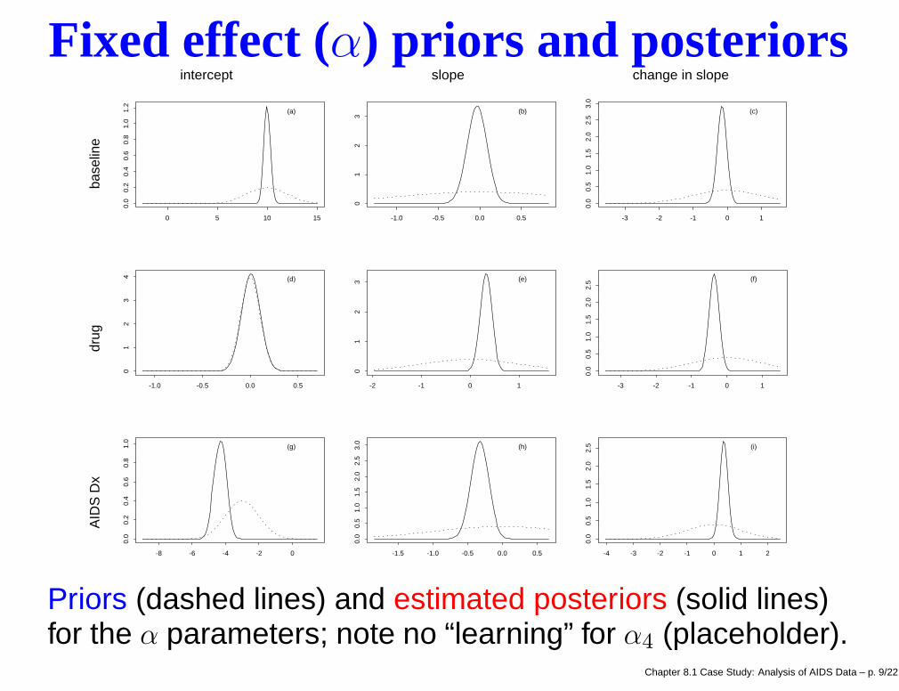
Fixed effect (α) priors and posteriors
0 5 10 15
0.0
0.2
0.4
0.6
0.8
1.0
1.2
(a)
-1.0 -0.5 0.0 0.5
01
23
(b)
-3 -2 -1 0 1
0.0
0.5
1.0
1.5
2.0
2.5
3.0
(c)
-1.0 -0.5 0.0 0.5
01
23
4 (d)
-2 -1 0 1
01
23 (e)
-3 -2 -1 0 1
0.0
0.5
1.0
1.5
2.0
2.5 (f)
-8 -6 -4 -2 0
0.0
0.2
0.4
0.6
0.8
1.0
(g)
-1.5 -1.0 -0.5 0.0 0.5
0.0
0.5
1.0
1.5
2.0
2.5
3.0
(h)
-4 -3 -2 -1 0 1 2
0.0
0.5
1.0
1.5
2.0
2.5 (i)
intercept slope change in slope
AID
S D
x
d
rug
b
asel
ine
Priors (dashed lines) and estimated posteriors (solid lines)for the α parameters; note no “learning” for α4 (placeholder).
Chapter 8.1 Case Study: Analysis of AIDS Data – p. 9/22

Point and interval estimatesmode 95% interval
Baseline intercept α1 9.938 9.319 10.733slope α2 –0.041 –0.285 0.204change in slope α3 –0.166 –0.450 0.118
Drug intercept α4 0.004 –0.190 0.198slope α5 0.309 0.074 0.580change in slope α6 –0.348 –0.671 –0.074
AIDS Dx intercept α7 –4.295 –5.087 –3.609slope α8 –0.322 –0.588 –0.056change in slope α9 0.351 0.056 0.711
ddI trajectories significantly different both before andafter the changepoint
Chapter 8.1 Case Study: Analysis of AIDS Data – p. 10/22

Point and interval estimatesmode 95% interval
Baseline intercept α1 9.938 9.319 10.733slope α2 –0.041 –0.285 0.204change in slope α3 –0.166 –0.450 0.118
Drug intercept α4 0.004 –0.190 0.198slope α5 0.309 0.074 0.580change in slope α6 –0.348 –0.671 –0.074
AIDS Dx intercept α7 –4.295 –5.087 –3.609slope α8 –0.322 –0.588 –0.056change in slope α9 0.351 0.056 0.711
ddI trajectories significantly different both before andafter the changepoint
AIDS Dx main effects also all significantChapter 8.1 Case Study: Analysis of AIDS Data – p. 10/22

Fitted population model by drug and Dx
months after enrollment
squa
re r
oot C
D4
coun
t
02
46
810
0 2 6 12 18
No AIDS Dx at baselineddIddC
AIDS Dx at baseline
Obtained by setting βi = ǫi = 0, α = posterior mode
Chapter 8.1 Case Study: Analysis of AIDS Data – p. 11/22

Fitted population model by drug and Dx
months after enrollment
squa
re r
oot C
D4
coun
t
02
46
810
0 2 6 12 18
No AIDS Dx at baselineddIddC
AIDS Dx at baseline
Obtained by setting βi = ǫi = 0, α = posterior mode
On average, only AIDS-free ddI patients get a “boost”...
But ddC patients “catch up” by the end of the period!Chapter 8.1 Case Study: Analysis of AIDS Data – p. 11/22

Changepoint vs. linear decay model
-2 -1 0 1 2 3
04
812
residuals, Model 1
-2 0 2 4
05
1015
residuals, Model 2
• •
•
•
••
•
••
•
• •
•
•
•
••
• •
•
•
••
•
•
•
•• •
•
•
••
• •
•
•••
•
•
•
••
••
•
••
• •••
•• ••
•
•
•
•• •
••
•
•
•
••
quantiles of standard normal, Model 1
sort
ed r
esid
uals
-2 -1 0 1 2
-20
12
3
••
•
•
••
•
•••
• •
•
•
•
••
• ••
•
••
•
•
•
•••
•
•
••
• •
•
•• •
•
•
•
••••
•
• •• •
••• •
•••
•
•
••••••
•
•
••
quantiles of standard normal, Model 2
sort
ed r
esid
uals
-2 -1 0 1 2
-20
12
3
Model 1: Vinv ~ W(rho = 24 , R = Diag( 4 0.0625 0.0625 )) Model 2: Vinv ~ W(rho = 24 , R = Diag( 4 0.0625 ))
q-q plots indicate a reasonable degree of normality inthese cross validation residuals, rij = yij − E(Yij|y(ij))
Chapter 8.1 Case Study: Analysis of AIDS Data – p. 12/22

Changepoint vs. linear decay model
-2 -1 0 1 2 3
04
812
residuals, Model 1
-2 0 2 4
05
1015
residuals, Model 2
• •
•
•
••
•
••
•
• •
•
•
•
••
• •
•
•
••
•
•
•
•• •
•
•
••
• •
•
•••
•
•
•
••
••
•
••
• •••
•• ••
•
•
•
•• •
••
•
•
•
••
quantiles of standard normal, Model 1
sort
ed r
esid
uals
-2 -1 0 1 2
-20
12
3
••
•
•
••
•
•••
• •
•
•
•
••
• ••
•
••
•
•
•
•••
•
•
••
• •
•
•• •
•
•
•
••••
•
• •• •
••• •
•••
•
•
••••••
•
•
••
quantiles of standard normal, Model 2
sort
ed r
esid
uals
-2 -1 0 1 2
-20
12
3
Model 1: Vinv ~ W(rho = 24 , R = Diag( 4 0.0625 0.0625 )) Model 2: Vinv ~ W(rho = 24 , R = Diag( 4 0.0625 ))
q-q plots indicate a reasonable degree of normality inthese cross validation residuals, rij = yij − E(Yij|y(ij))∑
ij |rij | = 66.37 and 70.82, respectively ⇒ similar fits!Chapter 8.1 Case Study: Analysis of AIDS Data – p. 12/22

Residual and CPO comparison
11
1
1
11
1
11
1
1 1
1
1
1
11
11
1
1
11
1
1
1
1 11
1
1
11
1 1
1
11 1
1
1
1
11
11
1
11
111 1
111 11
1
1
111
11
1
1
1
11
2.1 2.2 2.3 2.4 2.5
-20
12
3
22
2
2
2
2
2
22
2
2 2
2
2
2
22
222
2
22
2
2
2
222
2
2
22
2 2
2
22 2
2
2
2
22 22
2
22
22
2 22 2
2 22
2
2
2222
22
2
2
22
a) y_r - E(y_r) versus sd(y_r); plotting character indicates model number
••
•
•
•
•••
•
•
••
•
•
• • •
•
• •
•••
••
••
••
•
•
• •
•••
•••
•
•
•
••
•
•••
•• •
••• • •••
•
•
••
••••
•
•
••
Model 1
Mod
el 2
0.08 0.10 0.12 0.14 0.16 0.18
0.04
0.10
0.16
b) Comparison of CPO values
reduction in rij from Model 2 (linear) to Model 1(changepoint) is negligible
Chapter 8.1 Case Study: Analysis of AIDS Data – p. 13/22

Residual and CPO comparison
11
1
1
11
1
11
1
1 1
1
1
1
11
11
1
1
11
1
1
1
1 11
1
1
11
1 1
1
11 1
1
1
1
11
11
1
11
111 1
111 11
1
1
111
11
1
1
1
11
2.1 2.2 2.3 2.4 2.5
-20
12
3
22
2
2
2
2
2
22
2
2 2
2
2
2
22
222
2
22
2
2
2
222
2
2
22
2 2
2
22 2
2
2
2
22 22
2
22
22
2 22 2
2 22
2
2
2222
22
2
2
22
a) y_r - E(y_r) versus sd(y_r); plotting character indicates model number
••
•
•
•
•••
•
•
••
•
•
• • •
•
• •
•••
••
••
••
•
•
• •
•••
•••
•
•
•
••
•
•••
•• •
••• • •••
•
•
••
••••
•
•
••
Model 1
Mod
el 2
0.08 0.10 0.12 0.14 0.16 0.18
0.04
0.10
0.16
b) Comparison of CPO values
reduction in rij from Model 2 (linear) to Model 1(changepoint) is negligible
CPO’s are usually larger for Model 1, but not much
⇒ CD4 counts adequately explained by the linear model!Chapter 8.1 Case Study: Analysis of AIDS Data – p. 13/22

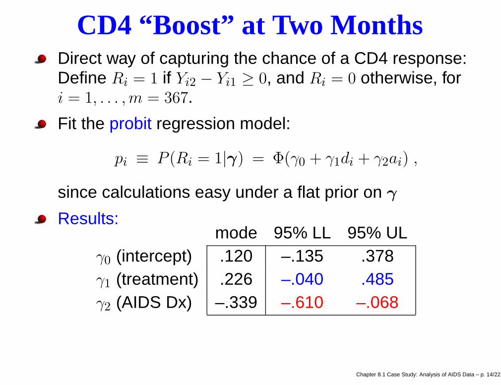
CD4 “Boost” at Two MonthsDirect way of capturing the chance of a CD4 response:Define Ri = 1 if Yi2 − Yi1 ≥ 0, and Ri = 0 otherwise, fori = 1, . . . ,m = 367.
Chapter 8.1 Case Study: Analysis of AIDS Data – p. 14/22

CD4 “Boost” at Two MonthsDirect way of capturing the chance of a CD4 response:Define Ri = 1 if Yi2 − Yi1 ≥ 0, and Ri = 0 otherwise, fori = 1, . . . ,m = 367.
Fit the probit regression model:
pi ≡ P (Ri = 1|γ) = Φ(γ0 + γ1di + γ2ai) ,
since calculations easy under a flat prior on γ
Chapter 8.1 Case Study: Analysis of AIDS Data – p. 14/22
CD4 “Boost” at Two MonthsDirect way of capturing the chance of a CD4 response:Define Ri = 1 if Yi2 − Yi1 ≥ 0, and Ri = 0 otherwise, fori = 1, . . . ,m = 367.
Fit the probit regression model:
pi ≡ P (Ri = 1|γ) = Φ(γ0 + γ1di + γ2ai) ,
since calculations easy under a flat prior on γ
Results:mode 95% LL 95% UL
γ0 (intercept) .120 –.135 .378γ1 (treatment) .226 –.040 .485γ2 (AIDS Dx) –.339 –.610 –.068
Chapter 8.1 Case Study: Analysis of AIDS Data – p. 14/22

CD4 “Boost” at Two MonthsDirect way of capturing the chance of a CD4 response:Define Ri = 1 if Yi2 − Yi1 ≥ 0, and Ri = 0 otherwise, fori = 1, . . . ,m = 367.
Fit the probit regression model:
pi ≡ P (Ri = 1|γ) = Φ(γ0 + γ1di + γ2ai) ,
since calculations easy under a flat prior on γ
Results:mode 95% LL 95% UL
γ0 (intercept) .120 –.135 .378γ1 (treatment) .226 –.040 .485γ2 (AIDS Dx) –.339 –.610 –.068
⇒ Boost more likely for patients without an AIDS Dx and(to a lesser extent) taking ddI
Chapter 8.1 Case Study: Analysis of AIDS Data – p. 14/22

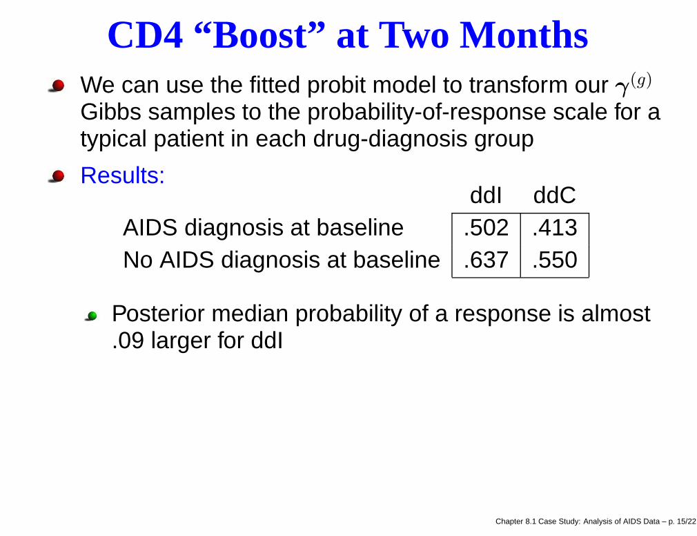
CD4 “Boost” at Two MonthsWe can use the fitted probit model to transform our γ(g)
Gibbs samples to the probability-of-response scale for atypical patient in each drug-diagnosis group
Chapter 8.1 Case Study: Analysis of AIDS Data – p. 15/22

CD4 “Boost” at Two MonthsWe can use the fitted probit model to transform our γ(g)
Gibbs samples to the probability-of-response scale for atypical patient in each drug-diagnosis group
Results:ddI ddC
AIDS diagnosis at baseline .502 .413No AIDS diagnosis at baseline .637 .550
Chapter 8.1 Case Study: Analysis of AIDS Data – p. 15/22
CD4 “Boost” at Two MonthsWe can use the fitted probit model to transform our γ(g)
Gibbs samples to the probability-of-response scale for atypical patient in each drug-diagnosis group
Results:ddI ddC
AIDS diagnosis at baseline .502 .413No AIDS diagnosis at baseline .637 .550
Posterior median probability of a response is almost.09 larger for ddI
Chapter 8.1 Case Study: Analysis of AIDS Data – p. 15/22

CD4 “Boost” at Two MonthsWe can use the fitted probit model to transform our γ(g)
Gibbs samples to the probability-of-response scale for atypical patient in each drug-diagnosis group
Results:ddI ddC
AIDS diagnosis at baseline .502 .413No AIDS diagnosis at baseline .637 .550
Posterior median probability of a response is almost.09 larger for ddIAIDS-negative patients have a .135 larger chance ofresponding than an AIDS-positive patient
But for even the best response group (AIDS-free ddIpatients), there is a substantial estimated probability ofnot experiencing a boost
Chapter 8.1 Case Study: Analysis of AIDS Data – p. 15/22
Survival AnalysisDoes the CD4 “boost” translate into an improvement insurvival?
Chapter 8.1 Case Study: Analysis of AIDS Data – p. 16/22

Survival AnalysisDoes the CD4 “boost” translate into an improvement insurvival?
To check, fit a proportional hazards model:
h(t|z,β) = h0(t) exp(z′β)
where we employ the covariates
Chapter 8.1 Case Study: Analysis of AIDS Data – p. 16/22

Survival AnalysisDoes the CD4 “boost” translate into an improvement insurvival?
To check, fit a proportional hazards model:
h(t|z,β) = h0(t) exp(z′β)
where we employ the covariatesz0 = 1 for all patients
Chapter 8.1 Case Study: Analysis of AIDS Data – p. 16/22

Survival AnalysisDoes the CD4 “boost” translate into an improvement insurvival?
To check, fit a proportional hazards model:
h(t|z,β) = h0(t) exp(z′β)
where we employ the covariatesz0 = 1 for all patientsz1 = 1 for ddI patients with a CD4 response, and 0otherwise
Chapter 8.1 Case Study: Analysis of AIDS Data – p. 16/22

Survival AnalysisDoes the CD4 “boost” translate into an improvement insurvival?
To check, fit a proportional hazards model:
h(t|z,β) = h0(t) exp(z′β)
where we employ the covariatesz0 = 1 for all patientsz1 = 1 for ddI patients with a CD4 response, and 0otherwisez2 = 1 for ddC patients without a CD4 response, and0 otherwise
Chapter 8.1 Case Study: Analysis of AIDS Data – p. 16/22

Survival AnalysisDoes the CD4 “boost” translate into an improvement insurvival?
To check, fit a proportional hazards model:
h(t|z,β) = h0(t) exp(z′β)
where we employ the covariatesz0 = 1 for all patientsz1 = 1 for ddI patients with a CD4 response, and 0otherwisez2 = 1 for ddC patients without a CD4 response, and0 otherwisez3 = 1 for ddC patients with a CD4 response, and 0otherwise
Chapter 8.1 Case Study: Analysis of AIDS Data – p. 16/22

Survival AnalysisLoglikelihood (Cox and Oakes, 1984):
log L(β) =∑
i∈U
log h(ti|zi,β) +m∑
i=1
log S(ti|zi,β) ,
where
Chapter 8.1 Case Study: Analysis of AIDS Data – p. 17/22
Survival AnalysisLoglikelihood (Cox and Oakes, 1984):
log L(β) =∑
i∈U
log h(ti|zi,β) +m∑
i=1
log S(ti|zi,β) ,
whereh denotes the hazard function
Chapter 8.1 Case Study: Analysis of AIDS Data – p. 17/22

Survival AnalysisLoglikelihood (Cox and Oakes, 1984):
log L(β) =∑
i∈U
log h(ti|zi,β) +m∑
i=1
log S(ti|zi,β) ,
whereh denotes the hazard functionS denotes the survival function
Chapter 8.1 Case Study: Analysis of AIDS Data – p. 17/22

Survival AnalysisLoglikelihood (Cox and Oakes, 1984):
log L(β) =∑
i∈U
log h(ti|zi,β) +m∑
i=1
log S(ti|zi,β) ,
whereh denotes the hazard functionS denotes the survival functionU the collection of uncensored failure times(observed deaths), and
Chapter 8.1 Case Study: Analysis of AIDS Data – p. 17/22

Survival AnalysisLoglikelihood (Cox and Oakes, 1984):
log L(β) =∑
i∈U
log h(ti|zi,β) +m∑
i=1
log S(ti|zi,β) ,
whereh denotes the hazard functionS denotes the survival functionU the collection of uncensored failure times(observed deaths), andzi = (z0i, z1i, z2i, z3i)
′
Our parametrization uses nonresponding ddI patientsas a reference group; β1, β2, and β3 capture the effect ofbeing in one of the other 3 drug-response groups.
Chapter 8.1 Case Study: Analysis of AIDS Data – p. 17/22

Survival AnalysisBegin with a parametric baseline hazard, say Weibull:
h0(t) = ρtρ−1
Chapter 8.1 Case Study: Analysis of AIDS Data – p. 18/22

Survival AnalysisBegin with a parametric baseline hazard, say Weibull:
h0(t) = ρtρ−1
Result: extremely high posterior correlation between ρand β0! So fix ρ = 1 (return to constant baseline hazard,i.e., an exponential survival model).
Chapter 8.1 Case Study: Analysis of AIDS Data – p. 18/22

Survival AnalysisBegin with a parametric baseline hazard, say Weibull:
h0(t) = ρtρ−1
Result: extremely high posterior correlation between ρand β0! So fix ρ = 1 (return to constant baseline hazard,i.e., an exponential survival model).
Resulting posterior quantiles:
median 95% LL 95% ULβ0 (baseline) –7.00 –7.34 –6.67β1 (ddI resp) –.07 –.54 .38β2 (ddC nonresp) .06 –.39 .53β2 (ddC resp) –.53 –1.10 .02
⇒ only the ddC responders seem different!Chapter 8.1 Case Study: Analysis of AIDS Data – p. 18/22

Survival Analysis
Typical nice feature of parametric MCMC analysis:Our posterior γ(g) samples may be easily transformedto investigate:
Chapter 8.1 Case Study: Analysis of AIDS Data – p. 19/22

Survival Analysis
Typical nice feature of parametric MCMC analysis:Our posterior γ(g) samples may be easily transformedto investigate:
the survival function at time t:
S(t|z,β) = exp{−t exp(z′β)} ,
or
Chapter 8.1 Case Study: Analysis of AIDS Data – p. 19/22
Survival Analysis
Typical nice feature of parametric MCMC analysis:Our posterior γ(g) samples may be easily transformedto investigate:
the survival function at time t:
S(t|z,β) = exp{−t exp(z′β)} ,
orthe median survival time:
θ(z,β) = (log 2) exp(−z′β)
(set S(t|z,β) = 1/2 and solve for t)
Chapter 8.1 Case Study: Analysis of AIDS Data – p. 19/22

EstimatedS(t) and median survival
days since randomization
prop
ortio
n re
mai
ning
aliv
e
0 200 400 600 800
0.0
0.4
0.8
ddI, no CD4 boostddI, CD4 boostddC, no CD4 boostddC, CD4 boost
(a)
days since randomization
post
erio
r de
nsity
500 1000 1500 2000
0.0
0.00
2
ddI, no CD4 boostddI, CD4 boostddC, no CD4 boostddC, CD4 boost
(b)
Fitted survival for ddC responders stands out
Chapter 8.1 Case Study: Analysis of AIDS Data – p. 20/22

EstimatedS(t) and median survival
days since randomization
prop
ortio
n re
mai
ning
aliv
e
0 200 400 600 800
0.0
0.4
0.8
ddI, no CD4 boostddI, CD4 boostddC, no CD4 boostddC, CD4 boost
(a)
days since randomization
post
erio
r de
nsity
500 1000 1500 2000
0.0
0.00
2
ddI, no CD4 boostddI, CD4 boostddC, no CD4 boostddC, CD4 boost
(b)
Fitted survival for ddC responders stands out
Difference is even more dramatic on the mediansurvival time scale (lower panel)
⇒ Clinically significant improvement in survival only forddC patients experiencing a boost!
Chapter 8.1 Case Study: Analysis of AIDS Data – p. 20/22

Conclusions
ddC is less successful than ddI in producing a CD4boost in patients with advanced HIV infection, BUT...
Chapter 8.1 Case Study: Analysis of AIDS Data – p. 21/22

Conclusions
ddC is less successful than ddI in producing a CD4boost in patients with advanced HIV infection, BUT...
This superior CD4 performance does not seem totranslate into improved survival.
Chapter 8.1 Case Study: Analysis of AIDS Data – p. 21/22

Conclusions
ddC is less successful than ddI in producing a CD4boost in patients with advanced HIV infection, BUT...
This superior CD4 performance does not seem totranslate into improved survival.
That is, CD4 is prognostic, but not a surrogate endpoint.
Recommendations
Chapter 8.1 Case Study: Analysis of AIDS Data – p. 21/22

Conclusions
ddC is less successful than ddI in producing a CD4boost in patients with advanced HIV infection, BUT...
This superior CD4 performance does not seem totranslate into improved survival.
That is, CD4 is prognostic, but not a surrogate endpoint.
RecommendationsRethink the practice of licensing drugs basedprimarily on an increase in CD4 count.
Chapter 8.1 Case Study: Analysis of AIDS Data – p. 21/22

Conclusions
ddC is less successful than ddI in producing a CD4boost in patients with advanced HIV infection, BUT...
This superior CD4 performance does not seem totranslate into improved survival.
That is, CD4 is prognostic, but not a surrogate endpoint.
RecommendationsRethink the practice of licensing drugs basedprimarily on an increase in CD4 count.Review the use of these drugs with end-stagepatients (low efficacy, unpleasant side effects)
Chapter 8.1 Case Study: Analysis of AIDS Data – p. 21/22

Conclusions
ddC is less successful than ddI in producing a CD4boost in patients with advanced HIV infection, BUT...
This superior CD4 performance does not seem totranslate into improved survival.
That is, CD4 is prognostic, but not a surrogate endpoint.
RecommendationsRethink the practice of licensing drugs basedprimarily on an increase in CD4 count.Review the use of these drugs with end-stagepatients (low efficacy, unpleasant side effects)Reconsider placebo trials?!?
Chapter 8.1 Case Study: Analysis of AIDS Data – p. 21/22

Medical journal references:
“Main paper”: ABRAMS, D.I., GOLDMAN, A.I., ET AL. (1994).Comparative trial of didanosine and zalcitabine inpatients with human immunodeficiency virus infectionwho are intolerant of or have failed zidovudine therapy.New England Journal of Medicine, 330, 657–662.
Chapter 8.1 Case Study: Analysis of AIDS Data – p. 22/22

Medical journal references:
“Main paper”: ABRAMS, D.I., GOLDMAN, A.I., ET AL. (1994).Comparative trial of didanosine and zalcitabine inpatients with human immunodeficiency virus infectionwho are intolerant of or have failed zidovudine therapy.New England Journal of Medicine, 330, 657–662.
Bayesian followup paper: GOLDMAN, A.I., CARLIN, B.P.,CRANE, L.R., LAUNER, C., KORVICK, J.A., DEYTON, L., AND
ABRAMS, D.I. (1996). Response of CD4 lymphocytes andclinical consequences of treatment using ddI or ddC inpatients with advanced HIV infection. Journal ofAcquired Immune Deficiency Syndromes and HumanRetrovirology, 11, 161–169.
Chapter 8.1 Case Study: Analysis of AIDS Data – p. 22/22


![ADAPTIVE CRUISE CONTROL OF A SIMSCAPE DRIVELINE …jestec.taylors.edu.my/Vol 16 issue 1 February 2021/16_1_47.pdflongitudinal vehicle dynamics using Simscape Driveline library [36]](https://img.pdfslide.net/doc/110x75/612eb33c1ecc51586942faa7/adaptive-cruise-control-of-a-simscape-driveline-16-issue-1-february-202116147pdf.jpg)