Loop Equations and bootstrapmethods in the lattice

Peter D. Anderson1,2 and Martin Kruczenski1 ∗1 Department of Physics and Astronomy, Purdue U.,

525 Northwestern Avenue, W. Lafayette, IN 47907-2036, USA2 Wigner Research Center for Physics of the HAS,

29–33 Konkoly–Thege Miklos Str. H-1121 Budapest, Hungary

September 24, 2018

Abstract

Pure gauge theories can be formulated in terms of Wilson Loopscorrelators by means of the loop equation. In the large-N limit thisequation closes in the expectation value of single loops. In particular,using the lattice as a regulator, it becomes a well defined equationfor a discrete set of loops. In this paper we study different numer-ical approaches to solving this equation. Previous ideas gave goodresults in the strong coupling region. Here we propose an alternativemethod based on the observation that certain matrices ρ of Wilsonloop expectation values are positive definite. They also have unittrace (ρ � 0,Trρ = 1), in fact they can be defined as density matricesin the space of open loops after tracing over color indices and can beused to define an entropy associated with the loss of information dueto such trace SWL = −Tr[ρ ln ρ]. The condition that such matricesare positive definite allows us to study the weak coupling region whichis relevant for the continuum limit. In the exactly solvable case of twodimensions this approach gives very good results by considering justa few loops. In four dimensions it gives good results in the weak cou-pling region and therefore is complementary to the strong couplingexpansion. We compare the results with standard Monte Carlo simu-lations.

∗E-mail: ander324@purdue.edu, markru@purdue.edu

1

arX

iv:1

612.

0814

0v2

[he

p-th

] 1

4 Ja

n 20

17

1 Introduction

Gauge theories are of fundamental importance for our understanding of Na-ture but many of their properties are still mysterious, for example in puregauge theories, the phenomenon of confinement is still not fully understood.Even further, the AdS/CFT correspondence [1] has shown that gauge theo-ries in the strongly coupled regime can be described equally well in terms ofstring theory in a higher dimensional space. That means that certain gaugetheories contain quantum gravity, emergent space-time and strings as boundstates. Fundamental to this understanding is the relation of gauge theoriesand string theory in the limit of a large number of colors as envisioned by’t Hooft [2]. In such relation, exemplified by AdS/CFT, the string theorydescription is completely in terms of gauge invariant operators. In fact thegauge symmetry is not a symmetry of the dual theory in accordance withthe usual understanding that a gauge symmetry is a manifestation of redun-dant degrees of freedoms that have to be eliminated. Taken to its logicalconclusion, the principle of gauge invariance cannot be used as the basis toconstruct such a theory and perhaps more ideas are needed to understandthe fundamental principles lying behind gauge theories.

For these reasons it is natural to study gauge invariant formulations ofgauge theories. In fact it is known that gauge theories can be formulatedentirely in terms of Wilson loops. In particular, in the large-N limit Wilsonloops obey an equation that closes in the expectation value of single Wilsonloops. This is known as the loop equation [3, 4] or the Migdal–Makeenkoequation. For finite N the equation is also valid but closes in the expectationvalue of disconnected (i.e. multitrace) Wilson loops. Since it is not clearhow to renormalize the loop equation it can be better study perturbativelyor in the lattice. Motivated by this, here we discuss different numerical andanalytical methods to study the loop equation in the lattice.

Although, as we argued, this equation is of great importance there doesnot seem to be many studies on how to solve it. A notable exception is thevery interesting work by Marchesini [5] where a formal solution and a nu-merical approach to solve the loop equation was proposed. We discuss thisapproach in detail but unfortunately it seems restricted to the strongly cou-pled regime, moreover, and the known numerical results are for the 2d case.The method we propose is based on the observation that certain matricesconstructed of Wilson loop expectation values are positive definite. Theycan be thought of as reduced density matrices in the space of open loops

2

after tracing over color indices. Imposing this extra condition allow us to se-lect valid solutions of the loop equations. We call this approach a bootstrapapproach since it uses general positivity properties of the theory to imposebounds on the solutions and also since imposing positive definiteness is animportant part of the recently developed and highly successful conformalbootstrap program [6, 7]1. The bounds we impose are for the expectationvalue of the energy. In two dimensions such bounds constrain the solution tobe equal to the exact solution with high degree of accuracy. In four dimen-sions the bounds are less restrictive (due to larger computational complexity)but we can resort to a simple approximation, at small coupling we minimizethe expectation value of the energy subject to the constraints, whereas atlarge coupling the entropy should be maximized. This gives results whichare in good agreement with simulations and a reasonable approximation tothe coupling where the transition occurs. The weak coupling region is welldescribed by this method although, at the moment, this is not enough tounderstand the continuum limit.

For future work, it seems of great interest to apply this method to N = 4SYM in order to make contact with the AdS/CFT correspondence. In thispaper we take a few initial steps in this direction by briefly considering thebosonic sector of N = 4 SYM but leave a detailed study for future work.

It is interesting to note that the relevance of the extra positivity conditionsat weak coupling was already observed [9] in the collective field methodof Jevicki and Sakita [10]. Using the Kogut-Susskind approach a LatticeHamiltonian in loop space was derived and numerically studied in [9]. Seealso the related work by Yaffe [11] using coherent states.

This paper is organized as follows, in the next section we review thederivation of the loop equation and summarize the main ideas presented inthis paper, following that we consider in great detail the two dimensional casesince its solution is known exactly and can be used to test various approachesvery easily. Afterwards, we apply those ideas to the four dimensional case andshow that our numerical approach gives a good understanding of the gaugetheory in the small coupling regime relevant for the continuum limit. Finallywe describe a numerical simulation used to validate the results, discuss brieflythe case of N = 4 SYM and conclude with a summary of the results and

1We want to clarify however, that the ideas discussed here do not seem to have anyrelation with conformal symmetry. Perhaps closer is the idea of applying the bootstrapmethod to non-conformal theories [8] but we do not know of any direct relation with thepresent work.

3

possible extensions and improvements.

2 Lattice gauge theory, a brief summary.

In this section we consider a four dimensional SU(N) gauge theory in aninfinite cubic lattice with Wilson action and briefly review known results forthe large N limit. Then we discuss the derivation of the loop equation andintroduce the notation we use in this paper. There is an extensive literatureon the subject, our presentation here is just to summarize known results thatare needed later in the paper and mostly follow the classic review [12] andthe book [13] as regards to the loop equation.

2.1 Lattice action and known results

The system we consider is a cubic lattice where to each oriented link isassociated a matrix Uµ ∈ SU(N). To the same link with opposite orientationwe associate the matrix Uµ = U †µ. The action is the Wilson action

S = −N2λ

∑P

TrUP , (2.1)

where the sum is over all oriented plaquettes P . Here UP is the product ofthe four matrices associated with the plaquette and oriented means that wesum the trace of both possible orientation so that the action is real. Thepartition function is

Z =

∫ ∏~x,µ

dUµ(~x) e−S. (2.2)

In four dimensions, for N ≥ 4 numerical results indicate that this theory hasa first order phase transition as a function of λ [12]. In the large-N limitthe transition occurs at λc = 1.3904, as computed using the Twisted Eguchi-Kawai (TEK) model[14]. The nature of the transition is easily understoodby considering the partition function in eq.(2.2) as defining a classical fourdimensional statistical system with Hamiltonian

H = −N2

∑P

TrUP , (2.3)

4

and temperature T = λ. At small temperature λ → 0 we minimize the en-ergy, i.e. the links Uµ fluctuate around gauge trivial configurations. At largetemperature λ→∞ the entropy should be maximized and the links variablesUµ explore all possible values with equal probability. Thus, the transition isa typical first order first transition between ordered and disordered states.

The large coupling phase is confining and easily studied analytically interms of a strong coupling expansion already proposed by Wilson[15]. Onthe other hand the continuum limit is obtained in the region λ → 0 whichis more difficult to study. A Wilson loop expectation value is a real numberassociated with a closed path in the lattice and defined as

WC =1

Z

∫ ∏~xµ

dUµ(~x)1

NTr(Uµ1 . . . UµL)e−S , (2.4)

where inside the trace we multiplied in cyclic order all the matrices associatedto the given path C = {µ1µ2 . . . µL}.

2.1.1 Strong coupling phase

Analytically, the Wilson loop expectation values WC can be compute in astrong coupling expansion λ � 1 by expanding the exponential of the ac-tion. The result has an interesting interpretation in terms of a sum oversurfaces ending on the loop [16]. In 4 dimensions and in the large N-limitthe expectation value for the plaquette is given by

W1 = u =1

2λ+

1

8λ5+

15

128

1

λ9+

17

256

1

λ11+

273

2048

1

λ13+

185

1024

1

λ15+ . . . (2.5)

where we called the plaquette as Wilson loop one W1 also denoted as u.Wilson loop zero is the single point or null loop that obeys W0 = 1. Suchlarge orders in perturbation theory can be computed by using a characterexpansion of the exponential. Notice thatW1 = u is of particular importancesince it determines the average Energy density (energy per lattice site)

E

V N2= −6u , (2.6)

where V is the number of sites and the factor six is the number of plaquettesper site computed as d(d− 1)/2, in dimension d = 4.

5

2.1.2 Weak coupling

For small coupling the Uµ matrices only have small fluctuations around theidentity (up to gauge transformations). In that case one can write the theoryin terms of a hermitian gauge field Aµ, Uµ = eiAµ and use Feynman diagramsto compute Wilson loops. The result for the plaquette in four dimensionsand the large N limit is [17]

W1 = u = 1− λ

4−(

1

48+ c2

)λ2, c2 ' −0.00041 . (2.7)

Of course perturbation becomes unreliable for loops of large area since it doesnot capture the phenomenon of confinement that implies that such loops obeythe area law.

2.1.3 Transition in mean field approximation

The transition from weak to the strong coupling regime is a first order tran-sition that can be understood by a simple mean field approximation [12].Within this approximation and in axial gauge, the free energy per site isgiven by [12]

a = − λ

V N2lnZ =

{3(1− 1

λ

)v2 − 3

λv4 0 < v < 1

234− 3

2ln(2(1− v))− 3

λ(v4 + v2) 1

2< v < 1 ,

(2.8)where v is a free parameter that is fixed by minimizing a, i.e.∂a

∂v= 0. The

function a(v) has a minimum at v = 0 and for λ < λM ' 1.68 has a sec-ond minimum corresponding to the small coupling phase that has lower freeenergy for λ < λc ' 1.48. The expectation value of the plaquette is given by

u = −1

6

(a− λ∂a

∂λ

)=

1

2(v2 + v4) , (2.9)

as can be derived from the partition function. In the strong coupling regimewe get the very crude approximation u = 0, in fact all Wilson loops vanish. Inthe small coupling regime we get a non-trivial function that can be expandedaround λ = 0 as

u = 1− 1

4λ+ . . . (2.10)

This agrees with eq.(2.7) but the λ2 term (− 7288λ2 ) is already incorrect.

The mean field approximation can be improved [12] but we just wanted toemphasize that a simple approach captures the important physics.

6

0

0.2

0.4

0.6

0.8

1

0 0.5 1 1.5 2 2.5 3

uMonte Carlo Data

Weak CouplingStrong Coupling

MC N=10

Figure 1: Monte Carlo results for the plaquette verse the t’ Hooft coupling

2.1.4 Numerical simulations

All previous results are for infinite lattices and in the strict N →∞ limit. Forfinite N and small lattices one can use numerical simulations and extrapolatethe results to infinite N. The first results in this direction were by Creutz andMoriarty [18] and more recently by Meyer and Teper [19]. As part of thiswork we performed a numerical simulation for N = 10 in an 84 lattice whichallowed us to check various ideas regarding the loop equation. The resultsfor the expectation value of the plaquette are displayed in fig.1 where a verygood agreement is seen with the perturbative and large coupling expansionin their regimes of validity. The position of the phase transition for SU(10)is seen to be around λc(N = 10) ' 1.46 in agreement with the literature andclose to the large-N value λc ' 1.3904 [14].

2.1.5 Summary

Clearly there is already a very good and detailed understanding of this sys-tem, the strong and weak coupling regimes can be understood by series ex-pansion and the transition using mean field. Numerical simulations validatethe whole picture as summarized in fig.1. It should be emphasized however

7

that the main physical interest lies in the continuum limit that appears in theλ→ 0 region. In practice one has to show that large loops obey the area lawin the weak coupling phase, a result that cannot be obtained by perturbationtheory and can only be found by extrapolation of numerical simulations.

In any case, our intention here is to study this system purely in terms ofgauge invariant operators, namely with no reference to the variables Uµ. Forthat reason we review now the derivation of the loop equation.

2.2 The loop equation

The loop equation is a direct consequence of the Schwinger-Dyson equationassociated with a link of the lattice [3, 4, 13]. We reproduce its derivationhere, first to introduce the notation, and second because for other theories thederivation will be done just by analogy to this one. Consider then a point ~xin the lattice and a given link µ = 0, 1, 2, 3, and perform the following changeof variables

Uµ → (1 + iε)Uµ, U †µ → U †µ(1− iε), ε† = ε, Trε = 0 . (2.11)

The variation of the action is

δS = −N2λ

∑±ν 6=µ

(iεabW

ab{µνµν} − iεabW ba{νµνµ}), (2.12)

where W ab{µνµν} indicates a Wilson line made of four links starting andending at ~x and following the directions {µνµν} where the bar indicatesthat the link is traversed in the opposite direction as µ. Let us perform thischange of variables in the integral∫

DU δε

(e−S W ab

~x {µ, C})

= 0 , (2.13)

where W ab~x {µ, C} indicates a Wilson line starting at point ~x in direction µ

and then coming back to ~x along some given path C that in principle maypass again through the same link ~x, µ in the positive or negative direction.Since the change of variables does not change the value of the integral, thevariation vanishes which can be expressed in the usual form

〈−δεS W ab~x 〉+ 〈δεW ab

~x 〉 = 0 . (2.14)

8

Explicitly

iN

2λ〈∑±ν 6=µ

(εcdW

dc{µνµν} − εcdW dc{νµνµ})W ab~x {µ, C}〉+ iεad〈W db

~x 〉

+〈n+∑j+=1

iW ac~x~x+ε

cdW db~x+~x〉 − 〈

n−∑j−=1

iW ac~x~x−ε

cdW db~x−~x〉 = 0 , (2.15)

where the terms in the last line come from the possibility that the pathgoes through the same link again either in the same direction (n+ times), oropposite direction (n− times). These terms are call self-intersection terms butnotice that self-intersection in this context means that the loop goes throughthe same link more than once (in either direction) and not merely throughthe same vertex. Since this identity is valid for any traceless hermitian ε weconclude (εcdA

dc = 0⇒ Acd = δcd 1NAaa)

N

2λ〈∑±ν 6=µ

W dc~x {µνµν}W ab

~x {µ, C} −W dc~x {νµνµ}W ab

~x {µ, C}〉+ δac〈W db~x 〉

+〈n+∑j+=1

W ac~x~x+W

db~x+~x〉 − 〈

n−∑j−=1

W ac~x~x−W

db~x−~x〉 (2.16)

= δcd

[1

2λ〈∑±ν 6=µ

W~x{µνµν}W ab~x {µ, C} −W~x{νµνµ}W ab

~x {µ, C}〉+1

N〈W ab

~x 〉

+1

N(n+ − n−)〈W ab

~x 〉]. (2.17)

Contracting both sides with δacδbd we get

N

2λ

∑±ν 6=µ

〈W~x{µνµνµC} −W~x{νµνC}〉+N〈W~x〉

+

n+∑j+=1

〈W~x~x+W~x+~x〉 −n−∑j−=1

〈W~x~x−W~x−~x〉 = (2.18)

1

2λ〈∑±ν 6=µ

W~x{µνµν}W~x −W~x{νµνµ}W~x〉+1

N(n+ − n− + 1)〈W~x〉 ,

9

Figure 2: Intersection with the action S ∗W term. In this case the action issimply given by a plaquette. Curvy lines represent schematically the rest ofthe loop.

Figure 3: Self intersection terms. It only appears if the Wilson loop traversesthe same link more than once (in the same or opposite directions). The firsttype gives a positive contribution, the second one a negative one.

a useful form of the loop equation associated with each link of the loop. Inthe large N limit, we divide both sides by N2 and get

1

2λ

∑±ν 6=µ

W~x{µνµνµC}−W~x{νµνC}+W~x+

n+∑j+=1

W~x~x+W~x+~x−n−∑j−=1

W~x~x−W~x−~x = 0 ,

(2.19)where we defined

W{C} =1

N〈W{C}〉 , (2.20)

and used the large N factorization property

1

N2〈W{C1}W{C2}〉 =W{C1}W{C2}+O(

1

N2) . (2.21)

The different terms in the result have a very simple graphical interpretationas seen in figs.(2,3). The link ~x, µ appears in the action in several plaquettes.Each of these plaquettes is connected to the loop as in the figure, when the

10

orientations are opposite, we include a minus sign. Also the action comeswith a coefficient N

2λ. Summing over all links we get the loop equation that

we schematically write as

− 1

NLS ∗W +W +

1

L

∑i

σiW1iW2i = 0 , (2.22)

where L denotes the length of the loop, S∗W denotes all possible intersectionsbetween the loops appearing in the Wilson loop (at a fixed position) and thoseappearing in the action. The last term is a sum over all self-intersections witha sign σi depending on the orientation of the intersection and C1 and C2 denotethe two loops in which the original loop splits when reconnecting at that self-intersection (see fig.3). In this form the loop equation is valid for any actiongiven by a sum of Wilson loops. Therefore, we can give a linear combinationof loops as the action and the reconnection procedure determines completelythe loop equation without any reference to matrices, gauge invariance etc.

For mathematical manipulations it is convenient to enumerate the loopsin a list, where we eliminate redundancy due to rotations, translations, cyclicpermutations and opposite orientations. The first few elements of the list arein fig.(4). Then we can write the loop equation in the form

Ki→jWj + 2λWi + 2λCi→jkWjWk = δi1 , (2.23)

whereWi denotes the expectation value of loop i, Ki→j is a matrix indicatingthat loop i converts into loop j by the reconnection procedure of the actionwith a weight depending on how many different ways we can get j and dividedby the length of the loop L. The tensor Ci→jk is the self-intersection termand indicates that Wilson loop i splits into jk with an appropriate coefficient.For example, for the plaquette we get

−W0 −W2 − 4W3 +W17 +W20 + 4W21 + 2λW1 = 0 . (2.24)

2.3 Extra equations

From the derivation of the previous subsection it is clear that we can getmore equations than just the loop equation. First we can obtain individualSchwinger–Dyson equations for each link. Given two links that do not belongto a self-intersection, the difference between their respective equations islinear and independent of λ. Other linear lambda-independent equations can

11

(1)

(20)(17)

(4)(3)(2)

(6)

(21)(18)

(14)(16)

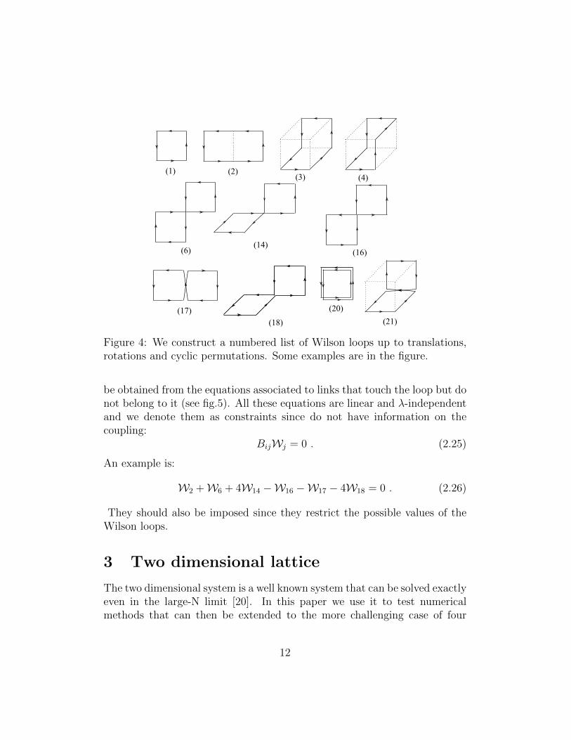
Figure 4: We construct a numbered list of Wilson loops up to translations,rotations and cyclic permutations. Some examples are in the figure.

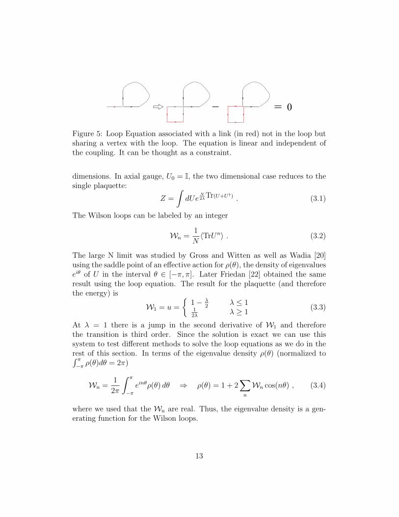
be obtained from the equations associated to links that touch the loop but donot belong to it (see fig.5). All these equations are linear and λ-independentand we denote them as constraints since do not have information on thecoupling:

BijWj = 0 . (2.25)

An example is:

W2 +W6 + 4W14 −W16 −W17 − 4W18 = 0 . (2.26)

They should also be imposed since they restrict the possible values of theWilson loops.

3 Two dimensional lattice

The two dimensional system is a well known system that can be solved exactlyeven in the large-N limit [20]. In this paper we use it to test numericalmethods that can then be extended to the more challenging case of four

12

0

Figure 5: Loop Equation associated with a link (in red) not in the loop butsharing a vertex with the loop. The equation is linear and independent ofthe coupling. It can be thought as a constraint.

dimensions. In axial gauge, U0 = I, the two dimensional case reduces to thesingle plaquette:

Z =

∫dUe

N2λ

Tr(U+U†) . (3.1)

The Wilson loops can be labeled by an integer

Wn =1

N〈TrUn〉 . (3.2)

The large N limit was studied by Gross and Witten as well as Wadia [20]using the saddle point of an effective action for ρ(θ), the density of eigenvalueseiθ of U in the interval θ ∈ [−π, π]. Later Friedan [22] obtained the sameresult using the loop equation. The result for the plaquette (and thereforethe energy) is

W1 = u =

{1− λ

2λ ≤ 1

12λ

λ ≥ 1(3.3)

At λ = 1 there is a jump in the second derivative of W1 and thereforethe transition is third order. Since the solution is exact we can use thissystem to test different methods to solve the loop equations as we do in therest of this section. In terms of the eigenvalue density ρ(θ) (normalized to∫ π−π ρ(θ)dθ = 2π)

Wn =1

2π

∫ π

−πeinθρ(θ) dθ ⇒ ρ(θ) = 1 + 2

∑n

Wn cos(nθ) , (3.4)

where we used that the Wn are real. Thus, the eigenvalue density is a gen-erating function for the Wilson loops.

13

3.1 Positivity constraints, density matrix and Wilsonloop entropy

The fact that the matrices U are unitary imply certain constraints thatare fundamental to understand the physics and to implement the numeri-cal methods that we describe below. We start with the observation that forany matrix A with components aij:

Tr(AA†) =∑ij

|aij|2 ≥ 0, and Tr(AA†) = 0 ⇐⇒ A = 0 . (3.5)

Take

A =L∑n=0

cnUn, ⇒

L∑nm=0

cncmW|n−m| ≥ 0, ∀cn , (3.6)

where we took expectation value W|n−m| = 〈[Tr(U †)nUm]〉 and used that Uis unitary U † = U−1. This implies that

ρ(L) =1

L

W0 W1 W2 . . . WL

W1 W0 W1 . . . WL−1

W2 W1 W0 . . . WL−2...

......

. . ....

WL WL−1 WL−2 . . . W0

� 0 , (3.7)

where ρ � 0 indicates that ρ is positive semi-definite. Since W0 = 1 thenTrρ = 1 and therefore ρ has properties of a density matrix. Indeed, we canwrite its definition as

ρ(L)``′ =

1

L

∑ab

U(`)ab (U (`′))∗ab , (3.8)

where U (`) = U `. Namely, if we take the collection of all powers of thematrix U up to power L, the matrix ρ traces over the color indices, theentropy SWL = −Trρ(L) ln ρ(L) measures the information loss due to suchtracing. Mathematically, the matrix ρ(L) is a Toeplitz matrix defined as inthe eq.(3.7) or, equivalently,

ρ(L)ij =

1

LT[W0, . . . ,WL]ij =

1

LW|i−j| . (3.9)

14

A useful comment is that the Toeplitz matrix is associated with the Fouriercoefficients of the eigenvalue density ρ(θ) of U . In such case one can useSzego theorems [23] to compute limits of functions of the eigenvalues of ρ(L)

by using integrals of the eigenvalue density:

limL→∞

1

L

L∑j=1

F (Lµ(L)j ) =

1

2π

∫ π

−π

F (ρ(θ)) dθ , (3.10)

where µ(L)j=1...L are the eigenvalues of ρ(L) and ρ(θ) is the eigenvalue density

3.4.From these constraints one can derive some simple results that are com-

pletely independent of the action that we choose:

• For example taking the principal minor[1 Wn

Wn 1

]� 0 , (3.11)

implies that all loops satisfy |Wn| ≤ 1 as we already know. Takinganother principal minor 1 W1 Wn

W1 1 Wn−1

Wn Wn−1 1

� 0 , (3.12)

we obtain

(Wn −Wn−1)2 ≤ (1− u)(1 + u− 2WnWn−1) , (3.13)

and therefore, if W1 = u = 1 then all loops are equal Wn = 1 indepen-dently of the action! If u < 1 we have an interesting inequality thatbounds the rate of change in the Wilson loop expectation value

(Wn −Wn−1)2 ≤ 4(1− u) , (3.14)

since |1 + u − 2WnWn−1| ≤ 4 because each loop satisfies |Wp| ≤ 1.We can then look for actions that saturate these bounds, an interestingtopic that we leave for future work.

15

• Notice, from the previous item, that the bound for ρ(L=2) is |u| ≤ 1 andwhen we saturate it (u = 1) we are able to compute all Wilson loopsobtaining Wn = 1. This is generic. Suppose we saturate the bound forρ(L). That happens when we develop a zero eigenvalue of ρ(L), namelythere is a particular set of coefficients ci such that

L∑ij=0

c∗i ρij cj = 〈L∑

ij=0

c∗iTr(U †)iU j cj〉 = 0 . (3.15)

But this is the mean value of non-negative quantities and therefore canvanish only if it vanishes for all configurations:

L∑ij=0

c∗iTr(U †)iU j cj = 0 ⇒ A =L∑i=0

ciUi = 0 , (3.16)

for a specific set of coefficients {ci=0...L}. Notice this is a matrix equal-ity that means we are considering only configuration that satisfy thisspecific constraint. Now compute

〈TrU j

L∑i=0

ciUi〉 =

L∑i=0

ciW|i+j| = 0 , (3.17)

valid for any j ∈ Z. Take the largest r such that cr 6= 0 (normallyr = L) then

Wj+r = − 1

cr

r−1∑i=0

ciWi+j , (3.18)

which is a recursion relation that allows us to compute all Wilson loopsassuming that we already know the ones up toWL. Again it should beinteresting to find models that respect these equations. In the case ofthe Wilson action equations such as this are not exact. Neverthelesswe expect a similar equation to be valid in the limit L→∞.

• The space of positive definite matrices is a multi-faceted convex cone.One can envision phase transitions when the minimum of the actionjumps from the interior to the boundary of the cone, or between facesin the boundary. As we see later, for the case in hand the transitionis of the former type. For finite L, the strong coupling solutions lies inthe interior and the weak coupling ones at the boundary.

16

• The matrix ρ is positive definite for any value of N and λ. For examplefor N = 1 the Wilson loops are given simply by Bessel functions

Wn =1

2π

∫dθeinθe

1λ

cos θ = In(1/λ) , (3.19)

implying that the matrix T[I0(1/λ), . . . , IL(1/λ)] is positive semi-definitefor any L and λ.

We emphasize the previous points since they translate also to higher dimen-sions as we discuss later.

3.2 Effective action, numerical solution

In [20], the following effective action for the eigenvalue density was con-structed

S = − 1

2πλ

∫ π

−πdθρ(θ) cos θ +

1

4π2−∫ π

−π−∫ π

−πdθdθ′ρ(θ)ρ(θ′) ln

∣∣∣∣sin(θ − θ′2

)∣∣∣∣ ,(3.20)

where −∫

indicates principal part. Using [21]

−∫ π

−πcosnθ ln | sin θ

2| = −π

n, n ∈ Z>0 , (3.21)

we get, up to an additive constant, a simple effective action for the Wilsonloops

S = −1

λW1 +

∞∑n=1

1

nW2

n . (3.22)

Minimizing this action with respect to the Wn trivially gives W1 = 12λ

,Wn≥2 = 0, namely the strong coupling solution. However, for λ < 1 thecorresponding matrices ρL are not all positive definite. Indeed, their eigen-values are µ

(L)j = 1 + 1

λcos πk

L+1, k = 1 . . . L + 1 that are not all positive for

λ < 1. Therefore the correct problem to solve is

Minimize S = −1

λW1 +

∞∑n=1

1

nW2

n , (3.23)

such that ρ(L) =1

LT[W0, . . . ,WL] � 0 , (3.24)

17

for some fixed L. This problem has the form known as Quadratic Program-ming and can be converted into a problem of Semi-Definite Programming(SDP) (see [24] and the appendix) and solved by standard packages. Us-ing the matlab cvx package [25] it is very easy to show numerically that forL = 10 the results for W1 = u(λ) agree perfectly with the exact answer,and even for as low as L = 6 they are reasonably correct. Increasing fur-ther L one can get more precise values for W1 and also compute the otherloops Wn=1...L, in good agreement with the exact answer. This approachprovides an excellent numerical method purely in terms of the Wilson loopexpectation values and valid for all values of the coupling. Unfortuntely, infour dimensions there is no such simple action. For example, in [27] Jevickiand Sakita derived an effective action for Wilson loops and showed that itleads to the loop equations. However, it depends on a Jacobian that is onlyimplicitly defined. For that reason we turn now to the loop equation andleave further exploration of this interesting approach for the future.

3.3 The Loop equation and exact solution

Consider the loop equation for a given loop Wn>0 of length L = 4n. Everylink gives rise to the same result, when connecting with a plaquette we getWn+1−Wn−1. Each link self-intersects with n−1 other links givingWpWn−pfor p = 1 . . . n− 1. After dividing by the length, the loop equations becomessimply[22, 13]:

Wn+1 −Wn−1 + 2λWn + 2λn−1∑p=1

WpWn−p = 0, n > 0 , (3.25)

with the conditionW0 = 1. It is clear that, if we give a value toW1 = u, thenall the other Wilson loops are fixed recursively. The equation is very powerfulbut unfortunately it still leaves an infinite number of solutions, one for eachvalue of u. The first observation is that |Wn| ≤ 1 since |TrUn| ≤ N becauseU is unitary. A little numerical experimentation shows that, for λ > 1 therecursion leads to divergent values of Wn as n grows, except if u = 1

2λ. If

λ < 1, the recurrence diverges if u < 1 − λ4

but is finite for u ≥ 1 − λ4

somore constraints are needed at small coupling. Formally, following [22], we

18

can define a generating function

ϕ(z) =∞∑n=1

znWn =1

4λz

[z2 − 1− 2λz +

√(z2 + 1 + 2λz)2 − 4z2(1− 2λu)

],

(3.26)as follows directly from the loop equation. Notice that the eigenvalue densityis

ρ(θ) = 1 + 2∑n

Wn cos(nθ) = 1 + 2Re[ϕ(eiθ)] . (3.27)

The condition that |Wn| ≤ 1 implies that ϕ(z) is analytic inside the unitcircle. This fixes u = 1

2λat strong coupling but allows any 1 − 1

2λ ≤ u ≤ 1

at weak coupling. The extra condition that we need at weak coupling is thatthe eigenvalue density is non-negative

ρ(θ) = (1 + 2Re[ϕ(z)]) ≥ 0 , (3.28)

which is enough to determine ϕ as shown in [22]. The reason we repeat ithere is that we wanted to emphasize the main message:

• There is an infinite number of solutions to the loop equation.

• The constraint |Wn| ≤ 1 greatly reduces the set of solutions, especiallyat strong coupling.

• An extra condition such as eq.(3.28) is needed in order to find a uniquesolution.

These properties can be translated into a simple numerical method which canbe extended to four dimensions. Before describing it, we discuss a previousmethod due to Marchesini [5] that produces good results at strong couplingbut not at small coupling emphasizing the difficulties encountered in thatregion.

3.4 Numerical solution: Marchesini’s approach

A simple numerical method to solve the loop equation was proposed andtested in two dimensions in [5]. Since the number of Wilson loops is infinite,any numerical approach has to chop the set of loops. Let us assume that weconsider loops up to length 4L, namely WL is the last one. Given W1 = u

19

(a) L = 10 (b) L = 49

Figure 6: Solution to the 2D loop equation by setting to zero loops largerthan L. In fig. (a) the strong coupling is correctly described whereas in theregion λ < 1 the results are not good. Going to L = 49, fig.(b), the smallcoupling solution appears as an envelope of the roots but still gaps are clear.

the loop equations for loops W1...L−1 determine all other loops. If we wantto impose the equation for WL we need to know WL+1. The simple proposalof [5] is to set WL+1 = 0 thus obtaining a polynomial equation for u:

WL+1 = PL(λ, u) = 0 . (3.29)

The roots of the polynomial give the possible values of u. This polynomialhas always a root u = 1

2λthat corresponds to the strong coupling solution.

For small λ other solutions appear. For example, for L = 49 we plot the rootsin fig.6. It is clear that the small coupling solution will appear in the limit oflarge L as an envelope of the lowest roots. However, the figure does not allowus to expect a nice convergence. In [5] an iterative method is proposed thatconverges to the lowest root and therefore it should give the correct value ofu. However, in the same reference it is pointed out that the method requiresvarious cut-offs and extrapolations in the weak coupling region. This suggestthat its four dimensional formulation might be hard to deal with. Now weturn to a simple method that we propose in which a different polynomialwhose roots provide upper and lower bounds to u that quickly converges tothe actual value (already L = 8 matches the exact solution).

20

3.5 Numerical approach: Bootstrap-like approach

The main point of the numerical method is to implement as many constraintsfrom unitarity as possible. After fixing a maximum L, instead of settingWL+1 = 0 we allow it to vary under the constraint that ρ(L) � 0 and thusfind analytical bounds for the expectation value of W1 = u.

Before doing that, however, we implement an even simpler idea that is toimpose just the constraints |Wn=1...L| ≤ 1. Starting from L = 2 and incre-menting L, for fixed L, as we vary u the first loop to violate the constraint isthe largest one, WL. Therefore this is equivalent to set WL(u) = ±1. Fromthe roots of this polynomial in the region allowed by the previous step L−1,we choose the smallest one. This already gives better results at small cou-pling as can be seen in fig.7. The curves are lower bounds that are continuousand converge to the exact solution as L is increased (we reach L = 36).

Imposing all the constraints contained in ρ(L) � 0 is even better. In theallowed region, ρ � 0, all eigenvalues of ρ(L) are positive. As we vary u,we reach the boundary of the allowed region when an eigenvalue vanishes,namely det ρ(L) = 0. This determinant is a polynomial in u and thereforethe roots of such polynomial determine the analytical bounds of the allowedregion, for given L. Again we increase L by one in each step contracting theallowed region every time. The results are displayed in fig.8 where we cansee that already for lower values of L the approximation is very good. Forreference we give

det ρ(L=4) = 4λ2[u2(u2 − 1)2 − (u2 + 2λu− 1)2

](3.30)

The two roots of this polynomial contained in the interval [0, 1] correspondto the blue curves in fig.8.

3.6 Small coupling expansion

At small coupling we can use the approximation

Wn = 1− λwn +O(λ2) , (3.31)

and use the loop equation and positivity of ρ(L) to determine wn. Again,the loop equation fixes all loops except W1 = u, namely w1 in this case.Expanding the determinants of ρ(L) at small λ and keeping the lowest non-

21

Figure 7: Solution to the 2D loop equation by imposing |Wn| ≤ 1 and keepingloops of length L = 11, 16, 21, 26, 31, 36.

22

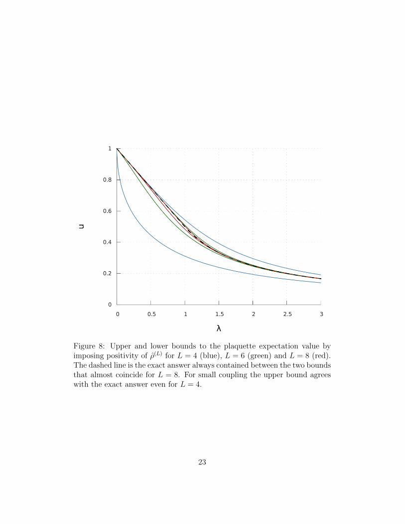
Figure 8: Upper and lower bounds to the plaquette expectation value byimposing positivity of ρ(L) for L = 4 (blue), L = 6 (green) and L = 8 (red).The dashed line is the exact answer always contained between the two boundsthat almost coincide for L = 8. For small coupling the upper bound agreeswith the exact answer even for L = 4.

23

Figure 9: For L = 4 the bounds are wide apart. However we get a goodapproximation (black curve) to the exact answer (red curve) using an effectiveaction S = −u+ 1

2λTrρ(L) ln ρ(L)

24

vanishing term gives:

det ρ(3) = 8

(w1 −

1

2

)λ2 +O(λ3) ≥ 0 ⇒ w1 ≥

1

2(3.32)

det ρ(6) = −8

(w1 −

1

2

)3

(2λ)10 +O(λ11) ≥ 0 ⇒ w1 ≤1

2,(3.33)

which then implies w1 = 12

as we know from the exact result. Higher ordersshould vanish as can be obtained by considering larger values of L. It isabsolutely clear then that a systematic expansion in λ for small coupling canonly be achieved by using the ρ matrices. The loop equation alone is notenough to fix this expansion.

3.7 Approximation

Although the results are excellent already for small values of L we can con-sider a relatively low value, e.g. L = 4 and wonder if it is possible findan approximate value of u between the maximum and the minimum. Thiswould be an approximation as opposed to the bounds that are analyticalbounds. The low coupling phase is a low temperature and therefore shouldminimize the energy, equivalently maximize u. So, at small coupling wechoose u = umax which indeed gives a very good answer, see fig.8. The largecoupling or large temperature phase should have large entropy. In this casethere is a simple entropy we can consider, namely the entropy associated tothe matrix ρ(L). Indeed, in the limit λ → 0, all loops are given by Wn = 1,ρ

(L)M has one eigenvalue equal to one and all the others vanish. Namely it

describes a pure state. Up to gauge transformations, the matrix U is theidentity and we do not lose any information if we trace its powers. On theother hand when λ → ∞ all loops vanish except W0 = 1. The matrix ρ isproportional to the identity and the entropy is a maximum. Namely, if wetake traces of powers of U we lose a maximum amount of information forthese configurations.

Therefore, the simple proposal is to maximize u for small coupling andmaximize SWL at large coupling. The results agrees with the exact solutionbetter than the bounds. An even better result is obtained by defining aneffective free energy

A = −u+ cλTrρ(L) ln ρ(L) , (3.34)

25

where c is an adjustable constant of order one. We set c = 12

because it seemsto adjust the exact answer well (see fig.9) but we do not have a way to fixthis constant from first principles. Of course the correct effective action isthe one we gave in section 3.2 but here we wanted to find a simple effectiveaction that could be used also in higher dimensions.

3.8 Summary

To summarize, what we learned from the simple two dimensional case is:There is an infinite number of solutions to the loop equation but they arerestricted by imposing positivity of ρ(L). Such condition also allows thederivation of bounds independently of the action. Once the loop equationis imposed we can derive a weak coupling expansion, strict bounds on theenergy and a simple approximation when considering short loops.

4 Four dimensional lattice

In four dimensions the numerical methods are similar as in two dimensions,the main difficulty being that the number of Wilson loops grows exponen-tially with the length. To handle that, we developed a computer programthat listed all loops up to translations, rotations, reflections and cyclic permu-tations of the links up to length L = 18 although most calculations describedbelow were done using loops up to length L = 14. It also computes thecorresponding loop equations, strong coupling expansion, and a set of ρ ma-trices that have to be positive definite as explained below. Finally it providesoutput that can be further manipulated by computer algebra programs orstandard packages such as cvx [25] or sdpa [26]. Let us now briefly describedifferent methods that can be used to solve the loop equation in differentregimes and their usefulness.

4.1 Strong coupling methods

4.1.1 Strong coupling expansion for plaquette expectation value

The strong coupling expansion for the Wilson loop can be done straight-forwardly using the loop equation [5]. Indeed writing the loop equation as

Wi =1

2λδi1 −

1

2λKi→jWj − Ci→jkWjWk , (4.1)

26

we obtain a simple solution as a series expansion

Wi =∞∑`=1

1

λ`W(`)

i , (4.2)

where

W(1)i =

1

2δi1 (4.3)

W(`)i = −1

2Ki→jW(`−1)

j − Ci→jk

`−1∑`′=1

W(`′)j W

(`−`′)k . (4.4)

We obtain the expansion for the plaquette as

u =1

2λ+

1

8λ5+O(λ−6) . (4.5)

Up to the computed order, the result agrees with eq.(2.5) thus providinga way to validate our computer code. Higher order terms require going tolarger loops or using other methods such as character expansion [12].

4.1.2 Iterative strong coupling numerical solution

Instead of doing an analytical expansion we can do a simple numerical iter-ation of eq.(4.1).

W(n+1)i =

1

2λδi1 −

1

2λKi→jW(n)

j − Ci→jkW(n)j W

(n)k . (4.6)

As seen in fig.10, the results match very well the strong coupling expansionbut diverge for λ . 1.5. The reason is that, for the iterations to converge, theeigenvalues of the operator −1

2K have to have modulus less than λ. These

eigenvalues are plotted in fig.11 where one can see that indeed the largesteigenvalue is λmax ' 1.5.

4.1.3 Strong coupling solution, analytic continuation to weak cou-pling

We can find a different iteration method to solve eq.(2.23) by doing

W(n+1)i = (Ki→j + 2λδij)

−1(δj1 − Cj→kk′W(n)

k W(n)k′

). (4.7)

27

Figure 10: The results of the iterative strong coupling method are shown.Here we can see a clear improvement as loops of longer length are includedin the calculation. However, all solutions are seen to diverge at λ ∼ 1.5.

28

Clearly the iteration is ill–defined if λ is an eigenvalue of −12K. The matrix K

is not symmetric but numerically we can still diagonalize it after truncatingit by setting to zero Wilson loops larger than a certain length. For example,keeping loops up to length L = 10, we observe that the eigenvalues of −1

2K

approximately cover an interval λ ∈ [−1.5, 1.5] on the real axis plus somesporadic eigenvalues in the complex plane that are likely the result of thetruncation. We expect that in the limit of infinite length there is a cut onthe real axis. By taking complex values of λ one can find a simple analyticcontinuation of the string coupling solution to small values of |λ| away fromthe real axis. However, one can see that such analytic continuation is not thesmall coupling solution as one can actually expect on general grounds sincethe transition is first order. This method also shows that the divergences onthe real axis are due to the fact that we truncated the loops by putting thelarger ones to zero. If that were not the case we could adjust them so thatthe right hand side of eq.(4.7) does not contain the problematic eigenvectorsof −1

2K thus avoiding the divergences. The question arises of how should

one choose the higher loops. This takes us to the next method, namely wechoose them so that that matrices ρ(L) are positive definite.

4.2 Positivity constraints

We have to construct the analogue of the matrix ρ(L) in two dimensions. Theidea is very simple, take two points x1 and x2 on the lattice and a set ofopen Wilson lines C`, ` = 1 . . . L going from x1 to x2, see fig.12. Consideran arbitrary configuration of the lattice (namely of matrices Uµ associatedwith each link) and compute the matrices U (`) associated with the curves `.Given an arbitrary set of coefficients c` we define

A =∑`

c`U(`) , (4.8)

and since TrA†A ≥ 0 for any c`, and using that the average of a non-negativequantity is non-negative, we find that the matrix of Wilson loop expectationvalues

ρ``′ = 〈Tr[(U (`)

)†U (`′)

]〉 , (4.9)

is positive semi-definite for any set of open loops and any two points x1,2.This is true in the continuum and in the lattice. For the lattice case we choosedifferent pairs of points and list all possible open loops up to a certain length.

29

Figure 11: Setting to zero loops larger than L = 10, we can diagonalize theoperator −1

2K (Wilson loop Laplacian). As seen in the figure, the eigenvalues

seem to cluster on the real axis in an approximately interval λ ∈ [−1.5, 1.5]

jx

ix

l

Figure 12: A given set of open loops connecting two points in space define a

matrix of closed loop expectation values ρ``′ = Tr[(U (`)

)†U (`′)

]that has to

be positive definite, ρ � 0.

30

In this way we construct a set of matrices that have to be positive definite.Before going into the numerical procedure let us notice a few facts regardingthis matrices that are independent of the action that we use to average theWilson loops.

• If we take x1 = x2 and two loops that start and end at x1 and sharethe first link, see fig.12, we can construct the matrix

ρ =

1 Wa Wb

Wa 1 Wc

Wb Wc 1

� 0 ⇒ 0 ≤ (Wa−Wb)2 ≤ (1−Wc)(1+Wc−2WaWb) ,

(4.10)where Wc is the intersection of Wa and Wb as in the figure. In partic-ular, if a is a plaquette, c is any loop that appears in the Laplacian ofb, namely in the loop equation for b.

• Another example is a long loop a made out of two plaquettes connectedby a long path (fig.12). Cutting this loop in two as in the figure andusing the same procedure we obtain

Wa ≥ 2u2 − 1 , (4.11)

where u is the expectation value of the plaquette. This means that, ifthe expectation value of the plaquette is close to one, there are arbitrarylong loops that are also close to one.

• Finally notice that, as in 2D, if the matrix ρ has a zero eigenvalue,namely it is in the boundary of the allowed region, then for a givenset of coefficients c` in eq.(4.8) the matrix A vanishes and this in turnimplies an infinite set of linear equations for loops that contain thegiven open paths. Namely, taking an arbitrary path C0 from xj to xiwe get

〈L∑`=1

c`Tr[U0U

(`)]〉 = 0 . (4.12)

As a simple example, let us show that if the plaquette is one (u = 1)then all loops are equal to one. Indeed, take two paths that build aplaquette as in fig.13, we get the matrix

ρ =

(1 uu 1

)� 0 ⇒ |u|2 ≤ 1 , (4.13)

31

ab c

=U1 2U

a

Figure 13: Three examples of applying the positivity constraints. The reddots denote a point where an open line starts and/or ends. The first onegives (Wa −Wb)

2 ≤ (1−Wc)(1 +Wc − 2WaWb), the second Wa ≥ 2u2 − 1,where u is the plaquette, and the third one implies that if u = 1 then forall configurations the matrices U1,2 associated with the two paths are equalU1 = U2 and then all loops are equal to one.

as expected. However, if the bound is saturated, i.e. u = 1 then thematrix associated with the zero eigenvalue should vanish. Namely A =U1 − U2 = 0. Since we can use this in any loop it simply means that,for any loop, performing a move such as the one in the same figure doesnot change its expectation value. Since any loop can be reduced to apoint by such moves, then all loops are equal to one.

4.3 Bootstrap-like method

The numerical method should now be clear. We list all loop equations andextra equations we described previously and that can be handled by thecomputer resources available. Then we construct all matrices ρ that we can

32

handle and look for solutions of the loop equation that satisfy the constraintρ � 0. This gives an upper and lower bound on u. Let us first do thisanalytically for the simplest example, the loop equation for the plaquette indimension d ≥ 3. In the notation of fig.4, the equation is

2λu = 1 +W2 + 2(d− 2)W3 −W20 −W17 − 2(d− 2)W21 . (4.14)

If we want to maximize u, we set W2 =W3 = 1, their maximum values andW20 =W17 =W21 = 2u2−1 their minimum values according to the previoussubsection, eqs.(4.10) or (4.11). We then get an equation for the maximum

u2 +λ

2(d− 1)u− 1 = 0 . (4.15)

One of the roots of this equation gives the upper bound, namely

u ≤ 1

2

(− λ

2(d− 1)+

√4 +

λ2

4(d− 1)2

)= umax , (4.16)

a bound valid for the Wilson action in a cubic lattice of any dimensiond ≥ 3. For λ → ∞ we get umax ' 2(d−1)

λand for λ → 0, umax ' 1 − λ

4(d−1).

The bound has the right behavior but the coefficients are not right, as wassomewhat expected from such crude bound. This calculation is simply anillustration that there is indeed a bound that follows from positivity of ρand the loop equation. Similarly we can get a lower bound by choosingW2 =W3 = 2u2 − 1, and W20 =W17 =W21 = 1:

u ≥ 1

2

λ

2d− 3−

√4 +

(λ

2d− 3

)2 = umin . (4.17)

To go further we can use a numerical procedure that allows us to handle ρmatrices of size of order 103 × 103 and thousands of equations. The mainobstacle is that the known numerical packages (see appendix) only deal withlinear equations. The loop equation is non-linear but we can go around it byfixing a set of loops such that the equations become linear in the rest of thevariables and then exploring the available space of such loops. In this paperwe only consider the case where we fix the plaquette u, and therefore we haveto explore only a one-dimensional space thus simplifying the calculation. Inpractice we consider loops up to a given maximum length L and the actualprocedure depends on L. Let us now consider each case.

33

4.4 Linear case, Lmax = 8, 10

Since we consider Wilson loops of maximum length given by Lmax = 8, 10 wecan only impose the loop equation associated with loops up to length L = 6.Those loops do not have self intersections and therefore the loop equations arelinear. In this case we can solve the problem using semi-definite programmingin a direct way. For example using matlab and cvx [25] (see appendix) we findthe bound depicted in fig.14. We already see that the results are reasonablefor the maximum value of u at small coupling. The minimum value of u forL8,10 turns out to be umin = 0 which is a correct but rather poor bound forthe actual value of u. So, we consider now Wilson loops of larger length.

4.5 Non-linear case in one variable, Lmax = 12, 14

In this case we impose the loop equation up to length L = 10. Some of thoseloops self-intersect and we cannot use semi-definite programming directly.However, the self-intersection splits the loops into two whose total lengthis less or equal than L = 10 and therefore one of them at least has to be aplaquette. For that reason we propose a different semi–definite programmingproblem. We fix the value of u and define a new matrix ρ as

ρ(t) = ρ− tI . (4.18)

Now we maximize the value of t by allowing the loops other than the pla-quette to take arbitrary values compatible with the loop equation. Whenthe procedure finalizes, the value of t is equal to the lowest eigenvalue of ρand it is the largest lowest eigenvalue that can be found for that fixed valueof u. Thus, if tmax < 0 it is simply not possible to choose the other loopssuch that the loop equation is satisfied and the matrix ρ � 0. Therefore thisvalue of u is not allowed. In that way we can sweep the allowed values of uand determine the bounds on u and therefore on the energy. The results aredepicted in fig.14 where the matrix ρ was truncated to an 800×800 size. Thebounds are not close to each other as they were in two dimensions. At smallcoupling we minimize the energy and therefore choose the maximum value ofu. Following the ideas discussed in section 3.7 for the two dimensional case,for large coupling we should maximize the entropy of the matrix ρ. This isnot an SDP problem and therefore we do a further approximation. Considerthe value of u where tmax(u) has a maximum. One can associate such pointwith a large value of entropy since increasing the minimum eigenvalue, with

34

0

0.2

0.4

0.6

0.8

1

0 0.5 1 1.5 2 2.5 3

uSDPA Wilson Loop Data

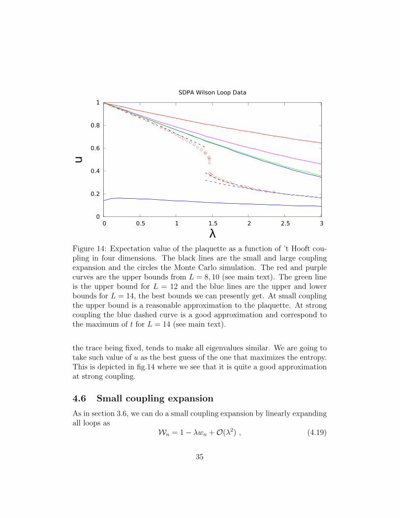
Figure 14: Expectation value of the plaquette as a function of ’t Hooft cou-pling in four dimensions. The black lines are the small and large couplingexpansion and the circles the Monte Carlo simulation. The red and purplecurves are the upper bounds from L = 8, 10 (see main text). The green lineis the upper bound for L = 12 and the blue lines are the upper and lowerbounds for L = 14, the best bounds we can presently get. At small couplingthe upper bound is a reasonable approximation to the plaquette. At strongcoupling the blue dashed curve is a good approximation and correspond tothe maximum of t for L = 14 (see main text).

the trace being fixed, tends to make all eigenvalues similar. We are going totake such value of u as the best guess of the one that maximizes the entropy.This is depicted in fig.14 where we see that it is quite a good approximationat strong coupling.

4.6 Small coupling expansion

As in section 3.6, we can do a small coupling expansion by linearly expandingall loops as

Wn = 1− λwn +O(λ2) , (4.19)

35

and finding bounds on wn. Using sdpa for loops up to length L = 12 we findfor the plaquette w1 ≥ 0.238 and for L = 14 w1 ≥ 0.2495 in agreement withthe value w1 = 1

4. Unfortunately for this length we do not find a minimum

value of u and we cannot fix w1 = 14

as we were able to do in two dimensions.

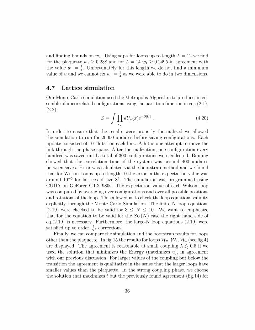
4.7 Lattice simulation

Our Monte Carlo simulation used the Metropolis Algorithm to produce an en-semble of uncorrelated configurations using the partition function in eqs.(2.1),(2.2):

Z =

∫ ∏x,µ

dUµ(x)e−S[U ] . (4.20)

In order to ensure that the results were properly thermalized we allowedthe simulation to run for 20000 updates before saving configurations. Eachupdate consisted of 10 “hits” on each link. A hit is one attempt to move thelink through the phase space. After thermalization, one configuration everyhundred was saved until a total of 300 configurations were collected. Binningshowed that the correlation time of the system was around 400 updatesbetween saves. Error was calculated via the bootstrap method and we foundthat for Wilson Loops up to length 10 the error in the expectation value wasaround 10−5 for lattices of size 84. The simulation was programmed usingCUDA on GeForce GTX 980s. The expectation value of each Wilson loopwas computed by averaging over configurations and over all possible positionsand rotations of the loop. This allowed us to check the loop equations validityexplicitly through the Monte Carlo Simulation. The finite N loop equations(2.19) were checked to be valid for 3 ≤ N ≤ 10. We want to emphasizethat for the equation to be valid for the SU(N) case the right–hand side ofeq.(2.19) is necessary. Furthermore, the large-N loop equations (2.19) weresatisfied up to order 1

N2 corrections.Finally, we can compare the simulation and the bootstrap results for loops

other than the plaquette. In fig.15 the results for loopsW2,W3,W4 (see fig.4)are displayed. The agreement is reasonable at small coupling λ . 0.5 if weused the solution that minimizes the Energy (maximizes u), in agreementwith our previous discussion. For larger values of the coupling but below thetransition the agreement is qualitative in the sense that the larger loops havesmaller values than the plaquette. In the strong coupling phase, we choosethe solution that maximizes t but the previously found agreement (fig.14) for

36

Figure 15: Expectation value of loops u = W1, W2, W3, W4 (see fig.4) aredisplayed as a function of the ’t Hooft coupling λ.

the plaquette does not extend to the other loops. Clearly, the well-knownstrong coupling expansion is still the best method in this region.

5 N = 4 SYM

The case of N = 4 SYM is particularly important since it has a dual de-scription as a string theory [1]. In the context of its relation to string theoryand more precisely with the AdS/CFT correspondence, the loop equationhas been formulated and studied in [28]. Studying the theory in the latticeshould allow a different method of computation and possible strong couplingcalculations based on the gauge theory side of the correspondence. In therest of this section we briefly describe how the ideas we developed for pure

37

YM could be implemented but, for concrete calculations, at the moment werestrict ourselves to the bosonic sector leaving the study of the full theoryfor future work.

A lattice theory that has the correct continuum theory without the needfor fine-tuning is described in [29]. Here we use that formulation but followthe notation found in the paper [30]. For brevity we do not explain detailsand refer the reader to that work for explanation of the notation and prop-erties of the theory. The main property is that such formulation preservesone twisted [31] scalar supercharge and possesses BPS Wilson loops althoughmore restricted than the continuum theory. For our purposes another im-portant property is that the action can be formulated entirely in terms ofgeneralized Wilson loops, namely using loops with fermionic links and/orsites. In this way, the form of the loop equation given in (2.22) is valid usingthe appropriate supersymmetric action [30]. However, we have not workedout the correct generalization of the ρ matrices to the fermionic sector andtherefore here we restrict ourselves to the bosonic sector described by thesimpler action

S =N

2λlat

∑x

Tr

(F †ab(x)Fab(x) +

1

2

(D(−)a Ua(x)

)2). (5.1)

This action, thought as a linear combination of Wilson loops is depicted infig.16. In order to obtain the loop equations we must vary individual links.However, the scalar and the gauge fields are twisted together which meansthat the matrices Ua(x) ∈ GL(N,C) and therefore the links and their daggersmust be treated independently:

Ua(x)⇒ (1 + iεa(x))Ua(x) (5.2)

Ua(x)⇒ Ua(x)(1− iεa(x)) . (5.3)

This implies that in eq.(2.22), the intersection of the action with the loop isnon-zero only for links oriented in the same direction, the same is true fora loop self-intersection. Since the gauge group is U(N) the ε’s do not havethe constraint that they have to be traceless simplifying the Loop Equations.The matrices ρ can be constructed similarly since we associate the hermitianconjugate of Ua to a link traversed in the opposite direction. Notice thatin this case the property that a backtracking path can be eliminated is nolonger true. In fact such backtracking paths correspond to the insertion ofscalar fields. Now we check the loop equation using a numerical simulationand leave the full exploration of the bootstrap method for future work.

38

Sm=n

-2 -2

Sm {

{N

2lS=lat

Figure 16: The Lattice action for N = 4 SYM can be written in terms ofWilson loops, the figure shows the bosonic sector that we use in the maintext. The indices µ, ν = 1 . . . 5 since the A4∗ lattice has five fundamentalvectors.

5.1 Monte Carlo Simulation

We used the parallel code developed by Schaich and DeGrand [32], basedon the previous work by Catterall and Joseph [33] to simulate the latticizedEuclidean theory. The code allows for a simple way to reduce to the bosonicsector, i.e. to the six scalars and four gauge fields that in this formulationlive on the links. The lattice is taken to be an A∗4 lattice which contains thepermutation group S5, the largest finite subgroup of the four dimensionalrotation symmetry. In order to preserve a subgroup of the SUSY Algebra,the Euclidean-Lorentz and R symmetry groups are twisted into SO(4)E ⊗SO(6)R → SO(4)′ ⊗ U(1). With this twisting the lattice theory is invariantunder one supercharge out of the full sixteen. The continuum limit shouldrestore the full sixteen supercharges without fine-tuning.

To test the loop equations we considered the loop equation associatedwith the plaquette and found that it is satisfied up to four digits which iswithin the numerical accuracy of the simulation. The test was done for U(2)and U(3) gauge groups and for λlat = 0.8, 1.0, 1.2 on 84 lattices. The resultsare presented in table 1. The loop equation necessary for the plaquette withthe pure bosonic action is given by eq. (5.4) and seen pictorial in fig. 17

1

2λlat(−W2 −W3 −W4 − 6W5 + 6W6 +W7 +W8 +W9)−W1 = 0 . (5.4)

This concludes our brief study of the N = 4 case. The next step, that weleave for future work, would be to investigate larger Wilson Loops with andwithout self-intersections and the generalization to the fermionic sector.

39

N=2 N=3

λ = 0.8 1.0 1.2 0.8 1.0 1.2

W1 0.01158 0.01451 0.01740 0.01151 0.01440 0.01724

W2 0.00241 0.00377 0.00543 0.00241 0.00377 0.00540

W3 0.00052 0.00082 0.00118 0.00048 0.00075 0.00109

W4 0.00026 0.00041 0.00059 0.00026 0.00040 0.00057

W5 0.00023 0.00036 0.00051 0.00023 0.00036 0.00051

W6 0.00205 0.00321 0.00462 0.00206 0.00321 0.00462

W7 0.00218 0.00343 0.00494 0.00219 0.00341 0.00489

W8 0.00525 0.00823 0.01184 0.00520 0.00812 0.01164

W9 0.00330 0.00518 0.00745 0.00322 0.00503 0.00723

Eq. −0.00004 −0.00004 −0.00003 0.00002 −0.000003 −0.00001

Table 1: Wilson loop expectation values used to check the loop equation(5.4)

6 Conclusions

The loop equation has been traditionally seen as a promising way to describegauge theories in terms of gauge invariant quantities. In this paper we agreewith this perspective but also point out that such equation has infinite so-lutions that have to be constrained by the condition that certain matricesare positive definite. At strong coupling such extra conditions are not neces-sary and therefore seem to have been largely ignored. On the other hand, inthe physically relevant region of small coupling such conditions are crucial toobtain the correct solution. In fact they also give many constraints and prop-erties that are actually independent of the action. In two dimensions thisleads to a simple numerical procedure that reproduces the exact solution forany coupling. This method can potentially be used for other two dimensionalactions where the exact solution is not known but, more importantly, it canbe extended to higher dimensions. The simple idea is that given two pointsin space and a set of open lines ` = 1 . . . L between them, we can define anL× L matrix of closed loops where the entry ``′ is the expectation value ofthe closed loop obtained by going along path ` and returning along path `′.

40

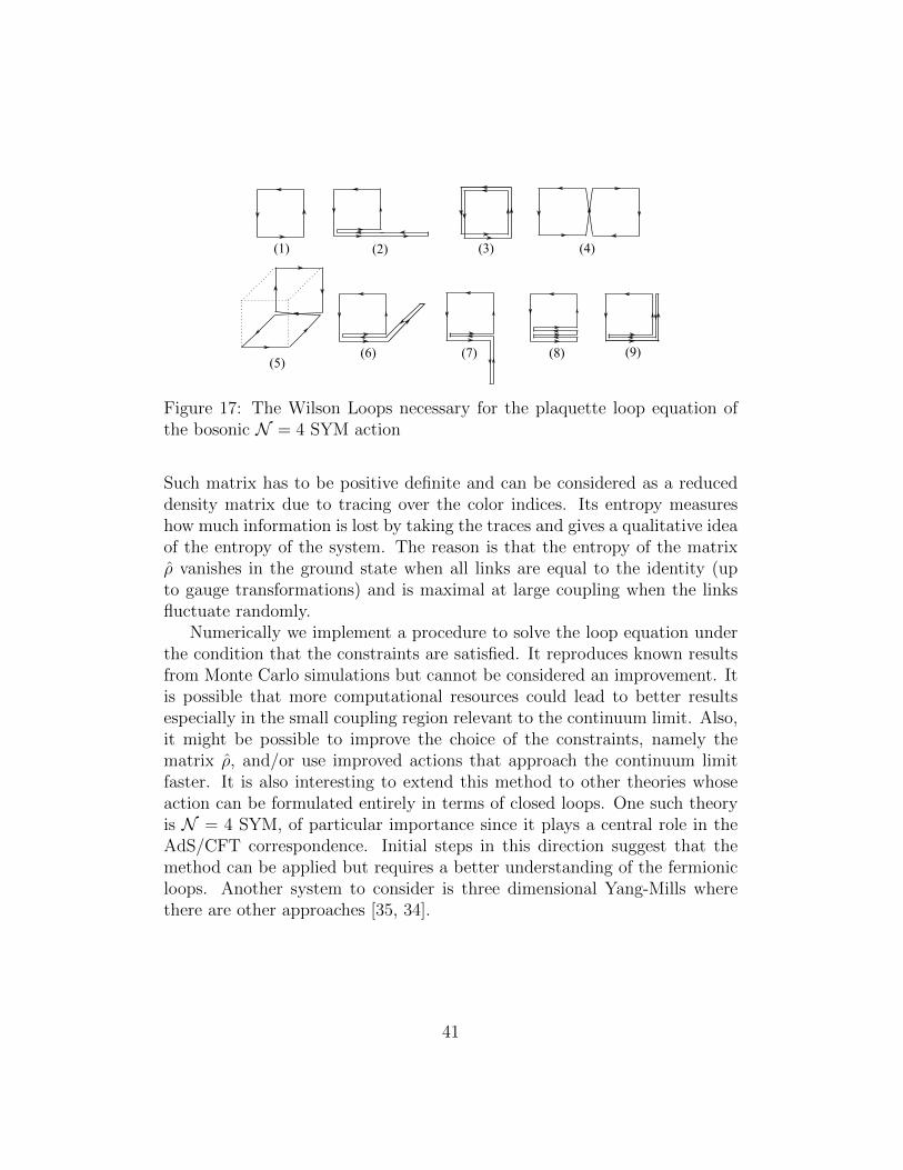
(1) (4)(3)

(5)

(2)

(6) (7) (8) (9)

Figure 17: The Wilson Loops necessary for the plaquette loop equation ofthe bosonic N = 4 SYM action

Such matrix has to be positive definite and can be considered as a reduceddensity matrix due to tracing over the color indices. Its entropy measureshow much information is lost by taking the traces and gives a qualitative ideaof the entropy of the system. The reason is that the entropy of the matrixρ vanishes in the ground state when all links are equal to the identity (upto gauge transformations) and is maximal at large coupling when the linksfluctuate randomly.

Numerically we implement a procedure to solve the loop equation underthe condition that the constraints are satisfied. It reproduces known resultsfrom Monte Carlo simulations but cannot be considered an improvement. Itis possible that more computational resources could lead to better resultsespecially in the small coupling region relevant to the continuum limit. Also,it might be possible to improve the choice of the constraints, namely thematrix ρ, and/or use improved actions that approach the continuum limitfaster. It is also interesting to extend this method to other theories whoseaction can be formulated entirely in terms of closed loops. One such theoryis N = 4 SYM, of particular importance since it plays a central role in theAdS/CFT correspondence. Initial steps in this direction suggest that themethod can be applied but requires a better understanding of the fermionicloops. Another system to consider is three dimensional Yang-Mills wherethere are other approaches [35, 34].

41

7 Acknowledgments

This work was supported in part by the DOE through grant DE-SC0007884.We are very grateful for numerous discussions with P. Vieira, S. Catterall, D.Schaich on the matters of this work and/or lattice gauge theory in general.Also S.Catterall and D. Schaich graciously provided their lattice code allow-ing us to check the loop equations in the bosonic sector of N = 4 SYM. Weare also grateful to D. Minic and A. Jevicki for useful comments on a previousversion of this work. P.D.A. would like to thank the Wigner GPU Laboratoryat the Wigner Research Center for Physics (Budapest, Hungary) for provid-ing GPUs computer resources. He would also like to thank G. G. Barnafoldi,M. F. Nagy-Egri, D. Berenyi, and Z. Bajnok for helpful discussions. M.K.wants to thank the hospitality of the Perimeter Institute, Waterloo, CA andthe SAIFR Institute (Sao Paulo, Brazil), while part of this work was beingdone.

8 Appendix: Semi-Definite programming (SDP)

Semi-definite programming [24] is a type of optimization problem that hasbeen the focus of a lot of attention recently in relation to problems in finance,engineering, and more recently has proved invaluable in the bootstrap pro-gram of conformal field theories (see e.g. [7]).

It can be stated very simply as:Given m real numbers ci=1...m ∈ R and m real, symmetric n × n ma-

trices Fi=0...m ∈ Rn×n, find xi=1...m ∈ R that minimize∑m

i=1 cixi under theconstraint that X =

∑mi=1 xiFi − F0 is positive semi-definite (X � 0).

The main observation in this field is that the space of semi-definite matri-ces is a convex cone in the space of all symmetric n×nmatrices. Indeed, giventwo positive semi-definite matrices X1,2 � 0, namely ytX1,2y ≥ 0, ∀ y ∈ Rn,then it is clear that yt(α1X1 + α2X2)y ≥ 0 for any real α1,2 ≥ 0. Thus,α1X1 + α2X2 � 0, ∀ α1,2 ≥ 0 showing that positive semi-definite matricesform a convex cone. The condition that X belongs to the linear subspacegenerated by the Fi=1...m shifted by F0 defines an intersection between thishyperplane and the semi-definite cone. This is a convex region over whichwe minimize a linear function. Therefore, the minimum is unique and shouldbe located at the boundary of the domain, namely when the matrix X has atleast one zero eigenvalue. The problem is then very similar to the more tradi-

42

tional problem of linear programming where one minimizes a linear function∑mi=1 cixi over the convex cone y`=1...n ≥ 0 where the y` =

∑mi=1 a`ixi for

some given coefficients α`i.There are many other problems that can be reduced to an SDP problem.

For example, in section 3.2 we need to solve

Minimize S = −1

λW1 +

∞∑n=1

1

nW2

n ,

such that ρ(L) =1

LT[W0, . . . ,WL] � 0 , (8.1)

this is problem of quadratic programming that can be reduced to an SDPproblem by defining a new variable t and imposing

− 1

λW1 +

∞∑n=1

1

nW2

n ≤ t , (8.2)

or equivalently

SM =

t (u− 1

2λ) W2√

2W3√

3. . .

(u− 12λ

) 1 0 0 . . .W2√

20 1 0 . . .

W3√3

0 0 1 . . ....

......

.... . .

� 0 . (8.3)

Thus the problem (8.1) is equivalent to

Minimize t, such that ρL � 0, SM � 0 . (8.4)

Once the problem has been casted as an SDP problem, there are severalavailable packages that can be used to solve it. We found that for rapid de-velopment of small problems the matlab package cvx [25] was very convenientand, for larger problems sdpa [26] was a good choice.

References

[1] J. Maldacena, “The large N limit of superconformal field theories andsupergravity,” Adv. Theor. Math. Phys. 2, 231 (1998) [Int. J. Theor.

43

Phys. 38, 1113 (1998)], hep-th/9711200,S. S. Gubser, I. R. Klebanov and A. M. Polyakov, “Gauge theory cor-relators from non-critical string theory,” Phys. Lett. B 428, 105 (1998)[arXiv:hep-th/9802109],E. Witten, “Anti-de Sitter space and holography,” Adv. Theor. Math.Phys. 2, 253 (1998) [arXiv:hep-th/9802150].

[2] G.’t Hooft, Nucl. Phys. B72 (1974) 461,G.’t Hooft, Nucl. Phys. B75 (1974) 461.

[3] Y. M. Makeenko and A. A. Migdal, “Exact Equation for the Loop Av-erage in Multicolor QCD,” Phys. Lett. 88B, 135 (1979),Y. M. Makeenko and A. A. Migdal, “Selfconsistent Areas Law In Qcd,”Phys. Lett. 97B, 253 (1980),S. R. Wadia, “On the Dyson-schwinger Equations Approach to the LargeN Limit: Model Systems and String Representation of Yang-Mills The-ory,” Phys. Rev. D 24, 970 (1981),G. F. De Angelis, D. de Falco and F. Guerra, “Lattice Gauge Models inthe Strong Coupling Regime,” Lett. Nuovo Cim. 19, 55 (1977),F. Guerra, R. Marra and G. Immirzi, “Strong Coupling Expansion forLattice Yang-Mills Fields,” Lett. Nuovo Cim. 23, 237 (1978),A.M. Polyakov, ”Gauge fields as rings of glue” Nucl. Phys. B164 (1979)171,T. Eguchi, “Strings in U(N) Lattice Gauge Theory,” Phys. Lett. 87B,91 (1979),B. Sakita, “Field Theory of Strings as a Collective Field Theory of U(N)Gauge Field,” Phys. Rev. D 21, 1067 (1980),D. Foerster, ”YangMills theory - a string theory in disguise,” Phys. Lett.87B (1979) 83,A. Jevicki and B. Sakita, “The Quantum Collective Field Method andIts Application to the Planar Limit,” Nucl. Phys. B 165, 511 (1980).

[4] A. A. Migdal, “Loop Equations and 1/N Expansion,” Phys. Rept. 102,199 (1983).

[5] G. Marchesini, “Loop Dynamics for Gauge Theories: A Numerical Al-gorithm,” Nucl. Phys. B 239, 135 (1984),G. Marchesini and E. Onofri, “Convergence Of The Iterative Solution

44

Of Loop Equations In Planar Qcd In Two-dimensions,” Nucl. Phys. B249, 225 (1985).

[6] R. Rattazzi, V. S. Rychkov, E. Tonni and A. Vichi, “Bound-ing scalar operator dimensions in 4D CFT,” JHEP 0812, 031(2008) doi:10.1088/1126-6708/2008/12/031 [arXiv:0807.0004 [hep-th]].V. S. Rychkov and A. Vichi, “Universal Constraints on Con-formal Operator Dimensions,” Phys. Rev. D 80, 045006 (2009)doi:10.1103/PhysRevD.80.045006 [arXiv:0905.2211 [hep-th]].

[7] F. Kos, D. Poland and D. Simmons-Duffin, “Bootstrapping the O(N)vector models,” JHEP 1406, 091 (2014) [arXiv:1307.6856 [hep-th]].

[8] M. F. Paulos, J. Penedones, J. Toledo, B. C. van Rees andP. Vieira, “The S-matrix Bootstrap II: Two Dimensional Amplitudes,”arXiv:1607.06110 [hep-th],M. F. Paulos, J. Penedones, J. Toledo, B. C. van Rees and P. Vieira,“The S-matrix Bootstrap I: QFT in AdS,” arXiv:1607.06109 [hep-th].

[9] A. Jevicki, O. Karim, J. P. Rodrigues and H. Levine, “Loop SpaceHamiltonians and Numerical Methods for Large N Gauge Theories,”Nucl. Phys. B 213, 169 (1983),A. Jevicki, O. Karim, J. P. Rodrigues and H. Levine, “Loop SpaceHamiltonians and Numerical Methods for Large N Gauge Theories. 2.,”Nucl. Phys. B 230, 299 (1984),A. Jevicki and B. Sakita, “Loop Space Representation and the LargeN Behavior of the One Plaquette Kogut-Susskind Hamiltonian,” Phys.Rev. D 22, 467 (1980).

[10] A. Jevicki and B. Sakita, “The Quantum Collective Field Method andIts Application to the Planar Limit,” Nucl. Phys. B 165, 511 (1980).doi:10.1016/0550-3213(80)90046-2

[11] L. G. Yaffe, “Large N Limits as Classical Mechanics,” Rev. Mod. Phys.54, 407 (1982).

[12] J. M. Drouffe and J. B. Zuber, “Strong Coupling and Mean Field Meth-ods in Lattice Gauge Theories,” Phys. Rept. 102, 1 (1983).

45

[13] Y. Makeenko, “Methods of contemporary gauge theory,” (CambridgeMonographs on Mathematical Physics), Cambridge University Press2002.

[14] M. Campostrini, “The large N phase transition of lattice SU(N) gaugetheories,” Nucl. Phys. Proc. Suppl. 73, 724 (1999)

[15] K. G. Wilson, “Confinement of Quarks,” Phys. Rev. D 10, 2445 (1974).

[16] V. A. Kazakov, “U(infinity) Lattice Gauge Theory As A Free LatticeString Theory,” Phys. Lett. 128B, 316 (1983),I. K. Kostov, “Multicolor Qcd In Terms Of Random Surfaces,” Phys.Lett. 138B, 191 (1984),I. K. Kostov, “On The Random Surface Representation Of U (infinite)Lattice Gauge Theory,” Phys. Lett. 147B, 445 (1984).

[17] U. M. Heller and F. Karsch, “One Loop Perturbative Calculation ofWilson Loops on Finite Lattices,” Nucl. Phys. B 251, 254 (1985).

[18] M. Creutz and K. J. M. Moriarty, “Phase Transition in SU(6) LatticeGauge Theory,” Phys. Rev. D 25, 1724 (1982).

[19] H. Meyer and M. Teper, “Confinement and the effective string theoryin SU(N →∞): A Lattice study,” JHEP 0412, 031 (2004)

[20] D. J. Gross and E. Witten, “Possible Third Order Phase Transition inthe Large N Lattice Gauge Theory,” Phys. Rev. D 21, 446 (1980),S. R. Wadia, “A Study of U(N) Lattice Gauge Theory in 2-dimensions,”arXiv:1212.2906 [hep-th] (unpublished 1979 EFI (U. Chicago) preprint).

[21] I.S. Gradshteyn, I.M. Ryzhik, “Table of Integrals Series and Products”,Sixth edition, Academic Press (2000), San Diego, CA, USA, London,UK.

[22] D. Friedan, “Some Nonabelian Toy Models in the Large N Limit,” Com-mun. Math. Phys. 78, 353 (1981). doi:10.1007/BF01942328

[23] Bottcher, Albrecht; Silbermann, Bernd (1990). ”Toeplitz determinants”.Analysis of Toeplitz operators. Berlin: Springer-Verlag. p. 525,See also: Toeplitz and Circulant Matrices: A Review (Foundations andTrends in Communications and Information Theory) by Robert M. Gray,Now Publishers Inc (2006).

46

[24] L. Vandenberghe and S. Boyd SIAM Review, 38(1): 49-95, March 1996.

[25] Michael Grant and Stephen Boyd. CVX: Matlab software for disciplinedconvex programming, version 2.0 beta. http://cvxr.com/cvx, Septem-ber 2013,Michael Grant and Stephen Boyd. Graph implementations for nons-mooth convex programs, Recent Advances in Learning and Control (atribute to M. Vidyasagar), V. Blondel, S. Boyd, and H. Kimura, edi-tors, pages 95-110, Lecture Notes in Control and Information Sciences,Springer, 2008. http://stanford.edu/∼boyd/graph dcp.html.

[26] ”Latest developments in the SDPA Family for solving large-scale SDPs,”Makoto Yamashita, Katsuki Fujisawa, Mituhiro Fukuda, KazuhiroKobayashi, Kazuhide Nakta, Maho Nakata, In Handbook on Semidefi-nite, Cone and Polynomial Optimization: Theory, Algorithms, Softwareand Applications , edited by Miguel F. Anjos and Jean B. Lasserre,Springer, NY, USA, Chapter 24, pp. 687–714 (2011),”A high-performance software package for semidefinite programs: SDPA7,” Makoto Yamashita, Katsuki Fujisawa, Kazuhide Nakata, MahoNakata, Mituhiro Fukuda, Kazuhiro Kobayashi, and Kazushige Goto,Research Report B-460 Dept. of Mathematical and Computing Science,Tokyo Institute of Technology, Tokyo, Japan, September, 2010,”Implementation and evaluation of SDPA 6.0 (SemiDefinite Program-ming Algorithm 6.0),” Makoto Yamashita, Katsuki Fujisawa, andMasakazu Kojima, Optimization Methods and Software 18, 491-505,2003.

[27] A. Jevicki and B. Sakita, “Collective Field Approach to the Large NLimit: Euclidean Field Theories,” Nucl. Phys. B 185, 89 (1981).

[28] A. M. Polyakov, “String theory and quark confinement,” Nucl. Phys.Proc. Suppl. 68, 1 (1998),A. M. Polyakov and V. S. Rychkov, “Gauge field strings duality and theloop equation,” Nucl. Phys. B 581, 116 (2000),A. M. Polyakov and V. S. Rychkov, “Loop dynamics and AdS / CFTcorrespondence,” Nucl. Phys. B 594, 272 (2001),N. Drukker, “A new type of loop equations,” JHEP 9911, 006 (1999)

[29] S. Catterall, D. B. Kaplan and M. Unsal, “Exact lattice supersymme-try,” Phys. Rept. 484, 71 (2009),

47

S. Catterall, D. Schaich, P. H. Damgaard, T. DeGrand and J. Giedt,“N=4 Supersymmetry on a Space-Time Lattice,” Phys. Rev. D 90, no.6, 065013 (2014),S. Catterall, “Dirac-Kahler fermions and exact lattice supersymmetry,”PoS LAT 2005, 006 (2006),D. B. Kaplan and M. Unsal, “A Euclidean lattice construction of super-symmetric Yang-Mills theories with sixteen supercharges,” JHEP 0509,042 (2005)

[30] S. Catterall, J. Giedt and A. Joseph, “Twisted supersymmetries in lat-tice N = 4 super Yang-Mills theory,” JHEP 1310, 166 (2013)

[31] N. Marcus, “The Other topological twisting of N=4 Yang-Mills,” Nucl.Phys. B 452, 331 (1995)

[32] D. Schaich and T. DeGrand, “Parallel software for lattice N=4 super-symmetric YangMills theory,” Comput. Phys. Commun. 190, 200 (2015)

[33] S. Catterall and A. Joseph, “An Object oriented code for simulatingsupersymmetric Yang-Mills theories,” Comput. Phys. Commun. 183,1336 (2012)

[34] R. G. Leigh, D. Minic and A. Yelnikov, “Solving pure QCD in 2+1dimensions,” Phys. Rev. Lett. 96, 222001 (2006),R. G. Leigh, D. Minic and A. Yelnikov, “On the spectrum of Yang-Millstheory in 2+1 dimensions, analytically,” Can. J. Phys. 85, 687 (2007).

[35] D. Karabali and V. P. Nair, A gauge-invariant Hamiltonian analysis fornon-Abelian gauge theories in (2+1) dimensions, Nucl. Phys. B 464, 135(1996),D. Karabali and V. P. Nair, On the origin of the mass gap for non-Abelian gauge theories in (2+1) dimensions, Phys. Lett. B 379, 141(1996),D. Karabali, C. j. Kim and V. P. Nair, Planar Yang-Mills theory: Hamil-tonian, regulators and mass gap, Nucl. Phys. B 524, 661 (1998),D. Karabali, C. j. Kim and V. P. Nair, On the vacuum wave functionand string tension of Yang-Mills theories in (2+1) dimensions, Phys.Lett. B 434, 103 (1998),D. Karabali, C. j. Kim and V. P. Nair, Manifest covariance and the

48

Hamiltonian approach to mass gap in (2+1)- dimensional Yang-Millstheory, Phys. Rev. D 64, 025011 (2001).

49