i

Simulation driven

pre-operative planning for the

treatment of hallux rigidus:

A novel concept of implant

assessment

Martin Paulsen

Master of Science Thesis in Medical Engineering Stockholm 2013

ii

iii

This master thesis project was performed in collaboration with

Episurf Medical AB

Supervisor at Episurf Medical AB: Nina Bake, CEO

Simulation driven pre-operative planning for the treatment of hallux rigidus: A novel concept of

implant assessment

Simuleringsdriven preoperativ planering för behandling av hallux rigidus: Ett nytt koncept

för implantatbedömning

M a r t i n P a u l s e n

Master of Science Thesis in Medical Engineering

Advanced level (second cycle), 30 credits

Supervisor at KTH: Johnson Ho

Examiner: Svein Kleiven

School of Technology and Health

TRITA-STH. 2013:98

Royal Institute of Technology

KTH STH

SE-141 86 Flemingsberg, Sweden

http://www.kth.se/sth

‘If all you ever do is all you have ever done, then all you will ever get is all you ever got.’

- Texan proverb

v

Abstract

The present study utilizes finite element analysis in order to simulate a surgical operation in the treatment of a hallux rigidus case, as designed and developed by Episurf Medical AB (Stockholm, Sweden). The surgical intervention includes an

initial cheilectomy as well as an insertion of an orthopedic implant. The goal of the study was to evaluate the current concept of the medical

intervention as it is manifested today, as well as to give design suggestions as how to further improve the pre-planning of the surgery. MRI-images of the first metatarsophalangeal joint in the hallux was collected from a patient suffering from

hallux rigidus, and used in order to build case-specific geometrical images to be used in the FE analysis. The simulation was setup as to simulate a normal motion in

the first metatarsophalangeal joint during a normal gait pattern. The first simulation was conducted without any intervention, while the second was conducted after a pre-determined operation plan in accordance with the surgical

operation that Episurf Medical AB wants to perform. The results was then compared and analyzed in order to determine the post-surgical effects that such an operation

could have on the patient. A third and final simulation was then performed, by using optimization algorithms in order to make suggestions to the pre-planned

cheilectomy shape, as well as orientation of the implant. Two parameters were being investigated in order to assess the surgical intervention as designed by Episurf Medical AB; the contact stress on the articular

side of the metatarsal head, and the strain on the implant shaft. The current manifestation of the cheilectomy did not reduce the contact stress

compared to the untreated condition, as the implant failed to be a load baring surface due to the two dimensional nature of which it is conceived. Instead, the contact surface area is reduced and positioned medial and lateral to the implant

head. The optimization algorithm could reduce the maximum contact stress significantly, from 295MPa and 400MPa in the treated and untreated conditons

respectively, to 160MPa after the optimization algorithm. It became clear that the angle of the cheilectomy as well as the orientation of the implant angle has an incriminating effect on the post-operative results. However,

the shape of the cheilectomy as well as the design of the implant would need to be revised in future embodiments, as the current concept failed to provide joint with a

new articulating surface. Further development of the models formulated in this thesis is advised, as well as validating the findings with clinical data.

vi

Abstrakt

Den aktuella studien använder finita elementmetoden i syfte att simulera en kirurgisk operation som har utvecklats av Episurf Medical AB (Stockholm, Sverige) för att behandla ett hallux rigidus fall. Det kirurgiska ingreppet utgörs av en

inledande cheilectomi, som sedan följs av att operera in ett ortopediskt implantat. Målet med studien var att utvärdera det nuvarande konceptet för det medicinska

ingrepp så som den är uttänkt idag, samt att ge designförslag för hur man ytterligare kan förbättra planeringen av operationen. MR-bilder av den första metatarsalleden i stortån samlades in från en patient som lider av hallux rigidus,

som användes sedan för att bygga patient specifika geometriska bilder för att användas i FE-analysen. Simuleringen var modellerad för att simulera en normal

rörelse i första metatarsofalangealleden under en normal gångcykel. Den första simuleringen genomfördes utan något ingripande, medan den andra genomfördes efter en förutbestämd operationsplan i enlighet med det kirurgiska

ingreppet som Episurf Medical AB vill utföra. Resultaten jämfördes sedan och analyserades för att bestämma de resultaten som en sådan operation skulle kunna

innebära för patienten postoperativt. En tredje och sista simulering utfördes sedan, med hjälp av optimeringsalgoritmer för att ge förslag på förbättringar för den

förplanerade cheilectomin, samt orienteringen av implantatet. Två parametrar undersöktes för att bedöma det kirurgiska ingrepp som designats av Episurf Medical AB, kontaktbelastningen på artikulära sidan av

metatarsalhuvudet, och påfrestningen på implantatet. Den nuvarande utformningen av cheilectomin minskade inte kontaktbelastningen

jämfört med det obehandlade tillståndet, då implantatet inte vart belastat på grund av den tvådimensionella profilen i dess utformning. Optimeringsalgoritmen kunde minska den maximala kontaktbelastningen markant, från 295MPa i den

behandlade och 400MPa i den obehandlade simuleringarna, till 160MPa efter optimeringsalgoritmen.

Det blev tydligt att vinkeln på cheilectomin samt orienteringen av implantatet har en avgörande betydelse för det postoperativa resultatet. Dock skulle formen på cheilectomin liksom designen av implantatet behöva revideras i framtida

utformningar, då det nuvarande konceptet inte lyckades att ge leden en ny ledyta. Vidareutveckling av de modeller som utvecklats i avhandlingen rekommenderas,

samt att validera resultaten med annan kliniska data.

vii

Acknowledgements

First, I would like to thank my supervisor, who has always been keen and able to swiftly help me in my work whenever in dire need, all while having been promoted to Father during the duration of the thesis; my many congratulations and my

earnest thanks. Secondly I would like to express my deepest gratitude to the good people at Episurf Medical AB, who have open heartily included me into their midst.

They have provided me with a truly inspiring environment full of laughs, knowledge and curiosity. Special thanks should be given to Nina Bake, CEO at Episurf Medical AB, for given me the opportunity to write my thesis in collaboration with the

company. It has been all I ever hoped, a fulfillment of the very reason to why I study this field of engineering. For this I´m forever grateful and I hope to keep a

close relationship with Episurf Medical AB for many years to come. I will be watching you, with hopeful and exciting eyes! I would also like to take the opportunity to express my thanks to my dear parents

Marianne and Hans Paulsen, who always eagerly give me love and support whenever needed. They have given me everything I have ever needed in order to

succeed in my education. To my dear brother Henrik Paulsen, I thank whoever is responsible for making you my brother, as there is no one greater. My very best

wishes to you and your soon-to-be wife Ellen Nordfors (whom I already regard as a dear sister!). To my other two siblings, Lina-Beth Norrström and Patrik Paulsen and their respective families; it is always a privilege to be with you and to play with all

your lovely kids. I do hope I someday will have what you two have, so that I get to treat you back for all the blessings you have given me!

To Alexandra Kidner, my dear cousin and close friend, thank you for broadening my mind with perceptions. I hope all the best to you and to your amazing boyfriend in the Philippines; you will be missed up here in Sweden!

I also would like to pay my regards to Henrik Eriksson, Sara Olsson, Simon Algstrand, Kristina Hansson, Nadja Rantatupa, Daniel Rimfjäll, Jonas Fast and

Malin Thomelius. You are the ones that make Stockholm so lovely! I would also like to show gratitude to Chiara Giordano and Candy Hung; two extraordinary women who I have had the privilege of welcoming to Stockholm; thank you both for all your

help and inspiration. I hope I will someday be at least half as good an engineer as any of you two!

To my good friends in Gothenburg, Carl Bremert and Joel Hake; we do not meet nearly as much as I would want to, but I´m very thankful your friendships and your encouragements to keep me going.

And last, but certainly not least, I have to thank my two good friends Stephanie Wikström and Sharareh Nazari, for all the hard work, patience and good fun over

the years during my master studies. You two have enriched my years at The Royal Institute of Technology tremendously; I will never forget our time together nor the many school projects we have endured, and prevailed!

viii

Content

1. Introduction ......................................................................................... 1

2. The first metatarsophalangeal joint ......................................................... 2

2.1 A short introduction to osteoarthritis ................................................. 4

2.2 Clinical implications of hallux rigidus .................................................. 4

2.3 Treatments..................................................................................... 5

2.3.1 Conservative treatments ............................................................ 6

2.3.2 Keller Resection Arthroplasty ...................................................... 7

2.3.3 Osteotomy ................................................................................ 7

2.3.4 Cheilectomy .............................................................................. 7

2.3.5 Valenti Method .......................................................................... 8

2.3.6 Arthrodesis ............................................................................... 8

2.3.7 Hemiarthroplasty ....................................................................... 9

3. Biomechanical properties ..................................................................... 10

3.1 Cartilage structure and behavior ..................................................... 11

3.1.1 Viscoelastic behavior ................................................................ 13

3.1.2 Compressive behavior .............................................................. 13

3.1.3 Tensile behavior ...................................................................... 13

3.1.4 Biphasic model ........................................................................ 14

3.1.5 Strain-dependent permeability model ......................................... 15

3.2 Bone structure and behavior ........................................................... 16

3.2.1 Cortical bone ........................................................................... 18

3.2.2 Trabecular bone ...................................................................... 19

4. Implant design ................................................................................... 21

4.1 Implant Material ........................................................................... 22

5. Materials and methods ........................................................................ 24

5.1 Geometry ..................................................................................... 25

5.2 Meshing and element type .............................................................. 26

5.3 Material properties ........................................................................ 26

5.4 Boundary, initial and loading conditions ........................................... 28

5.5 Optimization algorithm .................................................................. 29

6. Results .............................................................................................. 31

7. Conclusion and design suggestions ....................................................... 32

8. Analysis and validation ........................................................................ 33

9. Discussion and future context............................................................... 35

10. References ...................................................................................... 37

ix

Appendix A .............................................................................................. 41

1

1. Introduction

Hallux rigidus is the second most common form of disability in the first metatarsophalangeal (MTP) joint, where the most prominent and perhaps more

renown disease is hallux valgus (1). Davis-Colley was the first to describe the disease in 1887 as a “flexed plantar position of the proximal phalanx of the hallux

relative to the metatarsal head” (1; 2). He first named the disease hallux flexus, but has since then been given a multitude of names over the years; hallux rigidus, hallux limitus, dorsal bunion, hallux dolorosus and hallux malleus (1).

Hallux rigidus is the manifestation of osteoarthritis in the first MTP joint, and is a common disease with an incidence of 2.5% in people older than 50 years of age

(3). The typical age for surgical intervention in patients with hallux rigidus is between 50 and 60 years, and has a slightly higher presence in females (2; 4).

Most cases of hallux rigidus are present bilaterally, although cases have been found to be unilateral especially when correlated with some trauma or injury (1; 4). However, 80% of patients who have been monitored for a prolonged period of time

develop bilateral symptoms. In addition, about 95% of cases with a positive family history of a hallux pathology present bilateral hallux rigidus, and 80% of patients

with hallux rigidus have a positive family history. This might be because the shapes of the metatarsophalangeal joint can in itself produce stiffness in the joint, as a congenitally flat, square or chevron-shaped metatarsal head will influence the

movement in the joint (1). Many different surgical interventions can be found in the literature, advisable at

different severity levels. There are some purely conservative treatments (rest, anti-inflammatory drugs, insoles etc.) in the earlier stages of the progression, although most treatments are eminently surgical. The surgical interventions range

from osteotomies (early stages), arthrodesis (late stages) or other means of arthroplasty. (1).

A relatively new kind of operation technique has been suggested, where a defect-sized biocompatible metallic articular resurfacing implant can be used to resurface the metatarsal head with minimal invasion to the MTP joint soft tissues

(5). Carpenter et al (2010) performed a follow-up of 32 such implant resurfacing implants using the HemiCAP system (Arthrosurface Inc, Franklin, MA, USA) after a

mean period of 27.3 months and showed excellent results. A new aspiring implant design has been developed by Episurf Medical AB (Stockholm, Sweden), called the Episealer Toe. The Episealer Toe is a

cobalt-chrome based implant, with a plasma-sprayed layer of hydroxyapatite onto a layer of titanium oxide on its bone integrating pin side, and a custom made

patient specific topography on its articulating surface. The operation methodology is performed using a step-by-step methodology; the first step is to perform a cheilectomy, and the second is to drill into the intended position of the implant, and

lastly inserting the implant in its place. Both the cheilectomy and insertion positioning is determined pre-operatively, and safeguarded using custom made

guides for each patient. The aim of this study was to investigate how well the current concept can reduce the stress in the articular contact during a normal gait pattern compared to an

untreated MTP joint by performing the surgical operation in a virtual environment. The second aim of the study was to investigate how the angle of the cheilectomy

and orientation of the implant can improve the design and functionality of the implant by a simulation driven product development.

2

2. The first metatarsophalangeal joint

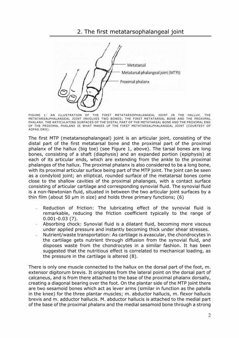
FIGURE 1: AN ILLUSTRATION OF THE FIRST METATARSOPHALANGEAL JOINT IN THE HALLUX. THE

METATARSALPHALANGEAL JOINT INVOLVES TWO BONES; THE FIRST METATARSAL BONE AND THE PROXIMAL

PHALANX. THE ARTICULATING SURFACES OF THE DISTAL PART OF THE METATARSAL BONE AND THE PROXIMAL END

OF THE PROXIMAL PHALANX IS WHAT MAKES UP THE FIRST METATARSALPHALANGEAL JOINT (COURTESY OF

AOFAS.ORG).

The first MTP (metatarsophalangeal) joint is an articular joint, consisting of the distal part of the first metatarsal bone and the proximal part of the proximal phalanx of the hallux (big toe) (see Figure 1, above). The tarsal bones are long

bones, consisting of a shaft (diaphysis) and an expanded portion (epiphysis) at each of its articular ends, which are extending from the ankle to the proximal

phalanges of the hallux. The proximal phalanx is also considered to be a long bone, with its proximal articular surface being part of the MTP joint. The joint can be seen as a condyloid joint; an elliptical, rounded surface of the metatarsal bones come

close to the shallow cavities of the proximal phalanges, with a contact surface consisting of articular cartilage and corresponding synovial fluid. The synovial fluid

is a non-Newtonian fluid, situated in between the two articular joint surfaces by a thin film (about 50 µm in size) and holds three primary functions; (6)

- Reduction of friction: The lubricating effect of the synovial fluid is

remarkable, reducing the friction coefficient typically to the range of

0.001-0.03 (7). - Absorbing chock: Synovial fluid is a dilatant fluid, becoming more viscous

under applied pressure and instantly becoming thick under shear stresses. - Nutrient/waste transportation: As cartilage is avascular, the chondrocytes in

the cartilage gets nutrient through diffusion from the synovial fluid, and

disposes waste from the chondrocytes in a similar fashion. It has been suggested that the nutritious effect is correlated to mechanical loading, as

the pressure in the cartilage is altered (8). There is only one muscle connected to the hallux on the dorsal part of the foot, m.

extensor digitorum brevis. It originates from the lateral point on the dorsal part of calcaneus, and is from there attached to the base of the proximal phalanx dorsally,

creating a diagonal bearing over the foot. On the plantar side of the MTP joint there are two sesamoid bones which act as lever arms (similar in function as the patella in the knee) for the three plantar muscles; m. abductor hallucis, m. flexor hallucis

brevis and m. adductor hallucis. M. abductor hallucis is attached to the medial part of the base of the proximal phalanx and the medial sesamoid bone through a strong

3

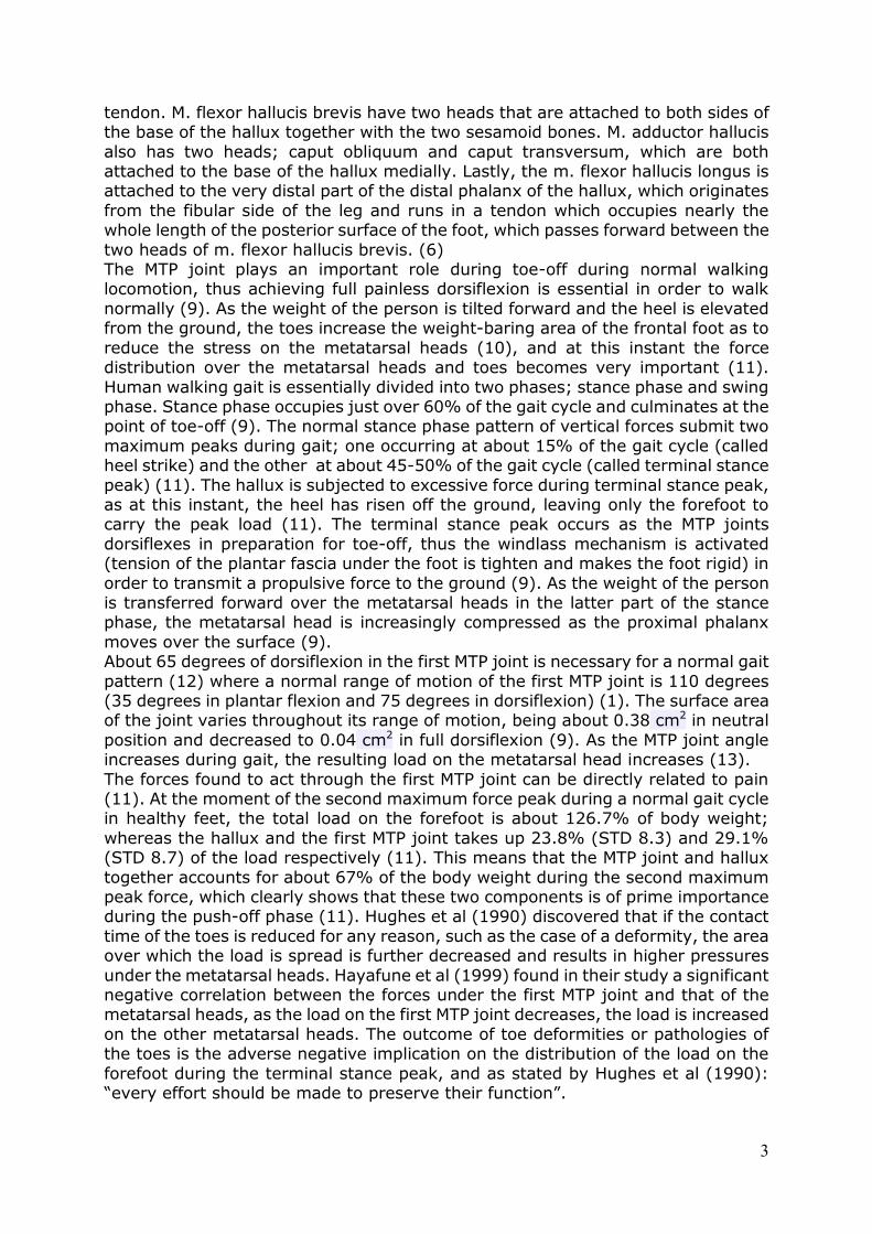
tendon. M. flexor hallucis brevis have two heads that are attached to both sides of the base of the hallux together with the two sesamoid bones. M. adductor hallucis

also has two heads; caput obliquum and caput transversum, which are both attached to the base of the hallux medially. Lastly, the m. flexor hallucis longus is attached to the very distal part of the distal phalanx of the hallux, which originates

from the fibular side of the leg and runs in a tendon which occupies nearly the whole length of the posterior surface of the foot, which passes forward between the

two heads of m. flexor hallucis brevis. (6) The MTP joint plays an important role during toe-off during normal walking locomotion, thus achieving full painless dorsiflexion is essential in order to walk

normally (9). As the weight of the person is tilted forward and the heel is elevated from the ground, the toes increase the weight-baring area of the frontal foot as to

reduce the stress on the metatarsal heads (10), and at this instant the force distribution over the metatarsal heads and toes becomes very important (11).

Human walking gait is essentially divided into two phases; stance phase and swing phase. Stance phase occupies just over 60% of the gait cycle and culminates at the point of toe-off (9). The normal stance phase pattern of vertical forces submit two

maximum peaks during gait; one occurring at about 15% of the gait cycle (called heel strike) and the other at about 45-50% of the gait cycle (called terminal stance

peak) (11). The hallux is subjected to excessive force during terminal stance peak, as at this instant, the heel has risen off the ground, leaving only the forefoot to carry the peak load (11). The terminal stance peak occurs as the MTP joints

dorsiflexes in preparation for toe-off, thus the windlass mechanism is activated (tension of the plantar fascia under the foot is tighten and makes the foot rigid) in

order to transmit a propulsive force to the ground (9). As the weight of the person is transferred forward over the metatarsal heads in the latter part of the stance phase, the metatarsal head is increasingly compressed as the proximal phalanx

moves over the surface (9). About 65 degrees of dorsiflexion in the first MTP joint is necessary for a normal gait

pattern (12) where a normal range of motion of the first MTP joint is 110 degrees (35 degrees in plantar flexion and 75 degrees in dorsiflexion) (1). The surface area of the joint varies throughout its range of motion, being about 0.38 cm2 in neutral

position and decreased to 0.04 cm2 in full dorsiflexion (9). As the MTP joint angle increases during gait, the resulting load on the metatarsal head increases (13).

The forces found to act through the first MTP joint can be directly related to pain (11). At the moment of the second maximum force peak during a normal gait cycle in healthy feet, the total load on the forefoot is about 126.7% of body weight;

whereas the hallux and the first MTP joint takes up 23.8% (STD 8.3) and 29.1% (STD 8.7) of the load respectively (11). This means that the MTP joint and hallux

together accounts for about 67% of the body weight during the second maximum peak force, which clearly shows that these two components is of prime importance during the push-off phase (11). Hughes et al (1990) discovered that if the contact

time of the toes is reduced for any reason, such as the case of a deformity, the area over which the load is spread is further decreased and results in higher pressures

under the metatarsal heads. Hayafune et al (1999) found in their study a significant negative correlation between the forces under the first MTP joint and that of the metatarsal heads, as the load on the first MTP joint decreases, the load is increased

on the other metatarsal heads. The outcome of toe deformities or pathologies of the toes is the adverse negative implication on the distribution of the load on the

forefoot during the terminal stance peak, and as stated by Hughes et al (1990): “every effort should be made to preserve their function”.

4

2.1 A short introduction to osteoarthritis

Osteoarthritis has some clear biomechanical influence on a joint’s function, since the loss of cartilage and synovial fluid will increase the friction in the joint (14).

The osteoarthritis morphology in the joint starts off in the intra cellular substance, which leads to a loss of elasticity and mass of the collagen tissue (which is quite

apparent in x-ray imaging) (14). It has been found in osteoarthritis human cartilage that the water content is above normal, which leads to a reduced compressive equilibrium modulus (see chapter 3.1.2 Compressive behavior,

nedan) (8). This means that the bone will be subjected to increased stress as the damping effect of the viscoelastic collagen rich cartilage disappears, which in turn

leads to bone deformations and increased bone density (sclerosis) (14). At the same time both the synovial membrane as well as the fibrous encapsulation around the joint will get thicker, and bony projections will form around the joint margins

(osteophyte) (14; 3), which are also quite apparent in x-ray images and often used as a clinical parameter when evaluating radiographic images of hallux rigidus

occurrence (1; 14). The biomechanical stresses that triggers the degenerative phase can be produced by a number of causes, such as; genu varum, genu valgum, injury, repetitive

motions, obesity, workload and occupation, to name a few (4). It is proposed that the degenerative morphology that changes the articular cartilage is accompanied

by an increase in subchondral bone density contributed primarily by cortical bone (15). The increased subchondral bone thickness may be the initial step in developing osteoarthritis, as stiffer subchondral bone is less capable of absorbing

forces and will transmit greater forces to the overlaying articular cartilage; thus resulting in breakdown of the cartilage matrix with ensuing synthetic and derivative

responses from the chondrocytes inside the cartilage (15). Once the degenerative phase has started, the disease will only get progressively worsen as it is a cumulative syndrome (14).

2.2 Clinical implications of hallux rigidus

People suffering from hallux rigidus suffers from a reduction in total range of motion in the MTP join, primarily in dorsal flexion with a relatively normal plantar flexion. A healthy first metatarsal head will under normal conditions serve as the

center of rotation throughout the whole motion during dorsiflexion, whereas in hallux rigidus cases the center of rotation will be located lateral to the metatarsal

head eccentrically (1). Due to this abnormal loading condition, the proximal part of the phalanx will progressively move in a plantar direction relative to the metatarsal head, which will

dorsally clamp the joint during dorsal flexion of the hallux. In such position, the hallux will be exposed to high stresses in the dorsal portion of the MTP joint, which

will give rise to cartilage lesions, and the progressive development of osteophytes and thus hallux rigidus (1). First symptoms of hallux rigidus is initially the discovery of pain localized around

the MTP joint during gait, usually during the heel lifting and/or toe-off phase (1; 4; 3). The stiffness of the joint causes pain when stressed, so patients compensates

the lack of dorsiflexion during gait by utilizing one of five typical tactics; delaying the heel lift, doing a vertical toe-off, inverting their step to toe-off using the lesser toes, performing an abductory or adductory rotation during toe-off or by flexing the

5

trunk of the body. Out if these five typical tactics, inverting the step seems to be the most frequent, followed by the delayed heel lift (4).

Other early clinical symptoms are joint swelling, decreased dorsiflexion in the MTP joint and a feeling of creaking in the joint when mobilizing the hallux (1; 4). In order to give deeper assessment and to make judgment on the proper

treatment, radio graphical examinations of the foot have to be done (1). This is usually carried out using simple 2D x-ray images taken dorsally and from a medial

or lateral view of the hallux (1). The possible causes of hallux rigidus are diverse and somewhat conflicting in the literature, but commonly reported reasons are; trauma or local injury, spontaneous

onset, ankle equinus, pes planus and functional hallux limitus (1; 4). The pain associated with hallux rigidus is believed to be secondary to the increased shear

forces at the cartilage lesion and the jamming of dorsal osteophytes upon dorsiflexion (2). Other inflammatory diseases such as rheumatoid arthritis,

seronegative arthritis, metabolic diseases (such as gouty arthritis) can also play a part in the progression of hallux rigidus (1).

2.3 Treatments

There are numerous types of treatments for hallux rigidus; the following is a draft which will explain the most common treatments in use today. Beeson et al (2008)

states in his study that there is no unifying classification system in place that is acknowledged and recognized to evaluate the severity for hallux rigidus. He and his

research team found no less than 18 different systems, and none of these had any clear credibility as they seem to rely on clinical experience rather than empirical data and without proper reliability or validity (16).

One of these classification systems is the Coughlin and Shurnas radiological classification of hallux rigidus (see Table 1) which will be used in this paper for

reference for the severity of hallux rigidus. It is considered to be a more versatile classification system, since it takes to account clinical parameters, radio graphical

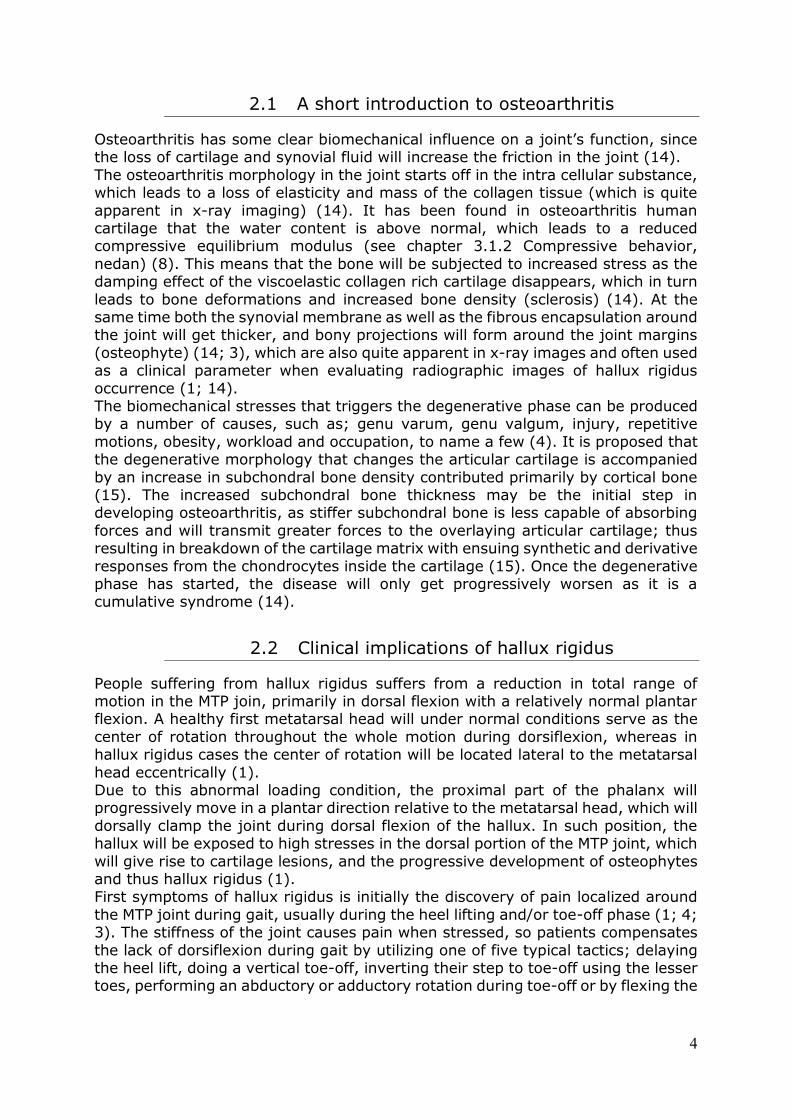
parameters as well as subjective assessments (16). TABLE 1: COUGLIN AND SHURNAS RADIOLOGICAL CLASSIFICATION OF HALLUX RIGIDUS

Stage 0 Dorsiflexion of 40-60 degrees

Normal radiography

No pain Stage 1 Dorsiflexion 30-40 degrees

Dorsal osteophytes

Minimal/ no other joint changes Stage 2 Dorsiflexion 10-30 degrees

Mild to moderate joint narrowing or sclerosis Stage 3 Dorsiflexion less than 10 degrees

Severe radiographic changes

Constant moderate to severe pain at extremities Stage 4 Stiff joint

Severe changes with loose bodies and osteochondritis dissecans

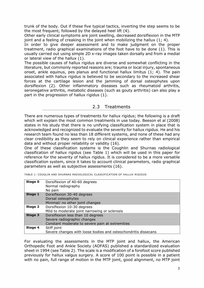
For evaluating the assessments in the MTP joint and hallux, the American

Orthopedic Foot and Ankle Society (AOFAS) published a standardized evaluation sheet in 1994 (see Table 2). The scale is a modification of a forefoot score published

previously for hallux valgus surgery. A score of 100 point is possible in a patient with no pain, full range of motion in the MTP joint, good alignment, no MTP joint

6

instability, no limitation in daily or recreational activities and with no footwear limitations. Out of the total 100 point, 45 points are appointed to function, 40 point

to pain, and 15 points to alignment in the joint (17).

TABLE 2: AMERICAN ORTHOPEDIC FOOT AND ANKLE SOCIETY’S HALLUX METATARSOPHALANGEAL-

INTERPHALANGEAL SCALE

Pain (40) -None 40

-Mild, Moderate 30

-Moderate, Daily 20

-Severe, almost always present 0

Function (45)

Activity limitations -No limitations 10

-No limitation of daily activities, such as employment responsibilities, limitation

of recreational activities

7

-Limited daily and recreational activities 4

-Severe limitation of daily and recreational activities 0

Footwear requirements -Fashionable, conventional shoes, no insert required 10

-Comfort footwear, shoe insert 5

-Modified shoes or brace 0

MTP joint motion (dorsiflexion plus plantarflexion) -Normal or mild restriction (75° or more) 10

-Moderate restriction (30°-74°) 5

-Severe restriction (less than 10°) 0

IP joint motion (plantarflexion) -No restriction 5

-Severe restriction (less than 10°) 0

MTP-IP stability -Stable 5

-Definitely unstable or able to dislocate 0

-Callus related to hallux MTP-IP 5

-Callus, symptomatic 0

Alignment (15) -Good, hallux well aligned 15

-Fair, some degree of hallux malalignment observed, no symptoms 8

-Poor, obvious symptomatic malalignment 0

2.3.1 CONSERVATIVE TREATMENTS

For patient in the early stages of hallux rigidus (see Table 1), conservative treatments might be well enough to relieve the person of pain and postpone the

almost inevitable surgical intervention. These treatments include; rest, anti-inflammatory drugs and other treatments of infected hygroma, as well as the use of insoles which slightly elevates the hallux. The use of intra articular

corticosteroid injections can improve the symptoms for the patient (1; 3).

7

2.3.2 KELLER RESECTION ARTHROPLASTY

This was previously the number one surgery used for both hallux rigidus as well as hallux valgus cases. The technique involves the resection of the proximal 2/3 of the

first phalanx base. The resection has to be that vast in order to decrease the risk of producing a painful stiffness of the MTP joint which is associated with a release of sesamoid and

articular cleaning. The Keller resection arthroplasty is still a very well used technique for Stage 3 and Stage 4 cases. (1)

2.3.3 OSTEOTOMY

There are a number of different osteotomy techniques, mainly used to treat hallux limitus. By removing some bone, either in the distal part or the proximal part of the phalanx, some remodeling and repositioning of the joint can be made. One of the

more common methods is the chevron osteotomy of the metatarsal head, where a lowering of the head through the removal of some dorsal part of the bone enables

the hallux to easier slide over the joint (see Figure 2, below). The chevron is then fixed to the bone using a cannulated screw. These kinds of surgeries are commonly used to shorten the length of the foot, if the toe is too long. The procedure is usually

used in Stage 1 or 2 cases. (1)

2.3.4 CHEILECTOMY

The first cheilectomy procedure was described in 1930 by Nilsonne (18). Since then

the procedure has undergone some changes, leading to the procedure used today, as described in 1959 by DuVries (18). The aim of a cheilectomy is to remodel the articular osteophytes of the metatarsal

bone as well as the phalanx, in order to increase the range of motion during dorsiflexion of the joint and decrease the contact stress, thus relieving the joint

from pain (see Figure 2, below) (1). The incision is made in a longitudinal dorsal-lateral or dorsal part of the joint, usually lateral of the extensor tendon of the hallux. A synovectomy is performed

and loose bodies removed through an oblique section, making a resection of the osteophyte as well as removing about 25% of the dorsal part of the metatarsal

head. Cheilectomy is a common surgical treatment for stage 2 and 3 hallux rigidus (1; 18).

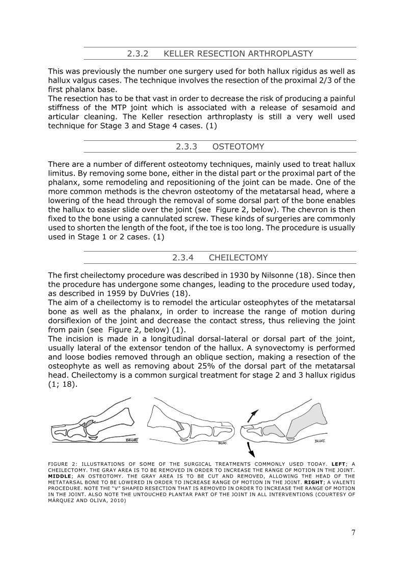
FIGURE 2: ILLUSTRATIONS OF SOME OF THE SURGICAL TREATMENTS COMMONLY USED TODAY. LEFT; A

CHEILECTOMY. THE GRAY AREA IS TO BE REMOVED IN ORDER TO INCREASE THE RANGE OF MOTION IN THE JOINT.

MIDDLE; AN OSTEOTOMY. THE GRAY AREA IS TO BE CUT AND REMOVED, ALLOWING THE HEAD OF THE

METATARSAL BONE TO BE LOWERED IN ORDER TO INCREASE RANGE OF MOTION IN THE JOINT. RIGHT; A VALENTI

PROCEDURE. NOTE THE “V” SHAPED RESECTION THAT IS REMOVED IN ORDER TO INCREASE THE RANGE OF MOTION

IN THE JOINT. ALSO NOTE THE UNTOUCHED PLANTAR PART OF THE JOINT IN ALL INTERVENTIONS (COURTESY OF

MÁRQUEZ AND OLIVA, 2010)

8

Becher, Kilger and Thermann (2005) performed a follow up of 28 patients in stage 2 and 3 hallux rigidus using a cheilectomy operative technique, and found the mean

AOFAS score to have improved from 47 preoperatively to 78 post operatively, as well as a significant decrease in pain (improvement from a mean 2.5cm preoperatively to 7.3cm postoperatively using a visual analogic scale). Their

follow-up also revealed an increase in range of motion in 23 patients (an average of 19 degrees), but also a declined range of motion in 2 patients. Significant

correlations could be found between results (subjective as well as objective) and severity stage of hallux rigidus, suggesting cheilectomy to show increasingly good results in early stages of hallux rigidus (19).

2.3.5 VALENTI METHOD

The Valenti method consists of creating a hinge design in the metaphalangeal joint. A resection of both the hallux and the metatarsal head is conducted, removing the

whole surface of the joint through an oblique angle, creating a “V” shape (see Figure 2, above). This leaves the plantar side intact, without hurting the plantar flexor muscles or the sesamoid bones (1).

This surgery is usually used for Stage 3 and Stage 4 cases (1) but has been found liable for stage 2 cases as well (20). Kurtz et al (1999) performed a follow-up on 33

patients that had underwent Valenti procedure for hallux rigidus after a mean follow-up time of 4.14 years, and could report a mean AOFAS score of 84 at time of the follow-up. 33% of the patients reported they had no pain at the time of the

follow-up, whereas 46% had mild pain, 15% had moderate pain and 0.6% had severe pain (20). 78.7% of the patients said they would undergo the same

procedure again, and 81.8% would recommend the procedure to family/friends (20).

2.3.6 ARTHRODESIS

An arthrodesis can be done in a variety of ways, but the general idea is to make the

articular surfaces fit together in order to facilitate contact between the metatarsal head and the proximal phalanx rigidly. The joint is then stabilized through a plate

(osteosynthesis) at 20 degrees dorsiflexion and 5 to 10 degrees of valgus deviation. After healing, the joint will be stiff and unable to move. (1) This surgery might be thought of as a last resort or for severe deformities of the

metaphalangeal angle, but it is commonly used in Stage 3 as well as Stage 4 hallux rigidus cases (1).

Lombardi et al (2001) performed a follow-up evaluation for 25 patients with mixed hallux rigidus stages that underwent first MTP joint arthrodesis for hallux valgus,

and found the mean AOFAS score to have been improved from 39.1 preoperatively to 75.6 postoperatively, where 8 out of 17 patients expressed 100% satisfaction with their post-operative results. Lombardi et al (2001) could not find any

significant correlation between AOFAS score and the stage of hallux rigidus (ranging from Stage 2 to 4). They did however found significant correlation

between positive AOFAS score and increased age, suggesting that elder people might demand less of their locomotive functionality thus being satisfied with pain reduction as it were (21). This theory is second by Beertema et al (2006) which

found arthrodesis procedures to results in a lower success rate compared to cheilectomy and Keller resection arthroplasty in earlier stages of hallux rigidus, but

with comparable results in agrivated stages.

9

2.3.7 HEMIARTHROPLASTY

Hemiarthroplasty refers to using an implant in order to resurface a joint surface.

This technique has been used in orthopedic applications for many years, mainly in knees and hips. The prospect of using metallic implant for treatments for hallux

rigidus has become apparent with a variety of different designs. The HemiCAP system (Arthrosurface Inc, Franklin, Massachusetts) has been prospected to be used in Stage 2 to 4 hallux rigidus cases, where a defect-sized

biocompatible metallic resurfacing implant can be used to resurface the metatarsal head with minimal invasion to the MTP joint soft tissues (5). It has of yet shown

great results, improving the mean range of motion of the MTP joint by 42 degrees (n=25) after a mean follow up of 20 months (5). Carpenter et al (2010) goes on after performing a follow-up of 32 such implant resurfacing implants using the

HemiCAP system after a mean period of 27.3 months and still showed excellent results; mean change in AOFAS from 30.8 preoperatively to 89.3 postoperatively,

whereas 94% of all cases achieved a final AOFAS score between 80 and 100, and 100% of the patients said they were satisfied with the results and would undergo

the procedure again if necessary. Carpenter et al (2010) could also report positive results in term of pain relief (4.38 preoperatively to 36.25 postoperatively) as well as increased range of motion (19.56° preoperatively to 38.28° postoperatively).

The main idea of the HemiCAP system was to minimalize the bone resection, and keep the individual anatomical geometry of the patient as much as possible (5). For

this reason, much work has been done in order to help the surgeon to locate and fix the implant by using innovative custom made tools and equipment in an engineered step-by-step methodology.

Different materials has been prospected to be used in hemiarthroplasty of the MTP joint such as metallic (cobalt-chrome based) as used by HemiCAP, or ceramic

(pyrolytic carbon) as suggested by Apard et al (2011) for Bioprofile-Tornier (Grenoble, France). They tested the designed implant in cadaveric MTP joints, and drew their conclusions based on radiological tests and fluoroscopy before and after

the insertion of their implant, thus could only validate that they had successfully been able to fixate the implant, as well as eased the movement of the hallux in the

joint (22). Roukis and Townley (2003) performed a comparative research were they compared the short-term results of a metallic resurfacing implant, called BIOPRO

(Port Huron, Michigan) to two forms of osteotomy; a Austin-Youngswick osteotomy and a Watermann-Green osteotomy. The study was conducted one year after

operation, and was shown to have similar effect in terms of range of motion, while the implant had much less incrimination to the surrounding anatomy (23). It is however quite problematic when such an articular implant fails, which forces

the surgeon to remove the implant as well as ingrown bone, creating a vast bone resection that is not easy to heal (24). In the case study reported by Hopson et al

(2009) of a failed HemiCAP implant, the implant had itself not been corrupted or fractured, but its positioning had been misaligned. The reason for this stands unknown, but could be associated with initial positioning being inadequate,

something wrong during the surgical procedure or excessive ill-positioned loads. Knessel et al (2005) investigated the reaction force under the great toe after

implantation of a TOEFIT-PLUS (Smith&Nephew, Hull, England) to understand how such an implant will affect the reaction force distribution under the hallux. They found that such an implant had a negative effect on force distribution, as 12 out of

16 patients exerted less than 50% of the reaction force found in healthy subjects under the hallux (four patients had no force apparent at all under the hallux) (25).

10

3. Biomechanical properties

Bone and cartilage are both connective tissues which are derived from

mesenchyme stem cells (26). However, they adapt quite different mechanical properties; bone is highly vascularized, cellular, and innervated whereas cartilage

tissue has low cell density, little blood supply, and no innervation (26). These material behaviors require the application of sophisticated theoretical frameworks of applied mechanics, called biomechanics (27). The presence of fluids in biological

tissues makes the tissues behave in a viscoelastic manner, giving them characteristic properties:

- Dynamic response: The bone will exert different elastic modulus depending

on loading rate; a fast loading rate will increase the elastic modulus while a

slow loading rate will decrease the reaction. - Hysteresis: The loading and unloading of stress will not follow the same

stress-strain trajectory; it takes more energy to deform thanks to the kinematic movement of fluid than when being unloaded.

- Creep: Exposure to a constant force will make the bone creep and lengthen

i.e. increased strain while under constant stress. - Stress relaxation: A constant deformation will make the bone gradually relax

i.e. decreased stress while at a fixed strain.

Connective tissues are characterized by their large amounts of extracellular

materials; mainly collagen and elastin (28). They have nonlinear anisotropic viscoelastic properties due to their composition of collagen, elastin and viscous

material, and properties as varied as the tissues themselves (28). Collagen is the main structural material of hard and soft tissues, and have a high tensile strength

(comparable to nylon: 50-100MPa) and an elastic modulus of approximately 1GPa (29; 28). Elastin serves as the elastic component in any connective tissue, with an elastic modulus of approximately 0.6MPa (29). The connective tissues are thus best

described as complex fiber-reinforced composite materials, where the extracellular collagen/elastin ratio in different connective tissues, together with any viscous or

mineral component, will give severely different material properties (29; 28). The composition and microstructure for each connective tissue is highly specialized for the particular forces for which it is subjected to e.g. a tendon has a high tensile

strength, while bone have high compressive strength (28). Both bone and cartilage are collagen rich, with complex material composition and

properties. Collagen is a macromolecule, synthesized by fibroblastic cells by linking together unique amino acid sequences. More than a dozen different types of collagen has been isolated, although the most common type is type 1 (about 90%).

However, cartilage consists mainly of type 2 collagen, characterized by its fibril shape, where it accounts for about 80% of the total collagen content. This collagen

molecule consists of three polypeptide II chains (α-chains), which are coiled in a left-handed helix with approximately 100 amino acids. These three α-chains are themselves combined in a right-handed triple helix (superhelix), giving it a length

of about 280nm and 1.5nm in diameter. Almost two-thirds of the collagen consists of three amino acids; glycine (33%), proline (15%) and hydroxyproline (15%).

Glycine enhances the stability of the molecule by forming hydrogen bonds among the three chains of the superhelix, and its repetitive sequence is essential for the proper formation of this triple-helix. Proline and hydroxyproline form hydrogen

bonded water bridges between specific groups on the chain. The chains are then

11

arranged in cross-links by covalent bonds, forming a complex matrix, giving different mechanical properties by its arrangement alone e.g. being much more

paralleled in ligaments while being tangled on the surface of the skin. (28) Collagen fibers show linear stress-strain curves, subsequent to an initial “toe” response (though to be because alignment of collagen isn’t parallel to the tensile

stress initially). Collagen has been shown to show an elastic deformation at up to 2-3% strain, while showing plasticity tendencies above approximately 4% strain.

Failure strains vary from about 11-18% strain depending on maturation. As mentioned above, the tensile strength of collagen can vary from between 50MPa to 100MPa, depending on such variables as age and anatomical location. The collagen

fibers are strain-rate dependent; tensile strength and failure strain at 720%strain/sec is approximately 108MPa and 18% respectively, compared to

61MPa and 14.7% at a strain-rate of 3.6%strain/sec. (28)

3.1 Cartilage structure and behavior

Articular cartilage is a white, dense, connective tissue, about 1-5mm thick, that covers the articular ends of the joint. The material properties of cartilage are

multiphasic, non-linearly permeable, viscoelastic, and consist of two principal components; a solid organic matrix (collagen fibrils and proteoglycan macromolecules) and a moveable interstitial fluid (predominately water with ionic

electrolytes). The largest component of the solid matrix is collagen (about 50% of the mass by dry weight), followed by proteoglycan macromolecules (about 20-30%

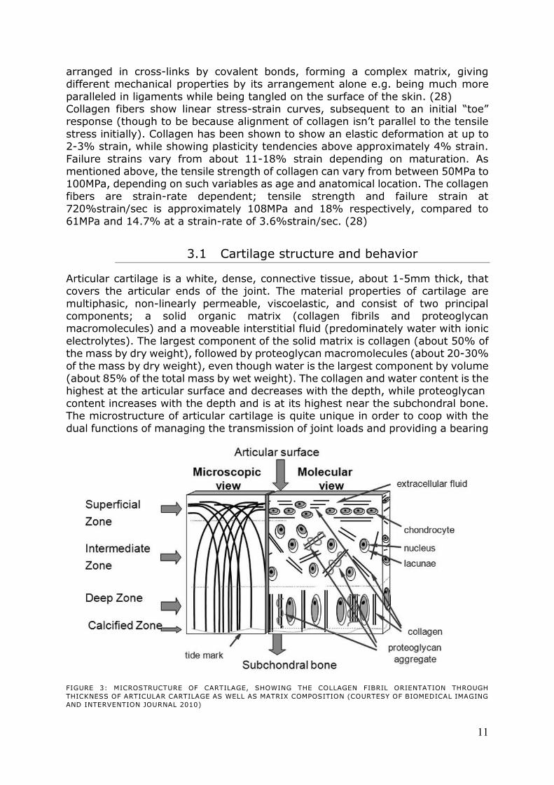
of the mass by dry weight), even though water is the largest component by volume (about 85% of the total mass by wet weight). The collagen and water content is the highest at the articular surface and decreases with the depth, while proteoglycan

content increases with the depth and is at its highest near the subchondral bone. The microstructure of articular cartilage is quite unique in order to coop with the

dual functions of managing the transmission of joint loads and providing a bearing

FIGURE 3: MICROSTRUCTURE OF CARTILAGE, SHOWING THE COLLAGEN FIBRIL ORIENTATION THROUGH

THICKNESS OF ARTICULAR CARTILAGE AS WELL AS MATRIX COMPOSITION (COURTESY OF BIOMEDICAL IMAGING

AND INTERVENTION JOURNAL 2010)

12

surface (see Figure 3, ovan). Close to the surface, collagen fibrils run parallel to the surface of the joint. Below the superficial surface, the fibril alignment becomes

progressively more oblique to the surface down to the deep zone, where collagen fibers are aligned almost perpendicular to the subchondral bone. (28) In healthy cartilage, the collagen is woven together to form a fibrous network in

which the huge proteoglycan aggregates are ‘trapped’, which together forms a cohesive porous composite organic solid matrix. The mechanical properties of

cartilage in shear and tensile strength are derived primarily from the collagen fibril properties, with the collagen-proteoglycan interaction serving a minor part. The collagen has great tensile properties (see chapter 3 Biomechanical properties,

ovan) which is useful in order to encapsulate the proteoglycans, as they have a high capacity to swell and gain or lose water when the external ionic or mechanical

environment is altered, making the proteoglycans the major contributor to the compressive resistance of the cartilage. The trapped proteoglycans contain a large

number of sulfate and carboxyl groups fixed along their glycosaminoglycan chains, which becomes negatively charged in the physiological environment and increases its osmotic pressure (30). At equilibrium, the swelling pressures from the

proteoglycans are counter-balanced by the tensile strength of the surrounding collagen matrix (called the Donnan osmatic pressure), which is the major

contributing factor for keeping the cartilage hydrated and swelled (30). Very little of the water in cartilage is intercellular, which together with the hydrophilic nature of proteoglycans and the architecture of the collagen give the tissue its

micro-porous characteristics. That means that most of the water is free to move through the tissue, and is therefore a major contributor to the mechanical

properties of cartilage, serving three primary functions: (8)

- Biological processes by augmenting the transport of nutrients into, and

waste product out of, the tissue. - Deformation processes by controlling the mechanism of the rate of fluid

transport through the deforming tissue (viscoelastic characteristics). - Providing lubrication for the thin gap between the articulating surfaces of the

joint, through exudation and imbibition caused by the deformation of the

tissue during joint articulation.

Cartilage serves as a bearing surface of articular joints as well as providing them with a low friction surface and damping effect (29). Normal, healthy cartilage exhibits remarkable wear resistant and almost frictionless performance for the joint

(µ=0.001-0.03) (8). In the extracellular matrix of collagen and proteoglycans, chondrocytes are

dispersed at low densities (the magnitude of a million cells compared to a few

hundred million cells in other tissues) (29) and is both aneural and avascular

(28). The chondrocytes are responsible for the synthesizing as well as the degradation of the organic matrix (31), but due to the avascular environment and

sparse density of the cells in the cartilage structure, cartilage has poor reconstruction capabilities (28). Adult chondrocytes grow slowly in culture, with doubling times of about 24 to 48 hours (29), and have also shown to be susceptible

to contact pressures, as chondrocytes starts to die at pressures exceeding 25MPa (28).

The biomechanical properties of articular cartilage are known to depend on exercise, age, and pathology. Immobilization of a joint has been shown to result in a loss in proteoglycans and an increased content of water; thus leading to

increased rate of creep deformation and increased permeability of joint cartilage,

13

which is paralleled to the changes observed in osteoarthritis. As the articular cartilage is softened, invading cells from the subchondral bone starts to penetrate

the cartilage, and cartilage layer is lost and replaced by bone projections (osteophyte) (see chapter 2.1 A short introduction to osteoarthritis, above). (28)

3.1.1 VISCOELASTIC BEHAVIOR

The viscoelastic effect of cartilage is contributed by the frictional drag force of

interstitial fluid (water), which flows through the porous phase, and the time-dependent deformation of the solid organic matrix. When the cartilage is

loaded, the fluid will flow out of the solid organic matrix, making it flow- and time- dependent (the fluid will not be fast enough to move if the strain-rate is too fast). At equilibrium, the fluid flow will be still, meaning the entire load on the cartilage

will be stressing the organic solid matrix. As the pressure is removed, the cartilage will resume its former configuration due to the elasticity of the organic solid matrix,

especially the increased osmotic pressure caused by the proteoglycans. (7) The fluid inside the cartilage’s ability to flow through the extracellular organic matrix of collagen and proteoglycan is governed by the pore size and the hydraulic

permeability of the extracellular matrix. Under loaded conditions, the pore size will be deformed, which will decrease the permeability in the matrix, making the

permeability of the extracellular matrix strain-dependent. (7)

3.1.2 COMPRESSIVE BEHAVIOR

The compressive modulus of cartilage is inhomogeneous; being low in the superficial layer and increases with depth towards the subchondral bone. This

effect is caused by the composition and present density of proteoglycans in the transverse layer as mention above (see chapter 3.1 Cartilage structure and

behavior). During compressive loading, the cartilage will decrease it volumetric size as the fluid begins to move within the tissue, changing the internal osmotic pressure of the proteoglycans. The effective stiffness of the cartilage is therefore

increasing with the decreased volume. (7)

3.1.3 TENSILE BEHAVIOR

The tensile modulus of cartilage is also inhomogeneous, caused by the same

mechanism as its inhomogeneous compressive modulus. However, since cartilage’s tensile strength is dependent on the collagen density, orientation and quantity; the modulus is instead at its highest at the superficial layer and decreases

with depth. When the tensile strength of cartilage is being tested, the collagen and

proteoglycan molecules are aligned with the axis of loading. The stress-strain curve for these tests shares many similarities with those done in pure collagen as they are initialized by a nonlinear toe-phase caused by the realignment of the collagen

fibrils. However, after this initial phase the stress-strain response is fairly linear and strain-dependent, in the same fashion as pure collagen. It is therefore derived that

the tensile behavior of cartilage is almost entirely due to the collagen content in the organic extracellular matrix. (7)

14

3.1.4 BIPHASIC MODEL

This basic biphasic model as described below was first described by Van C. Mow (1980) and is based on the assumptions that both the extracellular matrix and

interstitial fluid are chemically inert, that they are both incompressible, that the solid phase is ideally linearly elastic, the strains are infinitesimal, that the fluid is ideal (i.e. no viscosity), and that the inertia forces are negligible.

If the whole cartilage is denoted the volume V, then the volumetric fraction of each phase is;

EQUATION 1

where s stands for solid phase, and f stands for fluid phase. The saturation for

EQUATION 1 must therefore hold that;

EQUATION 2

The total stress acting at a point in the tissue is given by the sum of the solid and fluid stresses;

EQUATION 3

where is the effective stress tensor due to elastic deformation of the solid phase,

is the hydrostatic fluid pressure from the fluid phase, and is the unit tensor. The

effective stress tensor is given by;

EQUATION 4

where is cubic dilatation, is the strain tensor, and and are the first and

second Lamé constants respectively. and , as well as the aggregate modulus of

the solid phase , that are used in this biphasic model, are related to the elastic

modulus (Young’s modulus) and the Poisson ratio , as;

( )

( )

EQUATION 5

By assuming that each phase is incompressible, fully saturated, and that no mass is exchanged, the law of conservation of mass can be utilized;

( ( )) EQUATION 6

where and are the velocities of the solid and fluid phases respectively. The

vector ( ) gives the relative velocity of the fluid phase with respect to the

solid phase; that is the fluid flow through the surface of the extracellular matrix. According to Darcy’s law, the fluid flux is related to the hydrostatic fluid pressure,

thus;

15

( ) EQUATION 7

where k is the hydraulic permeability. The law of conservation of mass (EQUATION 6)

can together with EQUATION 7 be written as;

( ) EQUATION 8

This isotropic biphasic model has been utilized to analyze confined as well as unconfined compressions, for both normal and osteoarthritis cartilage. To this, a depth dependency of the articular cartilage can be included by a depth dependent

stiffness or permeability, as well as a fluid flow-dependent viscoelasticity. (7)

3.1.5 STRAIN-DEPENDENT PERMEABILITY MODEL

The strain-dependent permeability (caused by the deformation and volumetric change of the pore size in the solid phase) can be described as;

EQUATION 9

where and are material constants, and is the change in volume in the solid

phase. Given the void ratio ( ), this can be written as;

(

)

EQUATION 10

where and are the void ratios of current and initial scenarios, respectively. The

behavior of cartilage is however, very complex to describe in full detail. There exists today a variety of different models that can with good estimates describe

different characteristics of the mechanics of cartilage as mentioned above. (7)

16

3.2 Bone structure and behavior

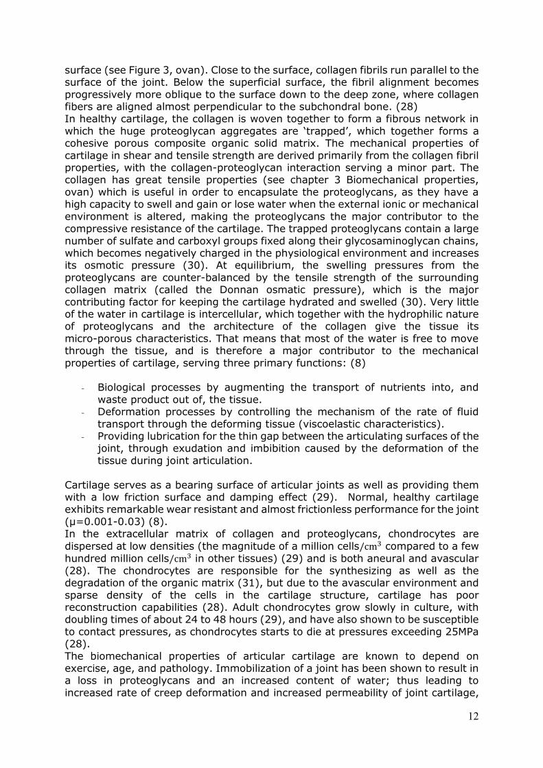
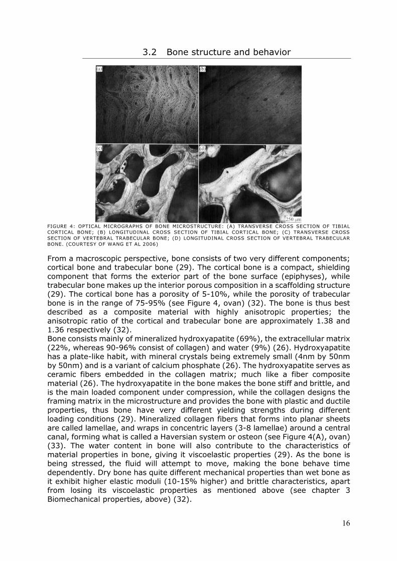
FIGURE 4: OPTICAL MICROGRAPHS OF BONE MICROSTRUCTURE: (A) TRANSVERSE CROSS SECTION OF TIBIAL

CORTICAL BONE; (B) LONGITUDINAL CROSS SECTION OF TIBIAL CORTICAL BONE; (C) TRANSVERSE CROSS

SECTION OF VERTEBRAL TRABECULAR BONE; (D) LONGITUDINAL CROSS SECTION OF VERTEBRAL TRABECULAR

BONE. (COURTESY OF WANG ET AL 2006)

From a macroscopic perspective, bone consists of two very different components; cortical bone and trabecular bone (29). The cortical bone is a compact, shielding

component that forms the exterior part of the bone surface (epiphyses), while trabecular bone makes up the interior porous composition in a scaffolding structure (29). The cortical bone has a porosity of 5-10%, while the porosity of trabecular

bone is in the range of 75-95% (see Figure 4, ovan) (32). The bone is thus best described as a composite material with highly anisotropic properties; the

anisotropic ratio of the cortical and trabecular bone are approximately 1.38 and 1.36 respectively (32). Bone consists mainly of mineralized hydroxyapatite (69%), the extracellular matrix

(22%, whereas 90-96% consist of collagen) and water (9%) (26). Hydroxyapatite has a plate-like habit, with mineral crystals being extremely small (4nm by 50nm

by 50nm) and is a variant of calcium phosphate (26). The hydroxyapatite serves as ceramic fibers embedded in the collagen matrix; much like a fiber composite

material (26). The hydroxyapatite in the bone makes the bone stiff and brittle, and is the main loaded component under compression, while the collagen designs the framing matrix in the microstructure and provides the bone with plastic and ductile

properties, thus bone have very different yielding strengths during different loading conditions (29). Mineralized collagen fibers that forms into planar sheets

are called lamellae, and wraps in concentric layers (3-8 lamellae) around a central canal, forming what is called a Haversian system or osteon (see Figure 4(A), ovan) (33). The water content in bone will also contribute to the characteristics of

material properties in bone, giving it viscoelastic properties (29). As the bone is being stressed, the fluid will attempt to move, making the bone behave time

dependently. Dry bone has quite different mechanical properties than wet bone as it exhibit higher elastic moduli (10-15% higher) and brittle characteristics, apart from losing its viscoelastic properties as mentioned above (see chapter 3

Biomechanical properties, above) (32).

17

Bone is a living and constantly remodeling material, with living cells inside its framework. Osteoclasts will constantly break down bone, while osteoblasts will

remodel new bone in accordance to the loading conditions of the bone (called Wolf’s law) (29; 15). The remodeling of bone follows the principal stress trajectories during loading, making distortions in the principal stress (which can become

evident by orthopedic implants) to have an incriminating effect on the microstructure of the bone (34).

Trabecular bone is much more active metabolically and is remodeled more often than cortical bone, which is also though to affect the material properties (33). Mechanical stress plays a major role in the regulation of skeletal development

which results in a system modified for the physical function it performs (15). Osteoporosis, for example, is a disorder in which old bone is broken down by the

osteoclast faster than the osteoblast can create new bone, making the bone degradingly weaker (29).

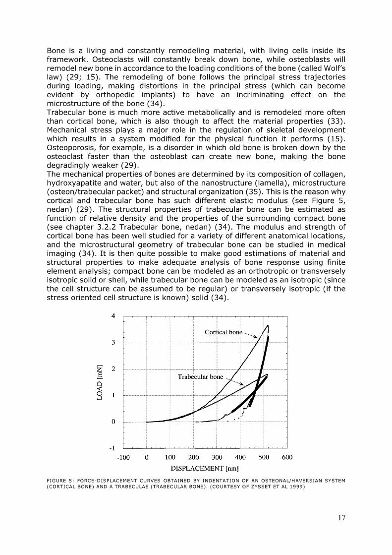
The mechanical properties of bones are determined by its composition of collagen, hydroxyapatite and water, but also of the nanostructure (lamella), microstructure (osteon/trabecular packet) and structural organization (35). This is the reason why

cortical and trabecular bone has such different elastic modulus (see Figure 5, nedan) (29). The structural properties of trabecular bone can be estimated as

function of relative density and the properties of the surrounding compact bone (see chapter 3.2.2 Trabecular bone, nedan) (34). The modulus and strength of cortical bone has been well studied for a variety of different anatomical locations,

and the microstructural geometry of trabecular bone can be studied in medical imaging (34). It is then quite possible to make good estimations of material and

structural properties to make adequate analysis of bone response using finite element analysis; compact bone can be modeled as an orthotropic or transversely isotropic solid or shell, while trabecular bone can be modeled as an isotropic (since

the cell structure can be assumed to be regular) or transversely isotropic (if the stress oriented cell structure is known) solid (34).

FIGURE 5: FORCE-DISPLACEMENT CURVES OBTAINED BY INDENTATION OF AN OSTEONAL/HAVERSIAN SYSTEM

(CORTICAL BONE) AND A TRABECULAE (TRABECULAR BONE). (COURTESY OF ZYSSET ET AL 1999)

18

3.2.1 CORTICAL BONE

Cortical bone has a porosity of 5-10%, and consists of repeating units called Haversian systems or osteons (32). The microstructure of cortical bone is

composed of regular, cylindrically shaped lamellae (33). The osteons have shown to have very different properties in tension, compression, bending and torsion; 12GPa, 6GPa, 2GPa and 20GPa respectively (33).

Because of the orthotropic nature of bone, the criteria for the prediction of onset of e.g. plastic deformation, which are based on isotropic material models (such as

Tresca or von Mises) cannot be used. However, generalizations of these have found to be adequate models for predicting of both plasticity and fracture of bone, based on the criteria used for other composite materials. (34)

von Mises yield criterion for an isotropic material for an arbitrary stress state ( ), plastic deformation starts when:

{

( )

( )

( )

}

EQUATION 11

where is the yield strength of the isotropic material. For an anisotropic material, the criterion can be generalized through the material properties F, G, H, L, M and N:

( ) ( )

( )

EQUATION 12

According to Tsai Hill, the yield strengths ( ) of a composite

material is related to the parameters F to N. By making tests of the bone in its principal directions, we can deduce the following:

- If only acts on the bone, then;

EQUATION 13

- If only acts on the bone, then;

EQUATION 14

- If only act on the bone, then;

EQUATION 15

- If only act on the bone, then;

EQUATION 16

Long bones can be treated as transversely isotropic, and can therefore be assumed

to possess the same failure strength in radial and tangential direction, e.g. .

As compact bone can be regarded as thin, we can assume a state of plane stress;

19

EQUATION 17

This will together form the Tsai-Hill failure criterion for a material in a state of plane stress:

EQUATION 18

It is very important when using this criterion to use the correct material property to

the correct axial loading; a negative σ would mean compression and a positive σ would mean tensile, using the corresponding failure criterion (34). The cortical bone properties are greatly influenced by the porosity, mineralization level and

organization of the solid extracellular matrix (collagen) (33). The mechanical properties of the microstructural level vary from one bone to another, and even at

different regions of the same bone (33).

3.2.2 TRABECULAR BONE

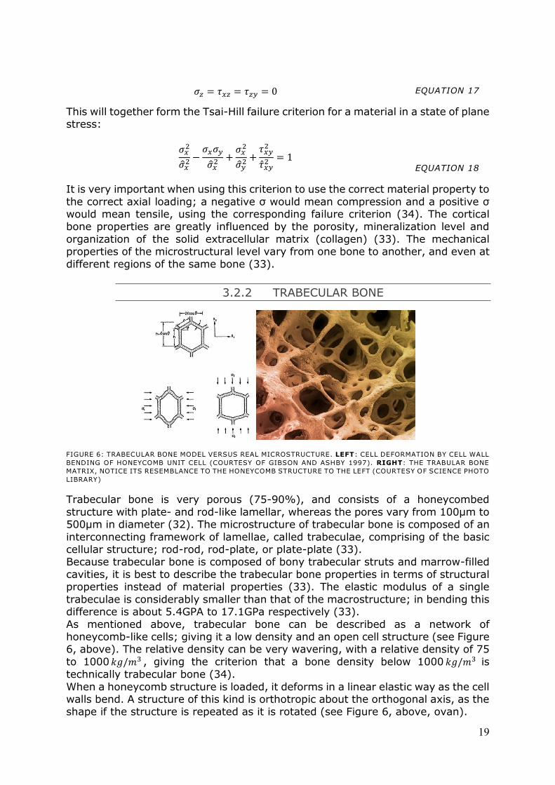
FIGURE 6: TRABECULAR BONE MODEL VERSUS REAL MICROSTRUCTURE. LEFT: CELL DEFORMATION BY CELL WALL

BENDING OF HONEYCOMB UNIT CELL (COURTESY OF GIBSON AND ASHBY 1997). RIGHT: THE TRABULAR BONE

MATRIX, NOTICE ITS RESEMBLANCE TO THE HONEYCOMB STRUCTURE TO THE LEFT (COURTESY OF SCIENCE PHOTO

LIBRARY)

Trabecular bone is very porous (75-90%), and consists of a honeycombed

structure with plate- and rod-like lamellar, whereas the pores vary from 100µm to 500µm in diameter (32). The microstructure of trabecular bone is composed of an

interconnecting framework of lamellae, called trabeculae, comprising of the basic cellular structure; rod-rod, rod-plate, or plate-plate (33). Because trabecular bone is composed of bony trabecular struts and marrow-filled

cavities, it is best to describe the trabecular bone properties in terms of structural properties instead of material properties (33). The elastic modulus of a single

trabeculae is considerably smaller than that of the macrostructure; in bending this difference is about 5.4GPA to 17.1GPa respectively (33).

As mentioned above, trabecular bone can be described as a network of honeycomb-like cells; giving it a low density and an open cell structure (see Figure 6, above). The relative density can be very wavering, with a relative density of 75

to 1000 , giving the criterion that a bone density below 1000 is

technically trabecular bone (34).

When a honeycomb structure is loaded, it deforms in a linear elastic way as the cell walls bend. A structure of this kind is orthotropic about the orthogonal axis, as the shape if the structure is repeated as it is rotated (see Figure 6, above, ovan).

20

Assuming the honeycomb has a low relative density, e.g. the cell walls to be thin, the density can be found by simple geometry:

( )

( )

EQUATION 19

Or for regular hexagon geometry where h=l and =30°:

EQUATION 20

As the structure is stressed by (see Figure 6, ovan), the cell walls will tend to

bend as caused by the bending moment:

( )

( )

EQUATION 21

This can be considered as a cantilever beam with an edge load of and

with an edge bending moment ⁄ , thus can be written as:

EQUATION 22

Where is the moment of inertia of a cell wall with uniform thickness and is the

degree of bending of the beam, as the component is parallel to the -axis (see Figure 6, above), it is possible to derive the strain in this direction:

( )

EQUATION 23

The elastic modulus (Young’s modulus) in the -axis is thus:

(

)

EQUATION 24

Similar expression of the elastic modulus can be derived in the -axis when a

stress is applied by a similar geometrical methodology, culminating in the expression:

(

)

EQUATION 25

For a regular hexagon (h=l and =30°) with cell walls of uniform thickness, both the elastic moduli

and will be reduce to the same value, resulting in a

honeycomb with quasi-isotropic properties (that is, isotropic in - and -axis) (36). The Poisson ratios will both become equal to 1 for regular hexagon cells; the

Poisson ratios are thus only dependent on the cell geometry and not the relative density of the cell (36).

21

4. Implant design

Episurf Medical AB has developed a metallic resurfacing implant to be used for

patients suffering from hallux rigidus. The concept of the implant is designed to be used in early progressions with minimal invasiveness, primarily in cases where the

patient is in a position where the functionality of the foot will heavily influence once quality of life e.g. active 40-50 year olds. The implant consists of a ‘plug’-like design in one solid construction, made in a

cobalt-chrome alloy. The entire implant except the very top of the head is then plasma-sprayed with hydroxyapatite onto an initial layer of titanium oxide, in order

to promote cell growth anchorage to the implant (osseointegration). The topography of the head of the implant is individually designed according to patient specific anatomy using MRI - or CT-segmentations. The implant is inserted as a peg

into the subchondral bone, which will save the implant from tough handling during insertion (e.g. from screw insertion).

In their first product, which is to be situated in the knee, the positioning of the implant becomes apparent simply by localizing the lesion in the cartilage from MRI-images. The insertion of the implant covers the cartilage lesion with a 0.5mm

vertical resection, making the implant head not initially load bearing against the opposing cartilage/menisci (7). In such an application, it is essential that the

implant is indeed inserted in exactly the same orientation and alignment during surgery, as the implant has been positioned and thus designed during the manufacturing process in order to make use of the individual topography of the

implant head. For this reason, each individual implant is delivered with a corresponding individual drill guide system, which is to ensure that the positioning

of the implant is correctly inserted at its intended position and orientation. A similar methodology has been suggested to be used in the advancement for an

implant to be used for the treatment of hallux rigidus cases. However, because of the distinct differences between these two joints (knee and MTP joint); the technology is not directly applicable. The MTP joint is usually heavily deformed due

to the osteophytes, which has to be removed, leaving little of the original cartilage intact. In addition, an implant situated in the MTP joint will not be subjected to

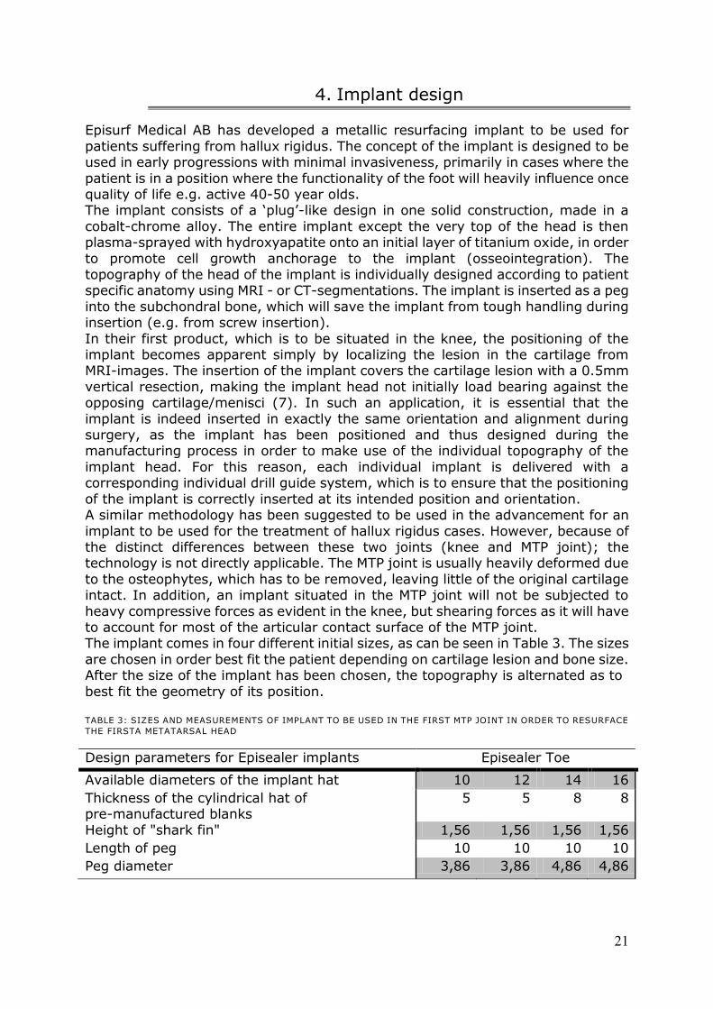
heavy compressive forces as evident in the knee, but shearing forces as it will have to account for most of the articular contact surface of the MTP joint. The implant comes in four different initial sizes, as can be seen in Table 3. The sizes

are chosen in order best fit the patient depending on cartilage lesion and bone size. After the size of the implant has been chosen, the topography is alternated as to

best fit the geometry of its position. TABLE 3: SIZES AND MEASUREMENTS OF IMPLANT TO BE USED IN THE FIRST MTP JOINT IN ORDER TO RESURFACE

THE FIRSTA METATARSAL HEAD

Design parameters for Episealer implants Episealer Toe

Available diameters of the implant hat 10 12 14 16

Thickness of the cylindrical hat of pre-manufactured blanks

5 5 8 8

Height of "shark fin" 1,56 1,56 1,56 1,56

Length of peg 10 10 10 10

Peg diameter 3,86 3,86 4,86 4,86

22

As the Episealer Toe concept is manifested as of now, the insertion will principally follow this simplified step-by-step methodology:

1. The head of the first MTP joint is exposed by the surgeon 2. A cheilectomy guide is designed and used for each individual patient,

ensuring that the bone resection of the dorsal osteophytes is as intended pre-operatively.

3. A drill guide is designed and used for each individual patient, based on the pre-determined cheilectomy.

4. The implant is inserted into its intended position, with a unique topography

that is to resurface the articular surface according to the patient specific anatomy of the intended position.

As the topography and positioning of the implant can with good estimates be tailor

made pre-operatively, only one question remains; where to put the implant in order to acquire best fidelity. The positioning of the implant should be made in order to disperse the stresses during the loading of the joint evenly across the joint,

while not risking displacement of the implant. The smaller the implant design, the more accuracy of the placement of the implant needs to be in order to provide a

functional MTP joint to the patient.

4.1 Implant Material

The implant is made of a solid piece cobalt/chromium/molybdenum alloy (ASTM F1537-08). This alloy is well used for surgical implants, especially in orthopedics. The bottom part (peg) of the implant is then coated with hydroxyapatite (ASTM

F1185) onto an interlaying titanium coating (ASTM F1580). Both of the coatings thickness is 30 +/- 10 µm, with a porosity of 4-7% in the titanium and less than

10% in the hydroxyapatite, with a combined roughness of ( value) 40-80µm. The use of hydroxyapatite coated onto an interlayer of titanium oxide has proven to

show an impressive osseointegration, in early as well as prolonged fixation. The cobalt/chromium/molybdenum alloy has been used for many years in orthopedic and dental applications mostly because of its wear and corrosion

resistance, its manufacturing features (the alloy can be well polished, with a micro-roughness of <1µm) and material properties such as high strength and

hardness modulus. The alloy has been shown to be cytotoxic, genotoxic, carcinogenic (although not proven for orthopedic applications) and shows toxicity, but has been approved by the International Agency for Research on Cancer to be

used for hip and knee prosthesis. Titanium has been used in dental application since the 1960s. The term

osseointegration was conceived by Per-Ingvar Brånemark to explain the acceptance and mechanical anchoring of titanium surfaces in contact with bone.

Osseointegration is the direct structural and functional connection between living bone and implant surface, much contributed by the porous similarity between that of titanium oxide and trabecular bone. Due to the corrosion resistant nature of

titanium dioxide, in combination with its micro-roughness, it is well used in dental implants with great results (37).

Hydroxyapatite is the major constituent of bone (69%, see chapter 3.2 Bone structure and behavior, above) (26). Because of its given biocompatibility towards bone, it has become increasingly used as an interlocking layer between that of bone

implant and bone, serving as an intermediate connective layer (37).

23

Hydroxyapatite ceramics undergo a gradual substitution with bone through an osteoconductive process, which will give rapid osseointegration and promote

osteoblast cell attachment and thus bone healing. This enhanced integration has proven to improve clinical success rates in long-term follow-ups compared to uncoated titanium dental implants, believed to be due to the superior initial rate of

osseointegration. Coating implants with hydroxyapatite does have its drawbacks; it is hard to plasma-spray on small complex shapes (such as screws) and has shown

to delaminate from the implant surface despite the fact that the coating is well-attached to the bone tissue. This is believed to be because of the brittle nature of the ceramic apatite, which is heavily strained when implanted using

screw-fixation as used in dental applications, proving to have weak material properties (38).

24

5. Materials and methods

In order to perform the evaluation of the surgical intervention prospected by

Episurf Medical AB, simulations were carried out using the finite element method (FEM). FEM is a well-used engineering numerical method as to investigate and

evaluate products early in its design phase. The method has with increased confidence been implemented as an integrate part of any design phase, as to evaluate functionality and optimize the design before prototyping the product. Its

accuracy of the calculations is directly related to which extent the scenario which is being investigated has been successfully modeled and described.

The problem at hand is very complex, posing problems in its geometry, material composition and boundary conditions in order to simulate the conditions in the first MTP joint during normal locomotion. The aim of the surgical intervention is to allow

the patient to walk without restrains in range of motion due to pain associated with the presence of hallux rigidus. For this purpose, three simulations are used; a MTP

joint suffering from hallux rigidus; a post-operative assessment of a treated MTO joint, that has undergone an virtual surgical intervention as described by Episurf Medical AB; and an suggested improvement of the surgical intervention,

formulated using optimization algorithms as to improve the outcome following the cheilectomy and orientation of the implant.

The analysis was carried out in a case study fashion; a patient suffering from hallux rigidus was operated upon in accordance with the surgical technique developed by Episurf Medical AB in a virtual environment. The post-operative results are thereby

analyzed by comparing the stresses in the articular contact surface pre- versus post-operation.

The angle of cheilectomy and the orientation of the implant were further investigated upon in order to give design suggestions as to improve the outcome of

the operation, using optimization algorithms. For this reason, two algorithms were used; one to minimize the maximum contact stress in the joint by investigating the geometrical shape of the performed cheilectomy, and one to investigate how the

orientation of the implant can lower the strains on the implant shaft. The simulations were all done in Ansys Workbench 14 (Swanson Analysis Inc.,

Huston, Pa, USA) using the static structural analysis of the mechanical APDL for structural physics. The explicit substeps were defined in time, with an allowed time-step of 0.00005 seconds per interaction.

The parameters investigated are equivalent (van Mises) stress in the contact area on the metatarsal side of the articular joint, and the strains on the implant shaft.

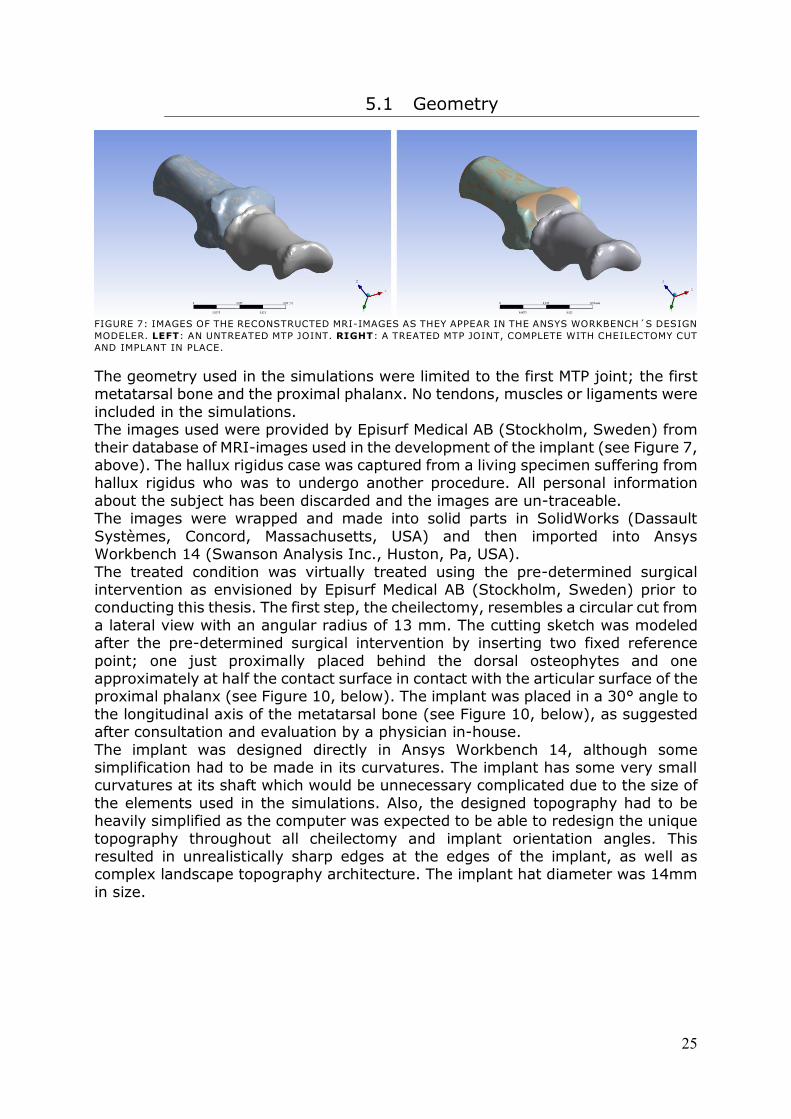
25

5.1 Geometry

FIGURE 7: IMAGES OF THE RECONSTRUCTED MRI-IMAGES AS THEY APPEAR IN THE ANSYS WORKBENCH´S DESIGN

MODELER. LEFT: AN UNTREATED MTP JOINT. RIGHT: A TREATED MTP JOINT, COMPLETE WITH CHEILECTOMY CUT

AND IMPLANT IN PLACE.

The geometry used in the simulations were limited to the first MTP joint; the first metatarsal bone and the proximal phalanx. No tendons, muscles or ligaments were

included in the simulations. The images used were provided by Episurf Medical AB (Stockholm, Sweden) from

their database of MRI-images used in the development of the implant (see Figure 7, above). The hallux rigidus case was captured from a living specimen suffering from hallux rigidus who was to undergo another procedure. All personal information

about the subject has been discarded and the images are un-traceable. The images were wrapped and made into solid parts in SolidWorks (Dassault

Systèmes, Concord, Massachusetts, USA) and then imported into Ansys Workbench 14 (Swanson Analysis Inc., Huston, Pa, USA).

The treated condition was virtually treated using the pre-determined surgical intervention as envisioned by Episurf Medical AB (Stockholm, Sweden) prior to conducting this thesis. The first step, the cheilectomy, resembles a circular cut from

a lateral view with an angular radius of 13 mm. The cutting sketch was modeled after the pre-determined surgical intervention by inserting two fixed reference

point; one just proximally placed behind the dorsal osteophytes and one approximately at half the contact surface in contact with the articular surface of the proximal phalanx (see Figure 10, below). The implant was placed in a 30° angle to

the longitudinal axis of the metatarsal bone (see Figure 10, below), as suggested after consultation and evaluation by a physician in-house.

The implant was designed directly in Ansys Workbench 14, although some simplification had to be made in its curvatures. The implant has some very small curvatures at its shaft which would be unnecessary complicated due to the size of

the elements used in the simulations. Also, the designed topography had to be heavily simplified as the computer was expected to be able to redesign the unique

topography throughout all cheilectomy and implant orientation angles. This resulted in unrealistically sharp edges at the edges of the implant, as well as complex landscape topography architecture. The implant hat diameter was 14mm

in size.

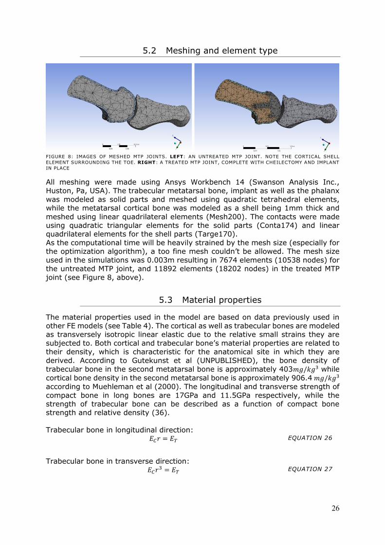
26

5.2 Meshing and element type

FIGURE 8: IMAGES OF MESHED MTP JOINTS. LEFT: AN UNTREATED MTP JOINT. NOTE THE CORTICAL SHELL

ELEMENT SURROUNDING THE TOE. RIGHT: A TREATED MTP JOINT, COMPLETE WITH CHEILECTOMY AND IMPLANT

IN PLACE

All meshing were made using Ansys Workbench 14 (Swanson Analysis Inc., Huston, Pa, USA). The trabecular metatarsal bone, implant as well as the phalanx

was modeled as solid parts and meshed using quadratic tetrahedral elements, while the metatarsal cortical bone was modeled as a shell being 1mm thick and

meshed using linear quadrilateral elements (Mesh200). The contacts were made using quadratic triangular elements for the solid parts (Conta174) and linear quadrilateral elements for the shell parts (Targe170).

As the computational time will be heavily strained by the mesh size (especially for the optimization algorithm), a too fine mesh couldn’t be allowed. The mesh size

used in the simulations was 0.003m resulting in 7674 elements (10538 nodes) for the untreated MTP joint, and 11892 elements (18202 nodes) in the treated MTP

joint (see Figure 8, above).

5.3 Material properties

The material properties used in the model are based on data previously used in other FE models (see Table 4). The cortical as well as trabecular bones are modeled as transversely isotropic linear elastic due to the relative small strains they are

subjected to. Both cortical and trabecular bone’s material properties are related to their density, which is characteristic for the anatomical site in which they are

derived. According to Gutekunst et al (UNPUBLISHED), the bone density of trabecular bone in the second metatarsal bone is approximately 403 while

cortical bone density in the second metatarsal bone is approximately 906.4 according to Muehleman et al (2000). The longitudinal and transverse strength of

compact bone in long bones are 17GPa and 11.5GPa respectively, while the strength of trabecular bone can be described as a function of compact bone strength and relative density (36).

Trabecular bone in longitudinal direction:

EQUATION 26

Trabecular bone in transverse direction:

EQUATION 27

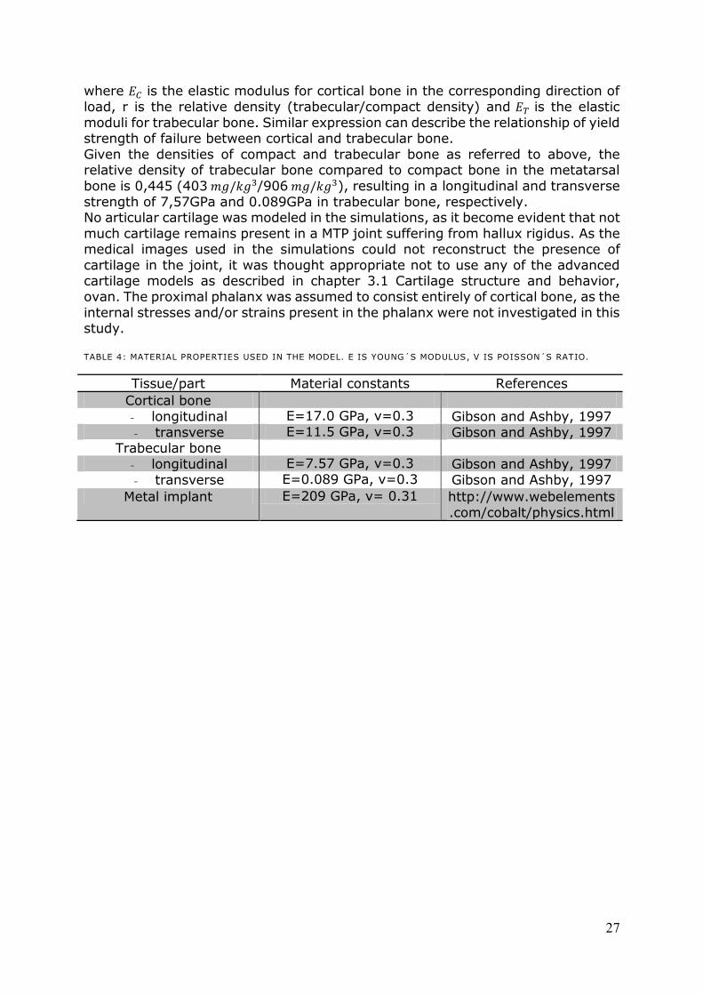
27

where is the elastic modulus for cortical bone in the corresponding direction of

load, r is the relative density (trabecular/compact density) and is the elastic

moduli for trabecular bone. Similar expression can describe the relationship of yield strength of failure between cortical and trabecular bone.

Given the densities of compact and trabecular bone as referred to above, the relative density of trabecular bone compared to compact bone in the metatarsal

bone is 0,445 (403 /906 ), resulting in a longitudinal and transverse

strength of 7,57GPa and 0.089GPa in trabecular bone, respectively. No articular cartilage was modeled in the simulations, as it become evident that not

much cartilage remains present in a MTP joint suffering from hallux rigidus. As the medical images used in the simulations could not reconstruct the presence of

cartilage in the joint, it was thought appropriate not to use any of the advanced cartilage models as described in chapter 3.1 Cartilage structure and behavior, ovan. The proximal phalanx was assumed to consist entirely of cortical bone, as the

internal stresses and/or strains present in the phalanx were not investigated in this study.

TABLE 4: MATERIAL PROPERTIES USED IN THE MODEL. E IS YOUNG´S MODULUS, V IS POISSON´S RATIO.

Tissue/part Material constants References

Cortical bone

- longitudinal E 17.0 Pa, v 0. Gibson and Ashby, 1997

- transverse E 11. Pa, v 0. Gibson and Ashby, 1997 Trabecular bone

- longitudinal E 7. 7 Pa, v 0. Gibson and Ashby, 1997

- transverse E 0.08 Pa, v 0. Gibson and Ashby, 1997

Metal implant E 0 Pa, v 0. 1 http://www.webelements

.com/cobalt/physics.html

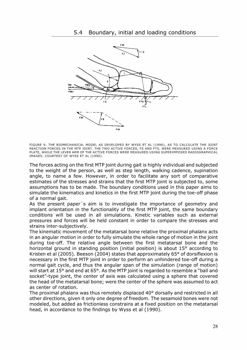
28

5.4 Boundary, initial and loading conditions

FIGURE 9: THE BIOMECHANICAL MODEL AS DEVELOPED BY WYSS ET AL (1990), AS TO CALCULATE THE JOINT

REACTION FORCES IN THE MTP JOINT. THE TWO ACTIVE FORCES, FS AND FTS, WERE MEASURED USING A FORCE

PLATE, WHILE THE LEVER ARM OF THE ACTIVE FORCES WERE MEASURED USING SUPERIMPOSED RADIOGRAPHICAL

IMAGES. COURTESY OF WYSS ET AL (1990).

The forces acting on the first MTP joint during gait is highly individual and subjected

to the weight of the person, as well as step length, walking cadence, supination angle, to name a few. However, in order to facilitate any sort of comparative

estimates of the stresses and strains that the first MTP joint is subjected to, some assumptions has to be made. The boundary conditions used in this paper aims to simulate the kinematics and kinetics in the first MTP joint during the toe-off phase

of a normal gait. As the present paper´s aim is to investigate the importance of geometry and

implant orientation in the functionality of the first MTP joint, the same boundary conditions will be used in all simulations. Kinetic variables such as external pressures and forces will be held constant in order to compare the stresses and

strains inter-subjectively. The kinematic movement of the metatarsal bone relative the proximal phalanx acts

in an angular motion in order to fully simulate the whole range of motion in the joint during toe-off. The relative angle between the first metatarsal bone and the horizontal ground in standing position (initial position) is about 15° according to

Kristen et al (2005). Beeson (2004) states that approximately 65° of dorsiflexion is necessary in the first MTP joint in order to perform an unhindered toe-off during a

normal gait cycle, and thus the angular span of the simulation (range of motion) will start at 1 ° and end at 6 °. As the MTP joint is regarded to resemble a “ball and socket”-type joint, the center of axis was calculated using a sphere that covered

the head of the metatarsal bone; were the center of the sphere was assumed to act as center of rotation.

The proximal phalanx was thus remotely displaced 40° dorsally and restricted in all other directions, given it only one degree of freedom. The sesamoid bones were not

modeled, but added as frictionless constrains at a fixed position on the metatarsal head, in accordance to the findings by Wyss et al (1990).

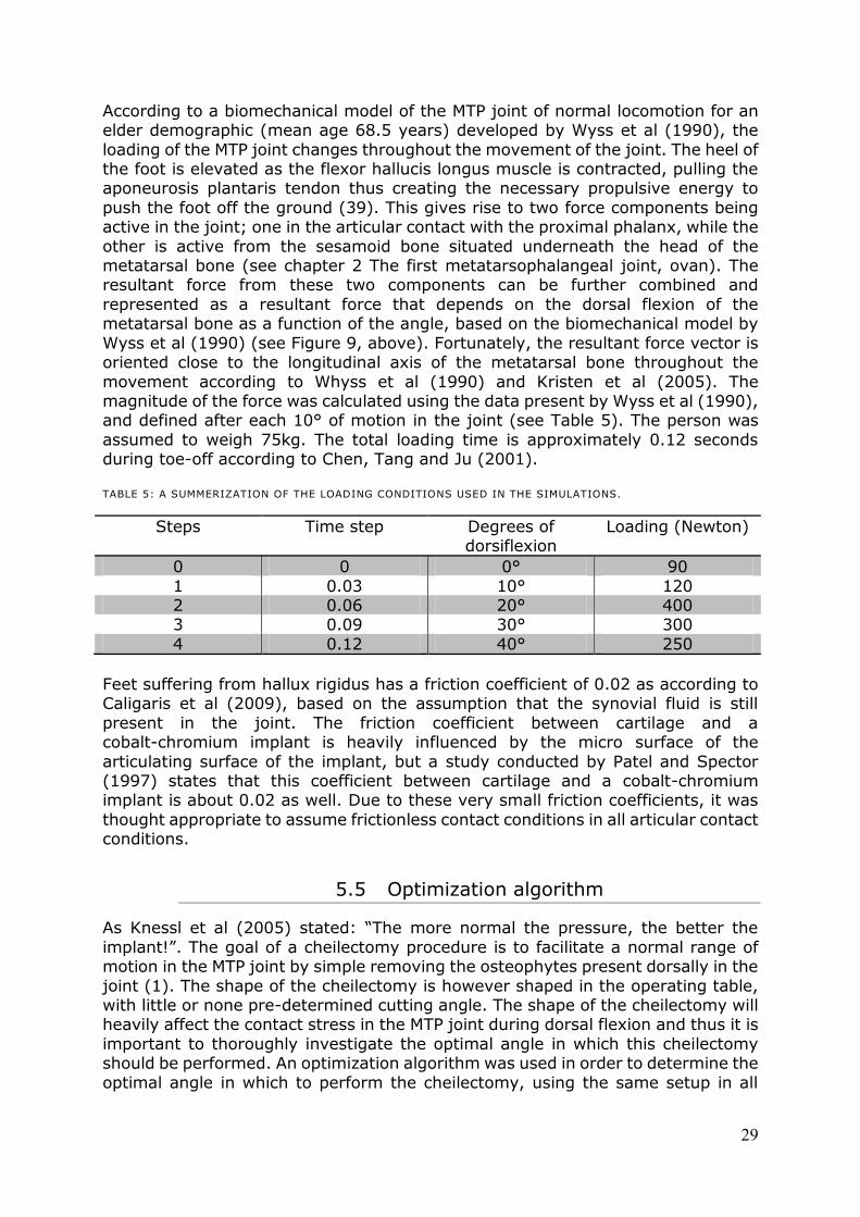
29

According to a biomechanical model of the MTP joint of normal locomotion for an elder demographic (mean age 68.5 years) developed by Wyss et al (1990), the

loading of the MTP joint changes throughout the movement of the joint. The heel of the foot is elevated as the flexor hallucis longus muscle is contracted, pulling the aponeurosis plantaris tendon thus creating the necessary propulsive energy to

push the foot off the ground (39). This gives rise to two force components being active in the joint; one in the articular contact with the proximal phalanx, while the

other is active from the sesamoid bone situated underneath the head of the metatarsal bone (see chapter 2 The first metatarsophalangeal joint, ovan). The resultant force from these two components can be further combined and

represented as a resultant force that depends on the dorsal flexion of the metatarsal bone as a function of the angle, based on the biomechanical model by

Wyss et al (1990) (see Figure 9, above). Fortunately, the resultant force vector is oriented close to the longitudinal axis of the metatarsal bone throughout the

movement according to Whyss et al (1990) and Kristen et al (2005). The magnitude of the force was calculated using the data present by Wyss et al (1990), and defined after each 10° of motion in the joint (see Table 5). The person was

assumed to weigh 75kg. The total loading time is approximately 0.12 seconds during toe-off according to Chen, Tang and Ju (2001).

TABLE 5: A SUMMERIZATION OF THE LOADING CONDITIONS USED IN THE SIMULATIONS.

Steps Time step Degrees of dorsiflexion

Loading (Newton)

0 0 0° 90

1 0.03 10° 120 2 0.06 20° 400 3 0.09 30° 300

4 0.12 40° 250

Feet suffering from hallux rigidus has a friction coefficient of 0.02 as according to Caligaris et al (2009), based on the assumption that the synovial fluid is still

present in the joint. The friction coefficient between cartilage and a cobalt-chromium implant is heavily influenced by the micro surface of the

articulating surface of the implant, but a study conducted by Patel and Spector (1997) states that this coefficient between cartilage and a cobalt-chromium implant is about 0.02 as well. Due to these very small friction coefficients, it was

thought appropriate to assume frictionless contact conditions in all articular contact conditions.

5.5 Optimization algorithm

As Knessl et al ( 00 ) stated: “The more normal the pressure, the better the

implant!”. The goal of a cheilectomy procedure is to facilitate a normal range of motion in the MTP joint by simple removing the osteophytes present dorsally in the

joint (1). The shape of the cheilectomy is however shaped in the operating table, with little or none pre-determined cutting angle. The shape of the cheilectomy will heavily affect the contact stress in the MTP joint during dorsal flexion and thus it is

important to thoroughly investigate the optimal angle in which this cheilectomy should be performed. An optimization algorithm was used in order to determine the

optimal angle in which to perform the cheilectomy, using the same setup in all

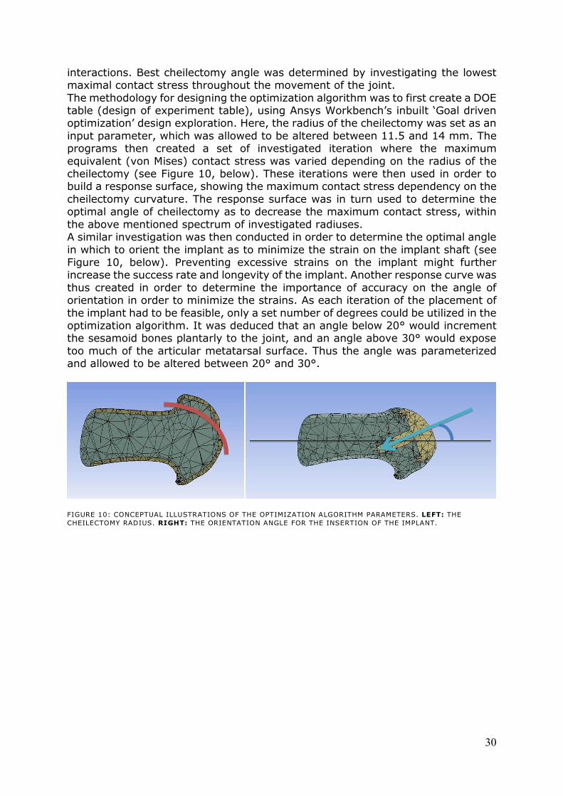
30

interactions. Best cheilectomy angle was determined by investigating the lowest maximal contact stress throughout the movement of the joint.

The methodology for designing the optimization algorithm was to first create a DOE table (design of experiment table), using Ansys Workbench’s inbuilt ‘ oal driven optimization’ design exploration. Here, the radius of the cheilectomy was set as an

input parameter, which was allowed to be altered between 11.5 and 14 mm. The programs then created a set of investigated iteration where the maximum

equivalent (von Mises) contact stress was varied depending on the radius of the cheilectomy (see Figure 10, below). These iterations were then used in order to build a response surface, showing the maximum contact stress dependency on the

cheilectomy curvature. The response surface was in turn used to determine the optimal angle of cheilectomy as to decrease the maximum contact stress, within

the above mentioned spectrum of investigated radiuses. A similar investigation was then conducted in order to determine the optimal angle

in which to orient the implant as to minimize the strain on the implant shaft (see Figure 10, below). Preventing excessive strains on the implant might further increase the success rate and longevity of the implant. Another response curve was

thus created in order to determine the importance of accuracy on the angle of orientation in order to minimize the strains. As each iteration of the placement of

the implant had to be feasible, only a set number of degrees could be utilized in the optimization algorithm. It was deduced that an angle below 20° would increment the sesamoid bones plantarly to the joint, and an angle above 30° would expose

too much of the articular metatarsal surface. Thus the angle was parameterized and allowed to be altered between 20° and 30°.

FIGURE 10: CONCEPTUAL ILLUSTRATIONS OF THE OPTIMIZATION ALGORITHM PARAMETERS. LEFT: THE

CHEILECTOMY RADIUS. RIGHT: THE ORIENTATION ANGLE FOR THE INSERTION OF THE IMPLANT.

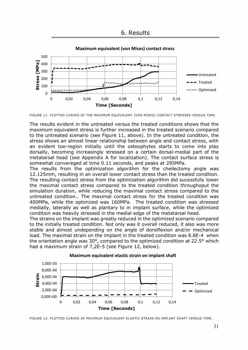
31

6. Results

FIGURE 11: PLOTTED CURVES OF THE MAXIMUM EQUIVALENT (VON MISES) CONTACT STRESSES VERSUS TIME.

The results evident in the untreated versus the treated conditions shows that the

maximum equivalent stress is further increased in the treated scenario compared to the untreated scenario (see Figure 11, above). In the untreated condition, the stress shows an almost linear relationship between angle and contact stress, with

an evident toe-region initially until the osteophytes starts to come into play dorsally, becoming increasingly stressed on a certain dorsal-medial part of the

metatarsal head (see Appendix A for localization). The contact surface stress is somewhat convereged at time 0.11 seconds, and peaks at 295MPa. The results from the optimization algorithm for the cheilectomy angle was

12.125mm, resulting in an overall lower contact stress than the treated condition. The resulting contact stress from the optimization algorithm did sucessfully lower

the maximal contact stress compared to the treated condition throughoput the simulation duration, while reducing the maximal contact stress compared to the untreated condition.. The maximal contact stress for the treated condition was

400MPa, while the optimized was 160MPa. The treated condition was stressed medially, laterally as well as plantary to in implant surface, while the optimized

condition was heavily stressed in the medial edge of the metatarsal head. The strains on the implant was greatly reduced in the optimized scenario compared to the initially treated condition. Not only was it overall reduced, it also was more

stable and almost undepending on the angle of dorsiflexion and/or mechanical load. The maximal strain on the implant in the treated condition was 8.8E-4 when

the orientation angle was 30°, compared to the optimized condition at 22.5° which had a maximum strain of 7,2E-5 (see Figure 12, below).

FIGURE 12: PLOTTED CURVES OF MAXIMUM EQUIVALENT ELASTIC STRAIN ON IMPLANT SHAFT VERSUS TIME.

0

100

200

300

400

500

0 0,02 0,04 0,06 0,08 0,1 0,12 0,14

Str

ess [

MP

a]

Time [Seconds]

Maximum equivalent (von Mises) contact stress

Untreated

Treated

Optimized

0,00E+00

2,00E-04

4,00E-04

6,00E-04

8,00E-04

1,00E-03

0 0,02 0,04 0,06 0,08 0,1 0,12 0,14

Str

ain

Time [Seconds]

Maximum equivalent elastic strain on implant shaft

Treated

Optimized

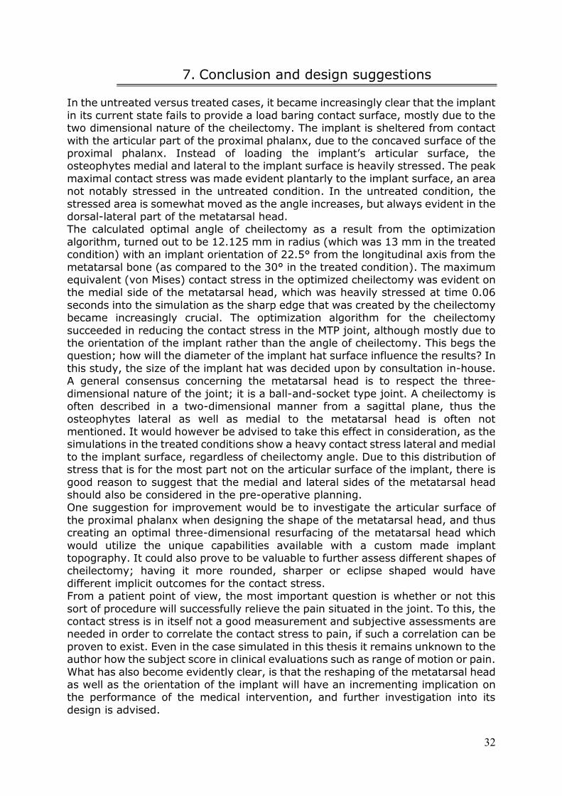
32

7. Conclusion and design suggestions

In the untreated versus treated cases, it became increasingly clear that the implant

in its current state fails to provide a load baring contact surface, mostly due to the two dimensional nature of the cheilectomy. The implant is sheltered from contact

with the articular part of the proximal phalanx, due to the concaved surface of the proximal phalanx. Instead of loading the implant’s articular surface, the osteophytes medial and lateral to the implant surface is heavily stressed. The peak

maximal contact stress was made evident plantarly to the implant surface, an area not notably stressed in the untreated condition. In the untreated condition, the

stressed area is somewhat moved as the angle increases, but always evident in the dorsal-lateral part of the metatarsal head. The calculated optimal angle of cheilectomy as a result from the optimization

algorithm, turned out to be 12.125 mm in radius (which was 13 mm in the treated condition) with an implant orientation of 22.5° from the longitudinal axis from the

metatarsal bone (as compared to the 30° in the treated condition). The maximum equivalent (von Mises) contact stress in the optimized cheilectomy was evident on the medial side of the metatarsal head, which was heavily stressed at time 0.06

seconds into the simulation as the sharp edge that was created by the cheilectomy became increasingly crucial. The optimization algorithm for the cheilectomy

succeeded in reducing the contact stress in the MTP joint, although mostly due to the orientation of the implant rather than the angle of cheilectomy. This begs the question; how will the diameter of the implant hat surface influence the results? In

this study, the size of the implant hat was decided upon by consultation in-house. A general consensus concerning the metatarsal head is to respect the three-

dimensional nature of the joint; it is a ball-and-socket type joint. A cheilectomy is often described in a two-dimensional manner from a sagittal plane, thus the

osteophytes lateral as well as medial to the metatarsal head is often not mentioned. It would however be advised to take this effect in consideration, as the simulations in the treated conditions show a heavy contact stress lateral and medial

to the implant surface, regardless of cheilectomy angle. Due to this distribution of stress that is for the most part not on the articular surface of the implant, there is

good reason to suggest that the medial and lateral sides of the metatarsal head should also be considered in the pre-operative planning. One suggestion for improvement would be to investigate the articular surface of

the proximal phalanx when designing the shape of the metatarsal head, and thus creating an optimal three-dimensional resurfacing of the metatarsal head which

would utilize the unique capabilities available with a custom made implant topography. It could also prove to be valuable to further assess different shapes of cheilectomy; having it more rounded, sharper or eclipse shaped would have

different implicit outcomes for the contact stress. From a patient point of view, the most important question is whether or not this

sort of procedure will successfully relieve the pain situated in the joint. To this, the contact stress is in itself not a good measurement and subjective assessments are needed in order to correlate the contact stress to pain, if such a correlation can be

proven to exist. Even in the case simulated in this thesis it remains unknown to the author how the subject score in clinical evaluations such as range of motion or pain.

What has also become evidently clear, is that the reshaping of the metatarsal head as well as the orientation of the implant will have an incrementing implication on the performance of the medical intervention, and further investigation into its

design is advised.

33

8. Analysis and validation

As in all FE analyses, the outcome is only approximate rather than an exact

solution. Some approximations and simplifications will always be evident, no less so in biomechanical applications. Apparent limitations in the present study should

be made clear to the reader; no soft tissues such as ligaments, tendons or muscles were modeled; the sesamoid bones were not represented; the hallux (big toe) was assumed to move in a linear velocity throughout the movement as well as being

limited to one degree of freedom; the implant was assumed to be totally fixated and fully osseointegrated into the trabecular bone; the force components were

simplified and represented as a resultant vector force; viscoelastic effects were neglected, as well as other environmental factors. Such limitations and apparent simplifications in numerical methods are of outmost necessity, but most always be

weighed against the problem and question being investigated. For example, no cartilage models were used in the conceived simulations, as clinical

implementations has concluded that cartilage is in most hallux rigidus cases, all but totally worn out. The medical images failed to determine if this particular case had any cartilage left, and as so the simulations was conducted without any cartilage

model as described in chapter 3.1 Cartilage structure and behavior, ovan. Some of these approximations and simplifications would need to be further investigated

upon in order to produce more reliable results, but thought to be justifiable in this novel configuration. Another factor to consider is the data used in the formulation of the boundary

conditions, as using data from different data sets should always be viewed with skepticism. Seldom does the data fully coincide, as they are all based on different

estimations and from different investigating aspects. For example, the density of the metatarsal bone used in this study derived from Gutekunst et al

(UNPUBLISHED), who studied the bone density of the second metatarsal bone, and not the first as the one modeled. Similarly, the results evident in the article by Whyss et al (1990) were based on an elder population, which might not be the ideal

demographic group to base the boundary conditions on as they might have restraining joint defects (although they were deemed as healthy without foot

impairments in the article). Whyss et al (1990) do comment on this factor as they compare their results with another similar study that was conducted on a significantly younger age group. The two studies does show deviating results, as

Whyss’s research expressed significantly lower joint reaction forces (about 0% of weight) compared to the younger demographic group (about 80% of weight) (39).

Given the patient demographic in question, it was though appropriate to base the boundary conditions on the older demographic population rather than that of the younger. Without proper insight into each and every referred article, is it borderline

impossible to determine how the different setups used in their respective research were denoted.

Validating the model and the results were indeed tricky, as no apparent similar study could be found by the author. There exist a number of high-order finite element models of feet, but none investigating the same phenomenon as present in

this thesis. Chen (2011) submitted in his master thesis a very detailed foot model to be used to analyze the occurrence of stress fractures on the metatarsal bones,

by using medical reconstructed images to model the bones and spring elements to simulate tendons and ligaments. However, Chen used a static structural setup, which does not capture movement in the joint, nor does his research encapsulate

34

the joint contact stress as he investigates the effect of the length of the metatarsal bone on the risk of developing stress fractures.

A perhaps more relevant study was conducted by Kristen et al (2005), which aimed to study the loading of the first metatarsal bone during toe-off by designing a FE model of a cadaveric foot from a 44-year-old female, who did not have any

deformity or signs of osteoarthritis in her MTP joint. The range of motion was not fully investigated, as Kristen et al (2005) instead analyzed three angles of

dorsiflexion in a static analysis, which further diminishes the influence of the geometrical shape of the metatarsal head. The study does however use very similar boundary conditions as present in this thesis. The results expressed in the article by

Kristen et al (2005) did somewhat coincide with the results evident in this thesis, as they also concurred that the maximum contact force in the MTP joint occurred at

maximum dorsiflexion (in their case at 70°), with an maximum load of 1000N. There were also some problems of technical nature, posing some unwanted

limitations in the expressed simulations. One such problem was to determine how the optimization algorithms were to be conducted as to automatically and autonomously be able to alternate the design of the cheilectomy and orientation of

the implant, and at all iterations recreate a functional model. This meant that refinements such as blends of edges could not be included, which might very well

have an incriminating effect in the simulations; the highest stresses present in the treated as well as optimized scenarios were evident in the sharp corners of the implant’s articular surface.

Due to all these limitations and validation issues, the modeled should not be viewed as able to fully represent an true MTP joint, but as an model to be used in

investigating the effect the metatarsal head geometry has in easing the contact stress in the MTP joint, and how the orientation of an implanted surface implant can be ideally placed in order to minimize the strains on the same implant. Even as it is

hard to suggest that the contact surface stresses evident in the results to be truly representative of the real scenario or to be used inter-subjectively, it is well enough

in order to determine the relative significance of the metatarsal head geometry in order to give suggestions in its geometrical shape, as well as to give suggestions on the implant angle orientation.

35

9. Discussion and future context

In the area of biomechanics, the use of the finite element method has become an

irreplaceable tool to be used in physiological analysis. Questions that could not be investigated before without invasive procedures (thus interfering with the

investigated area) or very approximate analytical calculations, can with the use of numerical methods be investigated with quite high fidelity. The current use of FEA is quite limited to understanding physiological phenomena; investigating fluid flows

and/or mechanical pressures (40; 41). In the field of dental applications however, the numerical method has increasingly been used to investigate and improve

implant design in order to further increase functionality (42; 43). It has also been increasingly popularized in implant assessments to determine stress shielding effects in various anatomical applications, mainly hip and knee but also such

peculiar placements i.e. ankles (44; 45). This move from pure research into product development has long been discussed in the biomechanical community,

where the use of patient specific simulations based on true medical image data can further improve treatment by designing patient specific drug disposal contraptions, surgery training modules and orthopedic custom made implants.

This paper serves as an example of a modern kind of biomechanical advancement; a case-driven application of engineered custom made orthopedic implant. To the

author´s knowledge, there is today no company currently on the market that design each and every implant based on case-specific medical images and simulations. Episurf Medical AB´s inspiring technology has the ability not only to

make every implant custom tailored for every patient and specific placement, but can with very high fidelity make sure that the implant is placed exactly at the right

position at the time of the operation. Implementing simulations into the process would however make it possible to even predict how well the expected result could

be after an operation, making it easier to determine what patient is likely to expect good results and thus suggest operation. The other part of this thesis was concerning the design of the implant, a common use of the finite element method

in other mechanical applications and only scratched upon in medical applications. Using simulations in product development has become a given methodology for the

engineer, as it saves time and money from the prototyping evaluations. It is also used in the development of orthopedic implant design, to a certain extent. The Episurf Medical AB´s implant has a custom made topography on its articular side

made after each individual patient, and thus running simulations in order to optimize this design would make an advanced tool to be used in the pre-planning

for the surgical intervention. The investigated parameters in this thesis were the equivalent (von Mises) stress evident on the contact surface of the joint, as well as the strain on the implant

shaft. Some correlation between stress and pain has been suggested in the literature, making it principally suggestible to try to lower this contact stress.

However, it is hard to determine how the subjected pain for the patient would be influenced simply by lowering the contact stress; it is unknown to the author how the patient that is simulated in this thesis score in clinical evaluations such as pain

or range of motion assessments. Investigating the strain on the implant shaft is commonly used in dental applications as to get an estimate on how the surrounding

tissue (bone) will get irritated, which could lower the functionality of the implant and its longevity. It is hard to determine if the strain put on the implant shaft could be regarded as hazardous, but efforts in reducing the strains could very well reduce

the chance for stress shielding and have an positive increment on the implant

36

longevity. A stress shielding effect can negatively affect the structure and density of the surrounding bone tissue, altering the metatarsal bone’s mechanical

properties negatively. The computational time for the simulations formulated in this thesis was 4 hours for the untreated condition and 5.5 hours for the treated condition, which would

become even longer if primed in more detail. However, the optimization algorithms took altogether days to compute, excluding the setup time needed to properly

execute and utilize the formulas. Some refinements of the simulations can and should be conducted, in order to produce more valuable data. One such improvement that would create significantly better and more trustworthy results

would be to determine the center of rotation by using moving x-ray images rather than trying to superimpose a sphere in position with the metatarsal head, as was

the case in this thesis. The sensitivity of the model would also have to be thoroughly investigated, as both a finer mesh and a lower time-step could very well

prove to be appropriate and produce more valid results. Further validations could also be conceived by simulating more hallux rigidus cases, as well as healthy MTP joints, in order to make more quantitative estimates

of the surgical intervention by comparing untreated, treated and healthy conditions. For this to be made conclusive, it would most likely be necessary to

include other clinical patient data as to correlate the results to the patient’s clinical findings and own assessment, especially that of pain. Making implant smaller and custom made demands high precision implementations

and smart manufacturing processes. As every human being is unique, the implant must also be custom tailored to each case. This sort of methodology is unheard of

on the market today, as it is not just simulation driven product development, but simulation driven case planning. The simulations can however be useful tools in order to assess and evaluate which patients are likely to benefit from such a

procedure as described in this paper, and who is to be advised to try other measures.

37

10. References

1. Hallux rigidus: aetiology, diagnosis, classification and treatment. Márquez, J

Asunción and Oliva, X Martin. 2010, Revista Española de Cirugía Ortopédica y

Traumatología 54, pp. 321-328.

2. Surgical Treatment of Hallux Rigidus Using a Metatarsal Head Resurfacing

Implant: Mid-term Follow-up. Carpenter, Brian, et al., et al. s.l. : The Journal of

Foot & Ankle Surgery, 2010, The Journal of Foot & Ankle Surgery 49, pp. 321-325.

310-325.

3. A Retrospective Analysis of Surgical Treatment in Patients With Symptomatic

Hallux Rigidus: Long-Term Follow-up. Beertema, Wieske, et al., et al. 2006, The

Journal of Foot & Ankle Surgery 45, pp. 244-251.

4. Hallux rigidus: A Cross-sectional study to evaluate clinical parameters. Beeson,

Paul, et al., et al. 2009, The Foot 19, pp. 80-92.

5. Resurfacing of the First Metatarsal Head in the Treatment of Hallux Rigidus.

Hasselman, Carl T and Shields, Naomi. 2008, Techniques in Foot & Ankle

Surgery 7, pp. 31-40.

6. Bojsen-Møller, Finn. Rörelseapparatens anatomi. s.l. : Liber AB, 2007.

7. Manda, Krishnagoud. Finite Element Simulations of Biphasic Articular

Cartilages with Localized Metal Implants. Stockholm : Universitetsservice US-AB,

2010.

8. Fluid Transport and Mechanical Properties of Articular Cartilage: A Review. Mow,

Van C, Holmest, Mark H and Lai, W Michael. 1984, Journal of Biomechanics 17,

pp. 377-394.

9. Anatomy and biomechanics of the foot and ankle. Dawe, Edward J C and

Davis, James. 2011, Orthopedics and Trauma 25, pp. 279-286.

10. The importance of the toes in walking. Hughes, Janet, Clark, Peter and

Klenerman, Leslie. 1990, Journal of Bone and Joint Surgery 2, pp. 245-251.

11. Pressure and force distribution characteristics under normal foot during the

push-off phase in gait. Hayafune, N, Hayafune, Y and Jacob, A C. 1999, The

Foot 9, pp. 88-92.

12. The surgical treatments of hallux limitus/rigidus: a critical review of the

literature. Beeson, P. 2004, The Foot 14, pp. 80-92.

13. The First Metatarsal Bone Loading Under Loading Conditions: A Finite Element

Analysis. Kristen, K H, et al., et al. 2005, Foot and Ankle Clinics 10, pp. 1-14.

14. Persson, Björn M and Wingstrand, Hans. Ortopedisk Grundbok. Sweden :

Studentlitteratur, 2005. pp. 35-37.

38

15. Relationship Between Articular Cartilage Damage and Bone Density in the First

Metatarsal. Bareither, Daniel, et al., et al. 1998, The Journal of Foot & Ankle

Surgery 37, pp. 401-409.

16. Classification systems for hallux rigidus: a review of the literature. Beeson,

Paul, et al., et al. 2008, Foot & Ankle International 29, pp. 407-414.

17. Clinical Rating Systems for the Ankle-Hindfoot, Midfoot, Hallux, and Lesser

Toes. Kitaoka, Harold B, et al., et al. 1994, Foot & Ankle International, pp.

349-353.

18. The Need for Surgical Revision After Isolated Cheilectomy for Hallux Rigidus: A

Systematic Review. Roukis, Thomas S. 2010, The Journal of Foot & Ankle Surgery

49, pp. 465-470.

19. Results of cheilectomy and additional microfracture technique for the treatment

of hallux rigidus. Becher, Christoph, Kilger, Robert and Thermann, Hajo.

2005, Foot and Ankle Surgery 11, pp. 155-160.

20. The Valenti Procedure for Hallux Limitus: A Long-Term Follow-up and Analysis.

Kurtz, Dorothy H, et al., et al. 1999, The Journal of Foot & Ankle Surgery 38, pp.

123-130.

21. First Metatarsophalangeal Arthrodesis for Treatment of Hallux Rigidus: A

Retrospective Study. Lombardi, Charles M, et al., et al. 2001, The Journal of

Foot & Ankle Surgery 40, pp. 137-143.

22. A novel pyrolytic carbon implant for hallux rigidus: A cadaveric study. Apard,

Thomas, et al., et al. 2011, Foot and Ankle Surgery 17, pp. 182-185.

23. BIOPRO Resurfacing Endoprosthesis Versus Periarticular Osteotomy for Hallux

Rigidus: Short-Term Follow-Up and Analysis. Roukis, Thomas S and Townley,

Charles O. 2003, The Journal of Foot & Ankle Surgery 42, pp. 350-358.

24. First Metatarsal Head Osteoarticular Transfer System for Salvage of a Failed

Hemicap-Implant: A Case Report. Hopson, Matthew, Stone, Paul and Paden,

Matthew. 2009, The Journal of Foot & Ankle Surgery 48, pp. 483-487.

25. Ground reaction forces under the great toe after implantation of the

TOEFIT-PLUS prosthesis. Knessl, Juerg, et al., et al. 2005, Foot and Ankle

Surgery 11, pp. 131-134.

26. Ratner, Buddy D, et al., et al. Biomaterials Science. London : Elsevier

Academic Press, 2004.

27. Integrative biomechanics: A paradigm for clinical applications of fundamental

mechanics. Ateshian, Gerard A and Friedman, Morton H. 2009, Journal of

Biomechanics 42, pp. 1444-1451.

28. Haut, Roger C. Biomechanics of Soft Tissues. [book auth.] Alan M Nahum and

John W Melvin. Accidental Injury: Biomechanics and Prevention. New York :

Springer Science + Business Media Inc, 2001, pp. 224-241.

39

29. Enderle, John, Blanchard, Susan and Bronzino, Joseph. Introduction to

Biomedical Engineering; Second Edition. Oxford : Elsevier Academic Press, 2005.

30. The generalized triphasic correspondence principle for simultaneous

determination of the mechanical properties and proteoglycan content of articular

cartilage by indentation. Lu, X Lux, et al., et al. 2007, Journal of Biomechanics

40, pp. 2434-2441.

31. Cartilage and diarthrodial joints as paradigms for hierarchical materials and

structures. Mow, Van C, Ratcliffe, Anthony and Poole, A Robin. 1992,

Biomaterials 13, pp. 67-97.

32. Elastic modulus and hardness of cortical and trabecular bovine bone measured

by nanoindentation. Wang, X J, et al., et al. 2006, Transactions of Nonferrous

Metals Society of China 16, pp. 744-748.

33. Mechanical properties and the hierichial structure of bone. Rho, Jay-Toung,

Kuhn-Spearing, Liisa and Zioupos, Peter. 1998, Medical Engineering & Physics

20, pp. 92-102.

34. Currey, John D. The Mechanical Adaptations of Bones. s.l. : Princeton

University Press, 1984.

35. Elastic modulus and hardness of cortical and trabecular bone lamellae

measured by nanoindentation in the human femur. Zysset, Philippe K, et al., et

al. 1999, Journal of Biomechanics 32, pp. 1005-1012.

36. Gibson, Lorna J and Ashby, Michael F. Cellular solids: Structure and

properties - Second edition. Cambridge : Cambridge University Press, 1997.

37. Role of mechanical environment and implant design on bone tissue

differentiation: current knowledge and future contexts. Cehreli, Murat, Sahin,

Saime and Akca, Kivanc. 2004, Journal of Dentistry 32, pp. 123-132.

38. Surface treatments of titanium dental implants for rapid osseointegration.

Guéhennec, L Le, et al., et al. 2007, Dental materials 23, pp. 844-854.

39. Joint reaction forces at the first mtp joint in a normal elderly population. Wyss,

U P, et al., et al. 1990, Journal of Biomechanics 23, pp. 997-984.

40. Finite element analysis of human and artificial articular cartilage. Abbass,

Sadiq Jafer and Abdulateef, Farah Mohammed Reda. 2012, Journal of

Engineering 4, pp. 443-458.

41. Finite Element simulations of a focal knee resurfacing implant applied to

localized cartilage defects in a sheep model. Manda, Krishnagoud, Ryd, Leif and

Eriksson, Anders. 2011, Journal of Biomechanics 44, pp. 794-801.

42. Bone stress and interfacial sliding analysis of implant designs on an

immediately loaded maxillary implant: A non-linear finite element study. Huang,

Heng-Li, et al., et al. 2008, Journal of Dentistry 36, pp. 409-417.

40

43. The influence of functional forces on the biomechanics of implant-supported

prostheses - a review. Sahin, Saime, Cehreli, Murat C and Yalcin, Emine.

2002, Journal of Dentistry 30, pp. 271-282.

44. Finite element stress analysis of some ankle joint prostheses. Falsig, Jette,

Hvid, Ivan and Jensen, Niels Chr. 1986, Clinical Biomechanics 1, pp. 71-76.

45. Numerical simulation of strain-adaptive bone remodelling in the ankle joint.

Bouguecha, Anas, et al., et al. 2011, BioMedical Engineering OnLine 10, pp.

1-13.

46. Contributions of Bone Density and Geometry to the Strenght of the Human

Second Metatarsal. Muehleman, C, et al., et al. 2000, Bone 27, pp. 709-714.

47. Predicting ex vivo failure loads in human metatarsals using bone strength

indices derived from volumetric quantitative computer tomography. Gutekunst,

David J, et al., et al. Unpublished, 2012, Journal of Biomechanics.

48. Investigation of the Frictional Response of Osteoarthritic Human Tibiofemoral

Joints and the Potential Beneficial Tribological Effect of Healthy Synovial Fluid.

Caligaris, Matteo, et al., et al. 2009, Osteoarthritis Cartilage 17, pp. 1327-1332.

49. Tribological evaluation of oxidized zirconium using an articular cartilage

counterface: a novel material for potential use in hemiarthroplasty. Patel, A M

and Spector, M. 1997, Biomaterials 18, pp. 441-447.

50. Finite Element Analysis of the Foot: Metatarsal geometry and indication for

stress fractures. Chen, Raymond Guanway. 2011, Unpublished master's thesis,

University of Medicine and Dentistry of New Jersey and Rutgers the State

University of New Jersey, New Jersey, USA.

51. Stress distribution of the foot during mid-stance to push-off in barefoot gait: a

3-D finite element analysis. Chen, Weng-Pin, Tang, Fuk-Tan and Ju,

Chia-Wei. 2001, Clinical Biomechanics 16, pp. 614-620.

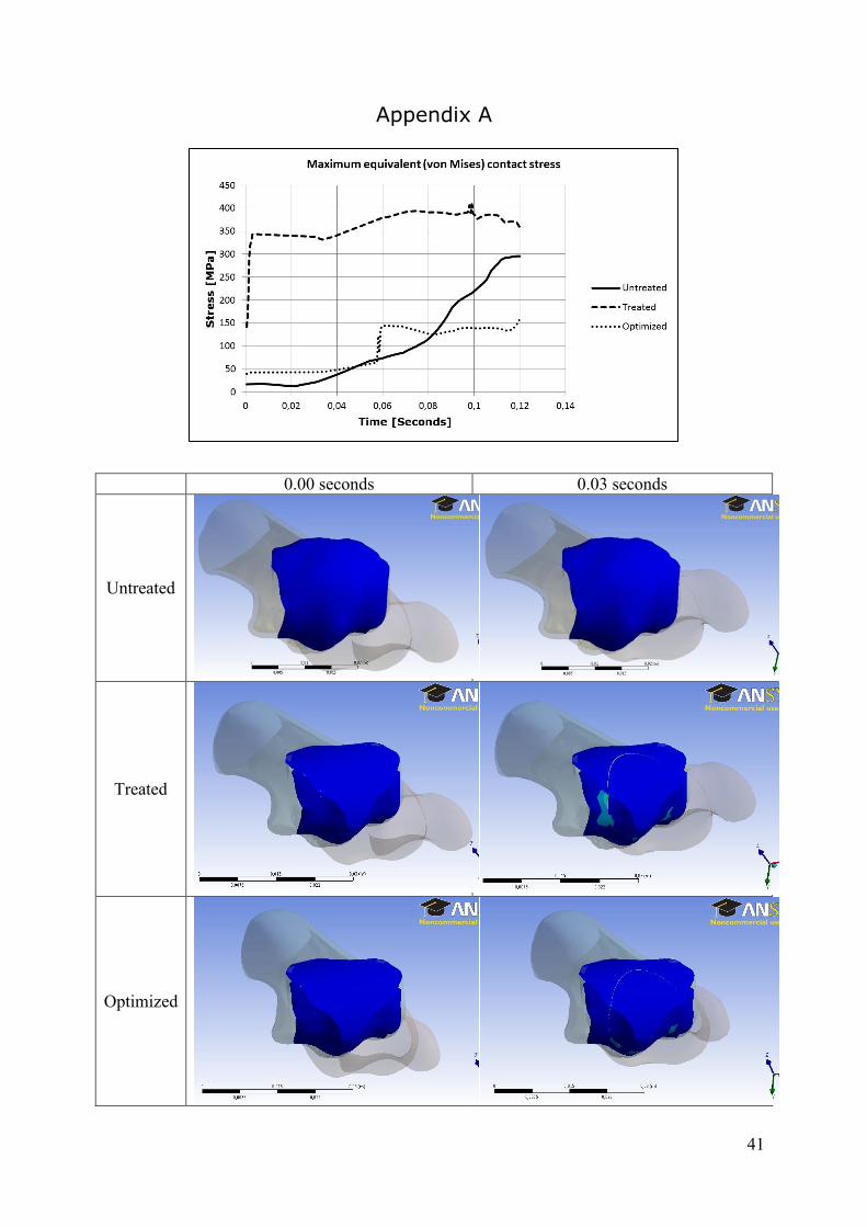
41

Appendix A

0.00 seconds 0.03 seconds

Untreated

Treated

Optimized

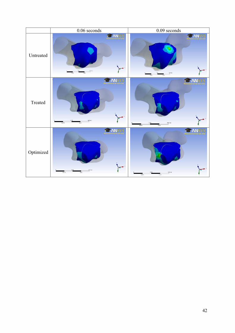
42

0.06 seconds 0.09 seconds

Untreated

Treated

Optimized

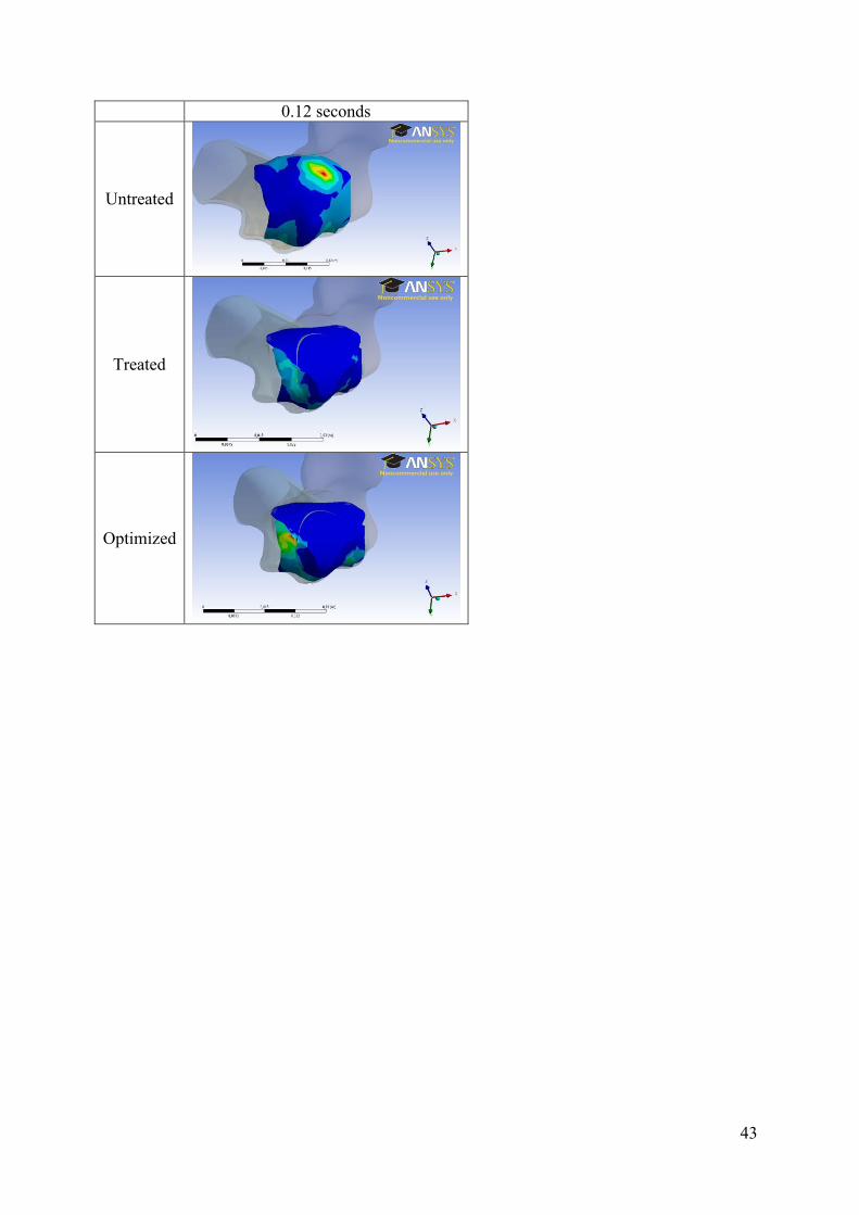
43

0.12 seconds

Untreated

Treated

Optimized