Embed Size (px)
Citation preview

Lorenzo Bretscher, Christian Julliard and Carlo Rosa
Human capital and international portfolio diversification: a reappraisal Article (Published version) (Refereed)
Original citation: Bretscher, Lorenzo, Julliard, Christian and Rosa, Carlo (2016) Human capital and international portfolio diversification: a reappraisal. Journal of International Economics, 99 (1). S78-S96. ISSN 0022-1996 DOI: 10.1016/j.jinteco.2015.12.007 Reuse of this item is permitted through licensing under the Creative Commons:
© 2016 Elsevier CC-BY This version available at: http://eprints.lse.ac.uk/64835/ Available in LSE Research Online: February 2016
LSE has developed LSE Research Online so that users may access research output of the School. Copyright © and Moral Rights for the papers on this site are retained by the individual authors and/or other copyright owners. You may freely distribute the URL (http://eprints.lse.ac.uk) of the LSE Research Online website.

Journal of International Economics xxx (2015) xxx–xxx
ARTICLE IN PRESSINEC-02919; No of Pages 19
Contents lists available at ScienceDirect
Journal of International Economics
j ourna l homepage: www.e lsev ie r .com/ locate / j i e
Human capital and international portfolio diversification: A reappraisal✩
Lorenzo Bretschera, Christian Julliarda,∗,1, Carlo Rosab
aDepartment of Finance, SRC and FMG, London School of Economics, Houghton Street, London WC2A 2AE, United KingdombMarkets Group, Federal Reserve Bank of New York, 33 Liberty Street, New York, NY 10045, United States
A R T I C L E I N F O
Article history:Received 21 August 2015Received in revised form 10 December 2015Accepted 22 December 2015Available online xxxx
JEL Classification:E21F30G11G15
Keywords:Home country biasIncomplete marketsInternational diversification puzzleNon-traded human capitalHedging human capitalOptimal portfolio choice
A B S T R A C T
We study the implications of human capital hedging for international portfolio choice. First, we documentthat, at the household level, the degree of home country bias in equity holdings is increasing in the laborincome to financial wealth ratio. Second, we show that a heterogeneous agent model in which householdsface short selling constraints and labor income risk, calibrated to match both micro and macro labor incomeand asset returns data, can both rationalize this finding and generate a large aggregate home country biasin portfolio holdings. Third, we find that the empirical evidence supporting the belief that the human cap-ital hedging motive should skew domestic portfolios toward foreign assets, is driven by an econometricmisspecification rejected by the data.
© 2015 The Authors. Published by Elsevier B.V. This is an open access article under the CC BY license(http://creativecommons.org/licenses/by/4.0/).
“Human wealth is likely to be about two-thirds of total wealthand twice financial wealth. This suggests that the omission ofhuman wealth may be a serious matter.”
[Campbell (1996)]
✩ This paper is based upon, and replaces, two companion papers: “The InternationalDiversification Puzzle is not Worse Than You Think” and “Human Capital and Inter-national Portfolio Choice.” We thank Laura Bottazzi, Charles Engel, Jeffrey Frankel,Filiz Garip, Francesco Giavazzi, Sebnem Kalemli-Özcan, Per Krusell, Alex Michaelides,Jonathan Parker, Aureo de Paula, Udara Peiris, Marcelo Pinheiro, Hélène Rey, Christo-pher Sims, Kenneth West, Noah Williams and seminar participants at the LondonSchool of Economics, Princeton University, Tokyo University, 2015 NBER InternationalSeminar on Macroeconomics, and the LFE ICEF Finance Conference, for helpful discus-sions and comments. The views expressed in this paper are those of the authors anddo not necessarily reflect the position of the Federal Reserve Bank of New York or theFederal Reserve System.
* Corresponding author.E-mail addresses: [email protected] (L. Bretscher), [email protected]
(C. Julliard), [email protected] (C. Rosa).URLs: http://personal.lse.ac.uk/julliard (C. Julliard),
http://nyfedeconomists.org/rosa (C. Rosa).1 Christian Julliard thanks the Economic and Social Research Council (UK) [grant
number: ES/K002309/1] for financial support.
1. Introduction
International finance theory emphasizes the effectiveness ofglobal portfolio diversification strategies for cash-flow stabilizationand consumption risk sharing.2 However, the empirical evidence oninternational portfolio holdings favors a widespread lack of diversi-fication across countries and a systematic bias toward home countryassets (see, e.g., Coeurdacier and Rey, 2013 for a recent survey). Thisdiscrepancy between theoretical predictions and observed portfolioconstitutes the international diversification puzzle (see, e.g., Frenchand Poterba, 1991).
2 Nevertheless, the size of gains from international risk sharing continues to be adebated issue. E.g.: Grauer and Hakansson (1987) suggest that an individual’s gainsfrom international stock-portfolio diversification are large; Cole and Obstfeld (1991)find small gains from perfect pooling of output risks; Obsfteld (1994) calibration exer-cises imply that most countries reap large steady-state welfare gains from globalfinancial integration; Palacios-Huerta (2001) finds that, for a mean variance investor,adding human capital to the definition of wealth generates substantially smaller gainsfrom international portfolio diversification.
http://dx.doi.org/10.1016/j.jinteco.2015.12.0070022-1996/© 2015 The Authors. Published by Elsevier B.V. This is an open access article under the CC BY license (http://creativecommons.org/licenses/by/4.0/).
Please cite this article as: L. Bretscher, et al., Human capital and international portfolio diversification: A reappraisal, Journal of InternationalEconomics (2015), http://dx.doi.org/10.1016/j.jinteco.2015.12.007

2 L. Bretscher, et al. / Journal of International Economics xxx (2015) xxx–xxx
ARTICLE IN PRESS
Moreover, albeit the degree of home bias has been reducing dur-ing the last few decades, it remains a first order characteristic ofportfolio holdings.3
In the major industrialized countries, roughly two-thirds of grossdomestic product goes to labor and only one-third to capital. Thus,human wealth likely constitutes about two-thirds of total wealth,suggesting that if investors attempt to hedge against adverse fluctua-tions in returns to human capital when making financial investmentdecisions, the mere size of human capital in total wealth makes itspotential impact on portfolio holdings self-evident.
Based on this observation, several contributions have argued thatwhen the role of human capital is explicitly taken into account, theobserved home country bias in portfolio holdings becomes harderto rationalize. The argument, originally formalized by Brainard andTobin (1992) with a stylized example, works as follows: if returns tohuman capital are more correlated with the domestic stock marketthan with the foreign ones, labor income risk can be more effectivelyhedged with foreign assets than with domestic ones, and equilib-rium portfolio holdings should be skewed toward foreign securities.4
As emphasized by Cole (1988), “this result is disturbing, given theapparent lack of international diversification that we observe.”
However, as first suggested in Bottazzi et al. (1996), human cap-ital hedging could also lead toward home country bias in portfolioholdings. For instance, the correlation between domestic return onphysical and human capital can be lowered by idiosyncratic shocksthat lead to a redistribution of total income between capital andlabor. In the presence of these rent shifting shocks, foreign assetsbecome a less attractive hedge for labor income risk—especially iftotal factor productivity shocks are highly correlated internationally.If the size of the rent shifting shocks is large enough, a situation inwhich domestic assets are the best hedge against human capital riskarises, therefore leading to home country bias in portfolio holdings.
In this paper, we ask whether the human capital hedging motiveis likely to have a sizeable effect on optimal portfolio choice, andwhat its implications are for the international diversification puzzle.Moreover, we propose a rationalization of the home country bias,based on a setting of endogenous portfolio formation and incompletemarkets, that not only can rationalize aggregate portfolio holdings,but also the variable degree of home country bias in households’portfolios.
In particular, Fig. 1 depicts a novel (to the best of our knowl-edge) finding about households’ equity home bias.5 Panel (a) depictsthe (locally weighted regression of the) share of foreign assets inU.S. household portfolios as a function of the household financialwealth to labor income ratio. Since (labor income) flows and stocks(of human capital) are cointegrated, Panel (a) shows that there is asystematic relationship between household specific home countrybias and the household specific financial to human capital ratio: thedegree of home country bias monotonically decreases as the humancapital component of household total wealth becomes smaller rela-tive to the household financial wealth. That is, in micro data, whenthe human capital hedging motive is more prominent relative tothe financial wealth hedging motive, household portfolios show ahigher degree of home country bias. Moreover, panel (b) of Fig. 1, thatdepicts the (locally weighted regression of the) number of stocks
3 Coeurdacier and Rey (2013, Table 1) estimate that, for a large set of countries,the 2008 portfolio share in domestic equity is on average about 71%, with an aver-age implied home bias (measured as one minus the ratio of domestic equities in thedomestic portfolio relative to the the domestic share in world market capitalization)of about 70%.
4 Moreover, Michaelides (2003) shows with a calibration exercise that, in the pres-ence of liquidity constraints, if labor income shocks are positively correlated withthe domestic stock market returns and orthogonal to foreign asset returns, investorsshould hold only foreign assets in their portfolios.
5 We are thankful to Laura Bottazzi and Sebnem Kalemli-Özcan for suggesting us toexplore this dimension of the data.
in U.S. household portfolios as a function of the household finan-cial wealth to labor income ratio, shows that when the households’human capital wealth is relative larger than the financial wealth, thehousehold portfolio will tend to be overall less diversified.
Our paper provides a rationalization of both of these findings,as well as of the aggregate home country bias, and also shows thatthe canonical intuition that human capital should skew portfolioholdings toward foreign assets, and the related supporting empiri-cal evidence, are both very fragile. In particular, we offer two maincontributions.
First, using novel estimates of the correlations of human capi-tal and stock market return innovations, we calibrate an incompletemarket model in which agents face both idiosyncratic and aggregatelabor income risk, as well as borrowing constraints.6 The model isalso calibrated to match the microeconomic (following Gourinchasand Parker, 2002) characteristics of the U.S. labor income and trackthe distribution of the asset wealth to labor income ratios observedin the Panel Study of Income Dynamics (PSID).
The main findings of this calibration exercise are that a) investorsthat enter the stock market with a low level of liquid (i.e. finan-cial) wealth to labor income ratio will initially specialize in domesticassets and, b) only as the level of asset wealth to labor income ratioincreases do agents start diversifying their portfolios internation-ally by progressively adding different assets to their holdings, c) as aconsequence, the aggregate portfolio of U.S. investors shows a largedegree of home bias.
What drives these results? Households face large human capitalrisk, but this is mostly of the idiosyncratic type—hence underesti-mated in a homogeneous agent setting. Moreover, in the presence ofliquidity constraints, agents cannot borrow to construct an optimallydiversified portfolio. Therefore, when their level of liquid wealthto labor income ratio is sufficiently high and they enter the stockmarket, agents try to minimize the overall wealth risk, investingfirst in the asset that has the lowest degree of correlation with laborincome innovations—and, as discussed below, this assets is, in thedata, the domestic stock. Only when the ratio of liquid wealth tolabor income is sufficiently high, and the labor income risk hedgingmotive becomes less important relative to the financial risk hedgingone, do agents start investing in foreign assets and diversifying theirportfolios internationally. Since the distribution of liquid wealth tolabor income is (in the data as in the model) concentrated in theregion of low liquid wealth to labor income ratios, the resultingaggregate portfolio is heavily skewed toward domestic assets. Notethat, in the absence of market frictions and idiosyncratic risk, theestimated and calibrated correlations of labor income and returnsinnovations, being very small, would have almost no effect on theoptimal portfolios.
Moreover, since in our model the aggregate home country biasdepends on both the household optimal investment policy functionsand the aggregate distribution of liquid wealth to labor income, atrend of increasing concentration of financial wealth (as documentedby Piketty, 2014), and/or a negative trend in the labor share ofincome (as documented by Karabarbounis and Neiman, 2013), wouldboth generate a negative trend in the degree of home country bias asfound by Coeurdacier and Rey (2013).7
6 We focus on household level liquidity constraint given the widespread empir-ical support for this modeling assumption (see, e.g., Zeldes, 1989; Iacoviello, 2005;Attanasio et al., 2008).
7 This also implies that the role of globalization and, more broadly, multinationals,for the home country bias, cannot be evaluated without controlling for their impact onthe distribution of wealth and income. For instance, if globalization where to reducethe international diversification opportunities, while at the same time increasing theconcentration of wealth and/or reducing the labor share of income, its effect on thehome country bias would be ambiguous.
Please cite this article as: L. Bretscher, et al., Human capital and international portfolio diversification: A reappraisal, Journal of InternationalEconomics (2015), http://dx.doi.org/10.1016/j.jinteco.2015.12.007

L. Bretscher, et al. / Journal of International Economics xxx (2015) xxx–xxx 3
ARTICLE IN PRESS
−5 −4 −3 −2 −1 0 1 2 3 4 5−0.5
0
0.5
1
1.5
2
2.5
3S
hare
of F
orei
gn A
sset
s in
Per
cent
Financial Wealth/Labor Income
(a) Share of Foreign Assets
−5 −4 −3 −2 −1 0 1 2 3 4 5−5
0
5
10
15
20
25
30
Num
ber
of S
tock
s
Financial Wealth/Labor Income
(b) Number of Stocks
Fig. 1. Locally weighted regression of the share of foreign assets, panel (a), and the number of stocks hold by the household, panel (b), on the logarithm of the financial wealth tolabor income ratio of the household. Two standard error confidence bands computed via bootstrapping. Estimation based on all the U.S. Survey of Consumer Finances available todate (1992–2013). Year specific estimates are reported in Fig. A1 of the Appendix.
Since the pattern of correlation of innovations to labor incomeand returns plays an important role in our calibration, our secondcontribution hinges upon the identification of a common misspeci-fication that has affected the previous empirical literature, and theprovision of novel estimates that are not affected by this issue. Inparticular, we show that the seminal empirical result of Baxter andJermann (1997) that, in the presence of a human capital hedgingmotive, investors should short sell the domestic capital stock—implying that “the international diversification puzzle is worsethan you think”—is largely due to an econometric misspecificationrejected by the data: the assumption that there are neither cross-country shocks to human and physical capital payoffs, nor commonlong run trends. We show that, once this restriction is relaxed, theeffective degree of technological and economic integration becomesevident, therefore reducing the opportunities to hedge human capi-tal risk by investing in foreign assets.
Moreover, we also show that there is substantial uncertaintyattached to the estimation of aggregate physical capital returns viathe canonical Campbell and Shiller (1988) cum vector autoregression(VAR) approach. This feature of the data provides a rationalizationfor the apparently contradictory empirical evidence on the correla-tion between returns to human and physical capital found in theprevious literature (that typically has not reported confidence bandsfor the estimated correlations): Lustig and Nieuwerburgh (2008) finda strong negative correlation between domestic returns to phys-ical and human capital in U.S. data; Bottazzi et al. (1996) findsuch a correlation to be negative in all the countries they considerbut the United States, where they find it to be strongly positive;Baxter and Jermann (1997) find this correlation to be positive andvery close to one for all the countries they consider (United States,United Kingdom, Germany, and Japan).
Nevertheless, we find that by restricting the set of assets availableto hedge human capital to include only publicly traded stocks—what we consider as the relevant case for most households—muchsharper estimates can be obtained, and these are the estimates usedin our calibration exercise discussed above. We find that in this casehuman capital hedging can help explain the home country bias inportfolio holdings—since domestic returns to human capital tend tobe systematically more correlated with foreign stock markets—but,we show, given the small magnitudes of the estimated correlation,
the effect is quantitatively very small in a frictionless completemarket setting.8 Nevertheless, as discussed above, this same smallcorrelations have very large aggregate effects in an incomplete mar-ket settings in which agents face both idiosyncratic and aggregatelabor income risk.
Note that, overall, our result that domestic capital markets con-stitute a good hedge for domestic human capital risk are in line withthe findings of a large empirical literature. Palacios-Huerta (2001)finds that if human capital is included in the definition of wealth,gains from international financial diversification for a mean-varianceinvestor appear to be smaller than previously reported. Lustig andNieuwerburgh (2008) find that innovations in current and futurehuman wealth returns are negatively correlated with innovations incurrent and future domestic financial asset returns. Abowd (1989)finds a large and negative correlation between unexpected unionwage changes and unexpected changes in the stock value of thefirm. Davis and Willen (2000), using data from the PSID to constructsynthetic cohorts, find that the correlation between domestic laborincome shocks and returns on the S&P 500 is substantially negativefor some categories.9 Moreover, they find that for six out of theeight sex-education groups considered in their study, a long positionon the worker’s own industry represents a good hedge for laborincome risk. The empirical works of Gali (1999), Rotemberg (2003),and Francis and Ramey (2004) also document a negative correlationbetween labor hours and productivity conditioning on productivityshocks. Coeurdacier and Rey (2013), conditioning on exchange ratemovements, find that wages and dividends growth rates comovenegatively for all the countries they consider (also Coeurdacier et al.,2013 ; Heathcote and Perri, 2013 provide similar empirical evidence).
Theoretically, we show that a situation in which labor incomeinnovations are more correlated with the domestic payout to capi-tal than the foreign ones—as we find in the data—is likely to arise
8 This is consistent with the findings of Fama and Schwert (1977).9 Davis and Willen (2000) generally find that the degree of correlation between
earning shocks and equity returns rises with education, with a lower bound correla-tion of −0.25 for men who did not finish high school. This is in line with empiricalstudies on the labor demand in modern economies that consistently find that moreeducated workers are relatively complementary to physical capital and the use ofadvanced technologies.
Please cite this article as: L. Bretscher, et al., Human capital and international portfolio diversification: A reappraisal, Journal of InternationalEconomics (2015), http://dx.doi.org/10.1016/j.jinteco.2015.12.007

4 L. Bretscher, et al. / Journal of International Economics xxx (2015) xxx–xxx
ARTICLE IN PRESS
once the degree of international economic integration observed inthe data is properly taken into account. In particular, we show thatvery small redistributive shocks (shocks with a variance that is equalto as little as 6%–11% of the output variance), are enough to make thedomestic equity market the best hedge for human capital risk.
The analysis presented in this paper is part of the literature thathas attempted to explain home bias as a hedge against non-tradablerisks.10 Moreover, the potential rationalization of the internationaldiversification puzzle we document in this paper should be inter-preted as complementary, rather than alternative, to the ones basedon transaction and information frictions (e.g. Van Nieuwerburgh andVeldkamp, 2009; Bhamra et al., 2014), nominal stickiness (e.g., Engeland Matsumoto, 2009), non-traded goods (e.g., Heathcote and Perri,2013) and more broadly the role of real exchange rate fluctuations(e.g., Coeurdacier, 2009; Kollmann, 2006; Baxter et al., 1998).
The remainder of the paper is organized as follows. Section 2presents a calibrated model of human capital risk hedging in whichhouseholds face both idiosyncratic and aggregate labor income risk,as well as liquidity constraints. Section 3 presents the empiricalapproach undertaken to measure factor returns and rationalizes thedifference in results between our findings and the previous empiri-cal literature. The final section outlines the conclusions of the paper,while a detailed data description, as well as additional results androbustness checks, are reported in the Appendix.
2. Portfolio choice with heterogeneous human capital risk andliquidity constraints
In this section we rely on numerical methods to compute theequilibrium outcome of a model that directly takes into account thati) most of the human capital risk faced by households is idiosyncraticin nature, and ii) households’ optimal portfolio choice is influencedby liquidity constraints. The simple incomplete markets model pre-sented below is a generalization of Heaton and Lucas (1997) toa multiple asset context and of Michaelides (2003), and buildsupon the household income process estimated by Gourinchas andParker (2002).
2.1. Model setup and calibration
Each household solves the problem
max{Ct ,Bt ,Sd
t ,{
Sjt
}N
t=1
} E0
∞∑t=0
bt C1−ct
1 − c
subject to the short selling constraints Bt , Sdt , Sj
t ≥ 0 for all t and j,the period budget constraint
Ct + Bt + Sdt +
J∑j=1
Sjt ≤ Rf
t Bt−1 + Rdt Sd
t−1 +J∑
j=1
RjtS
jt−1 + Yt , (1)
and the standard transversality condition, where 1 >b> 0 is thetime discount factor (calibrated at the value of 0.95 per year), c isthe relative risk aversion coefficient (calibrated at the benchmarkvalue of 3), Ct is consumption, Bt is the dollar amount invested indomestic bonds, Sd
t is the amount invested in the domestic stock, Sjt
is the amount invested in the stock of country j, Yt denotes the laborincome, Rf is the gross risk free rate, Rd
t is the gross return on thedomestic stock, and Rj
t is the return on the stock of country j.
10 See, e.g., Eldor et al. (1988), Stockman and Dellas (1989), Tesar (1993), Baxter etal. (1998), Obstfeld and Rogoff (2001), Serrat (2001), and Pesenti and van Wincoop(2002).
In order to model aggregate labor income (Yg) dynamics in aparsimonious manner, we searched for a low dimensional ARIMArepresentation and selected (see Appendix A.2 for details) an MA(2)specification for its log growth rate:
gt+1 = logYg
t+1
Ygt
= ly + et+1 + h1et + h2et−1 (2)
where et ∼ N(0,s2
4
). The individual labor income of agent i is
assumed to follow the process
Yit = Yg
t WitU
it (3)
Wit = GWi
t−1Nit (4)
where Uit is independent of e, N, and asset returns, and log Ui
t ∼N
(− 1
2s2u ,s2
u
)so that E
[Ui
t
]= 1, log Wi
t evolves as a random
walk with drift, log Nit ∼ N
(− 1
2s2n ,s2
n
), so that E
[Ni
t
]= 1, and
N is independent of e and asset returns. This specification cor-responds to Gourinchas and Parker (2002) except for the addedterm Yg
t that reflects aggregate economic uncertainty.11 FollowingGourinchas and Parker (2002) estimates, we calibrate su = 0.073and sn = 0.105, and we calibrate se , h1, h2, and ly using the pointestimates in Table A2 in Appendix A.2. This calibration implies thatthe aggregate labor risk component has a standard deviation that isof a unit of magnitude smaller than the ones of the idiosyncratic com-ponents. We assume also that log returns on risky assets and shocksto the aggregate labor income process (e) are jointly normal.
Given Eqs. (2)–(4), the individual labor income growth is given by
D log Yit = gt + log G + log Ni
t + D log Uit
and requires the normalization log G = 12
(s2
u + s2n)
in order torecover the aggregate labor income growth rate as an average of theindividual labor income growth rates.
The model implies the following Euler equations
C−ct = bRf Et
[C−c
t+1
]+ kB
C−ct = bEt
[C−c
t+1Rdt+1
]+ kd
C−ct = bEt
[C−c
t+1Rjt+1
]+ kj ∀j
where kB, kd, and kj are the Lagrange multipliers on the short sellingconstraints for domestic bonds, domestic stocks, and foreign stocks.Let Xt be the cash-on-hand at the beginning of period t
Xt = Rf Bt−1 + Rdt Sd
t−1 +J∑
j=1
RjtS
jt−1 + Yt.
Since the utility function implies that there is no satiation inconsumption, the budget constraint will hold with equality and
Ct = Xt − 1{Bt>0}Bt − 1{Sd
t >0}Sd
t −J∑
j=1
1{S
jt>0
}Sit (5)
11 Gourinchas and Parker (2002) also add a small positive probability for U = 0,therefore allowing the labor income to be zero with positive probability.
Please cite this article as: L. Bretscher, et al., Human capital and international portfolio diversification: A reappraisal, Journal of InternationalEconomics (2015), http://dx.doi.org/10.1016/j.jinteco.2015.12.007

L. Bretscher, et al. / Journal of International Economics xxx (2015) xxx–xxx 5
ARTICLE IN PRESS
where 1{.} is an index function that takes value 1 if the conditionin brackets is satisfied and zero otherwise. To solve the model, wemake the problem stationary dividing all the variables at time t by
Zit := Et
[Yi
t+2
]= G2Wi
tYgt exp [(h1 + h2) et + h2et−1 + k]
where k = 2ly +[1 + (1 + h1)
2]
s2e
2 . Note also that
logZi
t+1
Zit
= ly + (1 + h1 + h2) et+1 + log G + log Nit+1
Using Eq. (5) and the homogeneity of degree −c of the marginalutility, we can rewrite the Euler equations as
⎛⎝xt − bt − sd
t −J∑
j=1
sjt
⎞⎠
−c
= max
⎧⎨⎩⎛⎝xt − sd
t −J∑
j=1
sjt
⎞⎠
−c
;
bRf Et
[c−c
t+1
(Zi
t+1
Zit
)−c]⎫⎬⎭
⎛⎝xt − bt − sd
t −J∑
j=1
sjt
⎞⎠
−c
= max
⎧⎨⎩⎛⎝xt − bt −
J∑j=1
sjt
⎞⎠
−c
;
bEt
[Rd
t+1c−ct+1
(Zi
t+1
Zit
)−c]⎫⎬⎭
⎛⎝xt − bt − sd
t −J∑
j=1
sjt
⎞⎠
−c
= max
⎧⎨⎩⎛⎝xt − bt − sd
t −J∑
j=1,j�=j′s
jt
⎞⎠
−c
;
bEt
[Rj′
t+1c−ct+1
(Zi
t+1
Zit
)−c]⎫⎬⎭
∀j′
= 1, ...J
where small font letters represent the ratios of the capitalizedvariables to the normalizing variable Z (e.g., c := C/Z), and thenormalized state variable x (see, e.g., Deaton, 1991 ; Carroll, 2009)evolves according to
xt =
⎛⎝Rf bt−1 + Rd
t sdt−1 +
J∑j=1
Rjts
jt−1
⎞⎠ Zi
t−1
Zit
+Yi
t
Zit
(6)
where
Yit
Zit
= G−2Uit exp [− (h1 + h2) et − h2et−1 − k] .
In order for the individual Euler equations to define a con-traction mapping for the normalized asset holdings optimal rules{b(x, e), sd(x, e), sj(x, e)}, we need (following Theorem 1 of Deaton andLaroque, 1992 ) that
bRft+1Et
[(Zt+1
Zt
)−c]
< 1
bEt
[Rd
t+1
(Zt+1
Zt
)−c]
< 1
bEt
[Ri
t+1
(Zt+1
Zt
)−c]
< 1.
Table 1Preference and labor income parameters.
c 3b 0.95sU 0.210sN 0.146ly 0.019z1 0.448z2 0.094Mean market return 0.060Market return st. dev. 0.175Risk free rate 0.011
Given the assumptions on the primitives and the calibrated val-ues, these conditions hold and there exists a unique set of optimalpolicies satisfying the Euler equations.
To avoid the curse of dimensionality of numerical solutions and,most importantly, in order to have sufficiently long time series forthe estimation of the variance covariance matrix of labor incomeinnovations and asset returns using the unrestricted VAR approachpresented in Section 3 below we focus on four countries: the UnitedStates (as domestic country), the United Kingdom, Japan, and Ger-many. As we show in Section 3 below not restricting the VARrepresentation to have country specific block exogeneity is bothrequired by the data, and needed in order to uncover the true degreeof hedging potential via international diversification.12
Since the U.S. domestic risky asset has enjoyed both the lowestvariance and the highest Sharpe ratio compared to the other coun-tries considered, and this pushes the optimal portfolio to be skewedtoward the domestic stock, we calibrate all the countries as hav-ing the same mean return and Sharpe ratio as the United States.A summary of the calibrated preference and labor income processparameters are reported in Table 1.
The crucial element in calibrating the model is the covariancestructure of asset returns and innovations to the aggregate laborincome process. We measure capital returns using broad stock mar-ket indexes and calibrate their covariance using the time seriessample analogous. The calibration of the covariance structure ofaggregate labor income shocks and stock market returns is summa-rized by the correlations reported in the first four columns of Table 2.These are based on the estimation approach discussed extensivelyin Section 3 below where we show that the (different) estimatesobtained in the previous literature are due to misspecification. Thecrucial element in Table 2 is that the correlation between U.S. laborincome innovations (fourth column) with the domestic stock mar-ket is marginally smaller than the ones with foreign stock marketsreturns (expressed in dollar terms). Note that these correlations areall small in magnitude and, as shown in Table A5, would have a verysmall effect on the optimal portfolio choice in a complete marketssetting.
As a benchmark, the last column of Table 2 reports the impliedoptimal portfolio shares of the domestic portfolio absent any humancapital hedging motive and shows that, according to the estimatedcovariance structure of returns, the share of U.S. assets in the U.S.domestic portfolio would be about 25% in the absence of aggregatelabor income risk.
2.2. Investors’ optimal policy rules and portfolio choice
Having calibrated the model, we can estimate the optimal pol-icy function by standard numerical dynamic programming tech-niques (see, e.g., Carroll, 1992 ; Haliassos and Michaelides, 2002)to compute the optimal consumption and asset holding rules. Since
12 Note also that, according to the 2012 World Bank data, these four countries aloneaccount for more than half of the world total market capitalization of listed companies.
Please cite this article as: L. Bretscher, et al., Human capital and international portfolio diversification: A reappraisal, Journal of InternationalEconomics (2015), http://dx.doi.org/10.1016/j.jinteco.2015.12.007

6 L. Bretscher, et al. / Journal of International Economics xxx (2015) xxx–xxx
ARTICLE IN PRESS
Table 2Market returns and aggregate labor income shock correlations.
Correlations Implied marketportfolio w.o. laborincome riskGermany Japan U.K. Aggregate labor
income shocks
U.S. 0.57 0.32 0.72 0.04 25%Germany 0.46 0.51 0.14 22%Japan 0.41 0.19 36%U.K. 0.15 18%
the time t optimal policy rules depend both on the normalizedcash-on-hand and on the last labor income shock (et−1), wenumerically integrate out this last variable to have policy rules as afunction of the cash-on-hand only,13 obtaining the investment rules{b(x), sd(x), si(x)}. Moreover, from Eq. (5) we can obtain the optimalconsumption rule c(x).
Optimal policy rules are plotted, as a function of normalized cash-on-hand, in Fig. 2. Not surprisingly, the optimal consumption policyrule has the same shape as in the buffer stock saving literature, withconsumption being equal to cash-on-hand (no saving region) untila target level of cash-on-hand is reached and saving starts takingplace. Once the saving region is reached, the consumers specialize instocks, disregarding bonds. This result, well known in the literature,was originally obtained by Heaton and Lucas (1997) in a domesticportfolio choice settings, and it reflects the implication of the largeequity premium for the optimal portfolio choice.
More interestingly, when the consumer enters the saving region,she initially invests only in the domestic stocks and only graduallydiversifies her portfolio internationally as the level of cash-on-handincreases. This happens for three reasons. First, only a small bufferstock saving is needed for the agent to protect herself from futurelabor income shocks. Second, when entering the saving region, theagent prefers to invest in the assets that have the smallest correla-tion with labor income shocks, in order not to increase her overalllevel of risk correlated with income. This is due to the fact that,when entering the investment region, almost the entirety of theagent’s wealth is in the form of human capital. Hence, for relativelylow levels of cash-on-hand, the human capital hedging motive dom-inates the portfolio diversification motive. As a consequence, theorder in which the agents start investing in the different stock mar-kets closely match the inverse rank of the correlations between laborincome innovations and asset returns. Third, only for very high lev-els of liquid wealth to labor income ratio (high x) does the financialportfolio diversification motive become more important than thelabor income hedging one, and the agent starts diversifying fullyher portfolio. This is due to the fact that, as x increases, so does thenon-human capital component of the household wealth, thereforereducing the human capital hedging motive.
Comparing this result with the empirical distribution of cash-on-hand in the PSID data set, less than 1% percent of the popula-tion should be investing positive amounts in all four of the assetsconsidered. Moreover, given the positive correlation between nor-malized cash-on-hand and asset wealth observed in the data, theresults imply that only the richest households will be diversifyingtheir portfolio internationally, coherently with the empirical evi-dence on households’ portfolio holdings at the micro level (see, e.g.,Jappelli et al., 2001).
13 Optimal policy functions do not seem to change significantly as a function of pastaggregate labor income shocks, mainly due to the very small variance of these shockscompared to the idiosyncratic ones. In particular, policy functions computed assuminga plus or minus two standard deviation shock in aggregate labor income are almostidentical to the ones obtained after integrating out this variable.
1 2 3 4 5 6 7 80
0.5
1
1.5
2
2.5
Hol
ding
s
Normalized Cash−on−Hand
Consumption
US
GER
JPN
UK
Fig. 2. Optimal consumption and investment policy functions as a function of nor-malized cash-on-hand.
Using the estimated policy functions, we can compute the opti-mal portfolio shares as a function of cash-on-hand. These optimalshares are reported in Fig. 3. The figure shows a large bias towarddomestic assets in all the relevant ranges of standardized cash onhand, implying that more than 99% of the households should havean asset portfolio strongly biased toward domestic assets. Comparedwith the optimal share of domestic assets in the market portfolioswithout aggregate labor income risk (25% in Table 2), this repre-sents a home country bias of individual portfolios that ranges from75% to 19%. Even investors in the top 1% of the distribution of cash-on-hand observed in the data would have, on average, more than50% of their asset wealth invested in domestic stocks. Interestingly,this large home bias is generated by extremely small differences inthe correlations between labor income shocks and market returnsacross countries, and a very small aggregate labor income risk com-ponent. Moreover, as shown by counterfactual calibration results,14
this effect is mostly driven by the ordering, rather than the mag-nitudes, of the correlations between labor income innovations andstock market returns. This implies that small shocks that lower thecorrelation between aggregate labor income innovations and marketreturns at the country level can generate, in the presence of shortselling constraints and buffer-stock saving behavior, a very largedegree of domestic bias in portfolio holdings.
2.3. Implications for the aggregate portfolio
This subsection derives the implications of the optimal invest-ment rules, obtained in the previous subsection, for the aggregateportfolio of U.S. investors.
The standardized cash-on-hand in Eq. (6) follows a renewal pro-cess and can be shown to have an associated invariant distribution,15
and this can be used to compute the implied aggregate portfolioof U.S. investors. Moreover, given the estimated policy functions,the aggregate portfolio can also be computed using the observedempirical distribution of cash-on-hand.
The implied model distribution can be computed in two differentways. First, conditioning on a given value for the lagged aggre-gate labor income shock (et−1), we can use the policy functions and
14 Available upon request.15 See, e.g., Deaton and Laroque (1992), Carroll (1997), Szeidl (2013), and Carroll
(2004).
Please cite this article as: L. Bretscher, et al., Human capital and international portfolio diversification: A reappraisal, Journal of InternationalEconomics (2015), http://dx.doi.org/10.1016/j.jinteco.2015.12.007

L. Bretscher, et al. / Journal of International Economics xxx (2015) xxx–xxx 7
ARTICLE IN PRESS
1 2 3 4 5 6 7 80
0.1
0.2
0.3
0.4
0.5
0.6
0.7
0.8
0.9
1P
ortfo
lio S
hare
Normalized Cash−on−Hand
USGERJPNUK
Fig. 3. Optimal portfolio shares as a function of normalized cash-on-hand.
Eq. (6) to compute, by repeated simulation over a grid of values, thetransition probabilities from one level of cash-on-hand to the other.
Tlm = Pr (x = l|x = m) .
Given the matrix T of transition probabilities, the probability ofeach state is updated by
pl,t+1 =∑
m
Tlmpm,t.
Therefore, the invariant distribution p can be found as the nor-malized eigenvector of T corresponding to the unit eigenvalue bysolving
(T − I 1
1′ 0
)(p
0
)=
(01
)
where I is the identity matrix and 1 is a vector of ones of appropriatedimension. Since this procedure produces invariant distributionsconditioned on the lagged aggregate labor income shock (et−1 ), wecan integrate out the conditioning variable to obtain the uncondi-tional model distribution of x.
Second, we can alternatively draw random initial levels of xto reproduce the initial heterogeneity in wealth among agents,and then simulate dynamically the evolution of normalized cash-on-hand over time, generating what we refer to as the dynamicdistribution of the model. We perform both procedures since thefirst one requires fixing ex-ante the relevant range of x while thesecond one instead determines the relevant range autonomously,therefore providing a robustness check of the construction of themodel ergodic distribution.
Fig. 4 reports the distribution of normalized cash-on-handimplied by the model and the observed distribution of normalizedcash-on-hand in the PSID data.16 The model seems to reproducefairly well the location of the mode and the shape of the right tailof the empirical distribution, but the model distribution is much lessconcentrated than the data around the boundary between the saving
16 The PSID data contain accurate information on wealth holding of households atfive-year intervals since 1984. Moreover, the PSID provides weights to map the datato a nationally representative sample. A description of the data is provided in theAppendix.
1 2 3 4 5 6 7 80
0.01
0.02
0.03
0.04
0.05
0.06
0.07
0.08
0.09
0.1
Fra
ctio
n of
the
Sam
ple
Normalized Cash−on−Hand
Model DistributionEmpirical Distribution
Fig. 4. Model implied and empirical invariant distributions.
and the no saving zone, implying a higher participation rate in themarket than what is observed in the PSID data, probably due to theabsence of stock market entry costs in the setup of the model.
With these distributions at hand, we can compute the impliedaggregate portfolio shares of U.S. investors. The first column ofTable 3 reports, as a benchmark comparison, the CAPM market port-folio implied by the calibrated covariance structure of returns in theabsence of labor income risk. The implied aggregate portfolio sharesof the model are reported in the second column. There is a dramaticeffect of labor income risk on the aggregate portfolio with about 95%of the market portfolio invested in domestic assets. Moreover, therelative investments in foreign stocks are strongly affected, with areduction of the portfolio shares in individual foreign stocks movingfrom the 18%–36% range to the 0%–4% range.
Since agents with different levels of normalized cash-on-hand arelikely to have different amounts of wealth invested in the stock mar-ket, the simple computation of the aggregate portfolio reported incolumn two of Table 3 could be a poor approximation of the aggre-gate portfolio. To address this issue, the third column of Table 3weights the model distribution by the contribution to the aggre-gate portfolio of agents having different levels of cash-on-hand.This weighting of the distribution also corrects for the fact that themodel implies a higher degree of market participation than what isobserved in the data. The weights are constructed from the PSID dataand are proportional to the total stock market holdings of householdsbelonging to each category of normalized cash-on-hand.
This weighting somehow reduces the degree of home bias rela-tive to column two, but still delivers a portfolio share of domesticstocks of about 75%, implying that hedging human capital increasesthe portfolio share of domestic stocks by as much as 50% anddecreases the portfolio shares of German, Japanese, and U.K. stocksby, respectively, 15%, 19% and 17%.
The last two columns of Table 3 show that our main result alsoholds if we compute the aggregate portfolios using the empirical(again, for PSID data), rather than the model implied, distributionof cash-on-hand, with (column five) and without (column four)weighting. The aggregate portfolio shares implied by the empiricaldistribution are, in both cases, quite similar to the ones obtainedby weighting the model distribution (column three) and carry thesame message: the human capital hedging motive generates a verylarge home country bias, with an increase of the portfolio shares ofdomestic assets between 36% and 50%.
But what is the key mechanism delivering a large home biasgenerated by the model in Table 3? The driving force of our
Please cite this article as: L. Bretscher, et al., Human capital and international portfolio diversification: A reappraisal, Journal of InternationalEconomics (2015), http://dx.doi.org/10.1016/j.jinteco.2015.12.007

8 L. Bretscher, et al. / Journal of International Economics xxx (2015) xxx–xxx
ARTICLE IN PRESS
Table 3Aggregate portfolio shares of U.S. investors with liquidity constraints.
No human capital risk Model Weighted model Empirical Weighted empiricalcapital risk distribution distribution distribution distribution
U.S. 25% 95% 75% 75% 61%Germany 22% 1% 7% 8% 13%Japan 36% 4% 17% 17% 26%U.K. 18% 0% 1% 0% 0%Total 100% 100% 100% 100% 100%
results is that small differences in the correlation of aggregate laborincome innovations and market returns, in the presence of short-selling constraints, lead to a gradual international diversificationof investors’ portfolio as their level of normalized cash-on-handincreases.
In the presence of liquidity constraints, agents cannot borrow toconstruct an optimally diversified portfolio. Therefore, when theirlevel of liquid wealth to labor income ratio is sufficiently high andthey enter the stock market, agents try to minimize the overallwealth risk, investing first in the assets that have the lower degree ofcorrelation with labor income. Only when the ratio of liquid wealthto labor income is sufficiently high, and the labor income risk hedg-ing motive becomes less important relative to the financial riskhedging motive, do agents start diversifying their portfolios. Notethat this is exactly the pattern found in the Survey of ConsumerFinance data, and reported in Fig. 1.
Since the distribution of liquid wealth to labor income is—in thedata as in the model—concentrated in the region of low liquid wealthto labor income ratios, the resulting aggregate portfolio is heavilyskewed toward the asset with the lowest correlation with aggregatelabor income shocks. Therefore, the human capital hedging motive,once market frictions and idiosyncratic labor income risk are takeninto account, is likely to explain a large fraction of the home countrybias in several countries.
The above results imply that domestic shocks that lead to aredistribution of total income between capital and labor, thereforelowering the correlation between return on physical and humancapital, are likely to skew portfolio holdings toward domestic assets.
In Appendix A.3 we show that very small redistributive shocks(shocks with a variance that is equal to as little as 6%–11% of theoutput variance), can indeed make labor income innovation morecorrelated with foreign, rather than domestic, market returns inno-vation. Many kinds of shocks are expected to have an effect on theincome distribution that can rationalize the correlations observed inthe data and used in our calibration. Common examples are politi-cal business cycles and changes in the bargaining power of unionsrelative to firms. Among others, the works of Bertola (1993) andAlesina and Rodrik (1994) suggest that changes in the time pat-terns of capital and labor returns may be the endogenous outcomeof majority voting. Santa-Clara and Valkanov (2003) find that in theUnited States the average excess returns on the stock market aresignificantly higher under Democratic than Republican presidents.Moreover, if nominal wages and prices have different degrees ofstickiness, demand and technological shocks will have redistribu-tive effects on real payoffs to labor and capital. Supportive evidencefor redistributive shocks can be found in the empirical literature:Abowd (1989), in a study on wage bargaining in the United States,finds a large and negative correlation between unexpected unionwage changes and unexpected changes in the stock value of thefirm; Bottazzi et al. (1996), using a VAR approach that imposesblock exogeneity across countries (and hence, as discussed in thenext sections, is likely to overestimate the benefits of internationalportfolio diversification), find that the correlations of returns tohuman capital with domestic market returns is smaller than theone with foreign market returns in 7 out of 10 countries in their
study (with an average difference of 0.19); Lustig and Nieuwerburgh(2008)17 uncover a negative correlation between innovations tohuman and physical capital returns in the United States; Gali (1999),Rotemberg (2003), and Francis and Ramey (2009) document a neg-ative correlation between labor hours and productivity conditioningon productivity shock.
Note also that the above results have been obtained without con-sidering the exchange rate risk connected with the investment inforeign assets. In the sample period considered, the lower boundon the estimated standard deviation of exchange rates in the threecountries considered is about one-third of the standard deviation ofmarket returns. Moreover, the exchange rates show a weakly pos-itive correlation with the stock market of the foreign country andseem to be uncorrelated with the U.S. stock market and with laborincome innovations.18 Therefore, adding exchange rate risk to themodel would reduce the Sharpe ratio of foreign assets, making for-eign investment less attractive and increasing the degree of homebias.
2.4. Relaxing the borrowing constraints
As a robustness check of the above results we now relax theshort-selling constraint restriction. Relaxing this restriction reducesthe buffer stock saving need, since short-selling increases the house-holds’ ability of smoothing wealth shocks over time via borrowing atthe risk free rate (i.e. shorting the risk free asset). In particular, werelax the constraint by allowing the household to borrow (i.e. short-sell) up to a constant fraction of its annual (permanent componentof) labor income.
Table 4 computes the aggregate domestic portfolio as in Table 3but considering a different level of households’ borrowing capacityin each of its panels: in Panel A through D, respectively, short-sellingis constrained to be no more than 20%, 50%, 100% and 200% of annuallabor income.
The table shows that the effect of relaxing the borrowing con-straints is non-monotonic. Moderate and intermediate borrowingability actually increases the degree of home country bias generatedby the human capital hedging motive. On the other hand, allowingfor extremely large borrowing reduces the degree of home countrybias generated by the model.
This non-monotonicity is quite intuitive. With moderate borrow-ing ability, when the household is sufficiently wealthy to invest inthe financial market, it uses its borrowing capacity to leverage andhedge further the human capital risk by skewing holdings towardthe domestic stock. As a consequence, the model in this case gener-ates even more home country bias in portfolio holdings than in thebaseline specification with no short-selling (reported in Table 3).
When instead the household can borrow large amounts, given thelarge equity premia, borrowing at the risk free rate to invest in stocks
17 These authors aptly title their paper: “The Returns on Human Capital: Good Newson Wall Street is Bad News on Main Street.”18 Hau and Rey (2006) find that, at higher frequencies, higher returns in the home
equity market relative to the foreign equity market are associated with a homecurrency depreciation.
Please cite this article as: L. Bretscher, et al., Human capital and international portfolio diversification: A reappraisal, Journal of InternationalEconomics (2015), http://dx.doi.org/10.1016/j.jinteco.2015.12.007

L. Bretscher, et al. / Journal of International Economics xxx (2015) xxx–xxx 9
ARTICLE IN PRESS
Table 4Aggregate portfolio shares of U.S. investors with liquidity constraints—assuming that investors can borrow up to 0.2, 0.5, 1, or 2 times their annual income.
No human Model Weighted model Empirical Weighted empiricalcapital risk distribution distribution distribution distribution
Panel A: Debt limit equal to 0.2 times incomeU.S. 25% 93% 58% 81% 61%Germany 22% 2% 14% 6% 12%Japan 36% 5% 27% 13% 26%U.K. 18% 0% 1% 0% 1%Total 100% 100% 100% 100% 100%
Panel B: Debt limit equal to 0.5 times incomeU.S. 25% 96% 60% 79% 59%Germany 22% 1% 13% 5% 13%Japan 36% 3% 26% 16% 27%U.K. 18% 0% 1% 0% 1%Total 100% 100% 100% 100% 100%
Panel C: Debt limit equal to 1 times incomeU.S. 25% 97% 52% 69% 55%Germany 22% 1% 15% 9% 15%Japan 36% 2% 30% 22% 28%U.K. 18% 0% 3% 0% 2%Total 100% 100% 100% 100% 100%
Panel D: Debt limit equal to 2 times incomeU.S. 25% 89% 48% 57% 50%Germany 22% 2% 17% 14% 16%Japan 36% 9% 30% 27% 30%U.K. 18% 0% 5% 1% 4%Total 100% 100% 100% 100% 100%
is an attractive investment (for a power utility investor). Since theexpected utility from the financial investment is maximised with awell diversified portfolio, a tension between human capital hedgingand financial wealth diversification arises. As a consequence, whenthe household can borrow large amounts relative to the size of itshuman capital, the financial wealth diversification motive reducesthe degree of home country bias in portfolio holdings.
Nevertheless, even with the unrealistically high borrowing capac-ity considered in panels C and D, the model generates very largehome country bias.19 This is due to the fact that the human capitalof the household has a value that is a large multiple of its annuallabor income (formally, the present discounted value of all futurelabor income), while the borrowing capacity, in realistic calibrations,is only a relatively small fraction (or a small multiple in panels C andD) of the current labor income.
3. Measuring factor returns
To assess the role of human capital in determining optimal port-folio choice, and in particular to estimate the correlation betweenhuman and physical capital innovations, one needs to study thetime series properties of the returns to human and physical capital.This task is complicated by the fact that neither the market valuenor the returns to human and (total) physical capital are observ-able. Nevertheless, total payouts to both factors of production aredirectly observable from national accounting figures. Moreover, totalpayouts to the labor force and capital holders can be thought of asthe aggregate dividends flows on the unobserved stocks of human
19 In the Survey of Consumer Finances data (1992–2013), almost all households bor-row substantially less than 20% of the household labor income (the case considered inpanel A). Moreover, only the calibration in panel A, and to a lesser extent the one inpanel B, come close to match the distribution of cash-on-hand in the SCF data, whilethe calibrations in panels C and D generate too low liquid wealth holdings.
and physical capitals. We can therefore use the Campbell and Shiller(1988) methodology to infer the time series properties of unobservedaggregate returns from the observed growth rates of dividends onhuman and physical capital.
Let P and D be respectively the (unobserved) price and (observed)dividend of an asset. The gross (unobserved) return R is given by thefollowing accounting identity:
Rt+1 :=Pt+1 + Dt+1
Pt. (7)
Assuming that the price–dividend ratio is stationary, we can log-linearize Eq. (7) around its long-run average to get:
rt+1 = (1 − q) k + q (pt+1 − dt+1) − (pt − dt) + Ddt+1,
where rt := log Rt, pt := log Pt, dt := log Dt, Ddt := dt − dt−1, q :=
1/(
1 + exp(d − p))
, d − p is the long-run average log dividend–priceratio, and k is a constant.
Rearranging the above equation and iterating forward, the logprice–dividend ratio can be written (disregarding a constant term) as
pt − dt =∞∑
t=1
qt−1 [Ddt+t − rt+t] + limT→∞
qT (pt+T − dt+T) . (8)
The equality between the observed log price–dividend ratio, pt −dt, and future dividend growth rates, Ddt+t , and returns, rt+t , inEq. (8) holds for any realization of
{Dlt+t − rt+t
}∞t=1 and p∞ − dl∞,
and hence holds in expectation for any probability measure. Thisimplies that we can take expectations of Eq. (8) under both the
Please cite this article as: L. Bretscher, et al., Human capital and international portfolio diversification: A reappraisal, Journal of InternationalEconomics (2015), http://dx.doi.org/10.1016/j.jinteco.2015.12.007

10 L. Bretscher, et al. / Journal of International Economics xxx (2015) xxx–xxx
ARTICLE IN PRESS
time t and time t + 1 information sets. Therefore, if we followCampbell and Shiller (1988) in assuming that the expected oneperiod ahead return is constant, Et[rt+1] =: r, and also impose thatthe transversality condition holds,20 i.e., limT→∞ qT(pt+T −dt+T) = 0,we have that
rt+1 − r =∞∑
t=1
qt−1 (Et+1 − Et) [Ddt+t] (9)
where (Et+1 − Et)[x] := Et+1[x] − Et[x] and Et is the rational expecta-tion operator conditional on the information set available up to timet. Eq. (9) implies that, interpreting the total payouts to labor forceand capital holders as the aggregate dividend flows on the unob-served stocks of human and physical capital, we can construct thetime series of unobserved returns on human and physical capital as afunction of (expected) future growth rates of labor income and cap-ital dividends. The time series of returns constructed in this fashioncan then be used to estimate the relevant moments for optimalportfolio choice and human capital hedging.
To make the above approach operational, we need to constructempirical proxies of the expected values in Eq. (9). We perform thistask following Campbell and Shiller (1988) and use linear projec-tions generated by a reduced form VAR in a similar fashion as in theseminal work of Baxter and Jermann (1997).
In order to make our results directly comparable with Baxter andJermann (1997) (and, as discussed below, due to data limitations),we focus on four countries—the United States, the United Kingdom,Germany, and Japan21 —and the variables included in our VAR arethe labor and capital incomes in each of these countries. But, dif-ferently from Baxter and Jermann, our empirical procedure allowsfor common international shocks, comovements, and trends amongcountries and, as shown in Section 3.1, this difference leads to a sharpdifference in results. In particular, the econometric specification usedby Baxter and Jermann (1997) relies on the block exogeneity ofeach country in a VAR framework. Their procedure of estimating avector error correction model (VECM), a particular case of VAR, sep-arately for each of the four countries is analogous to estimating aVECM for all the countries under the assumption that each country isblock exogenous with respect to the other countries. This approachembeds the assumption of low international economic integration.Their VECM, for each country i, takes the form:
[Ddi
L,t+1Ddi
K,t+1
]=
[ci
Lci
K
]+
[xi
LL(L) xiLK (L)
xiKL(L) xi
KK (L)
][Ddi
L,tDdi
K,t
](10)
+[gi
Lgi
K
] (di
L,t − diK,t
)+
[ei
Lei
K
]
where diL,t denotes the log of labor income, di
K,t denotes the log ofcapital income, ci
L and ciK are constant terms, Ddi
L,t+1 ≡ diL,t+1 − di
L,t ,Ddi
K,t+1 ≡ diK,t+1 −di
K,t , and the x..(L) terms are polynomials in the lagoperator L. The rationale for imposing a cointegration vector of theform [1, −1] is that if labor and capital income are allowed to haveindependent trends (whether deterministic or stochastic), the laborshare of income within a country will reach 1 or 0 with probability1 as the sample size goes to infinity. Appendix A.4 reports a formalempirical analysis of this assumption.
20 Imposing that the transversality condition holds is less restrictive than it mightseem since, even though it rules out intrinsic bubbles as the ones analyzed in Froot andObstfeld (1991), it does not rule out the presence of mispricings in the asset markets(Campbell and Vuolteenaho, 2004; Brunnermeier and Julliard, 2008).21 Baxter and Jermann (1997) focus on this sample since they estimate the cumula-
tive share of these four countries in the world portfolio to be around 93%.
Eq. (10) can be rewritten in more compact form as:
DDit+1 = Ci + Xi(L)DDi
t + Pi(
diL,t − di
K,t
)+ mi
t+1 (11)
where
DDit+1 =
[Ddi
L,t+1Ddi
K,t+1
], Ci =
[ci
Lci
K
], Xi(L) =
[xi
LL(L) xiLK (L)
xiKL(L) xi
KK (L)
],
Pi =[gi
Lgi
K
], mi
t+1 =[ei
Lei
K
].
Using this notation and defining DDt+1 and C as the vectors contain-ing DDi
t+1 and Ci for each of the four countries considered, the VECMestimated by Baxter and Jermann (1997) can be rewritten as a systemof the form
DDt+1 = C +
⎡⎢⎢⎣X1(L) 0 0 0
0 X2(L) 0 00 0 X3(L) 00 0 0 X4(L)
⎤⎥⎥⎦DDt
+
⎡⎢⎢⎢⎢⎢⎣
P1(
d1L,t − d1
K,t
)P2
(d2
L,t − d2K,t
)P3
(d3
L,t − d3K,t
)P4
(d4
L,t − d4K,t
)
⎤⎥⎥⎥⎥⎥⎦ +
⎡⎢⎢⎣m1
t+1m2
t+1m3
t+1m4
t+1
⎤⎥⎥⎦ (12)
where the 0 elements are 2 × 2 matrices of zeros.There are two important implicit restrictions in Eq. (12). First, the
first matrix on the right-hand side of the equation has all the off-diagonal matrices restricted to be zero, i.e., each country is assumedto be block exogenous with respect to the other countries: the firstdifferences of log labor and log capital income of each country are notsupposed to Granger-cause the first differences of log labor and logcapital income in other countries. Second, the cointegration struc-ture in the second term on the right-hand side of Eq. (12) rulesout cross-country cointegrations between incomes of the factors ofproduction—that is, it rules out international common trends (e.g., itrules out that capital income in different countries follows the samelong-run stochastic trend). Our empirical analysis in the next subsec-tion relaxes both of these restrictions and considers a more generalclass of VAR models for labor and capital incomes that allow forshort- and long-run comovements across countries.
3.1. Empirical evidence: a reappraisal
We estimate Eqs. (9) and (12), as well as alternative VAR specifi-cations, using annual data on labor income and capital income fromOECD National Accounts for Germany, Japan, the United Kingdom,and the United States over the period 1960–2012. Our measure oflabor income is total employee compensation. This is a less than idealmeasure in that it is likely to contain components that are not purelycompensation to labor (e.g. the wage bill received by an entrepreneurmight contain capital compensation components), and consequentlythe literature has developed more accurate measures of compensa-tion to labor (see, e.g., Gopinath et al., 2015). Nevertheless, usingmore accurate measures of wage compensation would require focus-ing on much shorter time series: depending on the approach, wewould lose between 39 and 75 per cent of the time series dimen-sion, and in such a reduced sample it would not be feasible to testfor block exogeneity since the number of parameters to be estimatedwould be too large relative to the number of observations. Similarly,we are constrained to use a relatively small cross-section of coun-tries (that, nevertheless, account more than half of the world equitymarket capitalization at the end of our sample, and more than 90%
Please cite this article as: L. Bretscher, et al., Human capital and international portfolio diversification: A reappraisal, Journal of InternationalEconomics (2015), http://dx.doi.org/10.1016/j.jinteco.2015.12.007

L. Bretscher, et al. / Journal of International Economics xxx (2015) xxx–xxx 11
ARTICLE IN PRESS
Table 5Testing block exogeneity.
Test statistic
Likelihood ratio 83.7(0.001)
Wald 91.8(0.000)
Lagrange multiplier 71.2(0.016)
Note: Tests for the block exogeneity restriction for the VECM in Eq.(12). p-value of not rejecting the null hypothesis is in brackets.
of the world capitalization at the beginning of the sample), sinceexpanding to more countries would not only substantially increasethe number of parameters to be estimated in each equation of theVAR system,22 but also shorten the available time series since thecountries we consider are exactly the ones with the longest availablehistory of wage bill data. This data limitation, nevertheless, has theadvantage of making our results directly comparable to the previousliterature and, in particular, to Baxter and Jermann (1997) since weuse exactly the same set of countries and definition of the wage bill.
Our baseline measure of capital income is GDP at factor costminus employee compensation. A detailed description of the datasetis given in Appendix A.1.
3.1.1. Model selectionThe restrictions imposed in Eq. (12) by Baxter and Jermann (1997)
can be formally tested against more general specifications that allowfor international comovements in the payoffs to the factor of produc-tion. We start by assessing whether the block exogeneity assumptionis supported by the data. Table 5 reports frequentist tests of thenull hypothesis of block exogeneity in Eq. (12). Both restricted andunrestricted specifications are estimated with only one lag (as inBaxter and Jermann, 1997), and we maintain the hypothesis of coin-tegration relationships only within the countries as in Eq. (12). Asstressed by the p-values reported under the test statistics, the nullhypothesis of block exogeneity is rejected at any standard confidencelevel. That is, the data suggest that there exist statistically signifi-cant cross-country links between the compensations of the factors ofproduction.
Next, we want to relax the hypothesis of only within countriescointegration relationships. That is, we want to allow for cross-country common trends across variables. Since any possible VECMrepresentation of the data would have a one-to-one mapping to acorresponding VAR model in levels of log labor and capital income,we do so by considering this last class of models. In comparing VARsin levels against other specifications, we need to be careful about theunit roots in the labor and capital income series. 23 As a consequence,we perform model comparison employing Bayesian posterior prob-abilities (see, e.g., Gelman et al., 1995) since this approach is robustto non-stationarity in the data. In particular, for each model j consid-ered, we compute the Bayes factor
BFj =∫Hj
gj(h)pj(X | h)dh (13)
where pj(X | h) is the likelihood function of the data, X, h is a vec-tor of parameters belonging to the space Hj, and gj(h) is a prioron the distribution of the parameters of the jth model. Using the
22 E.g., adding even only one country to our setting would imply, in the best speci-fication case of Table 6 below estimating an additional 23 parameters—i.e. a dramaticreduction in degrees of freedom given the size of the time series dimension of the data(52 years of annual observations).23 The unit root hypothesis cannot be rejected for all the data series considered.
Laplace method (see, e.g., Schervish, 1995) the Bayes factor can beapproximated as
BFj∼= gj(hj)p(X | hj)(2p)
m2
∣∣∣Shj
∣∣∣ 12 (14)
where pj(X | hj) is the likelihood of the j model evaluated at its peakhj, m is the dimension of Hj, and Shj
is the observed informationmatrix. Note that the above approximation is accurate even in thepresence of unit roots (see, e.g., Kim, 1994).
With the Bayes factors at hand, the posterior probability of eachmodel j is computed as
POj =pjBFj∑
ipiBFi(15)
where pj is the prior probability of the jth model.Table 6 reports the logs of the Bayes factor and the posterior
probabilities defined by Eqs. (14) and (15) for a large set of mod-els, under the assumption of flat priors and equal prior probabilityfor each model. The models considered are as follows: i) vectorerror correction models—with (row 1) and without (row 2) blockexogeneity restrictions—in which, as in Baxter and Jermann (1997),the only cointegrations allowed are within country and the fixedcointegration vector has the form [1, −1]; ii) VARs in levels with theblock exogeneity restriction which relax the assumption of havinga cointegration vector of the form [1, −1] (rows 3 and 4); iii) VARsin first differences (with, row 5, and without, row 6, block exogene-ity) which rule out any form of cointegration among variables; andiv) unrestricted VARs in levels (rows 7 and 8) that allow for interna-tional comovements and arbitrary cross-countries—as well as withincountry—cointegration relationships. The maximum number of lagsconsidered for each specification is naturally restricted by the sam-ple size at hand, but nevertheless corresponds to the one chosen byAkaike and Bayesian information criteria.
The econometric model considered in row 1 of Table 6 corre-sponds to the original Baxter and Jermann (1997) specification. Thesecond row shows that relaxing the block exogeneity assumptionleads to a dramatic increase in the log Bayes factor (logBFi). Thisincrease is so large that if the models in the first two rows werethe only ones considered, we would assign a posterior probabilityof about one to the specification that—unlike Baxter and Jermann—
Table 6Log Bayes factors and posterior probabilities.
Row Specification log BFj POj
(1) VECM with block exogeneity, domesticcointegration, one lag
724.35 1.26e − 51
(2) VECM without block exogeneity,domestic cointegration, one lag
790.15 4.76e − 23
(3) VAR in levels with block exogeneity, onelag
701.22 1.14e − 61
(4) VAR in levels with block exogeneity, twolags
725.06 2.63e − 51
(5) VAR in first-differences with blockexogeneity, one lag
717.51 1.38e − 54
(6) VAR in first-differences without blockexogeneity, one lag
781.58 9.02e − 27
(7) VAR in levels without block exogeneity,one lag
769.23 3.91e − 32
(8) VAR in levels without block exogeneity,two lags
841.55 1
Note: Logs of Bayes factors and posterior probabilities. The posterior probabilities donot sum up to 1 because of rounding error.
Please cite this article as: L. Bretscher, et al., Human capital and international portfolio diversification: A reappraisal, Journal of InternationalEconomics (2015), http://dx.doi.org/10.1016/j.jinteco.2015.12.007

12 L. Bretscher, et al. / Journal of International Economics xxx (2015) xxx–xxx
ARTICLE IN PRESS
allows for international comovements among variables. That is,Bayesian testing confirms the strong rejection of the block exogene-ity assumptions delivered by frequentist testing presented in Table 5.The models considered in the third and fourth rows maintain theblock exogeneity assumption but, by considering VARs in levels, donot restrict the within country cointegration vector to take the form[−1, 1]. The Bayes factors of these specifications are of similar magni-tude to the one in the first row, but much smaller than the one in thesecond row, providing additional evidence of a strong rejection of theblock exogeneity assumption. The VARs in first differences with andwithout block exogeneity in rows 5 and 6 are relevant because theyimpose the restriction of no cointegration among variables. Since theBayes factor in row 5 is smaller than the one in row 1, and the one inrow 6 is smaller than the one in row 2, the data provide supportingevidence for within country cointegration in the payoffs to physi-cal and human capital. Nevertheless, in Appendix A.4, we report adetailed frequentist analysis of within country cointegration and findmixed evidence in support of this hypothesis: the [−1, 1] cointegra-tion vector is always rejected except for Japan, while relaxing thisparameter restriction the results vary from country to country andwith the lag length considered.
Finally, the specification in rows 7 and 8 of Table 6 are unre-stricted VARs in levels with one and two lags, respectively. Thesespecifications allow for arbitrary cointegration within and, mostimportantly, across countries—that is, the variables are allowed toshow both short- and long-run systematic comovements acrosscountries. The specification with two lags (which can be mapped intoa VECM) in row 8 delivers a Bayes factor that is substantially highercompared to all the other models considered. This large Bayes fac-tor maps into a posterior probability (POj in the second column ofTable 6) that is numerically indistinguishable from 1. That is, the dataprovide strong evidence of both short- and long-run cross-countrycomovements in the payoffs to human and physical capital, imply-ing that the econometric model of Baxter and Jermann (1997)—thatrules out both of these channels—is misspecified.
To test the robustness of the above results, we use numerical inte-gration of Eq. (13) (we used an importance sampling approach basedon the asymptotic Normal-inverse-Wishart shape of the posterior toperform this task) to get alternative estimates of the Bayes factorsand posterior probabilities in Table 6. We also experimented withnon-flat priors over the parameters space. In both cases, the resultsare in line with the ones in Table 6.
Overall, the results of this subsection imply that to accuratelymeasure returns to human and physical capital, and their implica-tions for international portfolio diversification, we should use aneconometric specification that, differently from the ones used in theprevious literature, allows for both short- and long-run internationalcomovements in the payoffs to production factors.
3.1.2. The correlation of human and physical capital returnsIn order to estimate factor returns using Eq. (9) and the selected
VAR model, we calibrate the parameters q to 0.957 for both capi-tal and labor income. This corresponds to assuming that the meandividend–price ratio of labor income and capital income are identicaland equal to 4.5% as in Baxter and Jermann (1997). Moreover, notethat finiteness of the empirical estimate of the right-hand side of Eq.(9) is guaranteed if q times the largest eigenvalue of the compan-ion matrix of the selected VAR model is within the unit circle. Thiscondition is satisfied by our choice of q.
Table 7 reports the correlations between returns on capital andlabor computed using Eq. (9) and the estimations of expected Dd’s bythe VAR in levels specification with two lags.
The correlations are both qualitatively and quantitativelydifferent from the ones derived by Baxter and Jermann (1997).The within countries correlations seem to be somewhat lower com-pared to Baxter and Jermann (1997): their estimates cover the range
Table 7Correlation of factor returns.
rGK rJ
L rJK rUK
L rUKK rUSA
L rUSAK
rGL 0.761
[0.3,0.94]0.701
[0.2,0.94]0.828
[0.59,0.97]0.727
[0.26,0.95]0.747
[0.28,0.94]0.847
[0.55,0.97]0.808
[0.42,0.96]
rGK 0.144
[−0.55,0.73]0.725
[0.14,0.95]0.869
[0.55,0.99]0.986[0.95,1]
0.933[0.76,0.99]
0.977[0.92,1]
rJL 0.666
[0.15,0.93]0.155
[−0.53,0.77]0.170
[−0.52,0.74]0.311
[−0.4,0.83]0.239
[−0.48,0.78]
rJK 0.524
[−0.11,0.93]0.751
[0.2,0.96]0.738
[0.27,0.97]0.739
[0.22,0.96]
rUKL 0.861
[0.55,0.99]0.945
[0.8,0.99]0.918
[0.73,0.99]
rUKK 0.933
[0.77,0.99]0.982[0.94,1]
rUSAL 0.964
[0.87,0.99]
Note: Correlations of human capital returns with physical capital returns. Factorreturns are estimated using a VAR specification in levels with two lags. We report inbrackets the 95% confidence interval constructed using sampling-with-replacementraw residuals bootstrap based on 10,000 replications.
[0.78, 0.99], while our estimates have a maximum of 0.96 and aminimum of 0.67 in Japan.24
The between countries correlations appear to be higher comparedto Baxter and Jermann (1997): their maximum correlation betweenreturns on capital is 0.43 (U.S.–Germany), the maximum correlationbetween returns on labor is 0.35 (U.S.–Germany), the maximum cor-relation between domestic labor returns and foreign capital returnsis 0.40 (Germany–U.S.).
In our estimation, the between countries correlations for both rL
and rK are much higher (with the exception of Japan, where the cor-relations between labor returns and foreign returns on both capitaland labor are generally lower). The correlations between returns oncapital, for example, cover the range [0.73, 0.98]. Moreover, for allcountries but Japan, the correlations between domestic returns onlabor and foreign returns on capital are similar to the correlationbetween domestic returns on labor and capital. These results sug-gest the presence of productivity shocks effective at the internationallevels.
The factor returns that we obtain by applying Eq. (9) are gen-erated regressors (Oxley and McAleer, 1993). To account for this,we compute the standard errors of the corresponding correlationmatrix using a bootstrap approach to statistical inference (see, e.g.,Efron and Tibshirani, 1993). More specifically, we apply a sampling-with-replacement raw residuals bootstrap scheme with 10,000 rep-etitions. Interestingly, as shown in Table 7, we find large empiricalconfidence intervals. For Japan, the confidence intervals indicate thatthe correlation between factor returns may be either positive ornegative. In other words, we document the existence of substantialstatistical uncertainty on measuring returns to the aggregate capitalstock.
The differences between our point estimates and the results ofBaxter and Jermann (1997) are mostly driven by the relaxation ofthe block exogeneity assumption, which turns out to be stronglyrejected by the data. Baxter and Jermann (1997) fit a model wherethey restrict the countries not to be economically and technologicallyintegrated. As an outcome, the level of between countries correlationis underestimated and the within country correlation is overesti-mated (i.e., the countries appear not to be integrated). Once thisrestriction is removed, the effective degree of technological and eco-nomic integration becomes evident. This high degree of economicintegration implies fewer opportunities to hedge the human capitalrisk investing in foreign marketable assets.
24 Bottazzi et al. (1996) estimate a negative correlation between wage rate anddomestic profit rate. Their estimations are much more in line with the within countrycorrelations reported in Table 3 than with the ones reported by Baxter and Jermann(1997).
Please cite this article as: L. Bretscher, et al., Human capital and international portfolio diversification: A reappraisal, Journal of InternationalEconomics (2015), http://dx.doi.org/10.1016/j.jinteco.2015.12.007

L. Bretscher, et al. / Journal of International Economics xxx (2015) xxx–xxx 13
ARTICLE IN PRESS
For comparability, in Table A5 of Appendix A.6, we replicate theoptimal portfolio implied by the complete spanning approach ofBaxter and Jermann (1997). That is, we replicate the authors’ mainresult, but after correcting their VAR misspecification (i.e. we use theVAR specification in Row (8) of Table 6). Raw point estimates indi-cate that the authors’ original claim, i.e. that the home country biasis generally worsened by the human capital hedging motive, is notgenerally supported by the data: the table shows that, for some coun-tries, we obtain exactly the opposite effect. Moreover, confidenceintervals show that there is substantial uncertainty about optimalportfolios constructed with this approach, and that human capitalhedging can potentially generate large home country bias.25
3.1.3. The correlation of human capital and stock market returnsEstimating returns to physical capital using the approach in
Eq. (9) might be inappropriate for evaluating international portfoliodiversification, since i) only a subset of the claims to capital com-pensation in a country are tradable internationally with relativelylittle frictions—i.e., the ones of publicly traded companies, and ii)due to tax advantages, the compensation to capital elicited fromnational accounts tends to include de facto components of humancapital compensation (e.g., for family owned and individual firms).As a consequence, a more appropriate measure of the correlationbetween human and physical capital compensations can be con-structed replacing the VAR based estimates of returns to capital withthe returns on broad stock market indices. In this subsection, werestrict the set of assets available to hedge human capital to includeonly publicly traded stocks, since we consider this as being the rel-evant case for most households. The innovations to human capitalcompensation are estimated as in the previous subsections.
Table 8 reports the correlations between the returns to humancapital and returns to the stock market. Since the correlationbetween U.S. human capital innovations and stock returns plays akey role in the model calibration presented in Section 2, for theUnited States we use three different stock indices: the Fama andFrench (1992) benchmark market return,26 the S&P 500 index, andthe Dow Jones Industrial index.
Overall, the table suggests that domestic returns to human cap-ital are in general more correlated with foreign stock markets: forall countries considered, the asset with the highest correlation withhuman capital returns is always a foreign asset. Moreover, in theUnited States in particular, returns to human capital have the low-est correlation with the domestic, rather than the foreign, stockmarket index. However, the estimated correlations tend to be quan-titatively small (this is consistent with the findings of Fama andSchwert (1977)), and the uncertainty attached to the estimation ofhuman capital delivers large confidence intervals (in particular, onlyone of the estimated correlation coefficients is different from zeroat the 95% confidence level). Nevertheless, as shown in Table A4of Appendix A.5, despite the large confidence intervals, the patternof lower correlation of human capital with domestic, rather thanforeign, returns, is quite robust to alternative construction of thedata.
The small correlations in the tables have two important implica-tions. First, when focusing on tradable claims to physical capital, theassumption of complete spanning for human capital return used inthe previous literature seems to be unsupported by the data. Second,if one were to use a value weighted approach for the determinationof optimal portfolios as in Baxter and Jermann (1997), the effect of
25 This last finding also reconciles the discrepancy between the optimal portfoliosestimated in Baxter and Jermann (1997), and the ones constructed by Bottazzi et al.(1996).26 This is a very broad index that covers includes all NYSE, AMEX, and NASDAQ
firms and is available from Kenneth French’s website: http://mba.tuck.dartmouth.edu/pages/faculty/ken.french/
Table 8Correlation of factor returns using stock market data.
rGL rJ
L rUKL rUSA
L
rGK 0.118
[−0.08,0.24]0.138
[−0.8,0.24]0.110
[−0.07,0.26]0.145
[−0.04,0.27]
rJK 0.122
[−0.05,0.21]0.071
[−0.09,0.19]0.145
[−0.02,0.23]0.194
[0.03,0.26]
rUKK 0.130
[−0.09,0.26]0.105
[−0.12,0.23]0.101
[−0.10,0.27]0.149
[−0.06,0.29]
rUSAFF 0.000
[−0.14,0.11]−0.088
[−0.20,0.04]0.031
[−0.10,0.15]0.041
[−0.10,0.14]
rUSADJ −0.017
[−0.18,0.12]−0.147
[−0.27,0.01]0.035
[−0.07,0.21]0.006
[−0.10,0.18]
rUSASP 0.026
[−0.11,0.12]−0.076
[−0.19,0.05]0.075
[−0.05,0.17]0.070
[−0.06,0.16]
Note: Correlations of human capital returns with physical capital returns. Returns tohuman capital are estimated using a VAR specification in levels with two lags. Returnson physical capital are computed using stock market data (CDAX for Germany; NikkoSecurities Composite for Japan; FTSE All-Share Index for United Kingdom; Fama andFrench (FF), S&P 500 Total Return Index (SP), and Dow Jones Industrials Total ReturnIndex (DJ) for the United States). We report in brackets the 95% confidence inter-val constructed using sampling-with-replacement raw residuals bootstrap based on10,000 replications.
human capital hedging would be very small, but it would tend toskew holdings in favor of domestic assets, as shown in Table A5 inAppendix A.6.
For robustness, we have also estimated the correlations in Table 8using two subsamples of equal length (pre and post 1987). The cor-relations in the two subsample are not statistically different fromthe full sample ones, albeit smaller in the second subsample. Moreimportantly, the subsample estimates highlight the same pattern asin Table 8: labor income innovations tend to be more correlated withforeign stock markets than domestic ones. 27
Nevertheless, as we have shown in Section 2 above in the pres-ence of borrowing constraints and both aggregate and idiosyncratichuman capital risk, even the above small correlations can have a verylarge impact on optimal portfolio decisions.
4. Conclusion
This paper shows that human capital risk can help rationalizethe home country bias in equity holdings at both the aggregate andhousehold levels. First, we show that the theoretical intuition thatshort positions in domestic physical assets are a good hedge forhuman capital risk is a very fragile one, as very small redistribu-tive shocks—e.g., with a variance of a mere 6% of GDP variance—areenough to reverse this intuition. Moreover, we find that the presenceof this type of shocks is supported by the data.
Second, we show that the commonly used approach of estimat-ing country-specific VARs to compute returns to human and physicalcapital is rejected by the data and delivers mechanically biasedestimates of the hedging benefits of shorting the domestic capi-tal. Most importantly, we show that this misspecification largelydrives the findings of Baxter and Jermann (1997)—i.e., the result thatthe home bias puzzle is unequivocally worse than we think oncewe consider human capital risk, is the outcome of an econometricmisspecification strongly rejected by the data.
Moreover, we show that when returns to physical capital aremeasured using broad stock market indexes, human capital returninnovations tend to be more correlated with foreign rather thandomestic stocks. Nevertheless, these correlations are small and,consequently, in a frictionless complete market setting, have verylittle impact on optimal portfolios.
27 For instance, US labor income return innovations have a correlation with foreignstock market returns of 0.19–0.26 in the first sub sample, and 0.02–0.18 in the secondsubsample, while the correlation of US labor income innovation and US market returnsis about 0.04–0.10 in the first subsample and between −0.01 and 0.01 in the secondsubsample.
Please cite this article as: L. Bretscher, et al., Human capital and international portfolio diversification: A reappraisal, Journal of InternationalEconomics (2015), http://dx.doi.org/10.1016/j.jinteco.2015.12.007

14 L. Bretscher, et al. / Journal of International Economics xxx (2015) xxx–xxx
ARTICLE IN PRESS
Fourth, calibrating a buffer stock saving model consistent withboth micro and macro labor income dynamics—hence taking intoaccount that individual labor income uncertainty is substantiallylarger than the aggregate one— as well as stock market data, weshow that a large home country bias arises as an equilibrium result.This is due to the fact that household labor income risk is aboutone order of magnitude larger than aggregate labor income risk and,in the presence of liquidity constraints, optimal hedging becomesheavily skewed toward the asset whose innovations have the lowestcorrelation with the labor income innovations—the domestic asset.
Moreover, our heterogenous agents model implies that, at thehousehold level, the degree of home country bias should increase,and portfolio diversification decrease, in the labor income to finan-cial wealth ratio—and these are exactly the novel empirical stylizedfacts that we uncover in the 1992–2013 U.S. Survey of ConsumerFinances data.
A. Appendix
A.1. Data description
In order to allow for a direct comparison of our results with theresults of Baxter and Jermann (1997), we collect annual data onlabor income and capital income from the OECD National Accountsfor Japan, the United Kingdom, and the United States. The data forthe period from 1960 to 2003 are available through ESDS Interna-tional (http://www.esds.ac.uk). More recent data (i.e., data for theperiod from 1970 to 2012) are available directly from the OECD’s iLi-brary (http://stats.oecd.org/). Our measure of labor income is totalemployee compensation paid by resident producers (Table 3, num-ber 1). Our measure of capital income is GDP at factor cost (Table 3,number 18) minus employee compensation.
This leaves us with two overlapping datasets that need to bespliced to cover the full sample period from 1960 to 2012. Unfor-tunately, the calculation standards for GDP have changed over timeand are thus slightly different for the two datasets. Therefore, wecannot simply append more recent data to the older dataset, so weuse the ratio of GDP for one dataset in the year in which we splicethe data to GDP for the other dataset as a conversion rate. In ourbaseline specification, we augment the dataset from 1960 until 2003with more recent data that is adjusted using the GDP ratio for theyear 2003 as a conversion rate. Appendix A.5 discusses the robust-ness of our results with respect to the construction of the labor andcapital income data series.
Finally, the OECD National Accounts database for Germany refersto data for the whole of Germany prior to the German reunification,using the ratio of GDP for West Germany to GDP for Germany as awhole in 1991 as a conversion rate. Hence, to better take into accountthe legal barriers to international investments faced by East Germansprior to 1990, we construct labor and capital income series for WestGermany only by employing data from the German Statistical Office( http://www.vgrdl.de/Arbeitskreis_VGR ).
The summary statistics of the labor and capital income seriesare reported in Table A1. The sample averages of the labor shares
Table A1Summary statistics.
Labor income Capital income Labor share
Germany Mean 190943 170547 0.530(millions of euros) Std. deviation 62059 63631 0.029Japan Mean 154322 121685 0.508(billions of yen) Std. deviation 62670 46028 0.047U.K. Mean 70719 53747 0.573(millions of pounds) Std. deviation 19304 18160 0.025U.S. Mean 150265 109329 0.580(millions of dollars) Std. deviation 43485 34474 0.011
Note: The sample period is 1960–2012.
−5 −4 −3 −2 −1 0 1 2 3 4 5−0.5
0
0.5
1
1.5
2
2.5
3
3.5
Sha
re o
f For
eign
Ass
ets
in P
erce
nt
Financial Wealth/Labor Income
19921995199820012004200720102013
Fig. A1. Locally weighted regressions of the share of foreign assets on the logarithmof financial wealth divided by a household’s labor income for different years of the U.S.Survey of Consumer Finances.
of income reported in the table are the values for aj used in Eq.(A2).
We retrieve the following stock market data from the GlobalFinancial Data (https://www.globalfinancialdata.com): CDAX TotalReturn Index for Germany, Nikko Securities Composite Total Returnfor Japan, FTSE All-Share Return Index for the United Kingdom, andS&P 500 Total Return Index and Dow Jones Industrials Total ReturnIndex (DJ) for the United States. The Fama and French benchmarkreturn for the United States (http://mba.tuck.dartmouth.edu/pages/faculty/ken.french/data_library.html) is given by the sum of the Famaand French excess market return and the risk-free rate.
In order to construct real per capita returns, we collect populationdata and GDP figures deflator from the International Financial Statis-tics service of the International Monetary Fund (available throughhttp://ukdataservice.ac.uk/).
Survey of Consumer Finances data and the correspondingcodebooks are available from the Federal Reserve (http://www.federalreserve.gov/econresdata/scf/scfindex.htm). Data was col-lected for 8 different surveys from 1992 to 2013. The questionnairesare slightly different for different years. The questions regardingforeign stock holdings, however, remain the same over time. Fig. A1shows the results of locally weighted regressions of the share offoreign assets on the logarithm of normalized financial wealth, i.e.financial wealth divided by a household’s labor income.
A.2. Estimation of the aggregate labor income process
In order to model the U.S. labor income process, we experi-mented with several specifications in the ARIMA class and performedthe standard set of Box–Jenkins selection procedures. In particu-lar, among the models considered, MA(2) and ARMA(1,1) processesfit well to first differences of log labor income. Since these speci-fications deliver similar results, we henceforth restrict attention tothe ARIMA(0,1,2) specification for log income since it simplifies theexposition and it has previously been used in the literature in simi-lar contexts (see, e.g., Davis and Willen, 2000; MaCurdy, 1982). Thus,
Table A2Estimated labor income process.
ly z1 z2 St. error of 4
0.0188 0.4475 0.0937 0.0214(0.0045) (0.1501) (0.1556)
Note: Newey–West standard errors reported in brackets.
Please cite this article as: L. Bretscher, et al., Human capital and international portfolio diversification: A reappraisal, Journal of InternationalEconomics (2015), http://dx.doi.org/10.1016/j.jinteco.2015.12.007
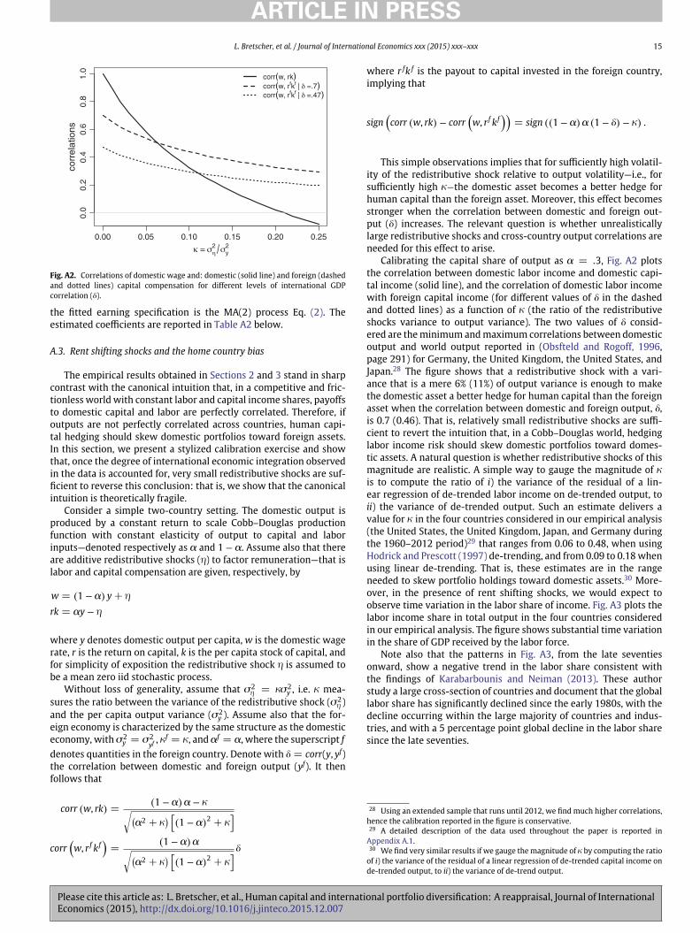
L. Bretscher, et al. / Journal of International Economics xxx (2015) xxx–xxx 15
ARTICLE IN PRESS
0.00 0.05 0.10 0.15 0.20 0.25
0.0
0.2
0.4
0.6
0.8
1.0
= 2y2
corr
elat
ions
corr(w, rk)corr(w, rfkf | =.7)corr(w, rfkf | =.47)
Fig. A2. Correlations of domestic wage and: domestic (solid line) and foreign (dashedand dotted lines) capital compensation for different levels of international GDPcorrelation (d).
the fitted earning specification is the MA(2) process Eq. (2). Theestimated coefficients are reported in Table A2 below.
A.3. Rent shifting shocks and the home country bias
The empirical results obtained in Sections 2 and 3 stand in sharpcontrast with the canonical intuition that, in a competitive and fric-tionless world with constant labor and capital income shares, payoffsto domestic capital and labor are perfectly correlated. Therefore, ifoutputs are not perfectly correlated across countries, human capi-tal hedging should skew domestic portfolios toward foreign assets.In this section, we present a stylized calibration exercise and showthat, once the degree of international economic integration observedin the data is accounted for, very small redistributive shocks are suf-ficient to reverse this conclusion: that is, we show that the canonicalintuition is theoretically fragile.
Consider a simple two-country setting. The domestic output isproduced by a constant return to scale Cobb–Douglas productionfunction with constant elasticity of output to capital and laborinputs—denoted respectively as a and 1 − a. Assume also that thereare additive redistributive shocks (g) to factor remuneration—that islabor and capital compensation are given, respectively, by
w = (1 − a) y + g
rk = ay − g
where y denotes domestic output per capita, w is the domestic wagerate, r is the return on capital, k is the per capita stock of capital, andfor simplicity of exposition the redistributive shock g is assumed tobe a mean zero iid stochastic process.
Without loss of generality, assume that s2g = js2
y , i.e. j mea-sures the ratio between the variance of the redistributive shock (s2
g )and the per capita output variance (s2
y ). Assume also that the for-eign economy is characterized by the same structure as the domesticeconomy, with s2
y = s2yf , jf = j, and af = a, where the superscript f
denotes quantities in the foreign country. Denote with d = corr(y, yf)the correlation between domestic and foreign output (yf). It thenfollows that
corr (w, rk) =(1 − a)a − j√(
a2 + j) [
(1 − a)2 + j
]
corr(
w, rf kf)
=(1 − a)a√(
a2 + j) [
(1 − a)2 + j
]d
where r fk f is the payout to capital invested in the foreign country,implying that
sign(
corr (w, rk) − corr(
w, rf kf))
= sign ((1 − a)a (1 − d) − j) .
This simple observations implies that for sufficiently high volatil-ity of the redistributive shock relative to output volatility—i.e., forsufficiently high j−the domestic asset becomes a better hedge forhuman capital than the foreign asset. Moreover, this effect becomesstronger when the correlation between domestic and foreign out-put (d) increases. The relevant question is whether unrealisticallylarge redistributive shocks and cross-country output correlations areneeded for this effect to arise.
Calibrating the capital share of output as a = .3, Fig. A2 plotsthe correlation between domestic labor income and domestic capi-tal income (solid line), and the correlation of domestic labor incomewith foreign capital income (for different values of d in the dashedand dotted lines) as a function of j (the ratio of the redistributiveshocks variance to output variance). The two values of d consid-ered are the minimum and maximum correlations between domesticoutput and world output reported in (Obsfteld and Rogoff, 1996,page 291) for Germany, the United Kingdom, the United States, andJapan.28 The figure shows that a redistributive shock with a vari-ance that is a mere 6% (11%) of output variance is enough to makethe domestic asset a better hedge for human capital than the foreignasset when the correlation between domestic and foreign output, d,is 0.7 (0.46). That is, relatively small redistributive shocks are suffi-cient to revert the intuition that, in a Cobb–Douglas world, hedginglabor income risk should skew domestic portfolios toward domes-tic assets. A natural question is whether redistributive shocks of thismagnitude are realistic. A simple way to gauge the magnitude of jis to compute the ratio of i) the variance of the residual of a lin-ear regression of de-trended labor income on de-trended output, toii) the variance of de-trended output. Such an estimate delivers avalue for j in the four countries considered in our empirical analysis(the United States, the United Kingdom, Japan, and Germany duringthe 1960–2012 period)29 that ranges from 0.06 to 0.48, when usingHodrick and Prescott (1997) de-trending, and from 0.09 to 0.18 whenusing linear de-trending. That is, these estimates are in the rangeneeded to skew portfolio holdings toward domestic assets.30 More-over, in the presence of rent shifting shocks, we would expect toobserve time variation in the labor share of income. Fig. A3 plots thelabor income share in total output in the four countries consideredin our empirical analysis. The figure shows substantial time variationin the share of GDP received by the labor force.
Note also that the patterns in Fig. A3, from the late seventiesonward, show a negative trend in the labor share consistent withthe findings of Karabarbounis and Neiman (2013). These authorstudy a large cross-section of countries and document that the globallabor share has significantly declined since the early 1980s, with thedecline occurring within the large majority of countries and indus-tries, and with a 5 percentage point global decline in the labor sharesince the late seventies.
28 Using an extended sample that runs until 2012, we find much higher correlations,hence the calibration reported in the figure is conservative.29 A detailed description of the data used throughout the paper is reported in
Appendix A.1.30 We find very similar results if we gauge the magnitude of j by computing the ratio
of i) the variance of the residual of a linear regression of de-trended capital income onde-trended output, to ii) the variance of de-trend output.
Please cite this article as: L. Bretscher, et al., Human capital and international portfolio diversification: A reappraisal, Journal of InternationalEconomics (2015), http://dx.doi.org/10.1016/j.jinteco.2015.12.007

16 L. Bretscher, et al. / Journal of International Economics xxx (2015) xxx–xxx
ARTICLE IN PRESS
1960 1970 1980 1990 2000 2010
0.7
Year
Labo
r In
com
e/G
DP
(%
)
GermanyJapanUKUSA
0.3
0.4
0.5
0.6
Fig. A3. Labor share of income in Germany, Japan, UK and USA
A.4. Cointegration analysis
In this Appendix, we provide a battery of econometric tests onthe time series properties of labor and capital income in the fourcountries in our sample.
Since both the Augmented Dickey–Fuller (Dickey and Fuller,1981) and the Phillips–Perron (Phillips and Perron, 1988) tests can-not reject the null hypothesis of unit roots in labor and capitalincome (results not reported but available upon request), we inves-tigate whether the logarithm of labor income shares a common
Table A3Johansen cointegration test.
Country Number of Trace Max Likelihoodlags Eigenvalue ratio
Germany 0 20.22(0.009)
19.80(0.006)
15.32(0.002)
1 11.377(0.190)
9.504(0.272)
7.196(0.007)
2 10.159(0.302)
8.59(0.370)
6.39(0.012)
3 10.48(0.270)
8.34(0.396)
5.49(0.019)
Japan 0 54.96(0.001)
51.84(0.001)
4.36(0.037)
1 27.42(0.001)
22.86(0.002)
3.70(0.055)
2 17.40(0.026)
12.06(0.109)
4.37(0.037)
3 30.04(0.001)
26.04(0.01)
19.83(0.000)
United Kingdom 0 18.63(0.016)
17.46(0.015)
13.58(0.000)
1 12.41(0.0139)
9.91(0.229)
4.98(0.026)
2 11.30(0.194)
8.39(0.391)
5.23(0.022)
3 12.30(0.143)
10.48(0.183)
7.62(0.006)
United States 0 16.53(0.035)
15.85(0.028)
12.96(0.000)
1 12.28(0.144)
10.61(0.175)
8.76(0.003)
2 13.43(0.100)
8.88(0.339)
3.87(0.049)
3 15.53(0.049)
10.53(0.180)
5.51(0.019)
Note: Johansen cointegration test. The null hypothesis is no pairwise cointegrationbetween labor income and capital income within each country. We report the traceand maximum eigenvalue test statistics for different lag specifications of the first dif-ferenced terms. The last column tests the restriction that the log ratio of labor incometo capital income is stationary, i.e., the log of labor income and the log of capitalincome are cointegrated with cointegrating vector [1, −1] . We report the p-value ofthe test statistics in parentheses.
stochastic trend with the logarithm of capital income, thus imply-ing the existence of a pairwise cointegration relationship within eachcountry.
Table A3 presents econometric evidence based on the Johansencointegration test (Johansen, 1995), in which we allow for a lineardeterministic trend in the data and an intercept (but not a trend) inthe cointegration vector. For each country, the table reports both thetrace statistics and the maximum eigenvalue statistics for differentlags specifications of the first differenced terms. The last column ofTable A3 tests the restriction that the log ratio of labor income tocapital income is stationary, i.e., the log of labor income and the logof capital income are cointegrated with cointegrating vector [1, −1].
The null hypothesis of no cointegration between labor and capitalincome cannot be generally rejected at standard significance levelsfor all countries but Japan. Hence, the long-run restriction suggestedby Baxter and Jermann (1997) of pairwise cointegration within coun-tries is not supported by the data unless the number of lags in thetest equation is zero. The sensitivity of the result to the lag specifica-tion can be due to the low power of the cointegration test, stemmingperhaps from a small sample size.
In Fig. A1 we plot the log ratio of labor income to capital incomein the four countries in our sample. Simple visual inspection suggeststhat the behavior of the log ratio of labor income to capital incomeis not stationary. Indeed, as reported in the last column of Table A3,a formal testing procedure based on the Johansen cointegrating teststrongly rejects the cointegration restriction for all countries.
We acknowledge that if labor and capital income are allowed tohave independent trends, then the ratio of labor income to capitalincome either will grow without bound or approach zero asymp-totically. Therefore, labor’s share will approach one or zero withprobability one. However, it is important to realize that the cointe-gration tests are simply rejecting the hypothesis about the existenceof a pairwise cointegration relationship within each country, but arecompletely silent about the existence of a long-run equilibrium rela-tionship across countries. Moreover, since in this paper we do oureconometric analysis in levels, we allow for implicit cointegratingrelationships in the data.
A.5. Robustness of factor returns correlations
This section tests whether the correlation of the factor returnspresented in Table 8 are sensitive to the way we construct our dataseries on labor income. As mentioned in Appendix A.1, our final dataof labor and capital income stems from two different datasets thatare then combined. An immediate concern is whether the results ofthis paper are robust to the different possible ways of combining thetwo datasets. In particular, one could think of four different waysof combining them: 1) augment the 1960–2003 dataset from 2003onwards (baseline specification); 2) augment the 1960–2003 datasetfrom 1970 onwards; 3) augment the 1970–2012 dataset from 2003backwards; 4) augment the 1970–2012 dataset from 1970 back-wards. We opt for the first alternative for several reasons. First, wechoose to augment the 1960–2003 dataset since this maximizes theoverlap with the data Baxter and Jermann (1997) used in their analy-sis. Second, we decide to splice the datasets in the year 2003 because,at that time, Germany had already reunified, and consequently thedata definitions are consistent across countries. Nevertheless, weexplore the robustness of our results by comparing them for the fourdifferent alternatives.
In Table A4, we recalculate Table 8 for the four alternatives. Theresults for alternatives 1) to 4) are reported clockwise, with the topleft part being identical to Table A5—our baseline specification. Theresults suggest that, keeping the year in which we splice fixed, thereis essentially no difference in the correlations whether we extendthe 1960–2003 or the 1970–2012 dataset. This can be seen from
Please cite this article as: L. Bretscher, et al., Human capital and international portfolio diversification: A reappraisal, Journal of InternationalEconomics (2015), http://dx.doi.org/10.1016/j.jinteco.2015.12.007

L. Bretscher, et al. / Journal of International Economics xxx (2015) xxx–xxx 17
ARTICLE IN PRESS
Table A4Correlation of factor returns using stock market data.
1) Augment 1960–2003 from 2003 onwards 2) Augment 1960–2003 from 1970 onwards
rGL rJ
L rUKL rUSA
L rGL rJ
L rUKL rUSA
L
rGK 0.118
[−0.08,0.24]0.138
[−0.8,0.24]0.110
[−0.07,0.26]0.145
[−0.04,0.27]rG
K 0.033[−0.14,0.20]
0.133[−0.05,0.24]
0.097[−0.06,0.24]
0.154[−0.01,0.26]
rJK 0.122
[−0.05,0.21]0.071
[−0.09,0.19]0.145
[−0.02,0.23]0.194
[0.03,0.26]rJ
K 0.150[−0.05,0.32]
0.167[−0.07,0.28]
0.060[−0.12,0.25]
0.178[−0.02,0.32]
rUKK 0.130
[−0.09,0.26]0.105
[−0.12,0.23]0.101
[−0.10,0.27]0.149
[−0.06,0.29]rUK
K −0.101[−0.22,0.10]
−0.016[−0.15,0.16]
0.138[−0.07,0.22]
0.169[−0.04,0.23]
rUSAFF 0.000
[−0.14,0.11]−0.088
[−0.20,0.04]0.031
[−0.10,0.15]0.041
[−0.10,0.14]rUSA
FF 0.021[−0.13,0.15]
−0.00[−0.16,0.10]
−0.069[−0.18,0.09]
−0.033[−0.16,0.11]
rUSADJ −0.017
[−0.18,0.12]−0.147
[−0.27,0.01]0.035
[−0.07,0.21]0.006
[−0.10,0.18]rUSA
DJ 0.069[−0.16,0.18]
0.014[−0.21,0.13]
−0.045[−0.18,0.15]
−0.017[−0.17,0.16]
rUSASP 0.026
[−0.11,0.12]−0.076
[−0.19,0.05]0.075
[−0.05,0.17]0.070
[−0.06,0.16]rUSA
SP 0.057[−0.12,0.15]
0.027[−0.15,0.12]
−0.046[−0.16,0.11]
−0.015[−0.14,0.12]
3) Augment 1970–2012 from 2003 backwards 4) Augment 1970–2012 from 1970 backwards
rGL rJ
L rUKL rUSA
L rGL rJ
L rUKL rUSA
L
rGK 0.118
[−0.08,0.23]0.138
[−0.08,0.24]0.110
[−0.07,0.26]0.145
[−0.04,0.26]rG
K 0.033[−0.14,0.20]
0.133[−0.05,0.32]
0.097[−0.22,0.10]
0.154[−0.14,0.13]
rJK 0.0123
[−0.05,0.21]0.071
[−0.09,0.19]0.145
[−0.02,0.23]0.195
[0.03,0.26]rJ
K 0.150[−0.06,0.24]
0.168[−0.07,0.28]
0.060[−0.12,0.25]
0.178[−0.02,0.32]
rUKK 0.128
[−0.09,0.26]0.105
[−0.12,0.23]0.099
[−0.10,0.27]0.147
[−0.06,0.29]rUK
K −0.010[−0.22,0.10]
−0.016[−0.15,0.16]
0.137[−0.07,0.22]
0.169[−0.04,0.23]
rUSAFF −0.001
[−0.14,0.11]−0.088
[−0.20,0.04]0.029
[−0.10,0.15]0.039
[−0.10,0.14]rUSA
FF 0.022[−0.14,13]
−0.000[−0.16,0.10]
−0.069[−0.19,0.08]
−0.033[−0.17,0.10]
rUSADJ −0.019
[−0.18,0.12]−0.147
[−0.27,0.01]0.087
[−0.07,0.21]0.058
[−0.10,0.18]rUSA
DJ 0.070[−0.16,0.18]
0.014[−0.21,0.13]
−0.045[−0.18,0.15]
−0.017[−0.17,0.16]
rUSASP 0.024
[−0.11,0.12]−0.076
[−0.19,0.05]0.073
[−0.06,0.17]0.068
[−0.07,0.16]rUSA
SP 0.058[−0.12,0.15]
0.027[−0.15,0.12]
−0.047[−0.16,0.11]
−0.016[−0.14,0.12]
Note: Correlations of human capital returns with physical capital returns. Returns to human capital are estimated using a VAR specification in levels withtwo lags. Returns on physical capital are computed using stock market data (CDAX for Germany, Nikko Securities Composite for Japan, FTSE All-ShareIndex for the United Kingdom, and Fama and French (FF), S&P 500 Total Return Index (SP), and Dow Jones Industrials Total Return Index (DJ) for theUnited States). We report in brackets the 95% confidence interval constructed using sampling-with-replacement raw residuals bootstrap based on 10,000replications.
comparing the correlations vertically across tables. From a horizon-tal comparison across tables, however, one can see that the choiceof the year in which we splice the datasets matters to some extent.Nevertheless, the main result of the table, remain unchanged: U.S.labor income returns innovations are always more correlated withforeign, rather than domestic, stock market returns (this is the keyelement for calibrating our buffer stock saving model).
Table A5Value-weighted diversified portfolio with complete markets.
Shares in each country traded asset:
Investor nationality: Germany Japan U.K. U.S.
Panel A: rk measured from VAR and national accountsGermany −0.225
[−0.76,0.55]0.060
−0.28,0.31]1.576
[0.64,2.16]−0.411
[−1.21,0.62]
Japan 0.742[−0.19,1.76]
−0.606[−1.08,−0.21]
1.882[0.63,2.84]
−1.017[−2.22,0.51]
UK 0.230[−0.56,1.17]
1.059[0.53,1.34]
1.191[−0.08,2.02]
−1.480[−2.50,0.08]
USA 0.019[−0.52,0.91]
0.054[0.11,0.78]
0.786[−0.30,1.41]
−0.341[−1.23,0.87]
Panel B: rk measured using stock market returnsGermany 0.040
[0.04,0.05]0.289
[0.28,0.29]0.145
[0.14,0.16]0.526
[0.51,0.53]
Japan 0.034[0.03,0.04]
0.290[0.28,0.29]
0.139[0.13,0.15]
0.537[0.52,0.54]
UK 0.039[0.03,0.05]
0.287[0.28,0.29]
0.147[0.14,0.17]
0.527[0.5,0.53]
USA 0.039[0.03,0.05]
0.287[0.28,0.29]
0.145[0.14,0.17]
0.530[0.51,0.54]
World share 0.043 0.293 0.150 0.516
Note: Diversified portfolio using stock market returns (CDAX for Germany, NikkoSecurities Composite for Japan, FTSE All-Share Index for the United Kingdom, andFama and French for the United States). Each cell displays the net demand by a resi-dent of country j for the assets of country k expressed as a fraction of home country(country j) marketable assets. We report in brackets the 95% confidence interval con-structed using sampling-with-replacement raw residuals bootstrap based on 10,000replications.
A.6. Hedging human capital in a frictionless complete market
The correlation structure between physical and human capi-tal returns reported in Table 7 is not sufficient to identify thehedging behaviour without additional assumptions on the structureof the economy. In the main body of the paper, we provide a modelof human capital hedging that accounts for both idiosyncratic andaggregate labor income risk, as well as liquidity constraints and mar-ket incompleteness. But in this subsection, we want to show thatthe VAR misspecification is the main driver behind the empiricalresults on human capital hedging reported in the previous literature.Moreover, we want to show that the estimates are characterizedby substantial uncertainty, making the conclusion of human capitalpushing toward overinvestment in foreign assets very far fetched. Toshow this, we now assume—only for this sub-section—that the setof international risky financial assets provides perfect spanning forhuman capital as in Bottazzi et al., 1996; Baxter and Jermann 1997.In other words, we assume that there exists a linear combination ofdomestic and foreign marketable assets that is perfectly correlatedwith the return to domestic human capital returns.
Assuming complete spanning of human capital returns by thestock market returns (as in Bottazzi et al., 1996; Baxter and Jermann,1997), one can compute hedge portfolios for human capital risk viasimple linear projection. Each hedge portfolio is chosen such that ithedges $ 1.00 of human capital income flow. Let hjk be the weight ofthe risky financial asset of country k in the hedge portfolio of countryj residents. The hedge portfolio of country j, hj := [hj1, hj2, . . . , hjK]
′,
is given given by
hj = S−1Yj (A1)
where S is the K × K covariance matrix of returns on risky financialassets in the world portfolio, and Yj is the K ×1 vector of covariancesof financial assets returns with the human capital return of countryj. Notice that since the hedge portfolio is constructed to hedge $ 1.00
Please cite this article as: L. Bretscher, et al., Human capital and international portfolio diversification: A reappraisal, Journal of InternationalEconomics (2015), http://dx.doi.org/10.1016/j.jinteco.2015.12.007

18 L. Bretscher, et al. / Journal of International Economics xxx (2015) xxx–xxx
ARTICLE IN PRESS
1960 1970 1980 1990 2000 2010
0.8
Germany
1960 1970 1980 1990 2000 2010
0.8
Japan
1960 1970 1980 1990 2000 2010
0.8
UK
1960 1970 1980 1990 2000 2010
0.8
USA−0.
40.
00.
4
−0.
40.
00.
4
−0.
40.
00.
4
0.4
0.0
−0.
4
Fig. A4. Log ratio of labor income to capital income in Germany, Japan, the United Kingdom, and the United States.
of human capital, there is no reason for the portfolio weights to addto one.
Moreover, under the complete spanning assumption, one can alsocompute optimal portfolios following the value-weighted approachused in Baxter and Jermann (1997). The value-weighted portfolioapproach, without considering the human capital hedging for themoment, follows from the two funds separation theorem (Merton,1973): in a frictionless one-period economy with no asymmetricinformation, in the presence of K financial risky assets and a risk-freeasset, all individuals will hold a portfolio given by a linear com-bination of the risk free asset and the market portfolio—i.e., thevalue-weighted portfolio. As a consequence, the risky part of eachindividual’s portfolio will have a composition identical to the marketportfolio. The extension of this approach to our international frame-work is straightforward: in equilibrium each investor, independentof his nationality, will hold a risky portfolio with a composition iden-tical to the world portfolio of risky financial assets, i.e., each country’sasset will be in the portfolio with a share equal to the share of thecountry in the world portfolio of marketable risky assets. That is,denoting with pk the fraction of country k risky marketable asset inthe world portfolio, we have that in the absence of human capitalrisk, pk would be the share of country k asset in the portfolio of riskyfinancial assets of each country.
In the presence of non-marketable human capital, portfolio hold-ings will be adjusted due to the hedging motive. Therefore, the
portfolio of risky assets held by a country j individual will dependalso on the covariance of domestic returns to human capital and(domestic and foreign) returns to physical capital. In particular, tohedge the human capital risk, the net demand by a resident ofcountry j for the asset of country k expressed as a fraction of thehome country (country j) portfolio of financial assets will be
pk
[1 +
1 − aj
aj
( 4∑k=1
hjk
)]− 1 − aj
ajhjk, (A2)
where 1 − aj is the labor share of income in country j.The last term in Eq. (A2) is the share of country k marketable
asset that has to be sold to hedge the human capital risk in country j.The expression multiplying pk reflects the funds generated by sellingthe investor’s endowment of the claim to domestic physical capitaland the portfolio that hedges the risks associated with human capitalwealth, i.e.,
1−ajaj
(∑4k=1 hjk
).
The value weighted optimal portfolios implied by the correlationsbetween human and physical capital returns in Table 8 are reportedin Table A5. Panel A focuses on the VAR and national accounts basedestimates of physical capital returns, while panel B use stock marketindex returns.
Panel A shows that, after correcting the VAR misspecification,the Baxter and Jermann (1997) value-weighted approach leads to
Please cite this article as: L. Bretscher, et al., Human capital and international portfolio diversification: A reappraisal, Journal of InternationalEconomics (2015), http://dx.doi.org/10.1016/j.jinteco.2015.12.007

L. Bretscher, et al. / Journal of International Economics xxx (2015) xxx–xxx 19
ARTICLE IN PRESS
inconclusive results concerning the role of human capital for optimalportfolio diversification: large home bias is basically as likely as largeshorting of the domestic market.
Comparing the optimal in portfolios in panel B with the (rescaledto sum up to one) world shares (pk) of the various countries’ stockmarkets in the world market capitalization reported in the last row,the table shows that the inclusion of human capital hedging motivehas basically no effect when the space of tradable claims to capital isthe one of publicly traded companies.
References
Abowd, J.M., 1989. The effect of wage bargains on the stock market value of the firm.Am. Econ. Rev. 79 (4), 774–800.
Alesina, A., Rodrik, D., 1994. Distributive politics and economic growth. Q. J. Econ. 109(2), 465–490.
Attanasio, O.P., Goldberg, P.K., Kyriazidou, Ekaterini, 2008. Credit constraints in themarket for consumer durables: evidence from micro data on car loans. Int. Econ.Rev. 49 (2), 401–436.
Baxter, M., Jermann, U.J., 1997. The international diversification puzzle is worse thanyou think. Am. Econ. Rev. 87 (1), 170–180.
Baxter, M., Jermann, U.J., King, R.G., 1998. Nontraded goods, nontraded factors, andinternational non-diversification. J. Int. Econ. 44 (2), 211–229.
Bertola, G., 1993. Factor shares and savings in endogenous growth. Am. Econ. Rev. 83(5), 1184–1198.
Bhamra, H., Coeurdacier, N., Guibaud, S., 2014. A dynamic equilibrium model ofimperfectly integrated financial markets. J. Econ. Theory 154, 490–542.
Bottazzi, L., Pesenti, P., van Wincoop, E., 1996. Wages, profits and the internationalportfolio puzzle. Eur. Econ. Rev. 40 (2), 219–254.
Brainard, W.C., Tobin, J., 1992. On the internationalization of portfolios. Oxf. Econ. Pap.44 (4), 533–565.
Brunnermeier, M.K., Julliard, C., 2008. Money illusion and housing frenzies. Rev.Financ. Stud. 21 (1), 135–180.
Campbell, J.Y., 1996. Understanding risk and return. J. Polit. Econ. 104 (2), 298–345.Campbell, J.Y., Shiller, R.J., 1988. The dividend–price ratio and expectations of future
dividends and discount factors. Rev. Financ. Stud. 1 (3), 195–228.Campbell, J.Y., Vuolteenaho, T., 2004. Inflation illusion and stock prices. Am. Econ. Rev.
Pap. Proc. 94 (2), 19–23.Carroll, C.D., 1992. The buffer stock theory of saving: some macroeconomic evidence.
Brook. Pap. Econ. Act. 23 (2), 61–135.Carroll, C.D., 1997. Buffer stock saving and the life cycle/permanent income hypothe-
sis. Q. J. Econ. 112 (1), 1–55.Carroll, C.D., 2004. Theoretical foundations of buffer stock saving. Johns Hopkins
University manuscript.Carroll, C.D., 2009. Precautionary saving and the marginal propensity to consume out
of permanent income. J. Monet. Econ. 56 (6), 780–790.Coeurdacier, N., 2009. Do trade costs in goods market lead to home bias in equities?. J.
Int. Econ. 77 (1), 86–100.Coeurdacier, N., Kollmann, R., Martin, P., 2013. International portfolios, capital accu-
mulation and foreign assets dynamics. J. Int. Econ. 80 (1), 100–112.Coeurdacier, N., Rey, H., 2013. Home bias in open economy financial macroeconomics.
J. Econ. Lit. 51 (1), 63–115.Cole, H., Obstfeld, M., 1991. Commodity trade and international risk sharing: how
much do financial markets matter?. J. Monet. Econ. 28 (1), 3–24.Cole, H., 1988. Financial structure and international trade. Int. Econ. Rev. 29 (2),
237–259.Davis, S.J., Willen, P., 2000. Using financial assets to hedge labor income risk: estimat-
ing the benefits. University of Chicago manuscript.Deaton, A., 1991. Saving and liquidity constraints. Econometrica 59 (5), 1121–1142.Deaton, A., Laroque, G., 1992. On the behaviour of comodity prices. Rev. Econ. Stud. 59
(1), 1–23.Dickey, D.A., Fuller, W.A., 1981. Likelihood ratio statistics for autoregressive time series
with a unit root. Econometrica 49 (4), 1057–1071.Efron, B., Tibshirani, R.J., Rubin, Donald.B., 1995. An introduction to the bootstrap.
Chapman and Hall, LondonEldor, R., Pines, D., Schwarz, A., 1988. Home asset preference and productivity shocks.
J. Int. Econ. 25 (1), 165–176.Engel, C., Matsumoto, A., 2009. The international diversification puzzle is not as bad as
you think. Am. Econ. J. Macroecon. 1 (2), 155–188.Fama, E.F., French, K.R., 1992. The cross-section of expected stock returns. J. Financ. 47
(2), 427–465.Fama, E.F., Schwert, W., 1977. Human capital and capital market equilibrium. J. Financ.
Econ. 4 (1), 95–125.Francis, N., Ramey, V.A., 2004. A new measure of hours per capita with implications
for the technology-hours debate. UCSD manuscript.Francis, N., Ramey, V.A., 2009. Measures of per capita hours and their implications for
the technology-hours debate. J. Money Credit Bank. 41 (6), 1071–1097.
French, K.R., Poterba, J.M., 1991. International diversification and international equitymarkets. Am. Econ. Rev. Pap. Proc. 81 (2), 222–226.
Froot, K.A., Obstfeld, M., 1991. Intrinsic bubbles: the case of stock prices. Am. Econ.Rev. 81 (5), 1189–1214.
Gali, J., 1999. Technology, employment, and the business cycle: do technology shocksexplain aggregate fluctuations?. Am. Econ. Rev. 89 (1), 249–271.
Gelman, A., Carlin, J.B., Stern, Hal.S., Rubin, Donald.B., 1995. Bayesian data analysis.Chapman and Hall, London
Gopinath, G., Kalemli-Özcan, C., Karabarbounis, L., Villegas-Sanchez, C., 2015. Capitalallocation and productivity in south europe. Harvard University manuscript.
Gourinchas, P.O., Parker, J.A., 2002. Consumption over the lifecycle. Econometrica 70(1), 47–89.
Grauer, R.R., Hakansson, N.H., 1987. Gains from international diversification:1968–1985 returns on portfolios of stocks and bonds. J. Financ. 42 (3), 721–739.
Haliassos, M., Michaelides, A., 2002. Calibration and computation of household port-folio models. In: Guiso, Luigi, Haliassos, Michael, Japelli, Tullio (Eds.), HouseholdPortfolios. MIT Press, Cambridge.
Hau, H., Rey, H., 2006. Exchange rates, equity prices and capital flows. Rev. Financ.Stud. 19 (1), 273–317.
Heathcote, J., Perri, F., 2013. The international diversification puzzle is not as bad asyou think. J. Polit. Econ. 121 (6), 1108–1159.
Heaton, J., Lucas, D., 1997. Market frictions, saving behaviour, and portfolio choice.Macroecon. Dyn. 1 (1), 76–101.
Hodrick, R.J., Prescott, E.C., 1997, February. Postwar U.S. business cycles: an empiricalinvestigation. J. Money, Credit, Bank. 29 (1), 1–16.
Iacoviello, M., 2005. House prices, borrowing constraints, and monetary policy in thebusiness cycle. Am. Econ. Rev. 95 (3), 739–764.
Jappelli, T., Julliard, C., Pagano, M., 2001. Italian households’ portfolio diversification.. XIX Rapporto Sul Risparmio e Sui Risparmiatori in ItaliaBNL/Centro Einaudi, pp.91–121.
Johansen, S., 1995. Likelihood-based Inference in Cointegrated Vector AutoregressiveModels. Oxford University Press, Oxford
Karabarbounis, L., Neiman, B., 2013. The global decline of the labor share. Q. J. Econ.129 (1), 61–103.
Kim, J., 1994. Bayesian asymptotic theory in a time series model with a possiblenonstationary process. Econ. Theory 10 (3), 764–773.
Kollmann, R., 2006. International portfolio equilibrium and the current account. CEPRdiscussion papers 5512.
Lustig, H., Nieuwerburgh, S.V., 2008. The returns on human capital: good news on WallStreet is bad news on main street. Rev. Financ. Stud. 21 (5), 2097–2137.
MaCurdy, T.E., 1982. The use of time series processes to model the error structure ofearnings in a longitudinal data analysis. J. Econ. 18 (1), 83–114.
Merton, R.C., 1973. An intertemporal capital asset pricing model. Econometrica 41 (5),867–886.
Michaelides, A., 2003. International portfolio choice, liquidity constraints and thehome equity bias puzzle. J. Econ. Dyn. Control. 28 (3), 555–594.
Obsfteld, M., 1994. Risk-taking, global diversification, and growth. Am. Econ. Rev. 84(5), 1310–1329.
Obsfteld, M., Rogoff, K., 1996. Foundations of international macroeconomics. Cam-bridge: MIT Press
Obstfeld, M., Rogoff, K., 2001. The six major puzzles in international macroeconomics:is there a common cause?. In: Bernanke, Ben.S., Rogoff, Kenneth (Eds.), 2000NBER Macroeconomics Annual. MIT Press,
Oxley, L., McAleer, M., 1993. Econometric issues in macroeconomic models withgenerated regressors. Econometrica 7 (1), 1–40.
Palacios-Huerta, I., 2001. The human capital of stockholders and the internationaldiversification puzzle. J. Int. Econ. 54 (2), 309–331.
Pesenti, P., van Wincoop, E., 2002. Can nontradables generate substantial home bias?.Journal of Money, Credit, and Banking 34 (1), 25–50.
Phillips, P.C.B., Perron, P., 1988. Testing for a unit root in time series regression.Biometrika 75 (2), 335–346.
Piketty, T., 2014. Capital in the Twenty-first Century. Harvard University Press.Rotemberg, J.J., 2003. Stochastic technical progress, smooth trends and nearly distinct
business cycles. Am. Econ. Rev. 93 (5), 1543–1559.Santa-Clara, P., Valkanov, R., 2003. The presidential puzzle: political cycles and the
stock market. J. Monet. Econ. 58 (5), 1841–1872.Schervish, M.J., 1995. Theory of Statistics. Springer Series in Statistics, Springer, New
YorkSerrat, A., 2001. A dynamic equilibrium model of international portfolio holdings.
Econometrica 69 (6), 1467–1489.Stockman, A.C., Dellas, H., 1989. International portfolio nondiversification and
exchange rate variability. J. Int. Econ. 26 (3), 271–289.Szeidl, A., 2013. Stable invariant distribution in buffer-stock savings and stochastic
growth models. Central European University manuscript.Tesar, L.L., 1993. International risk-sharing and nontraded goods. J. Int. Econ. 35 (1),
69–89.Van Nieuwerburgh, S., Veldkamp, L., 2009. Information immobility and the home bias
puzzle. J. Financ. 64 (3), 1187–1215.Zeldes, S.P., 1989. Consumption and liquidity constraints: an empirical investigation.
J. Polit. Econ. 97 (2), 305–346.
Please cite this article as: L. Bretscher, et al., Human capital and international portfolio diversification: A reappraisal, Journal of InternationalEconomics (2015), http://dx.doi.org/10.1016/j.jinteco.2015.12.007