b

LA-UR- 94.1750v

Tii:

Author(s):

Su6nM9d to.

LosAlamosNATIONAL LABORATORY

An Analysis of Three Nuclear Events in P-Tunnel

William Fourney, University of MarylandRichard DiclG University of MarylandSteven R. Taylor, LANL, Group EES-3, GeophysicsThomas N. Weaver, LANL, Group EES-3, Geophysics

.

Milestone Report

I H415 Program

DISTRIBUTION OF THIS DOCUMENT ISUNLIM~

LooAlamoa Nationalbbomtory, WI alflrnutiva action/aqu81opprturrtty●nrpldyar,la OPOMladby the LMvomlty of Cdltornia Ior tho US, Dapamnant of Enargyundw mntmct w-74Q$ENG46. By aocaptana ofthk!wtkk W LnMbbf MCW@ZOOtit ~ U.S tivofnmant mtdns ● ~no~dudvg, mYWfMO ~nw top#Miahor mprodua tha @iahad form d M. contribution,or to●nowothomtodo 00, for U.S. Qovernmantpurpoaos.The Los Alumos National Laboratory~~ti_WW*m*~U**_Oft*U.s Xfi~~ntofEnefo,

Form NO 030 R5ST Z6291OI9I

AN ANALYSIS OF THREE NUCLEi4 R EVENTS IN P-TUNNEL

WILLIAM L. FOURNEY, RICHARD D. DICK STEVEN R. TAYLOR

AND THOMAS A. WEAVER

GEOPHYSICS GROUP EES-3

LOS ALAMOS NATIONAL LABORATORY

May 3, 1994

) 74-LAUR-94-3E?EZ2E

INSCLAIMER

Thisreportwasprepared M an account of work sponsored%y an agency of the United StatesGovernment. Neither the United States Government nor any agency thereof, nor arw of theiremployees, makes any warranty, expreaa or implied, or asaurnca-any legal liability or rcqronsi-bility for the accuracy, eomplctertcas,or usefulnessof any information, apparatus, product, orprocess ditched, or represents that ita use would not infringe privately owned rights. Refer-ence herein !O any specific commercial product, process,or service by trade name, trademark,manufacturer, er otherwise does not necessarily constitute or imply ita endorsement, recom-mendation, or favoring by tbe United Stata Government or any agency thereof. The views●nd opinions of autho~ -.preaccd herein do not necessarily state or reflect those of theUnited Statca Government or any ●gency thereof,

~hslk’

DISTRIBUTION OF THISDoCUMENT IS UNLIM~

r

ABSTRACT

This report examines experimental results obtained from three P Tunnel events - Mission Cyber,

Disko Elm, and Distant Zenith. The objective of the study was to determine if there were any

differences in the explosive source coupling for the three events. It was felt that Mission Cyber

might not have coupled well because the ground motions recorded for that event were much lower

than expected based on experience from N Tunnel. Detailed examination of the physical and

chemical properties of the tuff in the vicinity of each explosion indicated only minor differences. In

general, the core samples are strong and competent out to at least 60 m from each working point.

Qualitative measures of core sample strength indicate that the strength of the tuff near Mission Cyber

may be greater than indicated by results of static testing. Slight differences in mineralogic content

and saturation of the Mission Cyber tuff were noted relative to the other two tests, but probably

would not result in large differences in ground motions. Examination of scaled free-field stress and

acceleration records collected by Sandia National Laboratory (SNL) indicated that Disko Elm

showed the least scatter and Distant Zenith the most scatter. Mission Cyber measurements tend to

lie slightly below those of Distant Zenith, but still within two standard deviations. Analysis of

regional seismic data from networks operated by Lawrence Liverrnore National Laboratory (LLNL)

and SNL also show no evidence of Mission Cybm coupling low relative to the other two events.

The overall conclusion drawn from the study is that there were no basic differences in the way that

the explosions coupled to the rock.

1.0 Introduction

Three instrumented nuclear tests, Mission Cyber, Disko Elm, and Distant Zenith, were

conducted in the P-Tunnel complex within the past six years. Sandia National Laboratories (SIW)

measured stress and acceleration for all three events at scaled ranges of 4 to 170 tit l/q horizontally

from the source. In addition, Lawrence Livermore National Laboratory (LLNL) and SNL recorded

the far-field ground motion at several stations on their seismic networks. The study documented in

this repofi was motivated because of the presumed anomalous ground motion results from Mission

Cyber compared to Disko Elm and other N-Tunnel events. The belief was based on interpretations

of the measured ground motion values that the Mission Cyber source coupled poorly to the medium.

The values measured were lower [Bass, 1975] than ground motion predictions based on N-Tunnel

tuff property data. To the contrary, the measured ground motion from Disko Elm (conducted after

Mission Cyber) agreed with predictions using N-Tunnel tuff properties.

Our approach to the study included an examination of the core and

obtained from rock at the three event sites, an analysis of the close-in

2

physical property data

gage data (stress and,1 :.

acceleration) from all the P-Turme! tests, and an analysis of the seismic data collected by LLNL and

SNL. This report is organized into five sections. After this brief introduction, Section 2 presents

results of an examination of the core, a brief review of tuff properties, and the mineralogy of the

tuff. Section 3 presents comparisons of the close-in stress and acceleration signals and results of

fast Fourier transform (ITT) analysis of the signals. An analysis of the two sets of seismic data for

the three tests is presented in Section 4. Finally conclusions hmed on our interpretation of the

results are presented in Section 5.

Figure 1.1 shows a map of the P-Tunnel complex and the mined drifts for the three tests

[Containment, 1987, 1989, 199 1]. The stratigraphic section for Aqueduct .Mesa and the elevations

for the events are shown in Figure 1.2. As shown in the figure, all three tests were conducted at

approximately the same elevation (1682 m). Mission Cyber, the first test, was conducted in the

u12P.02 drift in sub-unit MC-2 of the Paintbrush tuff (la~l~ Tp in Figure 1.2). Disko Elm. the

second test, was detonated in tt.e U12P.03 drifl in sub-unit MC-3 of the Paintbrush tuff. Distant

Zenith was fired in the U 12P.04 drift in sub-unit MC-O of the Paintbrush tuff. Three vertical

exploratory holes were drilled in Aqueduct Mesa, UE12P#Ol, UE 12P#4, and UE 12P#6, to

characterize the P-Tunnel tuff. These holes are shown in Figure 1.1. Hole UE 12P#4 was very

close to the working point (WP) for Mission Cybcr and provided one of several cores that the

authors viewed at the Core Library maintained by the L’nited States Geological Survey at the

Nevada Test Site (NTS). Figure 1.3 shows an example of the location of the many holes at the

three sites that were cored to evaluate the tuff and then used for emplacement of accelerometer and

stress gages.

2.0 Core analysis and tuff properties

The properties assigned to the working points for the three tests are listed in Table 2.1

[Containment, 1987, 1989, 1991]. As noted, the tuff properties are nearly the same at the different

WP locations although the actual strata for each we~e in different subunits of the Paintbrush tuff. At

the Mission Cyber WP location the material is described as zeolitize.d, bedded ash-fall and reworked

ash-fall tuff and tuffaceous sandstone [Torres, 1988]. The degree of zeolitization is about 65?I0

[Containment, 1987], The Disko Elm WP is characterized [Containment, 1989] as the MC-3

subunit and consists of zeolitized, medium grained, calcalkaline ash “fall tuff with scattered silica

nodules, The Distant Zenith WP, located in the MC-O subunit, is described as massive to partially

reworked, zeolitiz.ed, calcalkaline ash-fall tuff. The degree of zeolitization at the Disko Elm and

Distant Zenith WP locations is greater (nearly twice the amount) than at the .Mission Cyber WP

[Containment, 199 1], Table 2.1 also indicates the mineral

[Containment, ;991]. Disko Elm and Distant Zenith had 60%

3

constituents of the tuff at each WP

c!inoptolite while Mission Cyber had.,.,, ,

.

1

only 33%. The remaining major constituents for Mission CybeI are 16% smectite and 47%

amorphous material. This combination of minerals in the htff is much greater for the Mission Cyber

site than for the other two sites where these constituents amounted to less than 10%. For Disko Elm

and Distant Zenith approximately 35% of the tuff consists of opal, quartz, plagioclase, and k-

feldspar, wide for Mission Cyber these ingredients amount to only 3%. Hence, there are

differences in the mineral content between the tuff at the Mission Cyber WP and the WP for Disko

Elm and Distant Zm.ith.

Table 2.1 Working Point Tufl Charwteriatics

Mis! m Disco&

DistantZ&ni.th

Lcuation

D@ SGZ (m)

TuffstIata

WP Elevation MSL(M)

TuffMalium

Aquahm Mesa Aqueduct Mesa

270.6 261.2 263.8

Paintbrush MC-3 Paintbmsh MC-OPaintbrush MC-2

1682.4 1682.4 1684.4

Zcolitized/Uh-Fall

CalcalkalineReworked Ah-Fall

Tuffaxous SS

MasSNeZdkized

CalcalkakAsh-Fall

MassivePartial Reworkd~tiw

CakatkdineAsh-Fall

Bulk Density Q/cc)

Grain Density (@c)

1.89 1.91

2.45

1.89

2.43 2.44

Watclcontent(% Wd weight) 19.2

37.3

7.3

I8.6

37

96

18,9

36.7

98.4

Porosity (%)

Satumtion (%)

Gas-FilkdPorosity (%) I .4

2771

59

3

1.8

2760

33

1

1.4

3014

60

12

P-Wave Velocity (M/s)

Clinoptilolite (%)

w (%)

@ (%)

Plagioclasc (%)

K-l%ldqxu (%)

Illi!e (%)

Srnectite (%)

Amorphous (’%)

3 J

10 7

20 13

2

5 4

2

16

47

4

We made a qualitative analysis of the core from P-Tunnel to ascertain the quality and

strength of the material throughout the stratigraphic sectior~from both vertical and hc. izontal core.

The core from several holes were examined including UE12P.04, U 12P.02 IH- 1, U 12P.03 IH-2,

and U 12P.04 IH-2 and strength values were assigned in qualitative terms. In general, kioles

designated with an III are horizontal instrument holes, those with a U are vertical holes drilled from

the upper surface of the mesa, and the hole designated by UE was an exploratory horizontal hole

drilled from the tunnel portal prior to the drift being constructed. The core was evaluated according

to the apparent strength of the tuff, the density, the porosity, and the appearance. The rock was

assigned a strength value based on a scale of zero to ten with the zero being assigned to the sandy,

crumbly, weak material and ten assigned to the dense, fine-grained, strongest material. Strength

was estimated by how easy or how hard it was to break material from the core, the presence of fine

grains or coarse grains, the amount of inclusions large and small, and the tone or sound when the

core section was lightly tapped with a metal rod. The density was estimated by hefting sections of

the core and comparing the weights among the various sections examined. The porosity was

evaluated by how quickly the tuff sections absorbed water. Some of the core was examined twice

and some even a third time to establish consistency in ti~e assignment of relative strength.

Calibration of the qualitative strength with measmd strength data was accomplished using Ter;a

Teks values from hole UE 12P.04 for unconfined and triaxial tests Vorres, 1988]. The average

measured sttrength was correlated to an assigned relative strength value of five.

Figure 2.1 is a plot of relative strength versus depth for the vertical exploratory core hole

UE12P.04 which is located very near the Mission Cyber SVP. The plot indicates 18 m of weak cap

rock, then approximately 116 m of strong tuff, followed by 110 m of weak tuff. At the Mission

Cyber WP or the 268 m level and for about 37 m abcve and 24 m below the WP the tuff relative

strength is high (about 7.5 on our scale). There are layers at 18, 225, 29?. m, each about 1.5 m

thick that consist of sandy unconsolidated material which was assigned a relative strength of

between zero and one. The average strength for the entire section is 4.9 and within 60 m of the WP

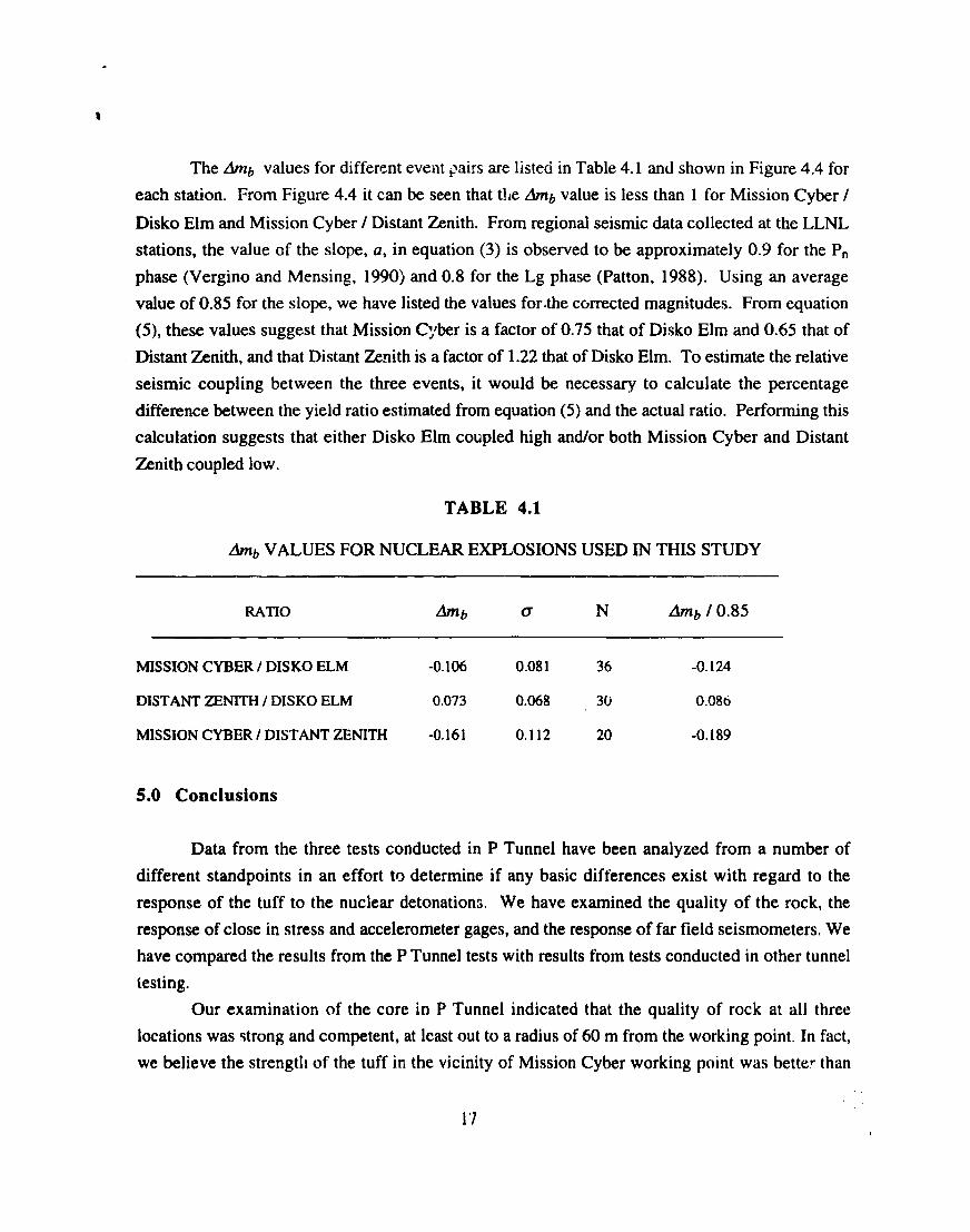
the average relative st.mngth is 5.1. A comparison of relative strength with measured strength is

shown in Figure 2.2. The correlation is very good except in the vicinity of the Mission Cyber WP.

In an effort to see if the difference between the qualitative analysis and ths measure values at the WP

wm a result of the assigned relative strength, this section of core was examined three times on three

separate trips to the Test Site and each time the same relative strength values were assigned.

At this juncture these differences have not been resolved and in our view the tuff in the

vicinity of the WP is strong, competent materiai and hence, good coupling should result. The

measurements by Terra Tek, except for the results from two triaxial

is, the tuff in the vicinity of the working point is relatively weak.

5

test, indicates the opposite, that

This finding should be further

.

1

examined by having additional tests conducted on core from the vicinity of the working point.

Several horizontal core holes were drilled for transducers at the tunnel levels for the three

events in P-Tunnel. An analyses of one of the three holes for Mission Cyber, U i 2P.02 IH- 1 is

shown in Figure 2.3. The tuff had high strength, 5.0 to 7.5, aad was consistent over the length of

the core. A few weaker layers were observed in each of the holes, but not like those observed for

the vertical holes. In addition the tuff within 60 m of the WP was uniform in terms of strength,

porosity, and density based on the horizontal core.

A similar analysis was done for the two Disko Elm horinmal core holes which SNL used as

instrument holes. In hole U12P.03 III-2, the tuff has high strength, 7.0, over the !ength of the core

except for a thin layer at 45.8 m from the collar. Generally, the tuff within 60 m of the WP for

Disko Elm has a relative strength of 7.0 and the quality is consistently good at the tunnel level over

that distance.

A similar analysis was performed for the horizontal inst.iument holes at tunnel level for the

Distant Zenith site. The core from U12P.04 II-I-2indicated good quality tuff with a strength of 6.0

to 7.0 from the WP out to 60 m, similar to that of Mission Cybcr and Disko Elm.

Another horizontal exploratory core hole, U 12P.06 UG-1, was drilled recently and extends

192 m northward from the U12P.01 drift of the P-Tunnel complex. This core was also examined in

a qualitative manner and the results are presented in Figure 2.4. In this hole the tuff quality was

noticeably poorer than in other horizontal holes. As indicated in the figure there are many weak

layers (relative strength 1.0 to 3.0) mixed with intervals of strong material (relative strength 6.0 to

7.0). One weak section 30 m long in the middle of the core had strengths ranging from 0.5 to 3.5.

Other intervals had strength assignments as low as 2.0. The tuff in this horizontal section of P-

Tunnel has low quality, many weak layers, inconsistent strength charactdstics, and highly variable

rock quality in.the surrounding 60 meters from the end of the drill hole. These features coiild affect

the manner in which shock/stress waves propagate [Fourney et a!, 1993] and hence the ground

motion amplitudes would be uirninished.

The characteristics of the tuff in the vicinity of the three events in P-Tunnel based on

examination of the core show many weak layers in combination with strong layers, especially in the

vertical direction. Some of the weak layers are within one wavelength (100 to 150 m) of the stress

wave gen( rated by the source and hence reflections from these layers may be superimposed on the

initial wave. Consequently the structure of the observed wave form may be modified even though

the weak zones may not bin the immediate vicinity of the WP or in the line-of-sight of the gage.

Because of the nature of the strength tests perfo~med by Terra Tek, the specimen material

used for the tests was good, high quality lengths of core. No test specimens were selected from the

weak, sandy, crumbly layers of tuff because this material will not hold together. Hence, the overall

strength data used in the codes and in other interpretive processes may present the tuff as strong

6

.

t

while evidence of the weak zones are missing. In other words there is bias towards a material that

is too strong and does not represent rhe strength variations of the tuff strata.

The tuff characteristics for the three nuclear events are very similar in terms of strength, but

there are some differences. For example, the calculated air-filled void of the tuff for the Mission

Cyber WP is 1.8 % and is 1.4 % at the other two sites. This is a small difference, but could

account for some of the presumed diffemmces in ground motion and stress between Mission Cyber

and Disko Elm and N-Tunnel response. Differences in mineral content at each test site is another

factor. For example, minerals for the tuff at the Disko Elm and Distant Zenith WP are very similar,

but at Mission Cyber the percentages of the major mineral constituents are noticeably different.

Perhaps these differences in mineral content and their possible affect on stress wave coupling

should be examined in more detail.

3.0 Analysis of Ground Motion

3.1 Introduction.

Measurements for P Tunnel Events.

In this section we present an analysis of data taken by scientists from San flia National

Laboratories from Mission Cyber, Disko Elm, and Distant Zenith. The tests were not of the same

yield so whete comparisons m made the results will be compared in scaled form. At times we will

make comparisons of P Tunnel results with results of a similar nature obtained from tests conducted

in N Tunnel.

Sandia fielded both stress gages and accelerometers on all three tests. Velocities and

displacements were obtained by integration of the acceleration data. Gages were placed at scaled

ranges varying from 4 to 170 m/!.tl’3. The smallest number of measurements were made for

Mission Cyber and the largest number of measurements were made for Distant Zenith. We did not

have the results from all of the gages fielded but were able to obtain most of the results from ail

three tests.

3.2 Measured Results.

Figure 3.1 shows records obtained from a representative sample of stress gages fielded by

Sandia cmthe three tests. These results are for measurements of stress in the radid direction. The

gages shown were selected to demonstrate typical scatter and quality that was present in the results

obtained. For example - in Figure 3.1a where results are presented from Mission Cyber - the

results obtained from the gage at 35.6 scaled meters and the results obtained for the gage at 36.4

scaled meters show that the peak magnitude recorded at the slightly closer gage was more than twice

that of gage loca:cd only 0.8 scaled meters away.

Figure 3. lb shows results of stress measurements made from the Disko E!m Event. @n that ,,.:, .

7

particular test, eleven measurements of stress were conducted at ranges from 14.5 scaled metm to

65.3 scaled meters. At two ranges (26.6 scaled meters and 34.2 scaled meters) two separate

readings of radial suess were made at the same location. Excellent agreement wixsobtained between

those two pairs of readings and the resulting points lie almost on top of one another. The result

from gage 46-02 located at 36.2 scaled meters, however, was quite differen+ fr~m the result

obtained from gage 39-U1 located only 2.2 scaled meters away at 33.8 scaled meters.

Disagreement is also evident between g-age46-02 (36.2 scaled meters) and 42-01 (2. 1 scaled meters

away at 38.3 scaled meters). It is not clear which values are correct. Gage 46-0.2 agrees with 46-04

which is at ex tctly :he same location but disagrees greatly with 39-01 (7..2scaled meters closer to

the shot). Gage 42-01 on the other hand agrees with the results from 39-01.

As indicated earlier, Distant Zenith had more instrumentation installed than either Mission

Cyber or Disko Elm. We do not have all of the results but were given a good representative sarnpie.

of both stress and acceleration values. Figure 3. lC gives stress measured as a function of time for a

number of the gages fielded on Distant Zenith. In this case stress records were obtained from a

range of about 7.1 sealed meters to a range of 116.2 scaled meters. Shown in the figure are results

from two gages located at the same location - 35.6 scaled meters from he center of the source.

There was a significant difference between the results obtained for these two gages with one of the

gages reading about twice the amplitude of the second gage. Scientists at Sandia noted the pmence

of faults in the vicinity of both Disko Elm and Distant Zenith. l%e~ attribute some of the differences

to the presence of these faults. In particular the difference in the two gages just mentioned is

attributed to the presenm of such a fauit.

Figure 3.2 shows representative samples of the readings from the accelerometers fielded by

Sandia in the three tests under discussion. These are presented to give an indication of the scatter in

the data and the quality of the data obtained. Notice from the figure that the accelerometer signals

from both Mission Cyber and Distant Zenith are noisy compared to the signals from Disko Elm.

3.2. ) Times of arrival

We examined all of the data from standpoint of arrival times. We looked at both the arrival

time of the first signal and tht+mival time of the peak values. If voids, open joints or layers of

weak materials are present in the in!erval between the gage and the working point then anomalies

should be present in the arrival time of the first signals. If the pulse shapes are different from test to

test or from location to location within the same test, then there should be anomalies in the arrival

times of the peaks. The examination of the arrival times is a good check on assuring proper

identification of the gages. The time of arrival data can also be used to determine wave speed which

serves as a validation of results obtained from sound speed trials.

The result of looking at the time of arrival versus scaled range of the first signal for both,

8

1

stresses and acceleratkms fmrn AUthree tesu indicates that all of the data appears to be we!] behaved

except for the result obtained from gage 3934-01 (a stress gage located at a scaled range of 15.7

rdkixin in Mission Cyber). The arrival tme from this gage was much later than would be expec*-d

based upon tkc gage location and t!! shape of the signai was aJso abnonmd when compared :0 the

ouiput of other gages from the test. This particular gage recorded stress fur 80 milliseconds after

detonation and in addition to the late arrival time the amplitude recorded was only about 0.5 kilobars

- much lower than expected at that range. The conclusion is that this signal should not be included

in further auaiysis.

A least square fit was performed on the data from each of the t?sts. The inverse of the slope

of these lines gives the a~erage velocity of the signal through the tuff. The velocities vary from

2661 m/s for Disko Elm to 30(K)tis for Mission Cyber. The velocity fo, Distant Zenith (2934 mk)

lies very close to the Mission Cyber m’jult. These values are in good agreement with the P wave

speeds detmrnineci from core testing as given i.. Table 2.1.

Since the shape of the stres pulse is very much diffknmt from the shape of the acce]eraticm

pulse we expect a different result for peak arrival times for stress than for acceleration. The

information on @c arrival times versus wled range for acceleration is in good agreement with the

information on first signs! arrival information. A least square fit was found for the results of each

of the three tests and little variation was found from test to test. The wave velocities determined

from the fit ranged from 2740 rds fox Distant Zenith to 2463 mls for Disko Elm. The velocity

determined for Mission Cyber was 2604 m/s. The information on the arrival times versus scaled

range of the peak stnxs values indicated that a number of the points from the Distant Zenith test and

one point from the Mission Cyber test could be suspect. In the Mission Cyber test thu gage closest

tc the source (15.7 scaled meters) had a late arrivaJ time as did all of the Distant Zenith gages located

more than 57 scaled meters from the source. Least squ?,”~ fits to the test iesults indicate that the

velocities vary from 2500 rrks for Disko Elm to 1976 rds for Distant Zenith. The velocity for

Miss!on Cyber was 2330 rnk. Figure 3.3 shows the data points from the Distant Zenith test along

with t!! least.. quare fit irom the Mission Cyber and Disco Elm tests. Notice from the figure that the

last four data points from Distant Zen.kh appear to fit well the slope as determined from the other

two tests but there appears to be a time s$i~t in he peak signals. Such a time delay could be caused

b~’the signal passing an open fault such as reported by Sand ~scientists but these particular gages

were not the ones identified by Saiidia as being g~atly affected by the faults.

Notice frcm Figure 3.3 that there are three other gages (the ones between 50 and 6Gscaled

meters in the figure) that appear shiited later in time but not to such an extent as the gages farther

out. 1 here are also two other gages at similar locations that are below the least square fit line and

therefore have arrival times earlier than those predicted from.the results of Mission Cyber and Disco

Elm events. h was in this area that Sandia scientists noted the presence of faults. For all gages that

9

were time delayed we would expect a decrease in stxess magnitude but this was not the case. Some

of the gages which were located at the same location had stress magnitudes which vaived by factors

of two and yet exhibited the same time delay in the peak signal arrival times.

As a consequence of looking at arrival times the results fmm two of the gages that measured

stmses in the Mission Cyber event am felt to be questionable. The fust of the two suspect gages is

at a scaled distance of 15.7 m, identified as gage 3934-01, which is questiorwd because of a very

late time of arrival of fmt signal. It also happens to haw a very low amplitude compared to the

other gages fielded on t-heevent. The second gage from MissIon Cyber that is questionable is gage

3938-01 which was located at a scaled range of 63.1 meters. It is suspect from the standpoint of a

late arrival time of the peak stress value. At least three and as many as eight of the gages in Distant

Zenith test could be questioned based upon the anival of peak stress data. A similar delay was not

seen in peak acceleration arrival time for companion gages - that is for acceleration gages located in

the same package. Only the one gage from Mission Cyber (3934-01) is dropped from the data base

at this time. The others will be retained but special attention is given to t.keresults when ccmparing

them to the other data.

3.2.2 Stxess magnitudes

Figure 3.4 is a comparison of the stress rnrqytitudes measured in the three P Tunnel events.

Points marked with a” 1” are from Distant Zenith. Those marked with a “2” are Mission Cyber and

the 3’s are from Disko Elm. (This code will be utilized in all figures presented in this report.) The

hew-y solid line in the figure gives the location of plus one starxiard deviation from the mean line for

‘k results of Distant Zenith and Disko Elm. The lower dashed line gives the location of the minus

one standard deviation for the same data sets. The light solid line gives the mean of all of the data

from all three test taken as a data set. The light solid line running through the two open squares

indicates what would be expected from earlier tunnel testing. These results indicate that the data

from Disko Elm has ve~y little scatter and in general seem to be higher than those from the other two

tests. The results from Distant Zenith am scattered with one point falling on the phw one standard

deviation line but with mariy points being lower than the Disko Elm values and a number of points

falling even below the Mission Cyber results. The results from Mission Cyber show little scatter

but all points fall on the lower edge of the scatter band. At shorter ranges the measured behavior in

P Tunnel is about what would have been expected. At long-r ranges the results from P Tunnel lie

well below what would have been expected from results obtained from other tunnel testing.

3.2.3 Acceleration magnitudes

Figure 3.5 gives a comparison of acceleration results from the three P Tunnel tests. Again

both plus and minus one standard deviation limits for the Disko Elm and Distant Zenith are shown,

10

.

\

as well as the mean line for all three tests, and the expected results based cmprevious testing in other

tunnels. The data from both Mission Cvber and from Disko Elm show little scatter. The data

indicate that smaller valuss of acceleration at any given range were measured for Mission Cyber than

for either Disko Eim or Distant Zenith. From the figure.it is clear that there is considerable scatter in

the data from Distant Zenith. Notice that three of the Distant Zenith results fall on or above the plus

one standard deviation limit. Note also that three points from Distant Zeni*Aalso fall on or below

the mims one standard deviation limit - but even these are slightly higher than the results from

Mission Cyber. Again, t,.. P Tunnel response curve lies on the prediction curve at lower ranges

m.d below the prediction curve at larger mnges.

3.2.4 Velocity and displacement

Figure 3.6 presents the velocities that were determined from integration of accelerometer

measurements made in Mission Cyber, Disko Elm, and Distant Zenith. As would be expected the

scatter in the Distant Zenith acceleration data carries over to the velocity data. Again, the upper and

lower lirnhs for one standard deviation to the least squares fit to the Disko Elm and Distant Zenith

data are shown as well as the mean for data from all three P Tunnel tests and the expected responre

from previous tumel testing. The Mission Cyber data for velocity does not seem to be any farther

from the mean than some of the data horn Distant Zenith. The data fmm Mission Cyber is again on

the lower edge of that band whereas the Distant Zenith data is located on both the upper and the

lower side of the mean. The response curve from P Tunnel testing has about the mme slope as the

response curve obtained from testing in other tunnels (marked at the ends by open squares) but lies

somewhat below Wdtcurve.

The scaled displacements obtained from a second integration of the accelerometer indicates

that the displacements from Mission Cyber are considerably lower than those obtained from Disko

Elm and from Distant Zenith. Figure 3.7 gives a comparison of the dynamic (peak) scaled

displacements recorded in Mission Cyber and Disko Elm with the permanent displacements

measured in the vicinity of the Mission Cyber test. The points marked with an asterisk represent

permanent displacements measured from the Mission Cyber event. These permanent displacements

are obtained from a survey of fixed markers upon reentry after the test is conducted. The peak

dynamic scaled displacements from Mission Cyber (filled squares) are not much larger than the

permanent ones and one point appears to fall belcw the dynamic value. It would be expected that

the dynamic displacement would all be well above the permanent ones since any elastic action

between the working point and the measurement location would return to zero before the permanent

displacement are measured.

11

.

\

3.2.5 Pulse widths and rise times

It was thought that looking at the waveforms in several different ways would be helpful in

determining if there were any differences in the three P Tunnel tests. We decided to look at

acceleration measurement rise times, pulse widths, and the ratio of the peak values to the pulse

width. For the stress measurements we looked only at rise times, since the stress gages tended ro

fail before the signals returned to zero and the pulse width would be difficult to determine. Figure

3.8 presents the data and least square fits to the data for widths of the first acceleration pulse as a

fimction of arrival time for all three of the P Tunnel tests. There is a tendency for the width of the

acceleration pulse to increase with time of arrival (or equivalently with range). It is evident that the

pulse widths at a given scaled range for Distant Zenith are considerably greater than for the other

two events and that the Mission Cyber pulse width at a given scaled range is slightly greater than the

Disko Elm pulse widths.

We also calculated the ratio of the peak acceleration to the pulse width for the three events.

The peak-to-pulse width ratio decreases with increasing time of arrival (or range) in all three events.

The ratio of peak acceleration-to-pulse width appears to be greatest for Disko Elm and the results for

Mission Cyber and Distant Zenith appear to be intemn.ixed- especially at larger ranges - and to be

only slightly less than those for Disko Elm.

Figtue 3.9 presents least square fits to the rise time (time required to go from 10% to 90% of

the pedi acceleration) from all events. As was true with the pulse widths, there appears to be a

definite separation in the data. The Distant Zenith results exhibit a larger rise time at a given scaled

range. Disko Elm has the smallest rise times. At smaller scaled ranges the data from Mission Cy&r

and Distant Zenith are in agreement while at larger scaled ranges the Distant Zenith result is well

above both the Mission Cyber and the Disko Elm.results which are in agreement.

The rise time of the stress pulse increases with range for the tlwee tests. This increase with

range is as expected and the results from all three tests appear to be intermixed -indicating similar

response from all ftiee test sites.

The conclusion drawn from looking at me wave shapes in this fashion is that there appears

to be differences between the three tests from the standpoint of rise times and pulse widths of the

acceleration data. The wave forms measured by the accelerometers in Distant Zenith appear to have

longer rise times and to also have longer pulse widths than do the accelerometer measurements made

in Disko Elm and Mission Cyber. The wave forms measured by the stress gages in the three

events, on the other hand, do not show any significant differences.

3.2.6 Rebound time

One of the response features thought to be different between Mission Cyber and other events

in P and N Tunnel is the rebound time. The re”kund time is defined to be the time at which material.,

12

.

●

begins to move back towards the center of ihe detonation and is easily determined by examining the

particle velocity at any given range. The rebound time is the time when the velocity first returns to

zero and begins to become negative. Figure 3.10 shows a typical velocity obtained from one of the

P Tunnel tests. The point marked RB 1 is the rebound time - the time when material particles located

at the gage position begin to move back towards the source. We also studied the time when this

initial negative velocity ended, that is, the time when the velocity again reached zero and became

positive (labeled RB2 in the figure). All of the analysis up to now has dealt with the first pulse of

the acceleration and stress signals. The rebound times, however, provide information about the

later time behavior of the wave as it responds to the tuff. For example the second rebound time

(RB2) is determined by information from the accelerometer ,recordwell past the fmt pulse.

In Figure 3.1 la a comparison is made for the rebound time RB 1 for the three P Tunnel

tests and for Hunter’s Trophy (a test conducted in N Tunnel). The start of inward velocity from

Disko Elm lie above the results from the other two tests - but not greatly above. The data from

Mission Cyber appear to lie at the bottom edge of the scatter band - especially at larger ranges and

implies that for a given range that the materiai begins to return towards the center of detonation a

little quicker than for the other two tests (with the exception of one location from Distant Zenith at

about 60 scaled meters). The data from Hunter’s Trophy aopears to agree well with the rebound

times for Mission Cyber.

With regard to the time at which the velocity again becomes positive (moves away from the

soutre) the results for the three P Tunnel tests are about the same as those for the start of rebound -

except there appears to be a little more mixing of the data. The mixing of the data and the lack of

&ta for some tests at the lower ranges makes it difficult to state if there is a significant difference in

rebound times among the three P Tunnel events. In general, data from Disko Elm seems to bound

the top of the scatter band and results from Mission Cyber the bottom. However, the scatter is

enough to prevent a definite statement about separate trends for any of the three events. The end of

rebound time for Hunter’s Trophy, however, appears to be significantly greater than for all three of

the P Tunnel tests. The times for end of inward travel for Hunter’s Trophy are 33 to 50 percent

greatx than the results from the P Tunnel tests. Since the strm of rebound times for Hunter’s

Trophy are as low or lower than for the P Tunnel tests and since the end of rebound times are the

greatest for Hunter’s Trophy then. significant more inward motion should have occurred for

Hunter’s Trophy compared to the P Tunnel events. Figure 3,1 lb shows the time duration of the

velocity towards the source for the three P Tunnel tests and for Hunter’s Trophy. The times for the

P Tunnel tests we all at or beiow 100 milliseconds (scaled) while those for Hunter’s Trophy are all

around 200 milliseconds.

13

3.2.7 Area under stress pulse

Stress versus time curves were integrated to obtain “impulse” changes that occur as the pulse

propagated into the geologic media. Theoretically, impulse is obtained by integrating the force-time

curve. Since force equals stress times area, the integration of the stress time curve should give a

suitable picture of changes that occur as the pulse propagates away from the source.

This integration is difilcult to perform since the stress values do not normally return quickly

to zero and in some cases (if the lead wires are not broken) remain above zero for many tens of

milliseconds after the signal arrives. For the sttess signal a judgment was made to only integrate for

a given time after peak stress arrival which was long enough to ensure that the stress level had

returned to a steady level. If the signal returned to zero quickly the signal was only integrated to

that time - but such behavior might indicate that the results are not valid. Figure 3.12 presents the

results of the integration where scaled impulse is plotted as a function of scaled range. The data

from Distant Zenith are scattered significantly but are above similar data from Disko Elm and

Mission Cyber. This implies that the impulse obtained from integration of the stress data from

Distant Zenith is in all cases larger than impulse obtained in either of the othei- two tests. The lines

shown on the figure are least square fits to the data.

In theory the impulse versus scaled range result should agree from test to test. In fact the

scaled impulse versus range curve should be an excellent way of comparing source strengths from

one test to the next. The problem of the disagreement could lie in the inability to integrate all of the

data over a sufficiently longtime due to gage failures.

3.2.8 Fast Fourier transform comparisons

We investigated the various measurements made during the P Tunnel events using spectral

analysis to determine differences in behavior. Figure 3.13 shows results from a FFf’ on two of the

accelerometer records fbm the Distant Zenith event. We performed WI’ analysis on all of the stress

and accelerometer records available in digital form and compared three different measures from the

resulting analysis - the peak amplitude, the corner frequency, and the roll off frequency. The peak

amplitude is the maximum amplitude at any frequency and the comer frequency is the frequency

where the amplitude begins to decrease. The roll off is the slope of the decreasing portion of the

spectrum (the number of decades of decrease in amplitude for a decade change in frequency),

With regard to the stress records, the peak amplitudes were found to be between 00006 and

0,04 Kbar see and the overall trend seemed to indicate a slight decrease with scaled range. The roll

off from the various stress measurements was found to be between -0.7 and -2.4. The corner

frequencies for the stress data was found to be between 5 and 90 Hz. For all three measures there

was a complete intermixing of the data from the three tests and none of the gages appeared to be

outside the pattern from the results for the tests taken as a whole. The results of the FFI’ analysis of

14

the stress measurements therefore did not reveal any suspicious behavior.

With regard to the acceleration measurements, the comer frequencies were found to range

between 8 and 90 Hz. This is about the same as observed in the stress measurements. For the peak

amplitude data there was found to be considerable scatter in the results with points ranging from

0.0002 to 10 m/s. Most of the high points (four of the six) were from Distant Zenith - although two

of the Distant Zenith points were low and a point f,mmboth Mission Cyber and Disko Elm were just

as high as the majority of points from Distant Zenith. There appears to be no real differences from

one test to the other with regard to peak amplitude. The range observed in the roll off was from

about -0.1 to -2.0 and there appeam to be no change in the roll off as scaled range increases. There

is one point from Distant Zenith that does not seem to fit the trend of the other measurements. This

accelerometer was located 45 scaled metem from the source and the FIT from that gage is shown in

Figure 3.13 along with the FIT of another (“normal”) accelerometer that was located at 116 scaled

meters. This is not one of the Distant Zenith gages that showed a late time of arrival of peak value

(recall that those were all stress gages) but it is evident from the figure that the roll off is very much

smaller than from the other gage.

The FIW analysis does not show any great differences among the results from any of the

thee events - either from the standpoint of stress measurements or accelerometer measurements.

4.0 Analys5s of regional seismic signals

We examined the regional seismic data from&G seismic networks operated by Lawrence

Livermore National Laboratory (LLNL) and Sandia National Laboratory (SNL) in order to

determine if any differences existed among the three tests were observed in the far field. The

locations of the stations relative to the Nevada Test Site (NTS) are shown in Figure 4.1. The

Liv’ .rmore NTS Network (LNN) consists of four stations at distances ranging from approximately

180 to 400 km from NTS. Each station records two bands of data: a high-frequency band, flat to

velocity between 1 and 30 Hz (GS- 13 seismometer) and a broad-band channel, flat to velocity

between 0,07 and 5 Hz (Sprengncther S-5100 seismometer); [Jarpe, 1989]. The SNL seismic

network consists of five stations ranging at distances of approximateb~ 144 to 379 km from NTS

[Brady, 1989]. Sandia also transmits data in two different frequency bands each having a fairly

narrow frequency response. For ;his study, we selected data from the short period band (Benioff

seismometer) which was only available for Mission Cyber and Disko Elm.

Figure 4.2 shows seismograms overlaid for Mission Cyber and Disko Elm at the LLNL

station KNB for the high-frequency and broad-band channels. Although the wave forms trdck quite

well, it appears that Mission Cyber is slightly smaller than Disko Elm. Our approach to look at the

relative coupling between the three tests was to take a number of measurements from the LLNL and,,,

15

.

SNL regional seismic data from different phases (Pn, Lg. and coda) so that a stati~tically good

determination coldd be made.

The measurements are illustrated in Figure 4.3. We manually measured a, b, and c values

from the Pn phase and root-mean squared (RMS) values for the Lg phase (taken in a group velocity

window of 3.6 to 3.0 knds) and the seismogram coda (mken in a group velocity window of 3.0 to

1.5 km/s). For the RMS measurement, the signal was band-pass filtered between 0.75 and 1.25 Hz

and the RMS value was computed using the formula

(1)

“t~signal value in the measurement window, N~ is the number of signal values, nj iswhere sj is the J

the j~~noise value in a noise window taken 20 seconds prior to the Pn wave, and Nn is the number

of noise values.

For each measurement we calculated a Am~ value between each set of event pairs. In

general, a seismic mgnitude, rn~, is of the form

m~ = logA + B(A) (2)

where A is a seismic amplitude and B(A) is a distance correction. Seismic magnitudes are often

observed to be linearly proportional to the explosion yield (cf. Vergino and Mensing, 19!?0), W,

through the relationship

???b=alogw+b (3)

where a and b we the slope and intercept terms, respectively. Because of the close proximity of the

explosions analyzed m this study the path to each of the stations is approximately the same so B(A)

is approximately equal between the events and each station. Thus, when a Amb is calculated

between explosion i and j we obtain from equations (2) and (3)

A??lb= log Ai - log Aj= a(log Wi - log Wj) = a A log W (4)

giving

(5)

16

s

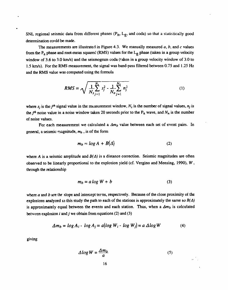
The Z$?Zbvalues for different eveilt pairs are listed in Table 4.1 and shown in Figure 4.4 for

each station. From Figure 4.4 it can be seen that t!~eZ@ value is less than 1 for Mission Cyber /

Disko Elm and Mission Cyber / Distant Zenith. From regional seismic data collected at the LLNL

stations, the value of the slope, a, in equation (3) is observed to be approximately 0.9 for the Pn

phase (Vergino and Mensing, 1990) and 0.8 for the Lg phase (Patton, 1988). Using an average

value of 0.85 for the slope, we have listed the values for.the cwrected magnitudes. From equation

(5), these values suggest that Mission Qber is a factor of 0.75 that of Disko Elm and 0.65 that of

Distant Zenith, and that Distant Zenith is a factor of 1.22 that of Disko Elm. To estimate the relative

seismic coupling between the three events, it would be necessary to calculate the percentage

difference between the yield ratio estimated from equation (5) and the actual ratio. Performing this

calculation suggests that either Disko Elm coupled high and/or both Mission Cyber and Distant

Zenith coupled low.

TABLE 4.1

hnb VALUES FOR NUCLEAR EXPLOSIONS USED IN THIS STUDY

RATIO &b o N bb / 0.85

MISSIONCYBER / DISKO ELM -0.106 0.081 36 -0.124

DISTANT ZENITH / DISKO ELM 0.073 0.068 30 0.086

MISSION CYBER / DISTANT ZENITH -0.161 0.112 20 -0.189

5.0 Conclusions

Data from the three tests conducted in P Tunnel have been analyzed from a number of

different standpoints in an effort to determine if any basic differences exist with regard to the

response of the tuff to the nuclear detonations. We have examined the quality of the rock, the

response of close in stress and accelerometer gages, and the response of far field seismometers. We

have compared the results from the P Tunnel tests with results from tests conducted in other tunnel

testing.

Our examination of the core in P Tunnel indicated that the quality of rock at all three

locations was strong and competent, at least out to a radius of 60 m from the working point, In fact,

we believe the strength of the tuff in the vicinity of Mission Cyber working point was better than

1‘7

.

would be indicated from looking at the resdts of static testing conducted by Terra Tek. In general,

the core located away from the working points in a vertical direction was found to contain many

layers cf very weak, sandy-like material, some layerc a few centimeters thick and some many

meters thick. This Iayering characteristic should be incorporated in the constituent model for more

accurate predictions of the ground niotion at close-in as well as seismic distances. Even though

these weak areas are well removed from the working point, they are still located close enough so

that reflections could affect the outgoing pulse shapes. It is also felt that future testing should

attempt to determine characteristics of this very weak unconsolidated material and its behavior under

dynamic loading. The current rational for determining properties for use in the various predictive

codes do not incorporate effects of these weaker layer,’ because test samples cannot be fabricated

due to the inhenmt weakness of the material.

Differences were found in the mineralogic content and the level of saturation of the tuff for

the Mission Cyber test (compared to the other two test sites) and these differences could account for

some of the scatter observed in the ground motion measurement records but would not result in

great difference in behavior.

With regards to our examination of the close in stress and accelerometer gages there are

several results that are puzzling. The arrival times of the peaks of the stress pulses from at least

four, and as many as seven, of the stress gagus from the Distant Zenith event could be interpreted as

having late arrival times compared to the other Distant Zenith stress gages and stress gages from the

other two tests. We could not correlate the identity of these gages with those that Sandia indicated

could have been affected by the presence of known faults. The four gages with the largest delay

were not singled out by Sandia as being of any signitlcant problem. Of the other three stress gages

which showed a smaller apparent time delay only two were identified by Sandia as 5eing directly

behind a known fault. O:iler gages that were identified by Sandia as being behind the fault actually

had earlier times of arrival of peak stresses rather than later ones. In addition, Sandia had also

identified accelerometers which were located behind a fault, but we found no abnormalities in the

times of arrival (either peat arrival times or arrival times of fwst signal) in any of the accelerometers.

It was also puzzling that the same stress gages that exhibited the late arrival time of the peak stress

showed no abnormality in the arrival times of the first signal. Sandia indicated that the faults caused

significantly reduced peak stress values. For some of the accelerometers records believed to be

influenced by the fault, the peak values were four to five times higher than expected, The fact that

faults would cause a decrease in the recorded stress values but an increase in the accelerations (and

velocities and displacements) seems unconvincing. In the end, the argument that the presence of

faults greatly alter the data from Distant Zenith was discarded and the variations ‘.vereattributed to

datz scatter.

An examiriation of the magnitudes of stress, acceleration, veloclty, and displacement,

18

indicated that of the three tests there was less scatter in the Disko Hrn data. The measurements from

I?isko Elm compare best with results obtained from testing in other tunnels. The most scatter

appears in the data from Distant Zenith and the scatter is to both sides of the fit to the Disko Elm

data. That is, some of the results from Distant Zenith are significantly higher than would be

expectec? and some are significantly lower. “ihere was very little scatter in the data from Mission

Cyber and all ot the data fall on the lower edge of the scatter from the Distant Zenith test. In

gener~, the behavior of the tuff as determined from the average of all three P Tunnel tests is below

the response determined m other tunnel testing.

Our examination of the rise times and pulse widths of the acceleration and stress records

indicates that the behavior of Distant Zenith is in general different from the results of Mission Cyber

and Disko Elm. Both the pulse widths and the rise times of the accelerometer records from Distant

Zenith are significantly larger than from the othe; two cvetits - but the rise times of the stress pulses

from the Distant Zenith event are in agreement with similar rise times from the other two tests. This

result appears to be contrary to our findings or. apparent delay of arrival of peak values of the stress

peaks. If the rise times are larger for the acceleration i)eaks thart expected the arrival times of these

peaks would be later, but they were tiot. If the rise times of the stress peaks was normal then it

would b! expected that the arrival times of those peaks would be normal, but they were Iatcr than

expected.

There was good agreement ayong the rebound times among the three P Tunnel tests - both

for the start of rebound and the end of rebound. Our examination did indicate that the total amount

of time that movement back towards the source occurs appears to ‘beconsiderably less (about 50%)

for the P Tunnel tests than for Hunter’s Trophy - an N Tunnel event. This should be investigated

by examining the amount of displacement back towards the source in the P Tunnel tests compared to

other tunnel testin~ ~maller elastic rebound could help explain anomalies in the differences

between dynamic and ‘ ~. ianent displacements that occurred, especially in the Mission Cyber

event.

From the standpoint of the shape of the stress pulse the “impulse” as determined fiorn an

integration of the stress versus time record appears to be greater for the Distant Zenith event than for

the other two tests. Bear in mind that the results from such an integration should be viewed with

some speculation since the stress does not return to zero because of residual stresses which made it

necessary to select somevifat arbitrarily the up~.r limit on the time of integration.

The results of the seismic analysis indicated that Mission Cyber looks small compared to

Disko Elm but also indicates that Distant Zenith looks smaller than it should compared to Disko

Elm.

Our detailed analysis of the results from the P Tunnel tests has. therefore, lead us to the

conclusion that there is no real reason to believe that the results obtained from the Mission Cyber

19

test are vastly different from the results obtained from the other two P Tunnel tests, The results

from Mission Cyber fall within the scatter band which was determined from Distant Zenith and

Disko Elm. Unlike Distant Zenith, all of the Mission Cyber points simply fall at the lower edge of

the scatter band. Of the three tests Distant Zenith appeared to have the most scatter and Disko Elm

the least.

Acknowledgments

Many people have contributed to our study. We acknowledge Carl Smith and Bob Bass at

the Sandia National Laboratories for providing the ground motion and stress records from Mission

Cyber, Disko Elm, and Distant Zenith and for taking time to discuss these shots with us. We thank

Barbara Harris-West at the Defense Nuclear Agency at the Nevada Test Site for her assistance in

arranging for us to examine the core, fo- collecting ground motion data for us, and helping us

understand the tuff properties in P-Tunnel. The cooperation and expertise of Byron Ristvet at the

Defense iquclear Agency in Las Vegas, NV is very much appreciated. We appreciate Fred App’s

contribution in helping us interpret ground motion data from the tunnel tests. We appreciate the

assistance of Jerry Magner, Mark Tsatsa, Ron Martin, Dick Hurlburt, and Harry Covington at the

United States Geological Survey core library at the Nevada Test Site. We thank Susan Freeman for

shcwing two of us (WLF and RDD) around Rainier and Pahute Mesas at the Nevada Test Site. We

thank Doug Seastrand for providing SNL seismic data and Amanda Goldner and Keith Nakanishi

for providing LLNL seismic data. We thank Eric Jones for reviewing the report. This work is

performed under the auspices of the U.S. Department of Energy by Los Alamos National

Laboratory under contract W-7405-ENG-36.

20

●

References

Bass, R.C., “Free-Field Ground Motion Induced by Underground Explosions”, Sandia Nationallabomtory Report SAND74-0252, 1975.

Brady, L.F., “The Sandia Seismic Network,” Sandia National Laboratory, Albuquerque, NM,EGG 10617, llpp, 1989.

“Containment review of the DNA Mission Cyber Event (U),” Presented by DNA forpresentation to the 166th CEP Meeting, 1987.

“Containment review of the DNA Disko Elm (U),” Presented by DNA for presentation to the179th CEP Meeting, 1989.

“Containment review of the DNA Distant Zenith Event (U),” Presented by DNA forpresentation to “he CEP Meeting, 1991.

Foumey, W.L., R.D. Dick, and T.A. Weaver, “Explosive shielding by weak layers,”l%xxeding~ of the Numerical Modeling for Underground Nuclear Test MonitoringSymposium, Durango, CO, March 23-25, 1993, S.R. Taylor and J.R. Kamm, Eds., LosAlarnos National Laboratory Report LA-UR-93-3839.

Jarpe, S.P., “Guide for using data from the LNN seismic monitoring network,” LawrenceLivermom National Laboratory, Liverrnore, CA, UCID-21872, 5pp, 1989.

Patton, H.J., “Application of Nuttli’s method to estimate yield of Nevada Test Site explosionsrecorded on Lawrence Livermore National Laboratory’s Digital Seismic System,” Bull.Seis. See. Am. ~, 1759-1772, 1988.

Torres, G. “Characterization of material from the Nevada Test Site, final report for the periodJanuary 1986 thrcugh March 1988 - Volumes 1,11, III,” DNA-TR-88-278-V1, V2,V3,1988.

Vergino, E.S. and R.W. Mensing, “Yield estimation using regional mb(pn),” Bull. Seis. Sot.Am., ~, 656-674, 1990.

21

FIGURE CAPTIONS

Figure 1.1 Tunnel Level Map of Mission Cyber (U 12P.02), Disko Elm (U 12P.03), and DistantZenith (U 12P.04) and the Location of the Exploratory Core Holes.

Figure 12 Stratigraphic Section and the Event Level at Which the Three Tests Wem Conducted.

Figure 1.3 Disko Elm Exploratory Horizontal Holes and SNL Instrument Holes Typical for TheseTest Locations.

Figure 2.1 Relative Strength Versus Depth for the Vertical Core Hole UE12P.04 Near MissionCyber.

Figure 2.2 Relative Strength Versus Depth for the Vertical Core Hole UE12P.04 Calibrated fromTerra Tek Strength Data.

Figure 2.3 Relative Strength Versus Length for U12P II-I-l.

Figure 2.4 Relative Strength Versus Length for U12P.06 UG-1.

Figure 3. la Typical Stress Measurements From Mission Cyber Event.

Figure 3.1b Typical Stress Measurements From Disko Elm Event.

Figure 3.1c Typical Stress Measurements Fmm Distant Zenith Event.

Figure 3.2a Typical kceleration Meamuements From Mission Cyber Event.

Figure 3.2b Typical Acceleration Measurements From Disko Elm Event.

Figure 3.2c Typical Aeeeleration Measurements From Distant ZeNth Event.

Figure 3.3 Time of Arrival Versus Scaled Range for Peak Stress Values From DZ Compared toLeast Square Fit of DE and MC Data.

Figure 3.4 Stress Measurements From Three P Tunnel Events Compared to Expected Results. 1-Distant Zenith, 2- Mission Cyber, 3- Disko Elm.

Figure 3.5 Acceleration Levels Measured in P Tunnel Events Compared to Expected Results 1-Distant Zenith, 2- Mission Cyber, 3- Disko Elm.

Figure 3.6 Vehxities Measured in P Tunnel Events Compared to Expected Results. 1- DistantZenith, 2- Mission Cyber, 3- Disko Elm.

Figure 3.7 Dynamic Peak Displacements From DE and MC Compared to Permanent DisplacementsFrom MC.

Figure 3.8 Acceleration Pulse Width Comparison of Results From Three P Tunnel Events - Linesare Least Square Fits. 1- Distant Zenith, 2- Mission Cyber, 3- Disko Elm.

Figure 3.9 Acceleration Risetime Comparison of Results From Three P Tunnel Events. 1- DistantZenith, 2- Mission Cyber, 3- Disko Elm.

Figure 3.10 Typical Velocity Trace Showing Two Rebound Times - RB 1 and RB2. .,22

Figure 3.1 la Rebound Time RB 1 From Three P Tunne! Events and From Hunter’s Trophy.

Figure 3.11b Time llmtion of Velocity Towards Source (RB2-RR 1) Frum Three P Tunnel Eventsand For Hunter’s Yrophy.

Figure 3.12 Comparison of “Impulse” (Area Under Stress Time Curve) From Three P TunnelTests - Lines are Least Square Fhs. ! - Distant Zenith, 2- .MissionCyber, 3- Disko Elm.

Figure 3.13 Frequency Spectra From Two Accelerometers From Dis(ant Zenith Showing LargeDifference in Rol! Off.

Figure 4.1. Location of seismic stations of the Liverrnore NTS Network (LNN; open triangles) andthe Sandia Seismic Netwo* (open circles).

Figure 4.2. Vertical-component seismograms at LLNL station KNB (Kanab, U“~)for Disko Elm(solid line) and IWssion Cyber (dashed line) on the high-frequency channel and the broad-bandchannel (high-pass filtered at 0.5 Hz).

Figure 4.3. Examples of measurements on the hi@-frequency vertical-component seismogram atKNB. Top portion of the figure shows measttmmems used to calculate a, b, ard c values fromthe Pn wave ( a = T1 -O; b = I T1 - T2 1;c = IT3 - T21). The bottom portion of~he figure showsthe windows used for the Lg RMS (T4 to T5) and coda RMS (T5 to T6) calculations (band-passfiltered between 0.75 and 1.25 Hz).

Figure 4.4. Anb values and 20 errors for different measurements and event pairs. (a) MissionCyber / Disko Elm, (b) Distant Zenith / Disko Elm; and (c) Mission Cyber / Distant Zenith.Station indicators (see Figure S1): B - BTM; D - DRW; L - LDS; N - NLS; T - TON; EH - ELKHF; KH-KNBHF; LH-LACHF; MH-NINVHF; EB-ELKBB; KB-KNBBB; LB-LACBB; MB - W BB.

23

. .-

9,

lE12PolE12Pm Q

,.

l?@ure 1.1

mm mmALTITUE ALTIU

[feet) (mmrs)

6400

F

Tu. . .. . .... .. ..’..

..” ,.. . T-.. -.:’... . . . .“. “.:;..”,

. “.”:..;”.::.; ,:..,

6ooo- !“. . ~.’.””

.mT@w.. . . . .. . :... .*

.

S60075Htt

Tp-

9

-

Tt4-

4400

-2100

-2000

“ 1=0

“ lmo

■

m

m

1600

190

1400

.

1

ORILL HOLE DESCRIPTION

\

—

T8MM?OMMTCMU?6NMrowTWlurowT9MM7oun7QMU7WM70-

a;::

t 8MM78MN

?SwT6MMmmn70UM79NHMMU

fs.m10U

1.8M1.8M1.OM1.SU1.ON1 .Ou*M1,s9“m1.8n

Tiullra 1.’3

.

.

lo-

9-

8-

7-

6-

5-

4“

3.

2.

1.

0“

UE12P#4VERTICAL CORE MISSION CYBER

E-E3a=i=-.. ...... . .. .

...........”-.-

0306191 la 152 1DEPTH (M)

1........... ..........fl------ ..-...-..–..‘...-

~1

+

I1 }-...-–—.~-.—---..-.-..—-...l”..- ....— -.-,

Figure 2.1

UE12P#4VERTICAL CORE MISSION CYBER

“9 —“”””---”””----”’-~■ ■

8 d - .....—. —.-+ * ~+-””

7 -—--..-.”.,.—.....—.—.--.-.-——I ++

. m .

0+ I 1 I I -1 I

0 m Iw Im 3DEPTH (m)

+Authwa

FiEuro 2 ● 2

.

10

9

8

7

6

5

4

3

2

1

0

U12P.02 IH-IINSTRUMENT HOLE MISSION CYBER

...--- .."- .-------- .-. -.- . . . . . ..- . .. - .-- __.. __-. --. ". "."..-.. . . . . . . . . —.-- . . . . . . . . . . . . . . . . . . . . . . . . . . . . . . . .

0 1s 30 48 61 76 91 107 122 137DEPTH (M)

.t . .

Figure 2.3

.

.

-—

U12P.06 UG-IHORIZONTAL CORE P-TUNNEL

f-------’-r-”-”-””--4+—

Figure 2.4

2

1.6

1

0.6

0

-0.6

-1

Typical Stress MeasurementsJfimioat Cyhr Bvont

!0

I

●

✎

o

Typical Stress MeasurementsDisko Elm Event

I 1 i I

10 20 30 40 50 60Time (Scaled Mi.llitmconclfi)

Figure 3.lb

●

●

Typical Stress MeasurementsDistant Zenith Event

3

2

1

ao 20 io 60 00 100 120 140 160

Figure 3.lc

.

2500

2000

1500

1000

500

0

-500

Typical Accelerometer MeasurementsMission Cyber Event

.............. ..................

......................................

........................

.............

..............

..............

h.. ....................................................................................................................................... .

II I

50 100 ~ 150 2Time (Scaled Mi,llisecomls)

Figure 3.2a

.

Typical Acceleration MeasurementsDisko Elm Event

4000

2000

.

0

-2000o 10 20 30 40 50 60

Time (Scaled Milliseconds)

Figure 3.2bI

.

.

3500

3000

2500

2000

1500

1000

500

0

-500-,

Typical Accelerometer MeasurementsDistant Zenith Event

8.......................................~

!

......................;.

...................

I

------+

...........................

i

I+......................

\].........................

..........................................n

Time (Scaled Milliseconds)

●

ii!i=

80

70

50

40

30

20

10

Distant Zenith EventStress Data

.I I i I I I r—l———l

20 40 60 80 100 120 140 160 180Range (Scaled Meters)

Figure 3.3

.

Pressure versus RangeTests of Interest

2

1.5- "-""--"--"""-""---"-""--"-"-"-----"----------"----"""-" .......................................

1- -“””-–----.----”-.-””---”-””-..”-”- \o.5- -“-–”--”--””------””-----”””--””------”

o- -“----”---”--.-..—..-. ..--..............................................................................

-o.5- ..............................................................

-’1- ............................................................

–o 0;5Log

i 1;5 2 2.5

Range (m)

—— +1 SD DZ & DE Dat ----= -1 SD DZ & DE Data — Mean of All Data

Figure 3.4

.

.

4

3.5

3

2.5

2

1.5

1

0.5

Acceleration versus RangeTests of Interest

,.....-.. --.. —..-. .. ...

..... . .... .... .... .. ....... . ......... .. .......

. . . . .... ..... .. .. . ....................... ... ......................... ..... .

........................................................................................................ ............ . ............................................................

0:.

I 1 I I I

1.2 1.4 1.6 1.8 2 2.2 2.4Log Scaled Range (m)

— +1 SD for DZ & DE ==-- -1 SD for DZ & DE — Mean of All Data

... ,

Figure 3.5

.

●

2.5

2

1.5

1

0.5

0

“0.5

-!

Velocity vs Scaled RangeTests of Interest

~-................._*..w___ .. ........................

................ .. ....... ................................................................~..

=“’-””””-:~---------------------------------...............................................................................................................

‘~h~--------------------.--.1--------------------

.....................................................................................................................................................- 3>..-.--->$---37----{

I 1 I I I I 1 I I

4

{

1.5 1.6 1.7 1.8 1.9 2 2.1 2.2 2.3 2.4Log Scaled Range (m)

— +1 SD DZ & DE ●-=-====-1 SD DZ & DE — Mean All Data

Figure 3.6

Displacement Comparison

I=””:””””::F i ~ ~ ~ ~ - ~~

x ...............m....................................................................

10 100 ‘ 10Range (scaled meters)

00

= MC - Peak * MC-Permanent ❑ DE - Peak

Figure 3.7

.

●

1.2-

1-

0.8-

0.6-

0.4-

cl.2-

0

-0.2

-0.4

-0.6 10.

P Tunnel TestsAccelerations Scaled Values

'--=---:z:~~~R5"........................I.Q.......

v"--"""""""""""----""""""""""1 1 1 I I

1 1 1.2 1.4 1.6 1.8Log Time of Arrival (milliseconds)

-u- Mission -t- Disko ~ Distant

Figure 3.8

P Tunnel TestsScaled Values/Accelerations

1.2

1- """"""""""""""""""""--"""-""""""--""""-""-""""""""""""""""'"""""""""-'"""""""-""""""""-"-"""-"'"""""""""""""""""""""""""""""""""""""""""""--""-""'-"----'"-"1,

0.8- --"""""-"""'"`"""""""-""""""""""""-"""""---'"""-""'-""`-""""""""""""""""-"""""""""""""""-"""--"-q“””””””””””””-”””’’”””””””””’”””o.6- ................................. p~ ~........................................................ .... .. ............. ....... .................... .......................... ..................................

0.4- “-”---””-”----”--””-”’” ‘--- ■ ‘w ‘g-a-””g-”’”””””

1

0.2 “’””””””-””---”---”

~~2:::::::o ““””’”””””’””””””””“’”3”””7’3-””

i c/------0.2 ................ . . ... . ... ...!?..... ...-..oo44..............Z ....................g...............................................................................................................................................................

-0.6 [ 1 I0.6 0.8 1

Log Time of Arrival1:2

~..

1:4 1.6 1:8

(milliseconds)

■ Mission --+ Disko +++-- DistantL

5

4

3

2

1

0

-1

-2

Typical Velocity Curve

........................................................................................................................................................................................................................................

................................................. ......................................................................................................................................................................................

..................................................................................................

............. ..................................................................................................

....................................................................................

................................................................... ........................

I I I I I

100 200 300 400 500 6Time (Scaled Milliseconds)

Rebound 1 Time Versus RangeTunnel Tests

.............................................................................. ................... ...............................................................................

10 I I I I 1 I I I I I A

10 100 ~ 1000Scaled Range

ru ‘Mission + Disko * Distant ❑ Hunter’s

FiQure 3. lla

rime Duration of Velocity Toward SourceTunnel Tests

1000

l!!i=

10

.............................................................................E ......R..Q.......Q............................................................•1

- –~~ I I I I I I I I

J 100 1000Scaled Range

= Mission + Disko * Distant ❑ Hunter’s

Figure 3.1 lb

.

1.5

1

0.5

0

-0.5

-1

1

“impulse” versus RangeP Tunnel Tests

K.....-.*.- 7

"-"-"-"m+::"""""""""`""""""""""'"""'""'""'"""""""""""'"""""'"'"""""m""""'"...................................................................

............g2.n.a-~“”””””’””?”””””””-:;-:”

.............................

■? ●

---..=~ ‘%---.....7

......................................................................................................?. 7=u:::: ...............u.3. ....................................o.........................---

-’”--~z

1 I 1 I I I I

3 1.4 1.5 1.6 1.7 1.8 1.9 2

— LSF DE --------LSF MC =0”0=00LSF DZ.—

1

Log Range (scaled meters)

Figure 3, 12

Frequency Spectra - Distant ZenithTwo Accelerometers

0.1 "t,,,, t:,,,,,"J,,t,,8,,,::,,,,,",,,,,,,,tt,,,U",,",,,,2,,,,,,,,iUt,#,,,,,,t,,,,U,,Z,,,,S>,,,,,,,,,t,,,,,,tt,,t,,,i,",,,,,:,t,`,,`,,,,,,,,,,,,",it,,,,,,U,,,,,,,,,t,,,,",,,,,,,,,,,,,X`,:,l:,,:,,,,,,,,,:,:,. . . . . . . . . . . . . . . . . . . . . . . . . . . . . . . . . . . . . . . . . . . . . . . . . . . . . . . . . . . . . . . . . . . . . . . . . . . . . . . . . . . . . . . . . . . . . . . . . . . . . . . . . . . . . . . . . . . . . . . . ......................................................................... ............ . . . . . . . . . . . . . . . . . . . . . . . . . . . . . . . . . . . . . . . . . . . . . . . . . . . . . . . . . . . . . . . . . . . . . . . . . . . . . . . . . . . . . . . . . . . . . . . . . . . . . . . . . . . . . . . . . . . . . . . .................................................................................... . . . . . . . . . . . . . . . . . . . . . . . . . . . . . . . . . . . . . . . . . . . . . . . . . . . . . . . . . . . . . . . . . . . . . . . . . . . . . . . . . . . . . . . . . . . . . . . . . . . . . . . . . . . . . . . . . . . . . . . ....................................".......................................................

. . . . . . . . . . . . . . . . . . . . . . . . . . . . . . . . . . . . . . . . . . . . . . . . . . . . . . . . . . . . . . . . . . . . . . . . . . . . . . . . . . . . . . . . . . . . . . . . . . . . . . . . . . . . . . . . . . . . . . . . ....................... . . . . . . . . . . . . . . . . . . . . . . . . . . . . . . . . . . . . . . . . . . . .

0.01 :::z::::::::::::::::::::::::::::::::::::::::::::::::::::::::::::::::::::::::::::::::::::::::::::::::::::::;::::::::.:::::::::::::::::::::::.:,lul:at,*ll,`*,,, t,$,,*,,,,,!,*, *,,,:,,,,,,,,,, t*, t,*,,,,,`,,,*,,it,,,,,i *,*::,,:: tt::t,,,,,,.l, t,,t,t`,,,,,*,,,,:, z,:4`,, *:,,$,,:,:,,,, i`,,,,,

. . . . . . . . . . . . . . . . . . . . . . . . . . . . . . . . . . . . . . . . . . . .. . . . . . . . . . . . . . . . . . . . . . . . . . . . . . . . . . . . . . . . . . . .

. . . . . . . . . . . . . . . . . . . . . . . . . . . . . . . . . . . . . . . . . . . . . . . . . . . . . . . . . . . . . . . . . . . . . . . . . . . . . . . . . . . . . . . . . . . . . . . . . . . . . . . . . . . . . . . . . . . . . . . . ......................?18:11:1;,,1,,,:,,,,,,,,:,:,:,:,,,:,:,,,:,,,

. . . . . . . . . . . . . . . . . . . . . . . . . . . . . . . . . . . . . . . . . . . . . . . . . . . . . . . . . . . . . . . . . . . . . . . . . . . . . . . . . . . . . . . . . . . . . . . . . . . . . . . . . . . . . . . . . . . . . . . . ......................... . . . . . . . . . . . . . . . . . . . . . . . . . . . . . . . . . . . . . . . . . . .

. . . . . . . . . . . . . . . . . . . . . . . . . . . . . . . . . . . . . . . . . . . . . . . . . . . . . . . . . . . . . . . . . . . . . . . . . . . . . . . . . . . . . . . . . . . . . . . . . . . . . . . . . . . . . . . . . . . . . . . . ...................................................................................... . . . . . . . . . . . . . . . . . . . . . . . . . . . . . . . . . . . . . . . . . . . .

. . . . . . . . . . . . . . . . . . . . . . . . . . . . . . . . . . . . . . . . . . . . . . . . . . . . . . . . . . . . . . . . . . . . . . . . . . . . . . . . . . . . . . . . . . . . . . . . . . . . . . . . . . . . . . . . . . . . . . . . . ..............................................................................

:!::n!x!:wamn!: %!!u., .-...w..."..", . . ..".* . . . . ..o . . . . . . . ..oo.o* . . . . . . . . . . . ...*.."".

. . . . . . . . . . . . . . . . . . . . . . . . . . . . . . . . . . . . . . . . . . . . . . . . . . . . . . . . . . . . . . . . . . . . . . . . . . . . . . . . . . . . . . . . . . . . . . . . . . . . . . . . . . . . . . . . . . . . . . . . . . . . . . . . . . . . . . . . . . . . . . . . . . . . . . . . . . . . . . .................. ...........................

1

1

1

1

E-06i................"......."......................".".........."..........................................- --{116 m w--’-W

::w!fiwifimx!I:-:{iHfiHHxi?::?ww!*!::ifi!w:!iIi+fi::R3::ii.wi,w,%%dfi::::!:::!!!':fi!lti*:ll:ltl:`**:*i*t,ii,t*,lll:,tt,**,,t,*t,,*t,,,,,t,,,,,,**,,,,,,t*,,,*,,,,,,~,,,,*,,,,,,*,,ti,,,i,,,*,tt,,,,,,,t,,,,,,,,,,,,,,,,,,,,,,,,*t,,>,,*,,,,,,,,,,,,,,:,:...............................................................................................................................................................................................................................................................................................................................................................................................................................................

E-074 llllllllllllIflllllllllllllIlllllIII!jlllIllllllIIIl!illllII!lllIillIIIl!lllllI!lllllllllllllilIlllllIll!lllllllllI!lllllll}l!llllIlllilIlllI!l{illllllllllElllllilllliillllIlll}llU!Iilll!lIIIIlllliIi!lil!!liiIl!i!!:::X%: :X:X :M::ww: ::.:;.:fi::::::%:::::: ::::U:::::::: ::.:.:::::::::.::::::::::::::::.::::.:::::::::::Y.xfififi:.: ::XX::W; :.::::::::.::::::::::::::::p.::::::::::::...............................................................................................................................................................................................................................................................................................................................................................................................................................................I4E-08 ::t:iti:~t!!~tijt,:,iIififii~fiifiiiiifiii;iififi~fifi;fiiiiiiifi~i~i~fiii~iififi;iiiiiMiiifiitiiiliiifititifiiNfiiiiiWt;liW!:ifi~MilfiiWiiifiiiliiiiiiiiiiiiiiiii

.... . . ............

::::*{:::::::::W.::::2::% ~.:H::::::::::::::L::tX:%:~:X ::::::::f:::U.:V.::::::t:t:fl.ti::~::::::~~::fl ::WN:WW.: :U.:Y.::X:: ?.?.W:: H::::::::7.:::::::::::::2::::::::::!::::::::::::...... ..........................................................................................................................................!..........................,........................................................................................................................................................................................................ .....................................................................................................................................................................................................................,...........!,.........................................I

E-09 ! 1 I I I 1 I ---1---1

100 1000Frequency (Hz)

Figure 3.13

I 1

A LAC

}

.

Figure 4.1