Losing Heart? The Effect of Job Displacement on Health

1

Losing Heart? The Effect of Job Displacement on Health

by

Sandra E. Black Department of Economics

University of Texas, Austin, IZA and NBER

[email protected]

Paul J. Devereux School of Economics and Geary Institute

UCD, CEPR and IZA [email protected]

Kjell G. Salvanes

Department of Economics Norwegian School of Economics, IZA, and CEE

[email protected]

October 2012

Abstract Job reallocation is considered to be a key characteristic of well-functioning labor markets, as more productive firms grow and less productive ones contract or close. However, despite its potential benefits for the economy, there are significant costs that are borne by displaced workers. We study how job displacement in Norway affects cardiovascular health using a sample of men and women who are predominantly aged in their early forties. To do so we merge survey data on health and health behaviors with register data on person and firm characteristics. We track the health of displaced and non-displaced workers from 5 years before to 7 years after displacement. We find that job displacement has a negative effect on the health of both men and women. Importantly, much of this effect is driven by an increase in smoking behavior. These results are robust to a variety of specification checks. * We thank participants of seminars at Uppsala University, Norwegian School of Economics, IZA, Royal Holloway, and the Bergen-Stavanger Workshop for their helpful comments. The authors thank the Norwegian research council for financial support, and Devereux thanks the Irish Research Council for the Humanities and Social Sciences (IRCHSS) for financial support. We thank the Norwegian National Health Institute for providing us with the health data, and, in particular, Kjersti Andersen Nerhus, Inger Cappelen, and Sidsel Graff-Iversen for very helpful discussions about interpreting the data.

2

1. Introduction Job reallocation is considered to be a key characteristic of well-functioning labor markets, as

more productive firms grow and less productive ones contract or close. However, despite its

potential benefits for the economy, there are significant costs that are borne by displaced

workers. While a large literature focuses on income losses from displacement, much less is

known about the health impacts of these types of job loss. This issue is particularly salient

given the large increases in unemployment that have occurred over the last few years during

the economic downturns.

There are several mechanisms through which job displacement may affect health. Job

displacement increases stress, which is known to have negative effects on cardiovascular

health. However, there is little evidence on the link between specific causes of stress, such as

changes in employment status or earnings losses, and cardiovascular health. 1 Changes in

income induced by displacement could also affect consumption patterns, which could have

either a positive or negative effect on health. For example, a person may respond to the

reduction in income by reducing consumption of cigarettes and alcohol or, in contrast, by

reducing consumption of fresh fruit and vegetables. Finally, changes in employment status

that accompany displacement may affect time spent on exercise and, in this way, impact

health.

In this paper, we examine how job displacement in Norway affects cardiovascular

health directly using a sample of men and women who are predominantly in their early

forties. Our unique dataset merges registry data on the population of Norway with newly

available representative survey data on health and health behaviors. Using plant identifiers,

we determine which employees lose their jobs due to plant closings or mass layoffs and track

the health of displaced and non-displaced workers from 5 years before to 7 years after

1 See Bosma, Siegrist and Marmot (1998) and Kirvimaki et al. (2002) for evidence.

3

displacement. We focus on the effect of displacement on heart-related variables (cholesterol,

blood pressure, smoking, body mass index) as well as on two indices that measure the risk of

heart disease. Our focus on heart-related variables relates both to the data available to us but

also to the importance of heart-related conditions -- cardiovascular disease (CVD) is a

growing problem throughout the world; in the United States alone, more people die from

CVD than from cancer, and heart disease is a major risk for people aged 40 and above.

Our work has a number of advantages over existing work. We observe the population

of Norway, so we are able to follow a large number of displaced workers including those

leaving the labor force. In addition, our health survey data contains diagnostic tests,

including blood pressure and cholesterol, along with information about specific health-related

behaviors such as smoking.

We find that job displacement has a negative effect on health of displaced workers.

Importantly, it appears that much of this effect is driven by increases in smoking behavior for

both men and women. Interestingly, there is no equivalent health effect on the spouses of

these workers. However, we do find some negative health effects on workers in downsizing

firms even if they themselves are not displaced. These results are robust to a variety of

control groups and specification tests.

The paper unfolds as follows. Section 2 presents the literature review, Section 3

describes the institutional features of Norway during this time period, and Section 4 discusses

our empirical strategy. Section 5 describes the data and Section 6 presents results and a

variety of robustness and specification checks. Section 7 concludes.

2. Related Literature

There is a large literature on the effects of job displacement on earnings. While the

consensus is that earnings decline significantly post-displacement, the magnitude varies

4

considerably across countries. Researchers have found huge earnings losses for displaced

workers in one state in the U.S. in the 1980s, up to 25% soon after displacement (Jacobson,

LaLonde, Sullivan, 1993), and these results have been confirmed more recently by

representative data for the US (Hildreth, von Wachter, and Weber Handwerker, 2012).

Earnings losses in Europe have generally been found to be much smaller (from 1-15 percent)

but there are often large effects on time out of employment. (See for instance Eliason and

Storrie, 2004; Burda and Mertens, 2001; Carneiro and Portugal, 2006; von Wachter and

Bender, 2006). In Norway, previous research has found earnings losses from job

displacement of only about 5% (Huttunen, Møen, Salvanes, 2011).2

There are also a number of papers on the relationship between general labor market

conditions and health. For example, Ruhm (2000, 2005) shows that recessions are generally

good for health; economic downturns reduce mortality and economic expansions are

associated with negative health effects, despite the protective effect of income. Recent work

by Asgeirsdottir et al. (2012) uses data from the 2008 economic crisis in Iceland to examine

the effect of a macroeconomic shock on health and health behaviors. Overall, their

conclusions were ambiguous; they find that the economic crisis was associated with

reductions in harmful behaviors such as smoking and heavy drinking. This was combined

with a reduction in the consumption of fruits and vegetables and an increase in the

consumption of fish oil and improved sleep behavior. While these papers examine the

overall health consequences of macroeconomic shocks, we focus on the effects of a specific

economic shock to an individual, controlling for general macroeconomic conditions.

2 There is also a relatively small but growing literature on the effect of job displacement on other outcomes. Rege et al (2009) show that job displacement is associated with increased criminal behavior. Page, Oreopoulos and Stevens (2008) find that children of fathers who were displaced earned 9% less than children of fathers who did not experience a job displacement. Rege, Telle, and Votruba (2011) use data from Norway and find that father’s displacement has a negative effect on children’s academic performance, while mother’s displacement has a positive effect.

5

There is a much smaller literature focusing on the relationship between job displacement

and health outcomes. At the extreme, recent studies have examined how job displacement

affects mortality rates. Sullivan and von Wachter (2009) find higher mortality rates for

displaced workers in the U.S. in the 1980s (50-100% higher soon after displacement), with

evidence suggesting that these effects are due to the associated decline in income. Equivalent

increases in displacement have been found to lead to smaller increases in mortality in Sweden

and in Denmark (Eliason and Storrie, 2009b; Browning and Heinesen, 2012). Eliason and

Storrie (2009a) use Swedish register data and find that mortality risk among men increased

substantially during the first four years (44%) following job loss, with no effect on female

mortality. Browning and Heinesen (2012) use population data from Denmark and also show

that mortality increases significantly post-displacement.

However, mortality is a crude indicator of health status; other studies have attempted

to look directly at job displacement and health. Unfortunately, these studies have been

limited by either small datasets or indirect measures of health status. In the United States,

there are several studies of older workers using the Health and Retirement Survey (HRS).

Salm (2009) shows that health reasons are common causes of job termination; however, in

the case of exogenous job termination, he finds no evidence of effects on various measures of

physical and mental health. Because they are using the HRS, the study is limited to older

workers and, in the case of exogenous job loss, also faces relatively small sample sizes.

Strully (2009) examines the issue using health data from the Panel Study of Income

Dynamics (PSID) and finds negative effects of displacement for blue-collar workers but no

effects for white-collar workers; again, however, the authors are limited by small sample

6

sizes. The general finding in these papers is that displacement is bad for health, but because

they observe relatively few displaced workers, they are hampered by low precision.3

In contrast, recent European studies have used registry data with large numbers of

observations but have been limited by the absence of direct health measures. As a result, they

are forced to use more indirect measures of health status. Browning et al. (2006) use a 10%

sample of Danish register data to study stress-related hospitalizations and find no evidence of

an adverse effect of displacement. In more recent work, Browning and Heinesen (2012) use

data from the Danish population and find that displacement increases certain types of later

hospitalizations in Denmark. Rege et al. (2009b) use Norwegian register data to study the

effect of displacement on disability pension utilization and find displaced workers were 24%

more likely to have such a pension.

One notable exception is a recent paper by Bergemann, Gronqvist, and

Gudbjornsdottir (2011), which uses Swedish data to examine the effect of job displacement

on diabetes; they find that incidence of diabetes increases after displacement for single men

and for women with small children. Our paper has the advantage of the large sample sizes of

registry data combined with actual measures of health and health behaviors such as

cholesterol, blood pressure, and smoking.

3. Institutional Background

Employment Protection

Norway is considered to have a relatively high degree of employment protection

combined with generous unemployment benefits. When layoffs occur due to a downsizing,

there is no legal rule dictating which workers should be laid off. Seniority is a strong norm

and is institutionalized in agreements, but only where “all else is equal” is the firm supposed

3 Marcus (2012) uses German SOEP data to examine the relationship between job loss and health measures; unfortunately, he is also limited by small sample sizes.

7

to layoff a less senior worker rather than a more senior one. There is one important

exception: there are stringent restrictions that limit the capacity of firms to dismiss sick

workers.

Most employment contracts require 3 months notice of termination. There is no

generalized legal requirement for severance pay; however, workers may be induced to leave

voluntarily through severance pay and job search assistance.

Unemployment Insurance

Unemployment benefits are quite generous in Norway. The benefit is 62.4% of the

previous year’s pay, or 62.4% of the average over the last 3 years, and may be received for up

to 3 years. After this period, if still unemployed, a worker may be eligible for means-tested

social support. Unemployment benefits are included in our earnings measure, while social

support is not. About 78% of displaced men in our sample are re-employed one year after

displacement.

Disability Pension

Disability benefits are also quite generous in Norway. To receive a disability pension,

a person must be a resident in Norway for at least 3 years prior to disability. In order to

quality, it must be the case that “earnings capacity” is permanently reduced by at least 50%

because of illness, injury, or defect. Applicants require a doctor’s evaluation of health and

loss of earnings capacity. The pension equals some basic amount plus a function of previous

earnings. For low-income groups, the replacement rate is high and can be over one and, for

most people, it is over 0.5. As we will see later, disability pensions are not particularly

important for our sample.4

Overall, the generous social benefits in Norway are likely to help mitigate the

negative effects of displacement. As such, the estimated effects will likely underestimate 4 Rege et al. (2009) show that, in Norway, displaced workers are more likely to use disability pensions than other workers. However, this effect should be more relevant to older workers.

8

what the negative health effects of worker displacement would be in a less protective

environment.

4. Empirical Strategy

Our empirical strategy is a differences-in-differences approach that is motivated by

the data available to us. While our employment and earnings data are longitudinal, our health

data are cross-sectional in that we only have one observation per person.5 Therefore, we

cannot compare changes over time in health of individual displaced workers to changes over

the same period for the non-displaced. Instead, we compare changes in the conditional mean

of health for the displaced and non-displaced groups with the non-displaced operating as a

control group for the displaced.

A. Defining Treatment and Control Groups

The approach in this paper is to compare the post-displacement outcomes of displaced

workers to those of other workers who are not displaced. To operationalize this we need the

concept of a base year. One can think of the base year as the year in which the displacement

event did or did not occur. We follow people for 13 years in total – from 5 years before the

base year to 7 years after the base year. So for a given year in our sample, the treatment

group is those who were displaced in that year and the control group is those who were not

displaced in that year.

Complications arise because people can be displaced more than once in this 13-year

period and so, for example, their outcome in 1990 could be two years after a displacement in

1988 and two years before a subsequent displacement in 1992. To keep things tractable, we

(1) only consider the first displacement in the 13 year period for any individual and (2)

5 There are a few people who appear twice in the health data but not enough to enable us to undertake any longitudinal analysis.

9

exclude persons from the control group (the non-displaced) if they experience any

displacement in the 13-year period. This implies that we compare post-base year outcomes

for persons displaced at the base year but who experienced no prior displacement (in the 13-

year period) to persons who are not displaced in the same year and who experience no

displacement over the 13-year period. 6

Because we consider displacements that occur in several different years, in the

analysis we redefine each base year as year 0, with the year before displacement being year -

1 and the year after being year 1 etc. This enables us to run pooled regressions using all years.

In doing so, we always control for the year the displacement (or non-displacement) occurred.

We identify displaced workers using register files from 1986 to 1999. These files

include information on all Norwegian residents aged 16-74 in the relevant year. Importantly

for us, the files include both a person identifier and a plant identifier so we can identify

instances in which a person is working in a particular plant in a particular year but is no

longer with that plant the following year. Furthermore, we can identify plant closures from

situations in which a plant identifier disappears from the data and measure employment

changes at plants by simply counting how many workers are in each plant in each year. We

follow the previous literature by defining displaced workers as workers who separate from a

plant that closes down or reduces employment by 30% or more in the year that the separation

takes place. (See Jacobsen, Lalonde, and Sullivan, 1993). In addition, we treat workers who

leave a plant one year before that plant closes down (“early leavers”) as being displaced as

they are likely leaving because they are aware of the impending closure.

The data match workers and plants on May 31st from 1986 until 1995 and on

November 20th from 1996 onwards. For displaced workers, year 0 is defined so that they are

employed in May (November from 1996) in a certain firm in year 0 but no longer employed

6 Note that, because of these restrictions, an individual who experiences displacement will appear in only one base year while those in the control group could appear for multiple base years.

10

in that firm in May (November from 1996) of year 1 (and the period 0 firm has closed down

or downsized). This implies that there is uncertainty about the exact timing of displacement.7

Because of this, we consider years before the base year as being pre-displacement, years 0

and 1 as enveloping the displacement event, and years 2 to 7 as being post-displacement.

We restrict our sample to individuals with job tenure of at least one year who are

working full time (defined as working 30+ hours per week) when last seen at the plant before

the displacement event. Additionally, they must have positive earnings for the base year and

have had positive earnings in at least one of the previous 5 years (so we can calculate average

prior earnings). We exclude plants with fewer than 10 employees in the base year as it is

difficult to identify downsizings in very small firms. We use base years that run from 1986 to

1998.

B. Year-by-Year Regressions

To provide some initial evidence, we regress health in each time period on a dummy

variable for whether the person was displaced at time 0. That is, there are 13 separate

regressions going from t = -5 to t = 7. In each period the regression for health is as follows:

!!" = !! + !!!!! + !!!! + !

Here !!! is an indicator for whether person i was displaced at time 0, and !! is a vector of

other control variables. Note there is no t subscript on !! because the control variables are

time invariant. As described in more detail in the next section, our control variables include

base year dummies, survey dummies, survey month dummies, age at health measurement, a

dummy for whether the person is married in the base year, years of education at the base

year, birth order dummies, dummies for number of siblings, a dummy variable for whether

7 Base year 1987 – 1994: Displacement occurred between May of base year and May of the following year. Base year 1995: Displacement occurred between May of base year and November of the following year. Base year 1996 – 1998: Displacement occurred between November of base year and November of the following year.

11

the person was born in Norway, month of birth dummies, plant size in the base year (number

of employees), a quadratic in tenure in the base year, the average of the log real earnings

from t = -5 to t = -1, dummies for county of residence in the base year, 1-digit industry

dummies for the base year industry and, for men, IQ test score at age 18, height at age 18,

and a quadratic in BMI at age 18.

Conditional on the controls, the estimate of !! gives the difference in average health

in each time period between persons displaced at 0 and those not displaced at 0. If

displacement is a random event, we would anticipate seeing no health differences between

the treatment and control groups in the five years leading up to displacement. However,

displacement is not completely random and anticipation of displacement may lead to some

effects appearing even before the displacement actually occurs. To place the health effects in

a labor market context, we also show similar regressions where the dependent variables are

the log of real earnings and a dummy variable for whether the person is employed.

C. Difference-in-Differences

While the year-by-year regressions are informative, they demand a lot from the data.

In our further analysis, we increase precision by grouping years together into 4 groups. The

groups are periods -5 to -1 (G1), periods 0 and 1 (G2), periods 2 to 4 (G3), periods 5 to 7

(G4). The first group represents the pre-displacement time period, the second group the

“during displacement” time period, and the third group is the immediate post-displacement

time period. Finally, group four represents the longer-run post-displacement time period.

While these groupings are inevitably arbitrary, we consider them to be sensible a priori and

we have also verified that there are no significant differences in the displacement effect

across time periods within a group.

We estimate the following regression:

12

!!" = !! + !!!!! + !!!

!!!!!!" + !!!!! ∗

!

!!!!!" + !!"!! + !

Here !!! is an indicator for whether person i was displaced at time 0, !!" is an indicator for

whether the health report for individual i is at time t, !!" is an indicator for whether the health

report for individual i is in time group g, !!" is a vector of other control variables, and

!!,!!, !! ,!!, and ! are parameter values. Conditional on the controls, the estimate of !!

gives the pre-displacement difference in health between the displaced and non-displaced. The

coefficients of most interest are the 3 !! estimates as they give the during- and post-

displacement change in the differences in health between the treatment and control groups

(that is, the difference in differences).

5. Data

Data are compiled from a number of different sources. Our primary data source is the

Norwegian Registry Data, a linked administrative dataset that covers the population of

Norwegians up to 2006 and is a collection of different administrative registers such as the

education register, family register, and the tax and earnings register. These data are

maintained by Statistics Norway and provide information about educational attainment, labor

market status, earnings, and a set of demographic variables (age, gender) as well as

information on families.8 These data are merged to health survey data using personal

identification numbers.

The health data come from two population-based surveys carried out between 1988

and 2003 and covering all counties in Norway: the Cohort of Norway (CONOR) and the

National Health Screening Service’s Age 40 Program. Both surveys were conducted by the

National Institute of Public Health, and for the most part, the same information was collected

8 See Møen, Salvanes and Sørensen (2003) for a description of these data.

13

in both surveys. Both consist of two components: the survey and the health examination.

The survey part includes questions about specific diseases, general questions about health,

medicine use, family disease history, physical activity, and smoking and drinking habits. The

health examinations include blood pressure measurement, and blood tests for cholesterol and

blood sugar. In addition height, weight, and waist and hip circumference were measured.

Finally, there are also questions about education and working conditions.

The main body of data comes from the Age 40 Program, which covers all counties in

Norway except Oslo. The Age 40 Program consists of men and women aged 40-42 who

were surveyed sometime between 1988-1999.9 All 40-42 year olds were asked to participate

and the response rate is between 55-80 percent, yielding 374,090 observations. For most

counties several cohorts of 40-42 year olds were tested between 1988-1999, and in some

cases a wider set of cohorts were tested.

To this, we add the smaller CONOR dataset. The main advantage of the CONOR

dataset is that it includes Oslo, which was omitted from the Age 40 data. The smaller

CONOR dataset has 56,863 respondents from a wider set of age groups. The response rate is

similar to that of the Age 40 Program.10

For approximately 26% of observations, we have registry data but are missing health

data for cases that were within the sample frames for the health surveys. Not surprisingly,

this nonresponse is not purely random but is correlated with individual characteristics.

Among men, responders have slightly lower education (11.1 versus 11.5 years), are slightly

more likely to be married (.79 versus .78), have slightly higher tenure (7.7 versus 7.6), have

slightly lower wages at time -1 (7.46 versus 7.54), and are slightly less likely to be displaced

9 The Age 40 Program data set is described http://www.fhi.no and studies such as Jacobsen, Stensvold, Fylkesnes, Kristianen and Thelle (1992), Nystad, Meyer, Nafstad, Tverdal and Engeleand (2004).

10 The CONOR data set is described on the web page www.fhi.no/conor/index.html or in Søgaard (2006), and several studies have used parts or the total sample including Søgaard, Bjelland, Telle and Røysamb (2003).

14

at some point (.31 versus .33). These numbers suggest that, although there are statistically

significant differences, they are sufficiently small that they are unlikely to lead to large biases

in estimation.11

A. Health Outcomes

Unfortunately, not all variables are available in all surveys so we concentrate on a set

of health outcomes that are always present and are particularly related to heart health. Our

main health variable is an indicator for coronary heart disease and stroke based on the

Framingham risk model.12 This index includes current smoking behavior, blood pressure,

cholesterol level, age and gender (See Anderson, Wilson, Odell and Kannel, 1991; Bjartveit,

1986). The measure for blood pressure is systolic blood pressure, for cholesterol it is serum

concentration in mmol/l, and for smoking is the number of cigarettes smoked daily. In

addition to this index, we also look at the separate effects of displacement on cholesterol,

blood pressure, BMI, and smoking behavior.

B. Control Variables

Since job displacement is not random, we control for a large set of variables in our

regressions. We include controls for age at health measurement, survey dummies, and survey

month dummies obtained from the health surveys. We also use variables that are created from

other register files. These include a dummy for whether the person is married in the base

year, years of education at the base year, birth order dummies, dummies for number of

siblings, a dummy variable for whether the person was born in Norway, month of birth

dummies, plant size in the base year (number of employees), dummies for county of

residence in the base year, and 1-digit industry dummies for the base year industry. The 11 Previous studies have found little indication of self-selection on observable family background variables in CONOR when compared to the whole population (Søgaard, Selmer, Bjertnes, Thelle, 2003). 12 See the appendix for a description of the Framingham index and how exactly we calculate it.

15

register data include job start dates and we use these to calculate tenure of the worker at the

plant.

We also control for the average of the log real earnings from t = -5 to t = -1. Earnings are

measured as total pension-qualifying earnings reported in the tax registry and are available on

a calendar year basis. These are not top-coded and include labor earnings, taxable sick

benefits, unemployment benefits, parental leave payments, and pensions. Earnings are

available from 1967 onwards and so we are able to calculate average log earnings in the 5

years preceding displacement i.e. for persons displaced in 1986, we calculate average log

earnings between 1981 and 1985. In situations where earnings are missing or zero in any

particular year, we simply take the average of earnings over those years in which the person

had positive earnings. Earnings are deflated using the Consumer Price Index with base year

1998.

For men, we also control for IQ test score, height, and a quadratic function of body mass

index (BMI). All are measured predominantly between the ages of 18 and 20. These variables

are taken from the Norwegian military records from 1980 to 2005. In Norway, military

service is compulsory for every able young man; as a result, we have military data for men

only.13

The IQ measure is the mean score from three IQ tests -- arithmetic, word similarities, and

figures (see Sundet et al. [2004, 2005] and Thrane [1977] for details). The arithmetic test is

quite similar to the arithmetic test in the Wechsler Adult Intelligence Scale (WAIS) [Sundet

et al. 2005; Cronbach 1964], the word test is similar to the vocabulary test in WAIS, and the

figures test is similar to the Raven Progressive Matrix test [Cronbach 1964]. The IQ score is

reported in stanine (Standard Nine) units, a method of standardizing raw scores into a nine

13 Norway has mandatory military service of between 12 and 15 months (fifteen in the Navy and twelve in the Army and Air Force) for men between the ages of 18.5 (17 with parental consent) and 44 (55 in case of war). However, the actual draft time varies between six months and a year, with the rest being made up by short annual exercises.

16

point standard scale that has a discrete approximation to a normal distribution, a mean of 5,

and a standard deviation of 2.14 We have IQ scores for approximately 90% of the relevant

population of men in Norway.

6. Empirical Results

A. Differences between the Treatment and Control Group

In Table 1 we report the time 0 differences between the characteristics of the control

and treatment groups. We also report the p-value for the null hypothesis that the means are

equal in the two groups. As is generally found in displacement studies, there are some

systematic differences between the two groups. While age, family background variables

(family size, birth order), and marital status are not significantly different for the two groups,

displaced workers have lower education, lower job tenure, and have experienced more

unemployment prior to displacement. Earnings prior to displacement are not significantly

different between the two groups for men but lagged earnings are lower for displaced women

than for other women.

B. Year-by-Year Regressions

The estimates from the year-by-year regressions for health outcomes are in Table 2.

Appendix Table 1 presents the equivalent estimates for log earnings and employment status,

shown to provide some context. Earnings losses for men are about 6% one year after

displacement and then slowly fall to about 3% after seven years; while this earnings effect is

small compared to previous estimates from the U.S., it is consistent with prior findings from

Norway (Huttunen, Møen and Salvanes, 2011). For women, the earnings effects are similar

14 The correlation between this IQ measure and the WAIS IQ has been found to be .73 (Sundet et al., 2004).

17

in magnitude but appear to persist much longer. The results for whether employed show that

there are small differences in employment experiences even before displacement. By

construction, all sample members are employed in the year of displacement but the displaced

are less likely to be employed a few years before that. However, the effects of displacement

are obvious as, at t = 1, the effect of displacement on employment probability peaks at about

18% for both men and women. This falls to about 11% for men (13% for women) in year 2

and is smaller again in subsequent years. Once again, these effects are similar in magnitude to

those reported by Huttunen, Møen and Salvanes (2011).

The health estimates in Table 2 show that, conditional on the control variables, pre-

displacement health (health between t = -5 to t = -1) is not significantly different between the

treatment and control group. This is true for cholesterol, blood pressure, smoking (whether

smoke daily), and the Framingham index. Also, it is true for both men and women.

For men, there is little evidence that displacement has any effect on cholesterol and

blood pressure, as the effects are small and statistically insignificant in almost all post-

displacement periods. There is some evidence that displacement leads to higher cholesterol

for women. The standard deviation of the cholesterol measure is about 1 for women in our

sample, so the estimates indicate that displacement may increase cholesterol by about one

twentieth of a standard deviation. This is a small effect that appears soon after displacement

and seems to persist until t=4. There is no evidence of any adverse effect of displacement on

blood pressure for women; indeed, we find a negative effect on blood pressure 7 years after

displacement.

Despite the absence of obvious effects of displacement on health, there are clear

effects on the proportion that smoke daily. Among men, the proportion of the treatment

group smoking daily increases relative to the control group during the displacement period (t

= 0 and t = 1) and the differences remain for the full period after displacement. It appears that

18

displacement may lead to a permanent increase in daily smoking probability of about .02 for

men.15 This translates into an increase in the Framingham index after displacement. The

results for women suggest a similar increase in daily smoking probability due to

displacement. However, there is no evidence that the effects persist for longer than 4 years.

As with men, the effects of displacement on the Framingham index are dominated by

smoking, and the estimates for this index display the same temporal pattern as do the

smoking estimates. The magnitudes of the Framingham index estimates (.1 to .2) suggests a

small effect as the standard deviation is about 5.

C. Difference-in-Differences Estimates

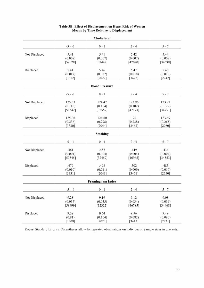
Table 3 contains the means of each of the four health outcome variables by

displacement status both before and after displacement. For women, we see that cholesterol is

the same on average for both groups pre-displacement but then it rises slightly for the

displaced but not for the non-displaced. Displaced women were slightly more likely to smoke

pre-displacement; then smoking probability falls for the non-displaced but increases for the

displaced. This table is suggestive; however, since these are just raw means, the numbers

could be influenced by compositional shifts.

The regression-based difference-in-differences estimates are in Table 4. In addition to

the four health variables considered earlier, we add estimates here for sickness benefit,

disability benefit, body mass index, and an alternative heart risk index (the Westerlund risk of

cardiovascular disease) that is a relative rather than an absolute index (see the appendix for

details). The estimates are consistent with the year-by-year regression results: among men,

there is very little evidence of a negative effect of displacement on any of the health measures

other than smoking, and as before, the smoking effect persists over time. Among women, we

15 The smoking estimates come from linear probability model. We have verified that the marginal effects and associated standard errors from a probit model are almost identical.

19

also find an effect on smoking. In addition, there is evidence that displacement leads to

higher cholesterol; there is no evidence of any effect on any of the other indicators.16

Robustness Checks

We next report the findings from a variety of different robustness checks. For brevity,

we only report estimates for the Framingham index as the dependent variable. However,

results using other outcomes were also robust to these checks.

Effect by Type of Displacement Event

While a job displacement is a very specific event, we next look at whether the

underlying cause of the displacement affects the magnitude of our findings, as it is quite

likely that the exact nature of a displacement event matters for health. These estimates are in

Table 5. One distinction we make is between those individuals who lose jobs due to a

downsizing and those who lose jobs because their plant closes. When we split the sample into

these two groups, it is clearly the case that the negative effects of a plant closure dominate

that of a downsizing with the differences being particularly large for women.

Some workers are displaced but transfer to another plant in the same firm (there are

4191 of these cases for men, 1320 for women). One might expect that these workers have a

much less stressful experience than other displaced workers so we report estimates in Table 5

where they are omitted from the sample. As expected, the effects of displacement are larger

16 Appendix Table 2 lists the coefficient estimates for the control variables for the regression in which the Framingham index is the dependent variable (Table 4). One interesting coefficient is that on pre-displacement earnings. Ignoring the endogeneity of earnings, the coefficient of -.135 for men implies that a 10% increase in average earnings reduces heart risk by just over 0.001 of a point. Displacement reduced earnings of men by about 6% in time periods 2 – 4 and this would then imply an earnings effect on heart risk that is quite tiny. The coefficient on earnings in the female regression is small and statistically insignificant. If the OLS effect of earnings is reasonable, it suggests that earnings losses are not an important channel in the decrease in health from displacement for either men or women.

20

here than in Table 3 for both men and women and now are statistically significant for men in

each of the 3 post-displacement periods.

Finally, to select a group that may be particularly adversely affected, we restrict the

treatment group to persons whose plant closed and who did not move to another plant in the

same firm (keeping the control group the same). The estimates are in the last row of Table 5.

We now see strong evidence of health impacts for both men and women and they appear to

persist for years after displacement. The magnitudes here are also significant at about a third

of a standard deviation for men and close to a full standard deviation effect for women.

Alternative Control Groups

Our baseline control group includes all individuals who are not displaced over the

benchmark 13-year period. As such, it includes individuals who are in firms that are

downsized but who are not themselves displaced. It is reasonable to believe, however, that

being in a plant that experienced a large downsizing may increase workloads and stress levels

for those who remain, thus having negative impacts on measured health. Therefore, we report

estimates where this group is excluded from the analysis (Control Group 2).

Those who are separated from their jobs but not a part of a mass displacement are also

included in the baseline control groups. One might be concerned that these individuals are

very different from those who are displaced and, as such, not appropriate for the control

group. As a robustness check, we also report estimates in which these people are omitted

from the sample (Control Group 3).17

The results with these alternative control groups are presented in Appendix Table 3.

Importantly, the estimates change very little when stayers from downsizing firms are

excluded from the control group (Control Group 2) but the displacement effects increase

17 While separators are excluded, Control Group 3 includes persons from downsizing firms who are not displaced.

21

when non-displaced separators are excluded from the control group. Overall, the estimates

appear quite robust to the choice of control group.

Using the Propensity Score

As is typically the case in displacement studies, we saw that there are systematic

differences between some characteristics of the treatment and control groups (Table 1). An

alternative to the regression approach is to use propensity score matching. We implement two

variants of this in conjunction with the regression analysis.18 First, we use the estimated

propensity score to reweight observations so that the weighted probability of displacement is

the same in both the treatment and control groups. We then report regression estimates using

these weights. Second, as suggested by Angrist and Pischke (2009), we use the estimated

propensity score as a pre-screen in the regression analysis. Intuitively, we exclude

observations with outlier values of the propensity score and check the robustness of our

regression estimates to this exclusion. Note that a limitation of the propensity score approach

is that we do not know pre-displacement health for persons whose health is measured post-

displacement. Therefore, we cannot use health information in forming the propensity score.

Because displacement is a fairly random event, even our rich set of control variables

have little explanatory power for whether a person is displaced at base year. For men, the

pseudo R2 from a logit regression is only 0.03.19 Education has a statistically significant but

small negative effect in that an extra year of education reduces the probability of

displacement by 0.002. Being a native Norwegian reduces the probability of displacement by

0.02, and an extra centimeter of height at age 18 reduces the probability of displacement by a

statistically significant but tiny .0006. Surprisingly, there is a small positive relationship

between cognitive test scores at age 18 and displacement. Displacements are more likely in

18 We revert to our original treatment and control groups for the propensity score analysis. 19 This logit regression included the same set of controls that we use in the main analysis.

22

bigger plants and there is the expected quadratic relationship between tenure and

displacement probability. There is no evidence of any relationship between BMI, lagged

average earnings, 1-digit industry, month of birth, family size, birth order, marital status, or

age on displacement probability for men. The results for women are generally similar.

Panel 3 of Appendix Table 2 shows regression estimates where observations have

been weighted using the estimated propensity score. Panels 4 and 5 show unweighted

estimates where the propensity score has been used to pre-screen observations; observations

with extreme values of the score have been omitted from the regression.20 Both of these

methods give estimates that are similar to the baseline difference-in-differences estimates

from Table 4.

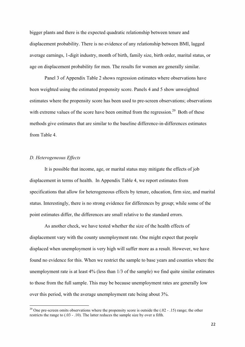
D. Heterogeneous Effects

It is possible that income, age, or marital status may mitigate the effects of job

displacement in terms of health. In Appendix Table 4, we report estimates from

specifications that allow for heterogeneous effects by tenure, education, firm size, and marital

status. Interestingly, there is no strong evidence for differences by group; while some of the

point estimates differ, the differences are small relative to the standard errors.

As another check, we have tested whether the size of the health effects of

displacement vary with the county unemployment rate. One might expect that people

displaced when unemployment is very high will suffer more as a result. However, we have

found no evidence for this. When we restrict the sample to base years and counties where the

unemployment rate is at least 4% (less than 1/3 of the sample) we find quite similar estimates

to those from the full sample. This may be because unemployment rates are generally low

over this period, with the average unemployment rate being about 3%.

20 One pre-screen omits observations where the propensity score is outside the (.02 - .15) range; the other restricts the range to (.03 - .10). The latter reduces the sample size by over a fifth.

23

E. Intent-to-treat Estimates

One concern with the previous estimates is that, when a plant is downsizing, it may

systematically choose to lay off the least healthy employees, as they are also likely to be less

productive.21 Additionally, firms sometimes seek voluntary layoffs when downsizing and

persons who volunteer to be displaced may be less healthy. The similarity of health before the

base year of displaced and non-displaced workers suggests that this is not a big issue but does

not rule it out altogether.

We follow the previous literature in addressing this point by including non-displaced

employees from downsizing firms in the treatment group (Sullivan and von Wachter, 2009).

In effect, this defines the treatment at the firm level. Note that, in addition to the possible

selection issue described above, it is possible that our estimates change because displacement

has a negative (or positive) effect on stayers in downsizing firms. A negative effect could

arise if the employment reduction increased the workload and stress of remaining employees,

a positive effect could arise if the displacement reduced uncertainty and made remaining

workers confident that the firm would now be viable and their jobs remain safe. Sullivan and

von Wachter (2009) refer to estimates using the firm-level definition of displacement as

“intent-to-treat” estimates.

The “intent-to-treat” estimates are in Table 6. If non-displaced workers are unaffected

by downsizings, we would expect estimates to be a bit smaller than earlier as the treatment

group now contains both affected and unaffected people. However, in general, the estimates

are quite similar to the estimates where only displaced workers are included in the treatment

group, suggesting that workers in affected firms may also bear the cost of the firm

21 This would be despite the fact that it is illegal to lay off workers based on their health status.

24

downsizing, even if they themselves are not displaced. We have looked at this question

directly by comparing the outcomes of non-displaced persons in downsizing firms to those

who are not displaced and are not in downsizing firms. Interestingly, we find that there is an

increase in smoking probability of about .05 at the time of downsizing but the effect

disappears after t=1. There are indications that the health of persons in downsizing firms

actually improves in the longer term as cholesterol and the heart risk index actually fall after

t=1. These estimates are consistent with the immediate effects of a displacement event being

stressful for all employees but the longer term health effects on the “survivors” being

positive. For women, there is no evidence of any health effects of downsizing on the non-

displaced population.

F. Cross-Effects

Finally, we have also examined whether displacement has any effect on the health of

spouses. Perhaps unsurprisingly given the small health effects on the individual who is

directly affected, we have found no evidence that the health of spouses is affected. This is

true when either the male or the female is the displaced worker.

7. Conclusion

Firm expansion and contraction are key elements to a well-functioning economy.

However, the process is not costless. Much of the recent research has focused on the

financial costs that are faced by workers, demonstrating the significant and potentially long-

lasting effects of job displacement. However, much less is known about the health effects of

these types of labor market shocks.

Using rich, detailed health data from Norway matched to administrative register data,

we show that job displacement has a significant effect on cardiovascular health around age

40. Importantly, this is almost entirely explained by changes in individual health behaviors;

25

smoking increasing significantly for both men and women immediately after displacement.

Interestingly, there is no equivalent health effect on the spouses of these workers.

In general the effects we find are quite small; however, as one might expect, the

health consequences of displacement are larger for those hardest hit--the subset of workers

whoso plants close and whose next job is not in another plant in the same firm. Among these

workers, we find substantial negative health effects for both men and women. In addition,

individuals from firms who downsize but who are not themselves laid off also experience a

negative health shock; however, this shock appears short-lived and there is some evidence

that they may actually have better health in the longer run.

26

References Anderson, K. M., P. M. Odell, P. W. Wilson, and W. B. Kannel. 1991. “Cardiovascular Disease Risk

Profiles.” Am Heart J., 121(1 Pt 2):293-8. Angrist, Joshua D., and Jörn-Steffen Pischke. 2009. Mostly Harmless Econometrics: An Empiricists

Companion. Princeton: Princeton University Press. Asgeirsdottir, Tinna Laufey, Hope Corman, Kelly Noonan, Torhildur Olafsdottir, Nancy E.

Reichman. 2012. “Are Recessions Good for Your Health Behaviors? Impacts of the Economic Crisis in Iceland.” NBER Working Paper #18233.

Bergemann, Annette, Erik Gronqvist, and Soffia Gudbjornsdottir, 2011. “The Effects of Job

Displacement on the Onset and Progression of Diabetes.” Netspar discussion paper 03/2011. Bjartveit K. 1986. “Effect of intervention on coronary heart disease risk factors in some Norwegian

counties.” Am J Med, 80(2A):12-7. Bosma, H., Peter, R., Siegrist, J., and M. Marmot. 1998. “Two Alternative Job Stress Models and the

Risk of Coronary Heart Disease.” American Journal of Public Health, 88: 68-74. Browning, Martin, Anne Danø Møller, and Eskil Heinesen. 2006. “Job displacement and stress-

related health outcomes.” Health Economics, 15: 1061–1075. Browning, Martin and Eskil Heinesen (2012). “The effect of job loss due to plant closure on

mortality and hospitalization.” Journal of Health Economics, 31: 599-616. Burda, Michael C., and Antje Mertens. 2001. “Estimating wage losses of displaced workers in

Germany.” Labour Economics, 8, 15–41. Carneiro, Anabela, and Pedro Portugal. 2006. “Earnings Losses of Displaced Workers: Evidence

from a Matched Employer-employee Data Set.” CETE Discussion Paper No. 0607. Cronbach, Lee J. 1964. Essentials of Psychological Testing, 2nd Edition. London, UK: Harper and

Row. Eliason, Marcus and Donald Storrie. 2004. “The Echo of Job Displacement.” ISER Working Paper

2004-20, Institute for Social and Economic Research. Eliason, Marcus and Donald Storrie. 2009a. “Job Loss is Bad for your Health – Swedish Evidence on

Cause-Specific Hospitalization following Involuntary Job Loss.” Social Science and Medicine, 68: 1396-1406.

Eliason, Marcus and Donald Storrie. 2009b. “Does Job Loss shorten Life?” Journal of Human

Resources, 44(2): 277-302. Falba, T., H. M. Teng, J. L. Sindelar, and W. T. Gallo. 2005. ‘‘The Effect of Involuntary Job Loss on

Smoking Intensity and Relapse.’’ Addiction 100(9):1330–9. Farber, Hank S. 2005. “What Do We Know About Job Loss in the U.S.? Evidence from the

Displaced Workers Survey, 1984–2004.” Economic Perspectives. 2005;2Q:13–28.

27

Gallo, William T., Elizabeth H. Bradley, and Stanislav V. Kasl. 2001. "The effect of job

displacement on subsequent health." Quarterly Journal of Economic Research, 70:159-65. Gallo, William T. Elizabeth H. Bradley, Tracy A. Falba, Joel A. Dubin, Laura D. Cramer, Sidney T.

Bogardus Jr., and Stanislav V. Kasl. 2004. “Involuntary Job Loss as a Risk Factor for Subsequent Myocardial Infarction and Stroke: Findings from the Health and Retirement Survey.” American Journal of Industrial Medicine, 45:408–416.

Hildreth, Andrew K. G., Till von Wachter, and Weber Handverker. 2008. "Estimating the 'True' Cost

of Job Loss: Evidence Using Matched Data from California 1991-2000." Memo, Columbia University.

Huttunen, Kristiina, Jarle Møen, and Kjell G. Salvanes. 2011. “How Destructive is Creative Destruction? Effects of Job Loss on Job Mobility, Withdrawal, and Income” Journal of the European Economic Association. 9 (5): 840 - 870.

Jacobson, Louis S, Robert J. LaLonde, Daniel Sullivan. 1993. “Earnings Losses of Displaced

Workers.” American Economic Review, 83:685–709. Jacobsen B.K., I. Stensvold, K. Fylkesnes, I. S. Kristiansen, G. S. Thelle. 1992. “The Nordland

health study”, Scandinavian Journal of Social Medicine, 20 (3): 184-7. Kivimäki, M., Leino-Arjas, P., Luukkonen, R., Riihimäki, H., Vahtera, J. and Kirjonen, J. 2002.

“Work Stress and Risk of Cardiovascular Mortality: Prospective Cohort Study of Industrial Employees.” British Medical Journal, 325:857-861.

Kuhn, Andreas, Rafael Lalive, and Josef Zweimfiller. 2007. "The Public Health Costs of

Unemployment," Cahiers de Recherches Economiques du Departement d'Econometrie et d'Economie politique07.08, University de Lausanne, Faculte des HEC.

Marcus, Jan. 2012. “Does Job Loss Make You Smoke and Gain Weight?” mimeo, January. Martikainen, Pekka, Netta Maki, and Markus Jantti. 2007."The Effects of Unemployment on

Mortality Following Workplace Downsizing and Workplace Closure: A Register-Based Follow-Up Study of Finnish Men and Women during Economic Boom and Recession," American Journal of Epidemiology, 165:1070-1075.

Morris, JK, D.G Cook. 1991. “A critical review of the effect of factory closures on health.” Br J Ind

Med, 48: 1–8. Møen, Jarle, Kjell G. Salvanes and Erik Ø. Sørensen. 2003. “Documentation of the Linked

Empoyer Employee Data Base at the Norwegian School of Economics,” Mimeo, The Norwegian School of Economics and Business Administration.

Nystad W., H.E. Meyer, P. Nafstad, A.Tverdal, A. Engeland. 2004. “Body mass index in relation to

adult asthma among 135,000 Norwegian men and women.”American Journal of Epidemiology, 160(10) :969-76.

28

Page, Marianne, Phil Oreopoulos, and Ann Stevens. 2008. “The Intergenerational Effects of Worker Displacement.” Journal of Labor Economics, 26(3):455-484.

Rege, Mari, Torbjrøn Skardhamar, Kjetil Telle, Mark Votruba. 2009a. “Job Loss and Crime.”

Discussion Paper No. 593, Research Department, Statistics Norway. Rege, Mari, Kjetil Telle, and Mark Votruba. 2009b. “The Effect of Plant Downsizing on Disability

Pension Utilization.” Journal of the European Economic Association, 7(4):754–785. Rege, Mari, Kjetil Telle, Mark Votruba.2011. ”Parental Job Loss and Children's School

Performance.” Review of Economic Studies, 78: 1462-1489. Ruhm Christopher. 2000. “Are recessions good for your health?” Quarterly Journal of Economics,

115(2): 617-650. Ruhm, Christopher. 2005. “Healthy Living in Hard Times.” Journal of Health Economics,

24(2):341-63. Salm, Martin. 2009. “Does Job Loss Cause Ill Health?” Health Economics, 18(9), 1075-1089. Sullivan, Daniel and Till von Wachter. 2009. “Job Displacement and Mortality: An Analysis Using

Administrative Data.” Quarterly Journal of Economics, 124 (3): 1265-1306. Strully, Kate W. 2009. “Job Loss and Health in the U.S. Labor Market.” Demography, 46(2): 221-

246. Sundet, Martin Jon, Dag G. Barlaug, and Tore M. Torjussen. 2004. "The End of the Flynn Effect? A

Study of Secular Trends in Mean Intelligence Test Scores of Norwegian Conscripts During Half a Century." Intelligence , XXXII: 349-362.

Sundet, Jon Martin, Kristian Tambs, Jennifer R. Harris, Per Magnus, and Tore M. Torjussen.2005.“

Resolving the Genetic and Environmental Sources of the Correlation Between Height and Intelligence: A Study of Nearly 2600 Norwegian Male Twin Pairs.” Twin Research and Human Genetics, VII: 1-5.

Søgaard, A. J. 2006. “Cohort Norway (CONOR). Materials and methods.” memo, Norwegian

Institute of Public Health. Søgaard, A. J., R. Selmer, E. Bjertnes, G. D. Thelle. 2003. “The Oslo Health Study. The impact of

Self-selection in a Large, Populations-based Survey.” 2003. International Journal of Equity in Health, 3(3): 3-13.

Søgaard, A. J., I. Bjelland, G. S. Thelle, and E. Røysamb. 2003. “A comparison of the CONOR

Mental Health Index to the HSCL-10 and HADS Measuring mental health status in The Oslo Health Study and the Nord-Trøndelag Health Study.” Norsk Epidemiologi, 13(2): 279-284.

Thrane, Vidkunn Coucheron. 1977. “Evneprøving av Utskrivingspliktige i Norge 1950-53,”

Arbeidsrapport nr. 26, INAS.

29

Von Wachter, Till, and Stefan Bender. 2006. "In the Right Place at the Wrong Time: The Role of Firms and Luck in Young Workers' Careers." American Economic Review, 96(5): 1679–1705.

30

Table 1: Means by Displacement Status (At time 0) MEN

Variable

Displaced Not Displaced P value for difference

Age 41.31 (0.04)

41.26 (0.01)

0.34

Education 11.10 (0.05)

11.27 (0.01)

<0.01

IQ Score 5.89 (0.05)

5.82 (0.01)

0.11

Tenure 7.23 (0.09)

8.64 (0.02)

<0.01

Height (at 18) 178.57 (0.16)

178.93 (0.04)

0.02

BMI (at 18) 21.32 (0.06)

21.51 (0.01)

<0.01

Lagged Earnings 12.51 (0.006)

12.52 (0.002)

0.25

Plant Size at 0 265.02 (7.74)

245.32 (2.05)

0.02

Family Size 2.91 (0.03)

2.92 (0.01)

0.84

Birth Order 1.70 (0.02)

1.71 (0.005)

0.55

Native 0.96 (0.004)

0.97 (0.001)

<0.01

Married 0.77 (0.01)

0.77 (0.002)

0.86

Months Unemployed at -1 0.08 (0.01)

0.04 (0.002)

<0.01

Number of Observations 3019 46455

31

Table 1: Means by Displacement Status (At time 0) WOMEN

Variable

Displaced Not Displaced P value for difference

Age 41.17 (0.09)

41.26 (0.02)

0.34

Education 10.43 (0.07)

10.61 (0.02)

<0.01

Tenure 6.13 (0.15)

7.15 (0.04)

<0.01

Lagged Earnings 12.08 (0.01)

12.15 (0.003)

<0.01

Plant Size at 0 183.62 (10.41)

204.45 (3.53)

0.14

Family Size 2.97 (0.05)

2.97 (0.01)

0.87

Birth Order 1.78 (0.04)

1.75 (0.01)

0.46

Native 0.97 (0.005)

0.97 (0.001)

0.95

Married 0.67 (0.01)

0.67 (0.004)

0.81

Months Unemployed at -1 0.10 (0.01)

0.04 (0.003)

<0.01

Number of Observations 1047 15773

32

Table 2A: Effect of Displacement on Outcomes (Men) Time Cholesterol Blood Pressure Smoking Framingham Index -5 .033

(.035) [24931]

-.223 (.435)

[25130]

-.001 (.016)

[25163]

.035 (.100)

[24927]

-4 -.064** (.031)

[29060]

.166 (.385)

[29246]

.001 (.014)

[29299]

-.084 (.088)

[29056]

-3 .005 (.026)

[34258]

-.315 (.297)

[34425]

.003 (.011)

[34497]

0.002 (.073)

[34238]

-2 .017 (.025)

[39256]

-.056 (.290)

[39413]

.014 (.011)

[39488]

.074 (.069)

[39219]

-1 .019 (.023)

[43196]

.084 (.282)

[43337]

.013 (.010)

[43403]

0.101 (.066)

[43135]

0 .011 (.020)

[49185]

.343 (.259)

[49341]

.017** (.009)

[49352]

.129** (.059)

[49063]

1 .013 (.019)

[54304]

.062 (.235)

[54473]

.023** (.008)

[54364]

.121** (.055)

[54053]

2 .003 (.018)

[55103]

.115 (.233)

[55256]

.021** (.008)

[55181]

.109** (.054)

[54874]

3 .044** (.019)

[53670]

.102 (.221)

[55825]

.038** (.008)

[53734]

.242** (.052)

[53427]

4 .029 (.018)

[49184]

-.147 (.215)

[49203]

.023** (.008)

[49116]

.136** (.052)

[48949]

5 .004 (.019)

[44851]

-.296 (.233)

[44826]

.040** (.009)

[44725]

.209** (.056)

[44610]

6 -.005 (.020)

[40248]

.107 (.241)

[40220]

.007 (.009)

[40099]

-.009 (.056)

[40011]

7 -.003 (.020)

[34515]

.227 (.258)

[34488]

.026** (.009)

[34366]

.135** (.060)

[34285] All coefficients come from separate regressions with the full set of control variables. The control variables include base year dummies, survey dummies, survey month dummies, age at health measurement, a dummy for whether the person is married in the base year, years of education at the base year, birth order dummies, dummies for number of siblings, IQ test score at age 18, height at age 18, a quadratic in BMI at age 18, a dummy variable for whether the person was born in Norway, month of birth dummies, plant size in the base year (number of employees), a quadratic in tenure in the base year, the average of the log real earnings from t =

33

-5 to t = -1, dummies for county of residence in the base year, 1-digit industry dummies for the base year industry. Displacement occurs between 0 and 1. Robust Standard Errors in Parentheses. * implies statistically significant at the 10% level; ** implies statistically significant at the 5% level.

34

Table 2B: Effect of Displacement on Outcomes (Women)

Time Cholesterol Blood Pressure Smoking Framingham Index -5 -.002

(.049) [9512]

-.600 (.624) [9578]

.002 (.024) [9581]

-.029 (.226) [9511]

-4 .046 (.042)

[11154]

-.132 (.573)

[11217]

.028 (.021)

[11222]

.244 (.192)

[11152]

-3 -.039 (.037)

[12587]

.043 (.518)

[12647]

.010 (.019)

[12652]

-.085 (.176)

[12583]

-2 .007 (.036)

[14033]

.452 (.519)

[14102]

.011 (.018)

[14103]

.165 (.173)

[14026]

-1 -.036 (.034)

[15054]

-.254 (.494)

[15128]

-.011 (.018)

[15118]

-.138 (.163)

[15036]

0 .010 (.031)

[16744]

-.294 (.419)

[16809]

.015 (.016)

[16773]

.141 (.145)

[16697]

1 .068** (.032)

[17725]

-.075 (.444)

[17792]

.034** (.016)

[17729]

.413** (.149)

[17648]

2 .042 (.032)

[17607]

.216 (.427)

[17667]

.053** (.015)

[17600]

.480** (.143)

[17528]

3 .024 (.030)

[17296]

.283 (.401)

[17379]

.016 (.014)

[17302]

.107 (.139)

[17212]

4 .080** (.032)

[15542]

-.683 (.428)

[15589]

.030** (.015)

[15514]

.270* (.142)

[15457]

5 .033 (.031)

[13964]

-.425 (.444)

[13988]

.024 (.016)

[13916]

.210 (.148)

[13882]

6 .016 (.034)

[12479]

-.908* (.416)

[12503]

.012 (.017)

[12433]

.046 (.156)

[12401]

7 .045 (.037)

[10998]

-1.10** (.486)

[11028]

.013 (.018)

[10954]

.080 (.168)

[10916] All coefficients come from separate regressions with the full set of control variables. The control variables are the same as in Table 2A. Displacement occurs between 0 and 1. Robust Standard Errors in Parentheses. * implies statistically significant at the 10% level; ** implies statistically significant at the 5% level.

35

Table 3A: Effect of Displacement on Heart Risk of Men Means by Time Relative to Displacement

Cholesterol

-5 - -1

0 - 1

2 - 4

5 - 7

Not Displaced 5.81

(0.005) [161738]

5.80 (0.005) [97016]

5.78 (0.005)

[146409]

5.78 (0.005)

[109877]

Displaced 5.81 (0.012) [8963]

5.82 (0.013) [6473]

5.83 (0.010) [11548]

5.79 (0.011) [9737]

Blood Pressure

-5 - -1

0 - 1

2 - 4

5 - 7

Not Displaced 135.23

(0.066) [162552]

134.40 (0.059) [97307]

133.92 (0.057)

[146675]

133.55 (0.066)

[109804]

Displaced 135.01 (0.141) [8999]

134.79 (0.170) [6507]

133.94 (0.126) [11609]

133.84 (0.137) [9730]

Smoking

-5 - -1

0 - 1

2 - 4

5 - 7

Not Displaced .412

(0.002) [162835]

.392 (0.002) [97209]

.383 (0.002)

[146432]

.367 (0.002)

[109467]

Displaced .422 (0.005) [9015]

.427 (0.006) [6507]

.426 (0.005) [11599]

.406 (0.005) [9723]

Framingham Index

-5 - -1

0 - 1

2 - 4

5 - 7

Not Displaced 7.57

(0.016) [161622]

7.42 (0.014) [96661]

7.34 (0.014)

[145742]

7.25 (0.015)

[109208]

Displaced 7.60 (0.030) [8953]

7.63 (0.040) [6455]

7.61 (0.030) [11508]

7.46 (0.032) [9698]

Robust Standard Errors in Parentheses allow for repeated observations on individuals. Sample sizes in brackets.

36

Table 3B: Effect of Displacement on Heart Risk of Women Means by Time Relative to Displacement

Cholesterol

-5 - -1

0 - 1

2 - 4

5 - 7

Not Displaced 5.41

(0.008) [59028]

5.41 (0.007) [32442]

5.42 (0.007) [47020]

5.44 (0.008) [34699]

Displaced 5.41 (0.017) [3312]

5.46 (0.022) [2027]

5.47 (0.018) [3425]

5.48 (0.019) [2742]

Blood Pressure

-5 - -1

0 - 1

2 - 4

5 - 7

Not Displaced 125.33

(0.110) [59342]

124.47 (0.104) [32557]

123.96 (0.102) [47173]

123.91 (0.122) [34751]

Displaced 125.06 (0.236) [3330]

124.60 (0.298) [2044]

124 (0.238) [3462]

123.69 (0.265) [2760]

Smoking

-5 - -1

0 - 1

2 - 4

5 - 7

Not Displaced .461

(0.004) [59345]

.457 (0.004) [32459]

.449 (0.004) [46965]

.434 (0.004) [34553]

Displaced .479 (0.010) [3331]

.498 (0.011) [2043]

.502 (0.009) [3451]

.485 (0.010) [2750]

Framingham Index

-5 - -1

0 - 1

2 - 4

5 - 7

Not Displaced 9.28

(0.037) [58999]

9.19 (0.035) [32322]

9.12 (0.034) [46785]

9.08 (0.039) [34468]

Displaced 9.38 (0.81) [3309]

9.64 (0.104) [2023]

9.56 (0.082) [3412]

9.49 (0.090) [2731]

Robust Standard Errors in Parentheses allow for repeated observations on individuals. Sample sizes in brackets.

37

Table 4A: Effect of Displacement on Heart Risk of Men

Difference-in-Difference Estimates with controls

Displaced Displaced* Period1

Displaced* Period2

Displaced* Period3

Dependent Variable Cholesterol (551761)

.003 (.013)

.006 (.018)

.021 (.016)

-.003 (.017)

Blood Pressure (553183)

-.063 (.155)

.223 (.222)

.067 (.192)

.044 (.206)

Smoking (552787)

.009 (.006)

.011 (.008)

.018** (.007)

.016** (.007)

Framingham Index (549847)

.042 (.037)

.077 (.051)

.114** (.045)

.075 (.048)

Sickness Benefit (536645)

.005** (.002)

.013** (.003)

.001 (.003)

.001 (.002)

Disability Benefit (535784)

-.001 (.001)

.001 (.001)

.002* (.001)

.002 (.002)

Body Mass Index (554440)

-.124 (.111)

-.109 (.215)

.163 (.191)

.379* (.229)

Alternative Index (536050)

.459 (.616)

1.42 (.90)

2.36** (.80)

.555 (.805)

Each row represents one regression. The control variables include base year dummies, survey dummies, survey month dummies, age at health measurement, a dummy for whether the person is married in the base year, years of education at the base year, birth order dummies, dummies for number of siblings, IQ test score at age 18, height at age 18, a quadratic in BMI at age 18, a dummy variable for whether the person was born in Norway, month of birth dummies, plant size in the base year (number of employees), a quadratic in tenure in the base year, the average of the log real earnings from t = -5 to t = -1, dummies for county of residence in the base year, 1-digit industry dummies for the base year industry. Displacement occurs between 0 and 1. Robust Standard Errors in Parentheses allow for repeated observations on individuals. Sample sizes in brackets. * implies statistically significant at the 10% level; ** implies statistically significant at the 5% level.

38

Table 4B: Effect of Displacement on Heart Risk of Women


Displaced Displaced*G1 Displaced*G2 Displaced*G3 Dependent Variable Cholesterol (184695)

-.003 (.019)

.038 (.028)

.048* (.025)

.036 (.027)


-.056 (.259)

-.193 (.381)

-.006 (.341)

-.606 (.371)

Smoking (184897)

.008 (.009)

.015 (.014)

.026** (.012)

.017 (.013)


.039 (.087)

.214 (.130)

.238** (.115)

.143 (.124)


.003 (.004)

.009 (.007)

.007 (.006)

-.001 (.006)


-.002 (.001)

.002 (.003)

.000 (.003)

.007 (.004)


-.125 (.211)

.551 (.539)

.407 (.427)

.277 (.514)


.106 (.126)

.110 (.179)

.472** (.181)

-.001 (.183)

Each row represents one regression. The control variables include base year dummies, survey dummies, survey month dummies, age at health measurement, a dummy for whether the person is married in the base year, years of education at the base year, birth order dummies, dummies for number of siblings, a dummy variable for whether the person was born in Norway, month of birth dummies, plant size in the base year (number of employees), a quadratic in tenure in the base year, the average of the log real earnings from t = -5 to t = -1, dummies for county of residence in the base year, 1-digit industry dummies for the base year industry. Displacement occurs between 0 and 1. Robust Standard Errors in Parentheses allow for repeated observations on individuals. Sample sizes in brackets. * implies statistically significant at the 10% level; ** implies statistically significant at the 5% level.

39

Table 5: Effects by Type of Displacement (Framingham Index only)


Men

Displaced Displaced*G1 Displaced*G2 Displaced*G3 Downsizings only (442394)

.045 (.048)

.019 (.068)

.069 (.060)

.042 (.065)

Plant Closings Only (438696)

.075 (.057)

.141* (.079)

.168** (.067)

.104 (.072)

Same Firm Displaced Excluded (545656)

.040 (.038)

.116** (.054)

.133** (.048)

.117** (.051)

Same Firm Displaced Excluded and Plant Closings Only (438045)

.050 (.059)

.173** (.080)

.192** (.070)

.136** (.074)

Women

Displaced Displaced*G1 Displaced*G2 Displaced*G3 Downsizings only (144512)

.110 (.118)

.128 (.176)

-.024 (.156)

-.045 (.171)

Plant Closings Only (143893)

-.086 (.134)

.328* (.193)

.535** (.168)

.390** (.179)

Same Firm Displaced excluded(183140)

.036 (.090)

.254* (.135)

.255** (.119)

.162 (.129)

Same Firm Displaced excluded and Plant Closings Only (143763)

-.111 (.136)

.413** (.195)

.542** (.170)

.430** (.182)


40

Table 6A: Intention to Treat Effects for Men


Displaced Displaced* Period1

Displaced* Period2

Displaced* Period3

Dependent Variable Cholesterol (495213)

.014 (.012)

.007 (.016)

-.007 (.015)

-.006 (.015)


-.063 (.149)

.440** (.206)

.173 (.179)

.254 (.189)

Smoking (495930)

.006 (.005)

.016** (.007)

.017** (.007)

.011* (.007)


.050 (.036)

.116** (.048)

.067 (.042)

.049 (.045)


.002 (.002)

.006** (.003)

.005** (.003)

.001 (.003)


.0001 (.001)

-.001 (.001)

-.0004 (.001)

-.001 (.001)


-.074 (.112)

-.049 (.200)

.076 (.174)

.432** (.207)


.684 (.603)

1.37* (.83)

1.70** (.75)

.749 (.749)


41

Table 6B: Intention to Treat Effects for Women


Displaced Displaced*G1 Displaced*G2 Displaced*G3 Dependent Variable Cholesterol (167566)

.003 (.018)

.011 (.025)

.030 (.023)

.011 (.024)


.395 (.248)

-.627 (.348)

-.145 (.318)

-.822** (.340)

Smoking (167688)

.007 (.009)

.012 (.013)

.026** (.011)

.016 (.012)


.100 (.083)

.109 (.118)

.191* (.106)

.059 (.112)


-.001 (.004)

-.001 (.006)

.004 (.005)

.007 (.006)


-.002* (.001)

.001 (.002)

-.004 (.003)

.002 (.004)


.295 (.225)

.544 (.490)

-.345 (.387)

-.262 (.477)


.093 (.116)

.003 (.159)

.367** (.158)

-.040 (1.66)


42

Appendix Table 1: Effect of Displacement on Labor Market Outcomes Men Women Time Log Earnings Whether Employed Log Earnings Whether Employed -5 0.000

(.009) [25110]

-0.041** (0.010) [25167]

-0.071** (.032) [9469]

-0.001 (0.014) [9582]

-4 0.000 (0.007) [29564]

-0.013* (0.007) [29303]

0.009 (0.016) [11119]

-0.031** (0.013) [11224]

-3 -0.001 (0.006) [33539]

-0.004 (0.005) [34517]

0.004 (0.012) [12577]

-0.015 (0.010) [12656]

-2 -0.006 (0.004) [39484]

-0.015** (0.005) [39525]

-0.019* (0.011) [14070]

-0.030** (0.010) [14110]

-1 -0.002 (0.002) [43456]

0.0002** (0.0001) [43464]

-0.014** (0.006) [15133]

0.0004* (0.0002) [15136]

0 -0.013** (0.005) [49474]

-

[49474]

-0.027** (0.013) [16820]

-

[16820]

1 -0.061** (0.008) [54525]

-0.178** (0.007) [54616]

-0.049** (0.016) [17729]

-0.176** (0.013) [17806]

2 -0.055** (0.007) [55185]

-0.106** (0.006) [55411]

-0.060** (0.018) [17493]

-0.125** (0.012) [17679]

3 -0.048** (0.008) [53615]

-0.073** (0.005) [53977]

-0.061** (0.019) [17087]

-0.076** (0.011) [17386]

4 -0.055** (0.009) [48918]

-0.076** (0.006) [49351]

-0.087** (0.024) [15245]

-0.077** (0.012) [15599]

5 -0.043** (0.010) [44448]

-0.063** (0.006) [44966]

-0.72** (0.026) [13609]

-0.051** (0.012) [13998]

6 -0.036** (0.010) [39827]

-0.057** (0.006) [40336]

-0.042** (0.026) [12098]

-0.067** (0.013) [12511]

7 -0.031** (0.011) [34071]

-0.041** (0.006) [34596]

-0.095** (0.034) [10562]

-0.081** (0.015) [11036]

All coefficients come from separate regressions with the full set of control variables. The control variables are the same as in Table 2. Displacement occurs between 0 and 1. Robust standard errors in parentheses. * implies statistically significant at the 10% level; ** implies statistically significant at the 5% level.

43

Appendix Table 2

Coefficients on Selected Other Variables

Dependent Variable is Framingham Index

Men Women

Married

-.363** (.026)

-.632** (.055)

Education -.182** (.005)

-.394** (.013)

Cognitive Score -.136** (.010)

Height -.030** (.003)

BMI -.027 (.068)

BMI Squared .002 (.001)

Native .461** (.077)

1.95** (.173)

Plant Size/1000 .010 (.028)

-.165** (.067)

Tenure -.009* (.005)

-.011 (.012)

Tenure Squared/100 -.005 (.025)

.074 (.065)

Prior Average Log Earnings -.135** (.038)

-.008 (.066)

N 521395 184049

Robust Standard Errors in Parentheses allow for repeated observations on individuals.

* implies statistically significant at the 10% level; ** implies statistically significant at the 5% level.

44

Appendix Table 3: Robustness Checks (Framingham Index only)

Men

Displaced Displaced*G1 Displaced*G2 Displaced*G3 Control Group 2 (486335)

.050 (.037)

.078 (.052)

.111** (.046)

.069 (.049)

Control Group 3 (332038)

.017 (.040)

.088 (.052)

.146** (.047)

.128** (.051)

Propensity Score Weighting (549847)

.042 (.037)

.078 (.052)

.118** (.046)

.069 (.049)

Propensity Score Screening (.02 - .15) (533367)

.035 (.037)

.086* (.052)

.107** (.047)

.076 (.050)


.029 (.041)

.064 (.059)

.089 (.054)

.053 (.059)

Women

Displaced Displaced*G1 Displaced*G2 Displaced*G3 Control Group 2 (164476)

.057 (.088)

.220* (.130)

.237** (.116)

.115 (.125)

Control Group 3 (116652)

.058 (.092)

.211 (.132)

.249** (.119)

.125 (.130)

Propensity Score Weighting (184044)

.060 (.087)

.214 (.131)

.202* (.117)

.076 (.125)


.033 (.088)

.252* (.132)

.263** (.118)

.150 (.127)


.040 (.098)

.293** (.147)

.396** (.136)

.033 (.148)


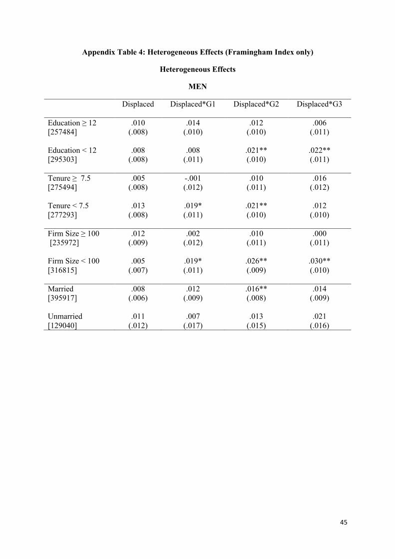
45

Appendix Table 4: Heterogeneous Effects (Framingham Index only)

Heterogeneous Effects

MEN

Displaced Displaced*G1 Displaced*G2 Displaced*G3 Education ≥ 12 [257484]

.010 (.008)

.014 (.010)

.012 (.010)

.006 (.011)

Education < 12 [295303]

.008 (.008)

.008 (.011)

.021** (.010)

.022** (.011)

Tenure ≥ 7.5 [275494]

.005 (.008)

-.001 (.012)

.010 (.011)

.016 (.012)

Tenure < 7.5 [277293]

.013 (.008)

.019* (.011)

.021** (.010)

.012 (.010)

Firm Size ≥ 100 [235972]

.012 (.009)

.002 (.012)

.010 (.011)

.000 (.011)

Firm Size < 100 [316815]

.005 (.007)

.019* (.011)

.026** (.009)

.030** (.010)

Married [395917]

.008 (.006)

.012 (.009)

.016** (.008)

.014 (.009)

Unmarried [129040]

.011 (.012)

.007 (.017)

.013 (.015)

.021 (.016)

46

WOMEN

Displaced Displaced*G1 Displaced*G2 Displaced*G3 Education ≥ 12 [54407]

-.042 (.170)

.352 (.255)

.154 (.224)

-.108 (.236)

Education < 12 [129642]

.052 (.101)

.167 (.151)

.270** (.135)

.222 (.147)

Tenure ≥ 7.5 [71516]

.117 (.139)

-.032 (.225)

.138 (.205)

.121 (.236)

Tenure < 7.5 [112533]

.000 (.111)

.333** (.163)

.274* (.144)

.141 (.151)

Firm Size ≥ 100 [68406]

.072 (.147)

.190 (.219)

.146 (.198)

.057 (.209)

Firm Size < 100 [115643]

.035 (.108)

.206 (.163)

.267* (.143)

.195 (.156)

Married [116152]

.016 (.106)

.342** (.161)

.135 (.144)

.127 (.164)

Unmarried [61350]

.073 (.151)

-.019 (.223)

.392* (.203)

.133 (.212)


47

Appendix: Heart Risk Indices

Framingham Risk Score

To calculate the risk score we use the scale for persons aged 40-49 as most people in our sample are in this age range. Also, we exclude age as a risk factor. We do not have information on HDL cholesterol for most of the sample so we exclude this variable. We assume that people are not having treatment for high blood pressure. Our version of the Framingham risk score is calculated as follows:

Framingham Risk Score for Women

Total cholesterol, mg/dL: Under 160: 0 points. 160-199: 3 points. 200-239: 6 points. 240-279: 8 points. 280 or higher: 10 points.

If cigarette smoker: 7 points. All non smokers: 0 points.

Systolic blood pressure, mm Hg: Under 120: 0 points. 120-129: 1 point. 130-139: 2 points. 140-159: 3 points. 160 or higher: 4 points.

Framingham Risk Score for Men

Total cholesterol, mg/dL: Under 160: 0 points. 160-199: 3 points. 200-239: 5 points. 240-279: 6 points. 280 or higher: 8 points. If cigarette smoker: 5 points.

All non smokers: 0 points. Systolic blood pressure, mm Hg: Under 120: 0 points. 120-129: 0 points. 130-139: 1 point. 140-159: 1 point. 160 or higher: 2 points. The point score translates into an estimate of the probability of future coronary heart disease events with higher scores indicating higher probability of disease. For example, for men, 5 points corresponds to approximately a 2% 10-year risk, 10 points indicates 6%, and 15 points indicates 20%. Equivalent figures for women are <1%, 1%, and 3%.

Westerlund risk of cardiovascular disease

This variable measures the risk of cardiovascular disease over the next 10 years. The scale is relative to a woman with zero risk characteristics. The mean score for men is 35 which means the average man is 35 times more likely to have cardiovascular disease than a woman with low risk characteristics. The lowest value of 1 is allocated to females who have

1. Systolic Blood Pressure less than 135 2. Non-smoker 3. No family history of heart disease 4. Cholesterol less than 4.91

In contrast, a man with

48

1. Systolic Blood pressure of 148 2. Smokes 10 cigarettes a day 3. No family history of heart disease 4. Cholesterol of 5.95

Would have a score of 5*2*2.5*1*2 = 50. Note that this scale is a multiplicative function of blood pressure, smoking behavior, family history of heart disease, and cholesterol. This score has been shown to have an approximately linear relationship with the incidence of death from heart disease in Norway.

Documents

Losing Heart? The Effect of Job Displacement on Health