Loss-of-Control: Perspectives on Flight Dynamics and

Control of Impaired Aircraft

Harry G. Kwatny ∗, Jean-Etienne T. Dongmo †, Robert C. Allen ‡ and Bor-Chin Chang §

Drexel University, 3141, Chestnut Street, Philadelphia, PA, 19104.

Gaurav Bajpai ¶

Techno-Sciences, Inc., 11750 Beltsville Road, Beltsville, MD, 20705.

Loss-of-Control (LOC) is a major factor in fatal aircraft accidents. Although definitionsof LOC remain vague in analytical terms, it is generally associated with a significantlydiminished capability of the pilot to control the aircraft. In previous work we consideredhow the ability to regulate an aircraft deteriorates around stall points. In this paper weexamine how damage to control effectors impacts the capability to keep the aircraft withinan acceptable envelope and to maneuver within it. We show that even when a sufficientset of steady motions exist, the ability to regulate around them or transition between themcan be difficult and nonintuitive, particularly for impaired aircraft.

Nomenclature

x State vectory Measurementsz Regulated variablesµ System parametersu Control inputsα Angle of attack, degβ Side slip angle, degV Velocity, ft/sX x inertial coordinate, ftY y inertial coordinate, ftZ z inertial coordinate, ftp x body-axis angular velocity component, deg/sq y body-axis angular velocity component, deg/sr z body-axis angular velocity component, deg/su x body-axis translational velocity component, ft/sv y body-axis translational velocity component, ft/sw z body-axis translational velocity component, ft/sφ Euler roll angle, degθ Euler pitch angle, degψ Euler yaw angle, degΨ Heading, degγ Flight path angle, degA System matrix of a linear systemB Control matrix of a linear system

∗S. Herbert Raynes Professor, AIAA Member†Graduate Student, AIAA Student Member‡Graduate Student, AIAA Student Members§Professor, AIAA Member¶Director, Dynamics and Control, AIAA Member

1 of 11

American Institute of Aeronautics and Astronautics

C Output matrix of a linear systemT Thrust, lbfδe elevator input, degδa Aileron input, degδr Rudder input, degC envelopeS safe setU control constraint setT trim manifold

I. Introduction

There is ample evidence indicating that Loss-of-Control (LOC) is a major factor in fatal aircraft accidents(for example, [1–3]). While definitions of LOC remain vague in analytical terms,4,5 it is generally

associated with flight outside the normal flight envelope, nonlinear behaviors and, most importantly, withan inability of the pilot to control the aircraft. In previous work6,7 we considered how controllability andthe ability to regulate an aircraft deteriorate around static bifurcation (stall) points. It was shown that thecorrect control strategies in neighborhoods of these points could change abruptly, contributing to confusionand with the consequent possibility of inappropriate pilot inputs. In [7], we also illustrated how controlbounds can effect the ability of a pilot to keep the aircraft within its admissible flight envelope whichordinarily excludes such bifurcation points.

In this paper we further examine the issues associated with keeping the aircraft, unimpaired or impaired,within its prescribed envelope and the extent to which it can maneuver within it. Loosely stated, there arefour basic questions:

1. Is it possible to keep the aircraft within its flight envelope?

2. Can the aircraft maneuver satisfactorily within the envelope?

3. How can departure from it be prevented?

4. How can the aircraft state be restored to the envelope in the event that it departs from it?

Here we focus on the first two questions. The first question can be addressed in terms of the concept ofa safe set or viable set .8,9 Safe set theory could be used as a basis for envelope protection and prevention ofsome forms of LOC, but this idea has not been fully developed. The idea of a safe set derives from a decadesold control problem in which the plant controls are restricted to a bounded set U and it is desired to keepthe system state within a convex, not necessarily bounded, subset C of the state space. Feuer and Heyman10

studied the question: under what conditions does there exist for each initial state in C an admissible controlproducing a trajectory that remains in C for all t > 0? When C does not have this property we try to identifythe safe set, S, that is, the largest subset of C that does. Clearly, if we wish the aircraft to remain in C, wemust insure that it remains in S.

We would also like to know how the aircraft can maneuver within S. Controlled flight requires theexistence of a suitable set of steady motions and the ability to smoothly transition between them. Thismeans that we need to understand the equilibrium point structure within S and we need to identify anyimpediments to regulating around them or steering from one to another. These questions are examined inthis paper.

Ordinarily, if a an aircraft is impaired we expect that the safe set will shrink. We will show that theequilibrium point structure within the reduced safe set changes as well and the ability to maneuver issignificantly diminished. Furthermore, control strategies required to execute transition maneuvers and toregulate around steady motions may be complex and non-intuitive. We suggest this as another mechanismof LOC. Examples are based on NASA’s Generic Transport Model (GTM).11

The organization of the paper is as follows. In Section II we discuss the GTM and the mathematicalmodels we use. As a simple illustrative example, we will use the phugoid dynamics of the GTM. This modelis also described. In Section III we discuss the safe set, some of its properties, and provide examples forunimpaired and impaired aircraft. In Section IV we consider maneuverability and illustrate the effect ofactuator impairment. Finally, Section V contains some concluding remarks.

2 of 11

American Institute of Aeronautics and Astronautics

II. Dynamics of the GTM

In the subsequent discussion we will provide examples based on NASA’s Generic Transport Model (GTM).Data obtained from NASA have been used to develop symbolic and simulation models. Nonlinear symbolicmodels are used to perform bifurcation analysis and nonlinear control analysis and design. Linear ParameterVarying (LPV) models are derived from the nonlinear symbolic model and have been used to study thevariation in the structure of the linear control system properties around bifurcation points. Simulationmodels are also automatically assembled from the symbolic model in the form of optimized C-code thatcompiles as a MEX file for use as an S-function in Simulink. The GTM model is described in Section A.

In the following discussion we will use a simple recurring example to illustrate several important concepts.The example is based on the phugoid dynamics of the GTM. Besides being a useful example in its own right,it has the distinct advantage for us in that it has a two dimensional state space allowing us to provide simplegraphical illustrations of complex general principles. In Section B we describe the model and illustrate somebasic steady motions predicted by the phugoid model.

A. The Generic Transport Model

The six degrees of freedom aircraft model has 12 or 13 states depending on whether we use Euler angles orquaternions. In the Euler angle case the model is generated in the form of Poincare’s equations,12

q = V (q) p (1)

M (q, µ) p + C (q, µ) p + F (p,q, µ,u) = 0 (2)

where q = (φ, θ, ψ,X, Y, Z)T

is the generalized coordinate vector and p = (p, q, r, u, v, w)T

is the (quasi-)velocity vector. We can combine the kinematics (1) and dynamics (2) to obtain the state equations

x = f(x, u, µ) (3)

where µ ∈ Rk is an explicitly identified vector of distinguished aircraft parameters such as mass or center ofmass location (or even set points for regulated variables), x ∈ Rn is the state vector, and u ∈ Rm is the controlvector. In the Euler angle case, n = 13 and the state is given by x = [φ, θ, ψ,X, Y, Z, p, q, r, u, v, w]T . Thereare 4 control inputs, given by u = [T, δe, δa, δr]T . The controls are limited as follows: thrust 0 ≤ T ≤ 40 lbf,elevator −40 ≤ δe ≤ 20, aileron −20 ≤ δe ≤ 20, and rudder −30 ≤ δe ≤ 30. Velocity is in ft/s.

Aerodynamic models were obtained from NASA. They are based on data obtained with a 5.5 % scalemodel in the NASA Langley 14 ft × 22 ft wind tunnel as described in.13 Aerodynamic force and momentcoefficients are generated using a multivariate orthogonal function method as described in.14,15 In the originalNASA model several regions of angle of attack were used to capture severe nonlinearity. These models wereblended using Gaussian weighting. For simplicity we use only one of the models for the analysis herein.

B. The Phugoid Model

The longitudinal dynamics of a rigid aircraft can be written in path coordinates:

θ = q

x = V cos γ

z = V sin γ

V = 1m

(T cosα− 1

2ρV2SCD (α, δe, q)−mg sin γ

)γ = 1

mV

(T sinα+ 1

2ρV2SCL (α, δe, q)−mg cos γ

)q = M

Iy, M =

(12ρV

2S cCm (α, δe, q) + 12ρV

2S cCZ (α, δe, q) (xcgref − xcg)−mgxcg + ltT)

α = θ − γ

(4)

A classic analysis problem of aeronautics was introduced by Lanchester16 over one hundred years ago – thelong period phugoid motion of an aircraft in longitudinal flight. The phugoid motion is a roughly constantangle of attack behavior involving an oscillatory pitching motion with out of phase variation of altitude andspeed. The ability to stabilize the phugoid motion using the elevator or thrust is important. The inability

3 of 11

American Institute of Aeronautics and Astronautics

to do so has been linked to a number of fatal airline accidents including Japan Airlines Flight 123 in 1985and United Airlines Flight 232 in 1989.17

We will illustrate several computations by examining the controlled phugoid dynamics of the GTM. Theproblem is similar to one considered in [8,18] to illustrate safe set computations. The key assumption is thatpitch rate rapidly approaches zero so that the the phugoid motion is characterized by q ≡ 0. Thus, we musthave

M =(12ρV

2S cCm (α, δe, q) + 12ρV

2S cCZ (α, δe, q) (xcgref − xcg)−mgxcg + ltT)

= 0 (5)

From (5) we obtain a quasi-static approximation for the angle of attack

α = α (V, T, δe) (6)

so that the V − γ equations in (4) decouple from the remaining equations. Thus, we have a closed systemof two differential equations that define the phugoid dynamics:

V = 1m

(T cos α− 1

2ρV2SCD (α, δe, 0)−mg sin γ

)γ = 1

mV

(T sin α+ 1

2ρV2SCL (α, δe, 0)−mg cos γ

) (7)

The angle of attack, α can be considered as an output as given by equation (5).We specify an operating envelope

C = (V, γ) |90 ≤ V ≤ 240,−22 ≤ γ ≤ 22

and control restraint setU = (T, δe) |0 ≤ T ≤ 40,−40 ≤ δe ≤ 20

C. Steady Motion

We first examine the trim motion associated with a specified speed and flight path angle. In accordancewith (7), with V and γ specified, we need to find T and δe such that

0 = T cos α− 12ρV

2SCD (α, δe, 0)−mg sin γ

0 = T sin α+ 12ρV

2SCL (α, δe, 0)−mg cos γ(8)

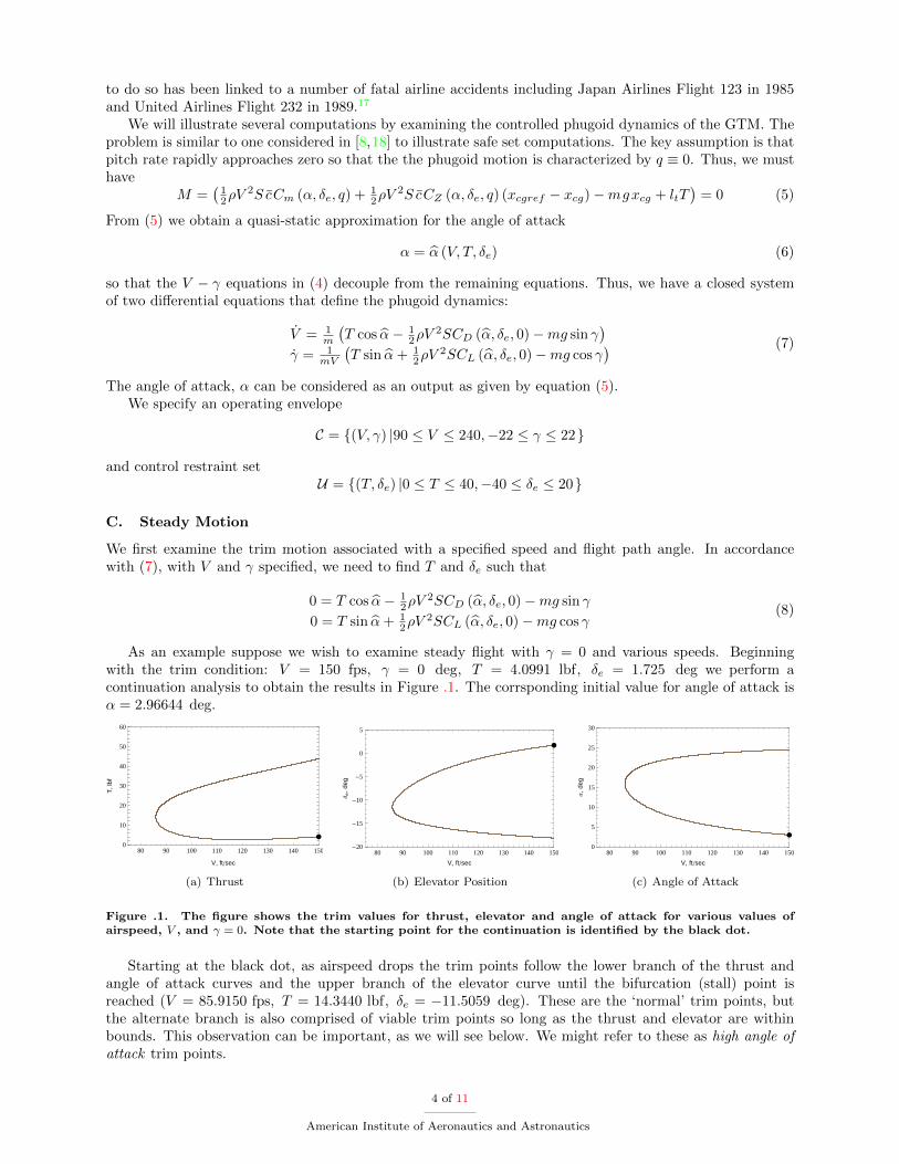
As an example suppose we wish to examine steady flight with γ = 0 and various speeds. Beginningwith the trim condition: V = 150 fps, γ = 0 deg, T = 4.0991 lbf, δe = 1.725 deg we perform acontinuation analysis to obtain the results in Figure .1. The corrsponding initial value for angle of attack isα = 2.96644 deg.

80 90 100 110 120 130 140 1500

10

20

30

40

50

60

V, ftsec

T,l

bf

(a) Thrust

80 90 100 110 120 130 140 150-20

-15

-10

-5

0

5

V, ftsec

∆e,d

eg

(b) Elevator Position

80 90 100 110 120 130 140 1500

5

10

15

20

25

30

V, ftsec

Α,d

eg

(c) Angle of Attack

Figure .1. The figure shows the trim values for thrust, elevator and angle of attack for various values ofairspeed, V , and γ = 0. Note that the starting point for the continuation is identified by the black dot.

Starting at the black dot, as airspeed drops the trim points follow the lower branch of the thrust andangle of attack curves and the upper branch of the elevator curve until the bifurcation (stall) point isreached (V = 85.9150 fps, T = 14.3440 lbf, δe = −11.5059 deg). These are the ‘normal’ trim points, butthe alternate branch is also comprised of viable trim points so long as the thrust and elevator are withinbounds. This observation can be important, as we will see below. We might refer to these as high angle ofattack trim points.

4 of 11

American Institute of Aeronautics and Astronautics

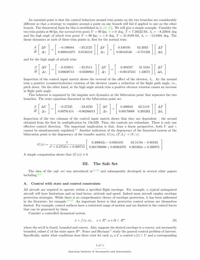
An essential point is that the control behaviors around trim points on the two branches are considerablydifferent so that a strategy to regulate around a point on one branch will fail if applied to one on the otherbranch. The theoretical basis for this is established in [6,19–21]. We will give a simple example. Consider thetwo trim points at 90 fps, the normal trim point, V = 90 fps, γ = 0 deg, T = 7.58222 lbf, δe = −8.22916 degand the high angle of attack trim point, V = 90 fps, γ = 0 deg, T = 21.9189 lbf, δe = −13.8494 deg. Thelinear dynamics at each of these trim points is, first for the normal trim:

d

dt

[∆V

∆γ

]=

[−0.186044 −33.2125

0.008844275 0.0150152

][∆V

∆γ

]+

[0.449195 62.3033

0.00416546 −0.751226

][∆T

∆δe

]

and for the high angle of attack trim:

d

dt

[∆V

∆γ

]=

[−0.310011 −33.2514

0.00638713 −0.0338864

][∆V

∆γ

]+

[0.494357 31.5244

−0.00127241 1.22673

][∆T

∆δe

]

Inspection of the control input matrix shows the reversal of the affect of the elevator, δe. Ay the normaltrim a positive (counterclockwise) rotation of the elevator causes a reduction of the flight path angle, i.e.,pitch down. On the other hand, at the high angle attack trim a positive elevator rotation causes an increasein flight path angle.

This behavior is organized by the singular zero dynamics at the bifurcation point that separates the twobranches. The state equations linearized at the bifurcation point are

d

dt

[∆V

∆γ

]=

[−0.27235 −33.8550

0.00791414 −0.00286013

][∆V

∆γ

]+

[0.400642 62.5119

0.00170008 0.265262

][∆T

∆δe

]

Inspection of the two columns of the control input matrix shows that they are dependent – the secondobtained from the first by multiplication by 156.029. Thus, the controls are redundant. There is only oneeffective control direction. The important implication is that, from a linear perspective, both V and γcannot be simultaneously regulated.22 Another indication of the degeneracy of the linearized system at thebifurcation point is the degeneracy of the transfer matrix, G (s), (T, δe)→ (V, γ):

G (s) =1

s2 + 0.27521s+ 0.268712

[0.400642s− 0.0564101 62.5119s− 8.80163

0.001700086 + 0.00363376 0.265262s+ 0.566973

]

A simple computation shows that |G (s)| ≡ 0.

III. The Safe Set

The idea of the safe set was introduced in18,23 and subsequently developed in several other papersincluding.8,9

A. Control with state and control constraints

All aircraft are required to operate within a specified flight envelope. For example, a typical unimpairedaircraft will have limitations and on load factor, attitude and speed. Indeed most aircraft employ envelopeprotection strategies. While there is no comprehensive theory of envelope protection, it has been addressedin the literature, for example.23–25 An important factor is that protective control actions are themselveslimited. For example, control surfaces have a restricted range of motion and are limited in the control forcesthat can be generated by them.

Consider a controlled dynamical system

x = f (x, u) , x ∈ Rn, u ∈ U ⊂ Rm (9)

where the set U is closed, bounded and convex. Also, suppose the desired envelope is a convex, not necessarilybounded, subset C of the state space Rn. Feuer and Heyman10 study the general control problem of interest.Specifically, under what conditions does there exist for each x0 ∈ C a control u (t) ⊂ U and a corresponding

5 of 11

American Institute of Aeronautics and Astronautics

unique solution x (t;x0, u) that remains in C for all t > 0? While some basic results are provided in [10], thegeneral case is unresolved. Concrete results have subsequently been obtained for special cases, particularlyfor linear dynamics with polyhedral constraint sets.8,9, 18,26–30 In the following paragraphs we apply someof the more recent results.8,9, 18

Suppose that prescribed envelope C is defined by

C = x ∈ Rn |l (x) > 0 (10)

where l : Rn → R is continuous. The boundary of C is the zero level set of l, i.e., ∂C = x ∈ Rn |l (x) = 0.

Definition 3.1 (Controlled-Invariant Set) A set I is a controlled-invariant set over a time interval[t, T ], if for each x (t) ∈ I there exists a control u (τ) ∈ U , τ ∈ [t, T ] such that the solution of (9) emanatingfrom x (t), φ (τ ;x (t) , u (·)), defined on τ ∈ [t, T ] is entirely contained in I.

Definition 3.2 (Safe Set) Given the envelope C as defined in (10), the safe set is defined as the largestcontrolled-invariant set on [t, T ] contained in C, i.e.,

S (t, C) = x ∈ Rn |∃u (τ) ⊂ U ,∀τ ∈ [t, T ] : φ (τ ;x (t) , u (·)) ⊂ C (11)

Several investigators have considered the computation of the safe set, the most compelling of whichinvolve solving the Hamilton-Jacobi equation. We describe one of several variants; this one due to Lygeros.8

The main result in [8] is the following. Suppose V (x, t) is a viscosity (or, weak) solution of the terminalvalue problem

∂V

∂t+ min

0, sup

u∈U

∂V

∂xf (x, u)

= 0, V (x, T ) = l (x) (12)

thenS (t, C) = x ∈ Rn |V (x, t) > 0 (13)

The function V (x, t) is in fact the ‘cost-to-go’ associated with an optimal control problem in which the goalis to choose u (t) so as to maximize the minimum value of l (x (t)). The function V (x, t) inherits some niceproperties from this fact. For instance it is bounded and uniformly continuous. Define the Hamiltonian

H (p, x) = min

0, sup

u∈UpT f (x, u)

(14)

so that (12) can be rewritten:

∂V

∂t+H

(∂V

∂x, x

)= 0, V (x, T ) = l (x) (15)

V (x, t) is the unique, bounded and uniformly continuous solution of (12) or (15). Notice that the controlobtained in computing the Hamiltonian (14) insures that when applied to each state along any trajectoryinitially inside of S the resulting trajectory will remain in S. It follows that this control should be appliedfor states on its boundary to insure that the trajectory does not leave S.

The envelope defined by (10) can be generalized to an envelope with piecewise continuous boundary. Forexample, suppose the envelope is defined by

C = x ∈ Rn |li (x) > 0, i = 1, . . . ,K (16)

Where each of the li (x) are continuous functions. Then we need to solve K problems with

Cj = x ∈ Rn |lj (x) > 0 , j = 1, . . . ,K

to obtain the largest control invariant set in each Cj and then take their intersection. There are many physicalproblems in which the tracking of moving boundaries separating to regions of space are important. So it isnot surprising that the numerical computation of propagating surfaces is a mature field. The most powerfulmethods exploit the connection with the Hamilton-Jacobi equation and associated conservation laws; see thesurvey [31].

6 of 11

American Institute of Aeronautics and Astronautics

100 150 200-0.4

-0.2

0.0

0.2

0.4

V , ftsec

Γ,r

ad

(a) Unimpaired

100 120 140 160 180 200 220 240-0.4

-0.2

0.0

0.2

0.4

V , ftsec

Γ,r

ad

(b) Restricted Elevator

100 120 140 160 180 200 220 240-0.4

-0.2

0.0

0.2

0.4

V , ftsec

Γ,r

ad

(c) Jammed Elevator

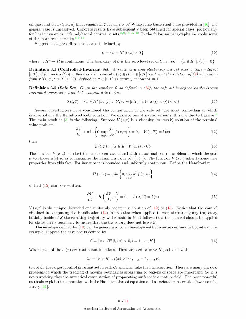
Figure .2. Safe set with various levels of elevator impairment. The figure on the left shows the safe set forthe unimpaired aircraft in which case the elevator position ranges from -40 deg (-0.698 rad) to +20 deg (0.349rad). It is the entire envelope. In the center figure, the elevator motion is restricted in the positive directionto + 3 deg. On the right is the safe set for the aircraft with elevator jammed at 3 deg. The safe set is thesubset of the flight envelope bounded by the black curve.

B. Example: GTM Phugoid Motion

Figure .2 shows the safe set, S for unimpaired and impaired aircraft. As expected, the safe set shrinkswhen the aircraft is impaired. The points in C\S produce trajectories that exit the envelope. With limitedcontrol authority the safe set is reduced in lower left quadrant of (b,c) because at slower speeds, even withthe application of both maximum thrust and elevator deflection, it is not possible to generate enough lift toprevent the aircraft from descending along an unacceptably low flight path angle and leaving the prescribedenvelope C. In the case where the elevator is jammed, the safe set is reduced in the upper right quadrant(c) where the higher speeds cause excessive lift to be generated forcing the aircraft to ascend along a flightpath angle which exceeds the upper bound of C.

IV. Maneuverability

Diminished maneuverability is a central aspect of LOC - whether due to impairment of the aircraft orits entry into an unfavorable flight regime. Maneuverability performance is usually assessed by evaluatingan aircraft’s capability to perform certain basic tasks under a variety of conditions. Such tasks – includingwings level climb and descent, coordinated turns, pull-ups and push-downs – correspond to steady-state orequilibrium motions in an appropriate mathematical setting. The vehicle must be able to transition betweenthese steady motions.

In earlier work6 we introduced an approach to investigating steady motions of aircraft by examiningthe equilibrium point structure of a regulator problem associated with the desired motion. We used acontinuation method to identify bifurcation surfaces in multi-parameter problems and linked bifurcationpoints to structural instability of the zero dynamics. The limits imposed on the ability of a vehicle toperform a maneuver where thereby associated with both the absence of appropriate equilibria for certainparameter values and also with the difficulty to regulate the vehicle when operating near the bifurcation sets.These ideas were further developed and applied in several papers including [7, 32, 33]. A somewhat similarapproach was recently given by Goman et al,34 referred to therein as a constrained trim formulation. Thestability of each equilibrium point is evaluated but no connections are made to control system properties asadvocated in [6].

A. Basic Steady Maneuvers of Rigid Aircraft

For commercial aircraft the most basic and important steady motion are:

1. straight, level, climbing and descending flight,

2. coordinated turns, level, climbing and descending

In [7] we used a continuation method to examine these motions specifically for the GTM. We studiedthe limits imposed on these motions by stall bifurcation points and examined the control system behavioraround these points. Using the results of [6] we argued that regulated flight near stall is difficult because ofthe structurally unstable zero dynamics.

7 of 11

American Institute of Aeronautics and Astronautics

Of course, not all points identified in a continuation computation are feasible trim conditions. Equilibriawith control values outside of the control restraint set need to be excluded. This obvious fact has significantimplications as we will see below.

The idea of aircraft trim is so broadly entrenched that one would assume it requires no further discussion.However, there are subtleties that we need to explore. A general formulation is as follows. Assume the aircraftis described by the state equations in the form of (1) and (2), or (3).

Definition 4.3 (Steady Motion) A steady motion is one for which all 6 velocities are constant, i.e.,u = 0, v = 0, w = 0, (equivalently, V = 0, α = 0, β = 0) and p = 0, q = 0, r = 0. From (2)

F (0,q, µ,u) = 0 (17)

The steady motion requirement, (17), provides six equations to which we add a set of n + m − 6 trimequations:

0 = h (x, u, µ) (18)

Equations (17) and (18) form a set of n + m equations in n + m + k variables. Ordinarily we fix the kparameters, µ and solve for the remaining n+m variables – the state x and the control u.

Definition 4.4 (Trim Point) Given the steady motion equation (17), the trim condition (18), an envelopeC and a control restraint set U , a viable trim point or simply a trim point, with respect to the fixed parameterµ is a pair (x, u) that satisfies (17) and (18) and also x ∈ C, u ∈ U . The set of viable trim points is calledthe trim set, T .

The important point is that for a prescribed trim condition (18) there are often multiple viable trimpoints. The general study of the trim point structure as a function of the parameters is a problem of staticbifurcation analysis.6,7, 33,35,36 When k = 1 this can be carried out using a continuation method. Let usconsider two examples of the trim condition for the six degree of freedom model described in Section II. Inthis case we have four controls. First consider straight wings-level flight:

1. speed, V = V ∗

2. constant roll, pitch and heading, φ = 0, θ = 0, ψ = 0

3. roll angle, φ = 0

4. flight path angle, sin γ∗ + cos θ (cosβ cosφ sinα+ sinβ sinφ)− cosα cosβ sin θ = 0

Now, consider a coordinated turn. In this case the aircraft rotates at constant angular velocity, ω∗ aboutthe inertial z-axis. Thus the attitude of the aircraft varies periodically with time.

1. speed, V = V ∗

2. coordinate turn condition, pV cosβ sinα− rV cosβ cosα+ g cos θ sinφ = 0

3. angular velocity, p = −ω∗ sin θ, q = ω∗ cos θ sinφ, r = ω∗ cos θ cosφ

4. flight path angle, sin γ∗ + cos θ (cosβ cosφ sinα+ sinβ sinφ)− cosα cosβ sin θ = 0

We generally view the set of trim viable trim points, T , in the state-control-parameter space, X×U×M ⊂Rn+m+k. Typically, the set of trim conditions is a smooth k-dimensional submanifold of this n + m + k-dimensional manifold. It is common practice in bifurcation theory to project T onto the parameter spaceM. The result is the bifurcation picture. The folds of T project onto M as k − 1-dimensional submanifoldsof M. So they partition M into k-dimensional disjoint regions. Each region contains a distinct number oftrim points.

If we project T onto the n-dimensional state space X the result is a k-dimensional subset (possibly quitecomplex) of X that is also partitioned into subsets by the folds of T . Again each subset is associated witha distinct number of trim points. The significance of this is that the process identifies the possible trimstates and identifies the number of trim points associated with each such state. This is important for controlanalysts and designers concerned with state to state transitions.

8 of 11

American Institute of Aeronautics and Astronautics

B. Example: GTM Phugoid Model

We would expect that since the unimpaired aircraft has two independent controls and only two states thatevery point in the envelope could be made an equilibrium point by proper choice of control. The only issueis that the controls are bounded. However, the situation is more complicated than that. In fact, in thiscase there is one and sometimes two admissible control pairs for which each point in the state space can bemade an equilibrium point. Even so, maneuverability can be problematic. To understand the problem, firstcompute the values of the controls (T, δe) required to force an arbitrary point (V, γ) to be an equilibriumpoint.

80 90 100 110 120 130 140 1500

10

20

30

40

50

60

V, ftsec

T,l

bf Γ=-22.3Γ=-11.5Γ=-5.7Γ=0Γ=5.7Γ=11.5Γ=22.3

(a) Thrust

80 90 100 110 120 130 140 150-20

-15

-10

-5

0

5

V, ftsec

∆e,d

eg

Γ=-22.3Γ=-11.5Γ=-5.7Γ=0Γ=5.7Γ=11.5Γ=22.3

(b) Elevator

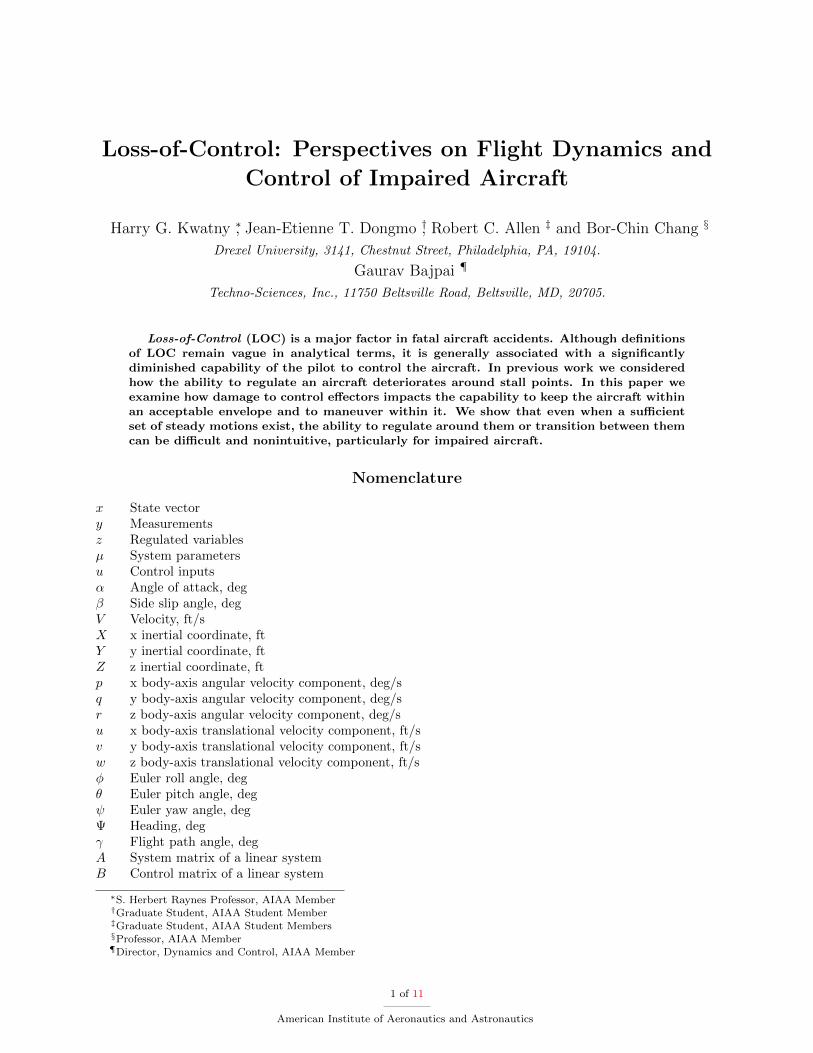
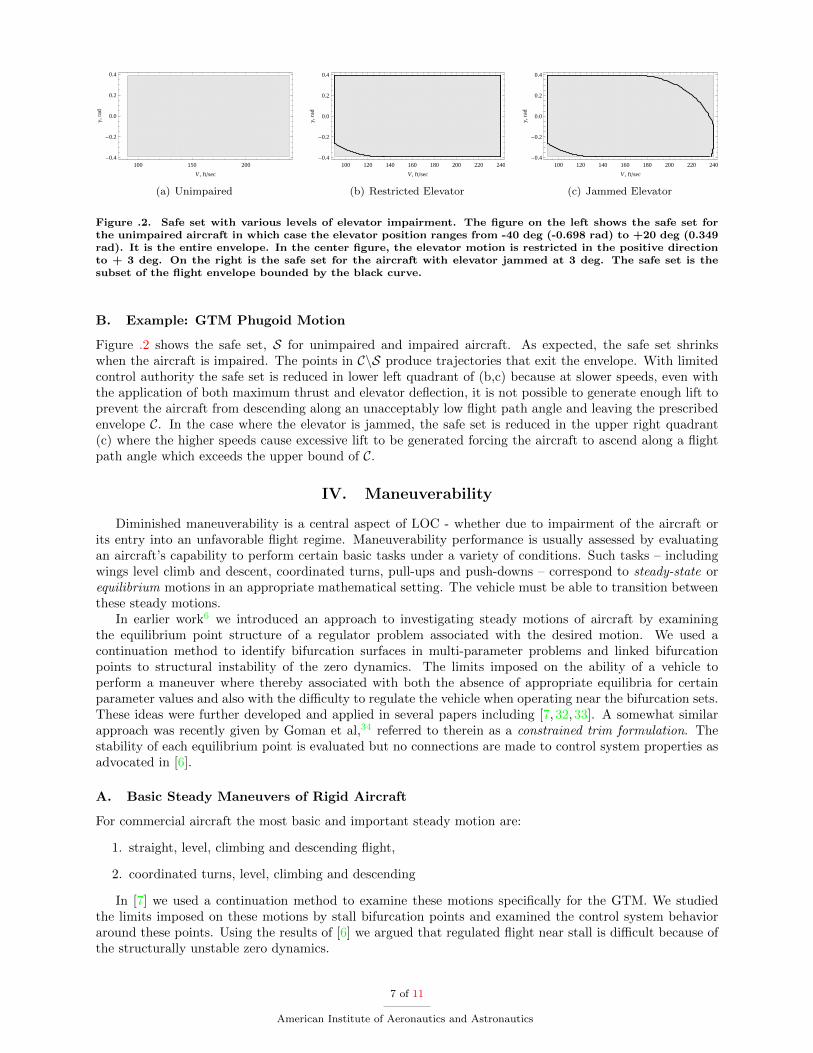
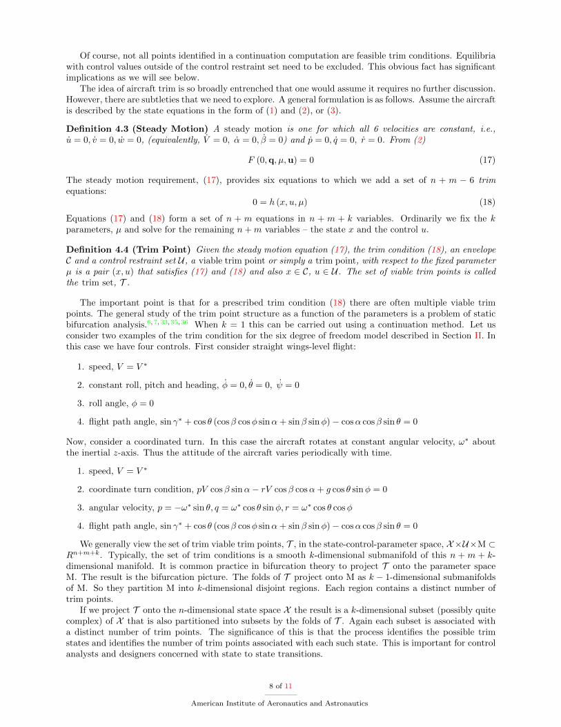
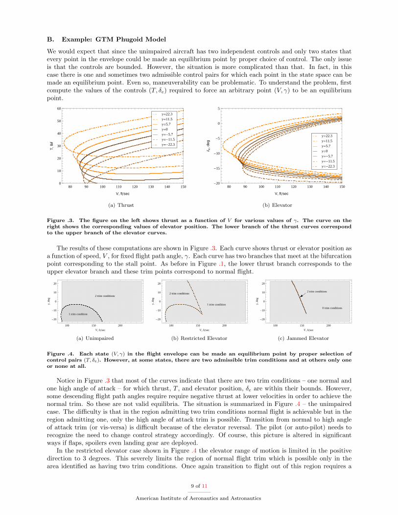
Figure .3. The figure on the left shows thrust as a function of V for various values of γ. The curve on theright shows the corresponding values of elevator position. The lower branch of the thrust curves correspondto the upper branch of the elevator curves.

The results of these computations are shown in Figure .3. Each curve shows thrust or elevator position asa function of speed, V , for fixed flight path angle, γ. Each curve has two branches that meet at the bifurcationpoint corresponding to the stall point. As before in Figure .1, the lower thrust branch corresponds to theupper elevator branch and these trim points correspond to normal flight.

2 trim conditions

1 trim condition

100 150 200

-20

-10

0

10

20

V , ftsec

Γ,d

eg

(a) Unimpaired

2 trim conditions

1 trim condition

100 150 200

-20

-10

0

10

20

V , ftsec

Γ,d

eg

(b) Restricted Elevator

0 trim conditions

2 trim conditions

100 150 200

-20

-10

0

10

20

V , ftsec

Γ,d

eg

(c) Jammed Elevator

Figure .4. Each state (V, γ) in the flight envelope can be made an equilibrium point by proper selection ofcontrol pairs (T, δe). However, at some states, there are two admissible trim conditions and at others only oneor none at all.

Notice in Figure .3 that most of the curves indicate that there are two trim conditions – one normal andone high angle of attack – for which thrust, T , and elevator position, δe are within their bounds. However,some descending flight path angles require require negative thrust at lower velocities in order to achieve thenormal trim. So these are not valid equilibria. The situation is summarized in Figure .4 – the unimpairedcase. The difficulty is that in the region admitting two trim conditions normal flight is achievable but in theregion admitting one, only the high angle of attack trim is possible. Transition from normal to high angleof attack trim (or vis-versa) is difficult because of the elevator reversal. The pilot (or auto-pilot) needs torecognize the need to change control strategy accordingly. Of course, this picture is altered in significantways if flaps, spoilers even landing gear are deployed.

In the restricted elevator case shown in Figure .4 the elevator range of motion is limited in the positivedirection to 3 degrees. This severely limits the region of normal flight trim which is possible only in thearea identified as having two trim conditions. Once again transition to flight out of this region requires a

9 of 11

American Institute of Aeronautics and Astronautics

change to high angle of attack trim, which involves a significant increase in throttle, a decrease in elevatorand results in a reversal in the effect of elevator.

V. Conclusions

In this paper we continue an examination of mechanisms of LOC. The main focus here is on the impactof control constraints, including those induced by actuator impairment, on the maneuverability within theadmissible flight envelope. We used the phugoid dynamics of the GTM to provide a simple illustration ofsafe set computation and the effect of failures on the safe set. We examined maneuverability by identifyingsteady motions within the safe set and illustrated how the set of trim points can change structure whenactuator impairment occurs.

An aircraft is trimmed to achieve a desired steady motion such as straight and level flight or a coordinatedturn. The specification expressed as a set of algebraic equations is called the trim condition. The specificationis generally made in terms of a set of k parameters. For example, in the case of straight and level flight wemight consider speed and flight path angle to be parameters (k = 2). In the case of a coordinated turn wemight consider, speed, flight path angle and angular velocity (equivalently, turn radius), so k = 3. To achievethe specified trim we need to identify the required controls and the associated state. These are obtained assolutions to the trim equations. For each trim condition and fixed parameters there may be zero, one, ormore corresponding pairs of control and state values. We call these the trim points corresponding to thetrim condition. For a trim point to be viable, the control must be within the allowable control set and thestate must be within the safe set. The trim condition is viable only if it is associated with at least one viabletrim point.

The trim equations depend on the values specified for the k trim parameters. This is a classic staticbifurcation problem. Typically, the solution set is a smooth k-dimensional submanifold of an n + m + k-dimensional space of states, controls and parameters. The solution manifold is divided into components byco-dimension one bifurcation sets. In general, we can associate each trim point with a specific component ofthe solution manifold. In the phugoid example, the two dimensional solution set has two components. Weidentified these as normal and high angle of attack. Not all of these are viable.

We considered transitions between trim points and showed that transition from one trim condition couldrequire moving from one trim point to another which belongs to a different component. In this case, thecontrol properties at the two trim conditions would be quite different, thereby requiring a change in strategyfor regulating around the new trim condition.

References

1Russell, P. and Pardee, J., “Final Report: JSAT Loss of Control: Results and Analysis,” Tech. rep., Federal AviationAdministration: Commercial Airline Safety Team, 2000.

2Ranter, H., “Airliner Accident Statistics 2006,” Tech. rep., Aviation Safety Network, 2007.3Anonymous, “Statistical Summary of Commercial Jet Airplane Accidents - Worldwide Operations 1959-2007,” Tech. rep.,

Boeing Corporation, 2008.4Lambregts, A. A., Nesemeier, G., Wilborn, J. E., and Newman, R. E., “Airplane Upsets: Old Problem, New Issues,”

AIAA Modeling and Simulation Technologies Conference and Exhibit , AIAA, Honolulu, Hawaii, 2008.5Wilborn, J. E. and Foster, J. V., “Defining Commercial Aircraft Loss-of-Control: a Quantitative Approach,” AIAA

Atmospheric Flight mechanics Conference and Exhibit , AIAA, Providence, Rhode Island, 16-19 August 2004.6Kwatny, H. G., Bennett, W. H., and Berg, J. M., “Regulation of Relaxed Stability Aircraft,” IEEE Transactions on

Automatic Control , Vol. AC-36, No. 11, 1991, pp. 1325–1323.7Kwatny, H. G., Dongmo, J.-E. T., Chang, B. C., Bajpai, G., Yasar, M., and Belcastro, C., “Aircraft Accident Prevention:

Loss-of-Control Analysis,” AIAA Guidance, Navigation and Control Conference, Chicago, 10-13 August 2009.8Lygeros, J., “On Reachability and Minimum Cost Optimal Control,” Automatica, Vol. 40, 2004, pp. 917–927.9Oishi, M., Mitchell, I. M., Tomlin, C., and Saint-Pierre, P., “Computing Viable Sets and Reachable Sets to Design

Feedback Linearizing Control Laws Under Saturation,” 45th IEEE Conference on Decision and Control , IEEE, San Diego,2006, pp. 3801–3807.

10Feuer, A. and Heymann, M., “Ω-Invariance in Control Systems wiyh Bounded Controls,” Journal of mathematicalAnalysis and Applications, Vol. 53, 1976, pp. 26–276.

11Jordan, T., Langford, W., Belcastro, C., Foster, J., Shah, G., Howland, G., and Kidd, R., “Development of a DynamicallyScaled Generic Transport Model Testbed for Flight Research Experiments,” AUVSI Unmanned Unlimited , Arlington, VA, 2004.

12Kwatny, H. G. and Blankenship, G. L., Nonlinear Control and Analytical Mechanics: a computational approach, ControlEngineering, Birkhauser, Boston, 2000.

10 of 11

American Institute of Aeronautics and Astronautics

13Murch, A. M. and Foster, J. V., “Recent NASA Research on Aerodynamic Modeling of Post-Stall and Spin Dynamics ofLarge Transport Aircraft,” 8-11 January 2007.

14Morelli, E. A., “Global Nonlinear Aerodynamic Modeling Using Multivariate Orthogonal Functions,” Journal of Aircraft ,Vol. 32, No. 2, 1995, pp. 270–277.

15Morelli, E. A. and DeLoach, R., “Wind Tunnel Database Development using Modern Experiment Design and MultivariateOrthogonal Functions,” 41st AIAA Aerospace Sciences Meeting and Exhibit , AIAA Paper 2003-0653, Reno, NV, January 2003.

16Lanchester, F. W., Aerodonetics, Constable and Company, London, 1908.17Anonymous, “Aircraft Accident Report – United Airlines Flight 232,” Tech. Rep. NTSB/AAR-90/06, National Trans-

portation Safety Board, 1990.18Lygeros, J., Tomlin, C., and Sastry, S., “Controllers for reachability specifications for hybrid systems,” Automatica,

Vol. 35, No. 3, 1999, pp. 349–370.19Berg, J. and Kwatny, H. G., “An Upper Bound on the Structurally Stable Regulation of a Parameterized Family of

Nonlinear Control Systems,” Systems and Control Letters, Vol. 23, 1994, pp. 85–95.20Berg, J. and Kwatny, H. G., “A Canonical Parameterization of the Kronecker Form of a Matrix Pencil,” Automatica,

Vol. 31, No. 5, 1995, pp. 669–680.21Berg, J. M. and Kwatny, H. G., “Unfolding the Zero Structure of a Linear Control System,” Linear Algebra and its

Applications, Vol. 235, 1997, pp. 19–39.22Wonham, W. M., Linear Multivariable Control: A Geometric Approach, Springer-Verlag, NY, 3rd ed., 1985.23Tomlin, C., Lygeros, J., and Sastry, S., “Aerodynamic Envelope Protection using Hybrid Control,” American Control

Conference, Philadelphia, 1998, pp. 1793–1796.24Unnikrishnan, S. and Prasad, J. V. R., “Carefree Handling Using Reactionary Envelope Protection Method,” AIAA

Guidance, Navigation and Control Conference and Exhibit , Keystone, CO, 21-24 August 2006.25Well, K. H., “Aircraft Control Laws for Envelope Protection,” AIAA Guidance, Navigation and Control Conference,

Keystone, Colorado, 21-24 August 2006.26Glover, J. D. and Schweppe, F. C., “Control of Linear Systems with Set Constrained Disturbances,” IEEE Transactions

on Automatic Control , Vol. 16, No. 5, 1971, pp. 411–423.27Blanchini, F., “Feedback Control for Linear Time-Invariant Systems with State and Control Bounds in the Presence of

Uncertainty,” IEEE Transactions on Automatic Control , Vol. 35, No. 11, 1990, pp. 1231 – 1234.28Bitsoris, G. and Gravalou, E., “Comparison Principle, Positive Invariance and constrained regulation of Nonlinear Sys-

tems,” Automatica, Vol. 31, No. 2, 1995, pp. 217–222.29Bitsoris, G. and Vassilaki, M., “Constrained Regulation of Linear Systems,” Automatica, Vol. 31, No. 2, 1995, pp. 223–

227.30ten Dam, A. A. and Nieuwenhuis, J. W., “A Linear programming Algorithm for Invariant Polyhedral Sets of Discrete-Time

Linear Systems,” Systems and control Letters, Vol. 25, 1995, pp. 337–341.31Sethian, J. A., “Evolution, Implementation, and Application of Level Set and Fast Marching Methods for Advancing

Fronts,” Journal of Computational Physics, Vol. 169, 2001, pp. 503–555.32Thomas, S., Kwatny, H. G., and Chang, B. C., “Nonlinear Reconfiguration for Asymmetric Failures in a Six Degree-of-

Freedom F-16,” American Control Conference, IEEE, Boston, MA, June/July 2004, pp. 1823–1829.33Thomas, S., Kwatny, H. G., and Chang, B. C., “Bifurcation Analysis of Flight Control Systems,” IFAC World Congress,

Prague, 2005.34Goman, M. G., Khramtsovsky, A. V., and Kolesnikov, E. N., “Evaluation of Aircraft Performance and Maneuverability by

Computation of Attaiable Equilibrium Sets,” Journal of Guidance, Control and Dynamics, Vol. 31, No. 2, 2008, pp. 329–339.35Thomas, S., Reconfiguration and bifurcation in flight controls, Ph.D. thesis, Drexel University, Philadelphia, December

2004. [Online] http://dspace.library.drexel.edu/handle/1860/385.36Bajpai, G., Beytin, A., Thomas, S., Yasar, M., Kwatny, H. G., and Chang, B. C., “Nonlinear Modeling and Analysis

Software for Control Upset Prevention and Recovery of Aircraft,” AIAA Guidance, Navigation and Control Conference, AIAA,Honolulu, Hawaii, 18-21 August 2008.

11 of 11

American Institute of Aeronautics and Astronautics