LOSSCALCTM: MODEL FOR PREDICTING LOSS GIVEN DEFAULT (LGD)

MODELINGMETHODOLOGY

This report describes and documents LossCalc, Moody's model for predicting loss given default(LGD): the equivalent of (1 - recovery rate. LGD is of natural interest to investors and lenderswishing to estimate future credit losses. LossCalc is a robust and validated model of United StatesLGD for bonds, loans, and preferred stock. It produces estimates of LGD for defaults occurringimmediately and for defaults occurring in one year. These two point-in-time estimates can be usedto predict LGD over holding periods.

LossCalc is a statistical model that incorporates information on instrument, firm, industry, andeconomy to predict LGD. It improves upon traditional reliance on historical recovery averages.The model is based on over 1,800 observations of U.S. recovery values of defaulted loans, bonds,and preferred stock covering the last two decades. This dataset includes over 900 defaulted publicand private firms in all industries.

We believe LossCalc is a meaningful addition to the practice of credit risk management and a stepforward in answering the call for rigor that the BIS has outlined in their recently proposed BaselCapital Accord.

FIGURE 1

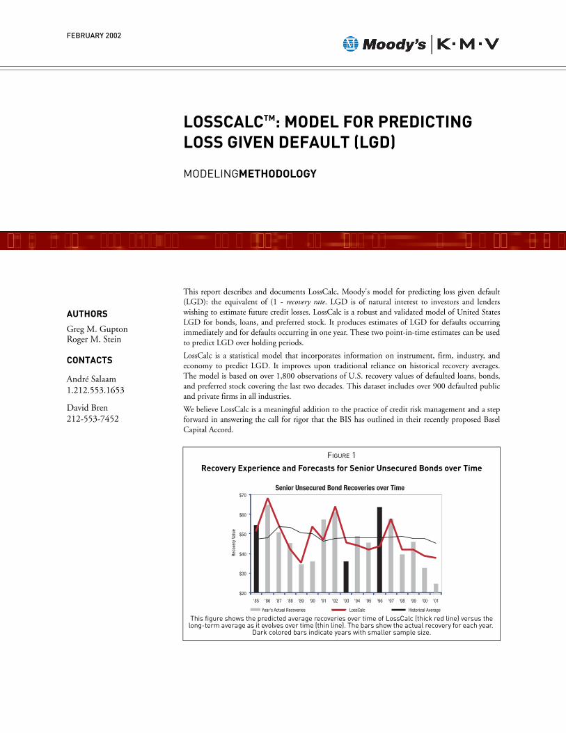
Recovery Experience and Forecasts for Senior Unsecured Bonds over Time

This figure shows the predicted average recoveries over time of LossCalc (thick red line) versus the long-term average as it evolves over time (thin line). The bars show the actual recovery for each year.

Dark colored bars indicate years with smaller sample size.

Senior Unsecured Bond Recoveries over Time

$20

$30

$40

$50

$60

$70

'85 '86 '87 '88 '89 '90 '91 '92 '93 '94 '95 '96 '97 '98 '99 '00 '01

Reco

very

Val

ue

Year's Actual Recoveries LossCalc Historical Average

FEBRUARY 2002

AUTHORS

Greg M. GuptonRoger M. Stein

CONTACTS

André Salaam1.212.553.1653

David Bren212-553-7452

© 2003 Moody’s KMV Company. All rights reserved. Credit Monitor®, EDFCalc®, Private Firm Model®, KMV®, CreditEdge, Portfolio Manager,Portfolio Preprocessor, GCorr, DealAnalyzer, CreditMark, the KMV logo, Moody's RiskCalc, Moody's Financial Analyst, Moody's Risk Advisor,LossCalc, Expected Default Frequency, and EDF are trademarks of MIS Quality Management Corp.

Published by:

Moody’s KMV Company

To Learn More

Please contact your Moody’s KMV client representative, visit us online at www.moodyskmv.com, contact Moody’s KMV via e-mail at info@mkmv.com,or call us at:

NORTH AND SOUTH AMERICA, NEW ZEALAND AND AUSTRALIA, CALL:

1 866 321 MKMV (6568) or 415 296 9669

EUROPE, THE MIDDLE EAST, AFRICA AND INDIA, CALL:

44 20 7778 7400

FROM ASIA CALL:

813 3218 1160

We have organized the remainder of this report as follows:

Section 1, Loss Given Default: discusses the importance and difficulty of estimating loss given default (LGD), which is of naturalinterest to investors and lenders. Its estimation is as important as the probability of default in predicating credit losses.

Section 2, The LossCalc Model: describes the LossCalc LGD model and summarizes the factors of the model, the modeling frame-work, model validation results, and the dataset. We discuss each of these topics in more detail in subsequent sections.

Section 3, Factors: describes the nine predictive factors that drive the estimate of LGD in the LossCalc model.

Section 4, Framework: describes the modeling approach we used to develop LossCalc.

Section 5, Validation and Testing: documents the performance of the model in out-of-sample, out-of-time testing, which we findto be superior to traditional LGD estimation methods.

Section 6, The Dataset: describes the data used to develop the model and gives details of the dataset which contains over 1,800observations of U.S. recovery values of defaulted loans, bonds, and preferred stock covering the last two decades.

Highlights1. We describe Moody's LossCalcTM, a predictive statistical model of loss given default (LGD), the factors in the model, the

modeling approach, and the accuracy of the model.2. We find that LossCalc performs better at predicting LGD than traditional historical average methods. LossCalc:

• exhibits lower prediction error and higher correlation with actual losses;• is more powerful at predicting low recoveries; and• produces narrower confidence bounds.

3. LossCalc produces estimates of LGD for defaults occurring immediately and for defaults occurring in one year.4. Moody's has based LossCalc on over 1,800 observations of U.S. recovery values of defaulted loans, bonds, and preferred stock

covering the last two decades. This dataset includes over 900 defaulted public and private firms in all industries.

AcknowledgementsThe authors would like to thank the numerous individuals who contributed to the ideas, modeling, validation, testing and ultimatelywriting of this document. Eduardo Ibarra provided significant research support for this project. We also thank the following people fortheir comments: Richard Cantor, Lea V. Carty, Jerome Fons, Daniel Gates, and Douglas Lucas, all of Moody's; Dr. Philipp J.Schönbucher, of Bonn University; and Prof. Jeffrey S. Simonoff, of New York University; and Phil Escott, of Oliver, Wyman &Company.We also received invaluable feedback from Moody's Academic Advisory and Research Committee during the presentation of thismodel and in discussions afterwards, particularly Darrell Duffie, of Stanford University; William Perraudin, of Birkbeck College; andJohn Hull, of the University of Toronto. Moody's Quantitative Tools Standing Committee also provided helpful suggestions thatgreatly improved the model.

LOSSCALCTM: MODEL FOR PREDICTING LOSS GIVEN DEFAULT (LGD) 3

TABLE OF CONTENTS

1. LOSS GIVEN DEFAULT 42. THE LOSSCALC LGD MODEL 5

2.1 Overview 52.2 Time Horizon 62.3 Factors 62.4 Framework 62.5 Validation 72.6 The Dataset 7

3. FACTORS 73.1 Definition Of Loss Given Default 73.2 Factor Descriptions 8

3.2.1 Debt Type and Seniority 93.2.2 Firm Specific Capital Structure: Leverage 103.2.3 Industry 103.2.4 Macro Economic 10

3.2.4.1 One-Year RiskCalc Probability of Default 113.2.4.2 Moody's Bankrupt Bond Index 113.2.4.3 Trailing 12-month Speculative Grade Average Default Rates 113.2.4.4 Changes in Index of Leading Economic Indicators 11

4. FRAMEWORK 124.1 Establishing A Dependent Variable 124.2 Transformation And Mini-modeling 14

4.2.1 The Index of Macro Changes 144.2.2 Factor Inclusion by Seniority Class and Industry 14

4.3 Modeling And Mapping: Explanation To Prediction 144.4 Confidence Interval Estimation 14

5. VALIDATION AND TESTING 155.1 Alternative Recovery Models Used As Benchmarks 15

5.1.1 Table of Historical Averages 155.1.2 The Historical Mean Recovery Rate 16

5.2 The Losscalc Validation Tests 165.2.1 Prediction Error Rates 165.2.2 Correlation with Actual Recoveries 185.2.3 Relative Performance for Specific Debt Types 195.2.4 Prediction of Larger Than Expected Losses 195.2.5 Reliability and Width of Confidence Intervals 21

6. THE DATASET 226.1 Historical Time Period Analyzed 226.2 Scope Of Geographic Coverage And Legal Domain 236.3 Scope Of Firm Types And Instrument Categories 23

7. CONCLUSION 24APPENDIX A: BETA TRANSFORMATION TO NORMALIZE LOSS DATA 25APPENDIX B: AN OVERVIEW OF THE VALIDATION APPROACH 26

B.1. Controlling For "Over Fitting" Risk: Walk-forward Testing 26B.2. Resampling 27

GLOSSARY OF TERMS 28

4

1. LOSS GIVEN DEFAULTLoss Given Default, the equivalent of (1 - recovery rate is of natural interest to investors and lenders who wish to estimatepotential credit losses. However, it is inherently difficult to predict what the value or cash flows of an obligation might beif it became defaulted. When a loan is made or a security purchased, the holder does not normally think it likely that theobligor will default. Yet, to predict LGD, the creditor must imagine the circumstances that would cause default and thecondition of the obligor after such default.

The practicalities of the U.S. bankruptcy process make it difficult to predict how the value of a bankrupt firm will beapportioned among its creditors. In U.S. bankruptcy legislation, the guiding principal for allocating a firm's liquidationvalue amongst its creditors is the seniority hierarchy or "classes" of claims applied using the Absolute Priority Rule In itsstrictest interpretation, each class has a relative ranking. Funds available for distributions are paid first to the highest-rankingclass until the firm's obligations to it are fully satisfied. Only then would the next highest-ranking class start to be paid.

This strict interpretation of priority is almost never fully adhered to (see for example Longhofer & Carlstrom [1995]).Indeed, bankruptcy procedures include the drafting of a "plan" that can only proceed speedilyupon the approval ofmultiple levels of claimants. Thus, to gain control of the company quickly, and stop any further deterioration of assetvalues from occurring, there is incentive for senior claimants to make concessions to junior claimants. In the end, recoveryrates have a lot to do with not only the assets of the bankrupt firm and the seniority of a petitioner's claim, but also therelative strength of negotiating positions.

LGD is as important as the probability of default in estimating potential credit losses. We can see this immediately byconsidering the formula for credit loss:

Potential Credit Loss = Probability of Default x Loss Given Default

A proportional error in either the probability of default or LGD affects potential credit losses identically. Yet, much moreresource and effort is employed to estimate probability of default. Many different modeling techniques are applied todefault probability; from statistical methods based on accounting data to structural (Merton) models to hybrids such asMoody's RiskCalc™.

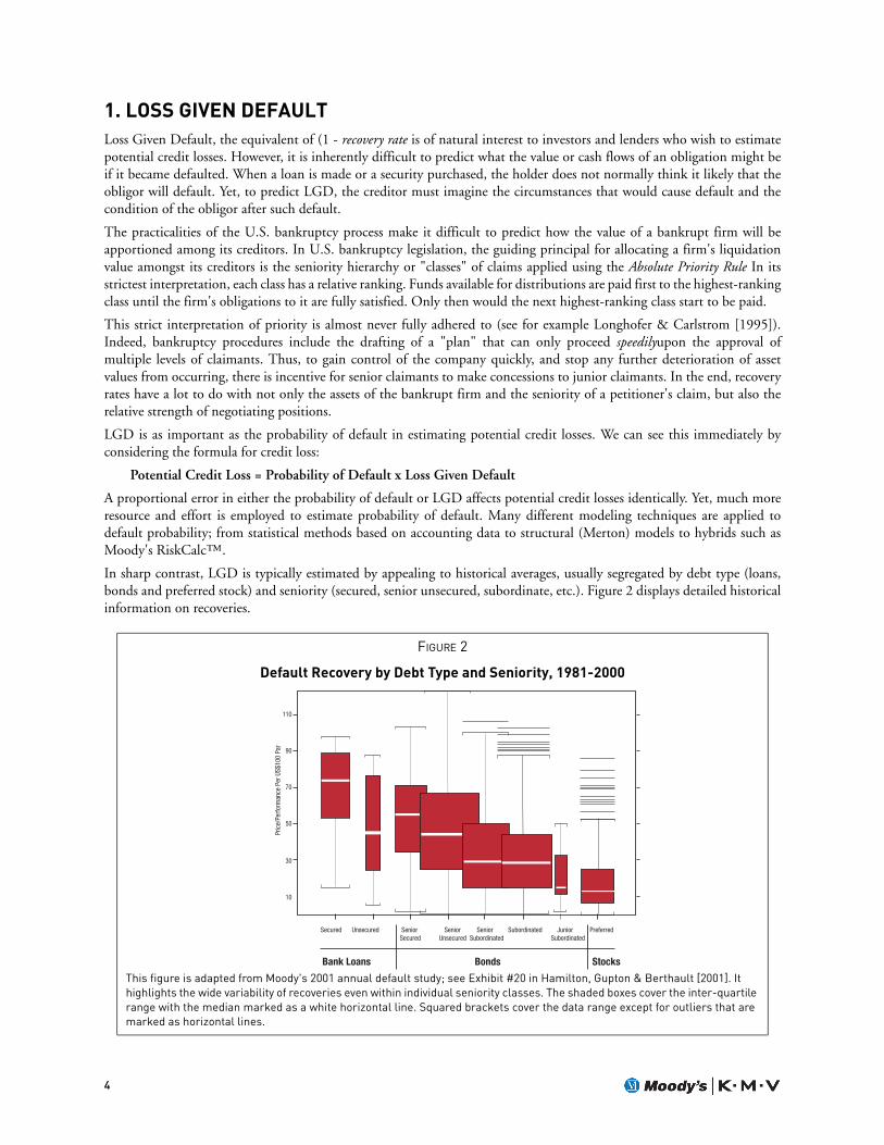
In sharp contrast, LGD is typically estimated by appealing to historical averages, usually segregated by debt type (loans,bonds and preferred stock) and seniority (secured, senior unsecured, subordinate, etc.). Figure 2 displays detailed historicalinformation on recoveries.

FIGURE 2

Default Recovery by Debt Type and Seniority, 1981-2000

This figure is adapted from Moody's 2001 annual default study; see Exhibit #20 in Hamilton, Gupton & Berthault [2001]. It highlights the wide variability of recoveries even within individual seniority classes. The shaded boxes cover the inter-quartile range with the median marked as a white horizontal line. Squared brackets cover the data range except for outliers that are marked as horizontal lines.

Secured Unsecured Senior Senior Senior Subordinated Junior Preferred Secured Unsecured Subordinated Subordinated

Bank Loans Bonds Stocks

110

90

70

50

30

10

Pric

e/Pe

rform

ance

Per

US$

100

Par

LOSSCALCTM: MODEL FOR PREDICTING LOSS GIVEN DEFAULT (LGD) 5

The extreme range of the historical data should make one wonder about its use. For example, suppose one used themedian (32%) to estimate recovery on a senior subordinated bond. The median absolute error of that estimate (out ofsample) is over 22%. Compared to the 32% median, the range of the error is almost 70% (=22/32) of the estimate. Thesame percentage absolute error in default probabilities for a senior subordinated bond with a senior implied rating of Baaand a 10-year maturity would imply a historical default rate somewhere in the very wide range of Aa-to-almost-Ba!1

Recently, regulatory bodies have focused more closely on LGD analysis. The proposed New Basel Capital Accord (Basel,2001) addresses the issue explicitly:

Where there is no explicit maturity dimension in the foundation approach,corporate exposures will receive a risk weight that depends on theprobability of default (PD) and loss given default (LGD).

(Basel, § 173)

Banks would have the option of using conservative pre-defined LGD measures under the so-called foundation approach,but if they wish to qualify for the advanced approach:

…A bank must estimate an LGD for each of its internal LGD grades…Eachestimate of LGD must be grounded in historical experience and empiricalevidence. At the same time, these estimates must be forwardlooking…LGD estimates that are based purely on subjective or judgmentalconsideration and not grounded in historical experience and data will berejected by supervisors.

(Basel, § 336 & 337)

We believe that LossCalc is a meaningful addition to the practice of credit risk management and a step forward inanswering the call for rigor that the BIS has outlined in their recently proposed Basel Capital Accord.

2. THE LOSSCALC LGD MODEL

2.1 OverviewLossCalc is a robust and validated model of United States LGD for bonds, loans, and preferred stock. It producesestimates of LGD for defaults occurring immediately and for defaults occurring in one year.

The issue of prediction horizon has received little attention in previous recovery research, perhaps due to the static natureofa typical table of long-term historical averages. Applications of historical average tables typically use the same estimate ofrecovery irrespective of the horizon over which default might occur. This means that important considerations are ignoredsuch as the point in the credit cycle or the sensitivity of a borrower to the economic environment. It is the nature ofhistorical average LGD methods to be updated infrequently. In addition, new data will have a relatively small impact onlonger-term averages.

In contrast, LossCalc is dynamicand able to give a more exact specification of LGD horizon that incorporates cyclic andfirm specific effects. LossCalc's immediate and one-year horizon forecasts would naturally fit different investor and riskmanagement applications.

LossCalc incorporates information on instrument, firm, industry, and economy to predict LGD. It improves upontraditional reliance on historical recovery averages. We have developed the model on over 1,800 observations of U.S.recovery values of defaulted loans, bonds, and preferred stock covering the last two decades. This dataset includes over 900defaulted public and private firms in all industries.

1. The 10-year default rate on a Baa is just under 8% (here we round from the historical 7.92% rate). Using the mean absolute deviation as a measure of error, we observed about a 22/32 » 70% error rate on the LGD estimate. The equivalent 70% difference in default probability would imply:

a lower bound of: 8% - 0.7*8% = 2.4%; and an upper bound of: 8% + 0.7*8% =13.6%.

The Aa 10-year default rate is 3.1%, which is still higher than our lower bound, so the upper bound would be equivalent to at least a Aa-rating. The upper bound is below the 10-year Baa default rate of 7.92% and above the 10-year Ba default rate of 19.05%. Refer to Exhibits #30 and #31 in Keenan, Hamilton & Berthault [2000] for the default rates. This is a stylized example.

6

2.2 Time HorizonThe time horizon of LGD projections is an important aspect of credit risk that has unfortunately been absent from riskmanagement practices. The valuation of a defaulted debt is far from static and should change with different forecasthorizons. This is true for the valuation of any asset. Investors and lenders should match the tenor of the LGD projectionto their exposure horizon.

Nevertheless, the prevailing practice is to treat LGD as static over the holding period. LossCalc projects LGD for two pointsin time: immediate and at one year. Assuming no knowledge of the individual obligor, the average time of a possible defaultwould be about half way into the exposure period. This means that LossCalc's immediate prediction of LGD should beapplied to exposures maturing in less than one year and with an average time to default of less than six-months. Theimmediate version can also be used for debts that are already in default, particularly if market prices are not available.

The one-year version of LossCalc projects LGD for default in one year. Therefore, it is ideal for two-year exposures thathave an average time to default of one year. The one-year LossCalc LGD is also the best prediction for exposures one yearand greater. The user should note changes in exposure amount when determining which LGD projection to use.

2.3 FactorsAs a proxy for the ultimate recovery on a defaulted instrument, we use the market value of defaulted debt one-monthafter default.

LossCalc uses nine explanatory factors to predict LGD. We have summarized these nine factors into four broad groups asshown below:

• debt-type: (i.e., loan, bond, and preferred stock) and seniority grade (e.g., secured, senior unsecured,subordinate, etc.);

• firm specific capital structure: leverage and seniority standing;

• industry: moving average of industry recoveries; banking industry indicator;

• macroeconomic: one-year median RiscCalc default probability; Moody's Bankrupt Bond Index; trailing 12-month speculative grade default rate; changes in the index of Leading Economic Indicators.

These factors have little intercorrelation, each is statistically significant, and together they make a more accurate predictionof LGD.

2.4 FrameworkWe have based LossCalc on a methodological framework similar to that used in Moody's RiskCalc probability of defaultmodels. The broad steps in this framework are transformation, modeling, and mapping.

Transformation: We transform raw data into "mini-models." For example, we have found it useful to transform certainmacro-economic variables into composite indices, rather than use the pure levels. As another example, we find it useful touse average historical LGD by debt type and seniority.

Modeling: Once we have transformed individual factors and converted them into mini-models, we aggregate these usingregression techniques.

Mapping: We statistically map the model output to historical LGD.

Each of the three steps to this process relies on the application of standard statistical techniques. We outline the details ofthese in Section 4.

LOSSCALCTM: MODEL FOR PREDICTING LOSS GIVEN DEFAULT (LGD) 7

2.5 ValidationWe find that LossCalc is a better predictor of LGD than the traditional methodologies of historical averages segmented bydebt type and seniority. By "better," we mean that:

• LossCalc estimates have significantly lower error.• LossCalc makes far fewer large errors. A reduction in very large errors is the principal driver of the overall

reduction in error. For example, LossCalc has about 50% fewer errors larger than 30% of par value.

• LossCalc estimates have significantly more correlation with actual outcomes. This means they have better trackingof high and low recoveries.

• LossCalc provides better discrimination between instruments of the same type. For example, the model provides amuch better ordering (best to worst recoveries) of bank loans than historical averages.

• Over 10% of the time, the reduction in error rate is greater than 12% of original par value.• LossCalc, on average, has tighter confidence bounds than other approaches so there is more certainty of

recovery prediction.

2.6 The DatasetWe developed the model on over 1,800 observations of U.S. LGD of defaulted loans, bonds, and preferred stock coveringthe last two decades. This dataset includes over 900 defaulted public and private firms in all industries. The issue sizesrange from $680 thousand to $2.0 billion, with a median size of about $100 million. The median firm size (assets atannual report before default) was $660 million, but ranged from $5.0 million to $37.7 billion. Neither debt size nor firmsize appears significantly predictive of recovery rate in this dataset.

3. FACTORSIn this section, we describe the LGD variable and the explanatory factors of the immediate and one-year LossCalc models.The modeling framework is a statistical modeling approach. The central goal is to increase predictive power through theinclusion of multiple factors, each designed to capture specific aspects of LGD determination.

3.1 Definition Of Loss Given DefaultWe define recovery on a defaulted instrument as its market value approximately one-month after default.2 Importantly, weuse security-specific bid-side market quotes.3 These prices are not"matrix" prices, which are broker-created tables specifiedacross maturity, credit grade, and instrument type, without consideration of the specific issuer.

Moody's chose to use price observations one month after default for three reasons:

• it gives the market sufficient time to assimilate new post-default corporate information;

• it is not so long after default that market quotes become too thin for reliance;

• the period best aligns with the goal of many investors to trade out of newly defaulted debt.

This definition of recovery value avoids the practical difficulties associated with determining the post-default cash flows ofa defaulted debt or the value of instruments provided in replacement of the defaulted debt. The very long resolution timesin a typical bankruptcy proceeding compounds these problems.

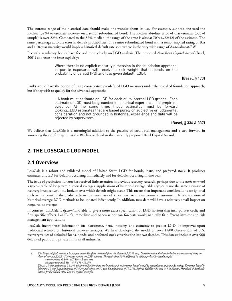
Figure 3 shows the timing of price observation of recovery estimates and the ultimate resolution of the claims. Brokerquotes on defaulted debt provide a far more timely recovery valuation relative to waiting to observe the completion ofcourt ordered resolution payments. Market quotes are commonly available in the period 15-to-60 days after default.However, if no pricing was available or if we felt that a price was not reliably stated, then it did not enter our dataset.

2. This date is not always well defined. As an example, bank loan covenants are commonly written with terms that are more sensitive to credit distress than those of bond debentures. Thus, different debt obligations of a single defaulted firm may officially default on different dates. The vast majority of securities in our dataset are quoted within the range of 15-to-60 days of the date assigned to initial default of the firm's public debt. Our study found no distinction in the quality or explicability of default prices across this 45-day range.

3. Contributed by Goldman Sachs, Citibank, BDS Securities, Loan Pricing Corporation, Merrill Lynch, and Lehman Brothers.

8

Although it is beyond the scope of this report, there have been several studies of the market's ability to price defaulted debtefficiently.4 These studies do not always show statistically significant results, but they consistently support the market'sefficient pricing of ultimate recoveries. At different times, Moody's has studied recovery estimates derived from both bid-side market quotes and discounted estimates of resolution value. Both methods have their advantages and disadvantages.We find, consistent with outside academic research, that these two tend to be unbiased estimates of each other.

3.2 Factor DescriptionsOver the course of model development, we considered the inclusion of a number of predictive variables. We includedfactors only if they have both a strong economic rationale and statistical significance.5

In all, the LossCalc models use nine factors to predict immediate LGD and a subset of eight factors to predict one-yearLGD. We grouped the factors into four categories as shown in Table 1 below. The table highlights the four broadcategories of predictive information: debt type and seniority, firm specific capital structure, industry, and macro economic.These factors have little intercorrelation and together make a significant and more accurate prediction of LGD. All factorsenter both LossCalc forecast horizons (i.e., immediate and one-year) with the single exception of the U.S. speculative-grade default rate. We chose to have this indicator enter only the immediate model.

FIGURE 3

Timeline of Default Recovery Estimation

This diagram illustrates the timing of the observation of recovery estimates, as represented by the prices of defaulted secu-rities and the ultimate resolution of the claims. Broker quotes on defaulted debt provide a far more timely recovery valuation relative to waiting to observe the completion of court ordered resolution payments. Market quotes are commonly available 15-to-60 days post-default. Final resolution takes 1¾ years at least half the time.

4. See Eberhart & Sweeney [1992], Wagner [1996] and Ward & Griepentrog [1993].5. Note that we also considered factors that were not included in the model due to either lower power than competing alternatives or data sufficiency issues. They are not

discussed here in detail. Some of these were: yields and spreads (e.g., BBB - AAA, Govt1, 2...10y, etc.), other macro factors (e.g., CPI, etc.), other financial ratios (e.g., EBIT / Sales, Current Liabilities / Current Assets, etc.), other instrument specific information (e.g., coupon, spread, etc.), and so forth.

TABLE 1: EXPLANATORY FACTORS IN THE LOSSCALC MODELS

Debt Type and Seniority

Historical average LGD by debt-type (loan, bond, and preferred stock) and seniority (secured, senior unsecured, subordinate, etc.).

Historical Averages

Firm-Specific Capital Structure

Seniority standing of debt in the firm's overall capital structure; this is the relative seniority of a claim. Note that this is different from the absolute seniority stated in Debt Type and Seniority above. The most senior obligation of a firm might be, for example, a subordi-nate note.

Seniority Standing

Firm leverage (Total Assets / Total Liabilities) Leverage

Industry

Moving average of normalized industry recoveries. We have here controlled for seniority class.

Industry Experience

Banking industry indicator Banking Indicator

"Technical" Defaults

Company Default + 15

Days+ 60 Days

Market Pricing (BidSide Quotes)

Final Resolution1¾ Years Median

Accounting of Resolution(Often with unknown values)

LOSSCALCTM: MODEL FOR PREDICTING LOSS GIVEN DEFAULT (LGD) 9

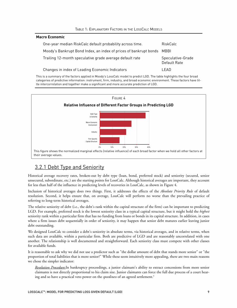
3.2.1 Debt Type and SeniorityHistorical average recovery rates, broken-out by debt type (loan, bond, preferred stock) and seniority (secured, seniorunsecured, subordinate, etc.) are the starting points for LossCalc. Although historical averages are important, they accountfor less than half of the influence in predicting levels of recoveries in LossCalc, as shown in Figure 4.

Inclusion of historical averages does two things. First, it addresses the effects of the Absolute Priority Rule of defaultresolution. Second, it helps ensure that, on average, LossCalc will perform no worse than the prevailing practice ofreferring to long-term historical averages.

The relative seniority of debt (i.e., the debt's rank within the capital structure of the firm) can be important to predictingLGD. For example, preferred stock is the lowest seniority class in a typical capital structure, but it might hold the highestseniority rank within a particular firm that has no funding from loans or bonds in its capital structure. In addition, in caseswhere a firm issues debt sequentially in order of seniority, it may happen that senior debt matures earlier leaving juniordebt outstanding.

We designed LossCalc to consider a debt's seniority in absolute terms, via historical averages, and in relative terms, whensuch data are available, within a particular firm. Both are predictive of LGD and are reasonably uncorrelated with oneanother. The relationship is well documented and straightforward. Each seniority class must compete with other classesfor available funds.

It is reasonable to ask why we did not use a predictor such as "the dollar amount of debt that stands more senior" or "theproportion of total liabilities that is more senior?" While these seem intuitively more appealing, there are two main reasonswe chose the simpler indicator:

Resolution Procedure:In bankruptcy proceedings, a junior claimant's ability to extract concessions from more seniorclaimants is not directly proportional to his claim size. Junior claimants can force the full due process of a court hear-ing and so have a practical veto power on the speediness of an agreed settlement.6

Macro Economic

One-year median RiskCalc default probability across time. RiskCalc

Moody's Bankrupt Bond Index, an index of prices of bankrupt bonds MBBI

Trailing 12-month speculative grade average default rate Speculative-Grade Default Rate

Changes in index of Leading Economic Indicators LEAD

This is a summary of the factors applied in Moody's LossCalc model to predict LGD. The table highlights the four broad categories of predictive information: instrument, firm, industry, and broad economic environment. These factors have lit-tle intercorrelation and together make a significant and more accurate prediction of LGD.

FIGURE 4

Relative Influence of Different Factor Groups in Predicting LGD

This figure shows the normalized marginal effects (relative influence) of each broad factor when we hold all other factors at their average values.

TABLE 1: EXPLANATORY FACTORS IN THE LOSSCALC MODELS

0% 10% 20% 30% 40%

Firm SpecificCapital Structure

Industry

Macro EconomicEnvironment

Debt Type

& Seniority

10

Availability of Data:Claim amounts at the time of default are not the same as original issuance/borrowing amounts. Inmany cases, obligations are paid down in part before the full maturity of the debt. Sinking funds (for bonds) andamortization schedules (for loans) are examples of this. Determining the exposure at default for many obligations canbe challenging, particularly for firms that pursue multiple funding channels. In many cases, this data is unavailable.Requiring such an extensive detailing of claims before being able to make any LGD forecast would be onerous fromboth a modeling and usage perspective.

3.2.2 Firm Specific Capital Structure: LeverageIntuitively, the capital structure of a firm is relevant to the funds available (in default) for the satisfaction of creditorclaims. Said another way, the assets to liabilities ratio acts like a coverage ratio of the funds available versus the claims to bepaid. A higher ratio of assets to liabilities is better.

However, leverage does not contribute to the prediction of LGD for secured credits. Such claims would look first to thevalue of their specific security and only secondarily seek satisfaction from the general funds of the defaulted firm.

3.2.3 IndustryResearchers frequently propose industry level segregation of recovery levels as being useful in recovery modeling.7 The ideais that an industry might consistently enjoy high recoveries or perhaps suffer recoveries that are consistently low acrosstime. Our test of this was to compile average industry recovery levels across time and test the statistical significance in theaverage's deviation from the overall average recovery.

We found this to work well for recoveries of bank defaults, which are consistently low across time. The rationale formodeling the banking industry by an indicator variable is as follows:

Seniority of Deposits over Public Debt: Deposits are commonly the majority of obligations of a bank and they enjoy a"super-seniority" position relative to public debt in bankruptcy.

Liquidity of Banks: Unlike the plant and equipment found in other industries, the financial assets and liabilities of abank are typically very short in duration and liquid. In response to this short-term nature (and to help stem systemicliquidity crisis), the Federal Reserve offers access to liquidity via the Fed's Discount Window. Thus, it is difficult forcreditors to "force" liquidity default on a bank that still has many good quality assets available to pay off its liabilities.Consequently, by the time banks default it is sometimes too late, when most of the good assets are insufficient.

Fed Forbearance: Historically, bank regulators have allowed insolvent banks to remain open. During the time that reg-ulators allow insolvent banks to remain open, banks use up their assets to pay off short-term liabilities and the avail-able asset coverage for long-term creditors falls proportionately.

However, we also found strong evidence of industry specific ebbs and flows in the recovery rates that differed in timebetween industries. We found that some industries would enjoy periods of prolonged superior recoveries, but fall well belowaverage recoveries at other times. A simple industry bump-up or notch-down, held constant over time, does not capture thisbehavior. To address this, we grouped firms into twelve broad industries and created moving averages of recoveries.8

3.2.4 Macro EconomicThe intuition behind the inclusion of macro economic variables is that defaulted debt prices tend to rise and fall togetheras a population rather than being fully independent of one other. Another way of saying this is that recoveries have positiveand significant intercorrelation within bands of time. This type of correlation has potentially material implications forportfolio calculations of Credit Value-at-Risk. The leading vendor models of Cr-VaR implicitly set this correlation to zeroand would thus understate Cr-VaR in this regard.

6. We tested this on a sub-population selected to have fully populated claim amount records. The best predictor of recoveries, both univariately and in combination with a core set of LossCalc regressors was a simple flag of standing the highest. As alternatives, we tested dollars (and log of dollars) of superior claims and proportion of supe-rior claims.

7. See Altman & Kishmore [1996] and Ivorski [1997] for broad recovery findings by industry and Borenstein & Rose [1995] for a single industry (airlines) case study.8. Industry categories: Banking, Consumer Products, Energy, Financial (Non-Bank), Hotel/Gaming/Leisure, Industrial, Media, Miscellaneous, Retail, Technology,

Transportation and Utilities.

LOSSCALCTM: MODEL FOR PREDICTING LOSS GIVEN DEFAULT (LGD) 11

3.2.4.1 One-Year RiskCalc Probability of Default

Moody's RiskCalc for Public companies can measure changes in the credit quality of corporate obligors with publiclytraded equity. RiskCalc is a hybrid model that combines two credit risk modeling approaches: (a) a structural model basedon Merton's options-theoretic view of firms; and (b) a statistical model determined through empirical analysis of historicalaccounting data. LossCalc uses time series of median RiskCalc PDs.

3.2.4.2 Moody's Bankrupt Bond Index

LossCalc uses Moody's Bankrupt Bond Index (MBBI), a monthly price index measuring the return of a broad cross-section of long-term public debt issues of corporations that are currently in bankruptcy. The bonds of defaulted ordistressed companies that have not yet filed for bankruptcy are not included in the index. MBBI includes both Moody's-rated and non-rated debt from U.S. and non-U.S. obligors, denominated in U.S. dollars.9

3.2.4.3 Trailing 12-month Speculative Grade Average Default Rates

While RiskCalc provides a measure of the outlook for default rates, we also found it useful to include a measure ofhistorical default rate behavior. We capture this through the inclusion of the trailing 12-month speculative grade defaultrate for Moody's rated firms. This factor did not exhibit strong predictive power for the one-year model and is thusincluded only in the immediate model where it was strongly significant.

3.2.4.4 Changes in Index of Leading Economic Indicators

We found that the change in Gross Domestic Product computed over the upcoming duration of default resolution wasstrongly predictive of recoveries. Of course, this future information could never be available for prediction. Nonetheless,this relationship indicates something of the process underlying recoveries.

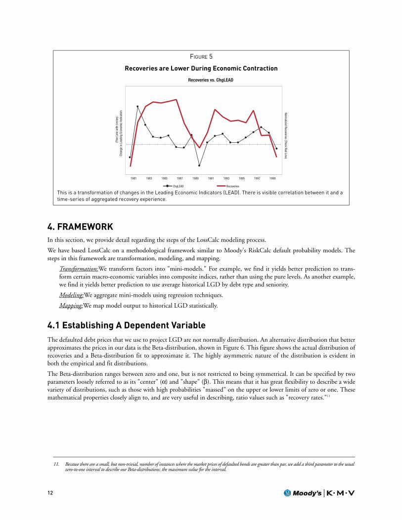
As a proxy, we chose a readily accessible series that seeks to address this same information, the Index of Leading EconomicIndicators.10 While its correlation with recoveries, as shown in Figure 5, is far from perfect, it is reasonable and carriessignificant predictive power. There is visible correlation between it and a time-series of aggregated recovery experience.

9. The MBBI historical series was revised in January 2000. Refer to "The Investment Performance of Bankrupt Corporate Debt Obligations", February 2000, Moody's Special Comment for details on this revision and about the construction of the MBBI.

10. The Conference Board, Inc. produces the Leading Economic Indicators. See their site at http://www.globalindicators.org, for details.

12

4. FRAMEWORKIn this section, we provide detail regarding the steps of the LossCalc modeling process.

We have based LossCalc on a methodological framework similar to Moody's RiskCalc default probability models. Thesteps in this framework are transformation, modeling, and mapping.

Transformation:We transform factors into "mini-models." For example, we find it yields better prediction to trans-form certain macro-economic variables into composite indices, rather than using the pure levels. As another example,we find it yields better prediction to use average historical LGD by debt type and seniority.

Modeling:We aggregate mini-models using regression techniques.

Mapping:We map model output to historical LGD statistically.

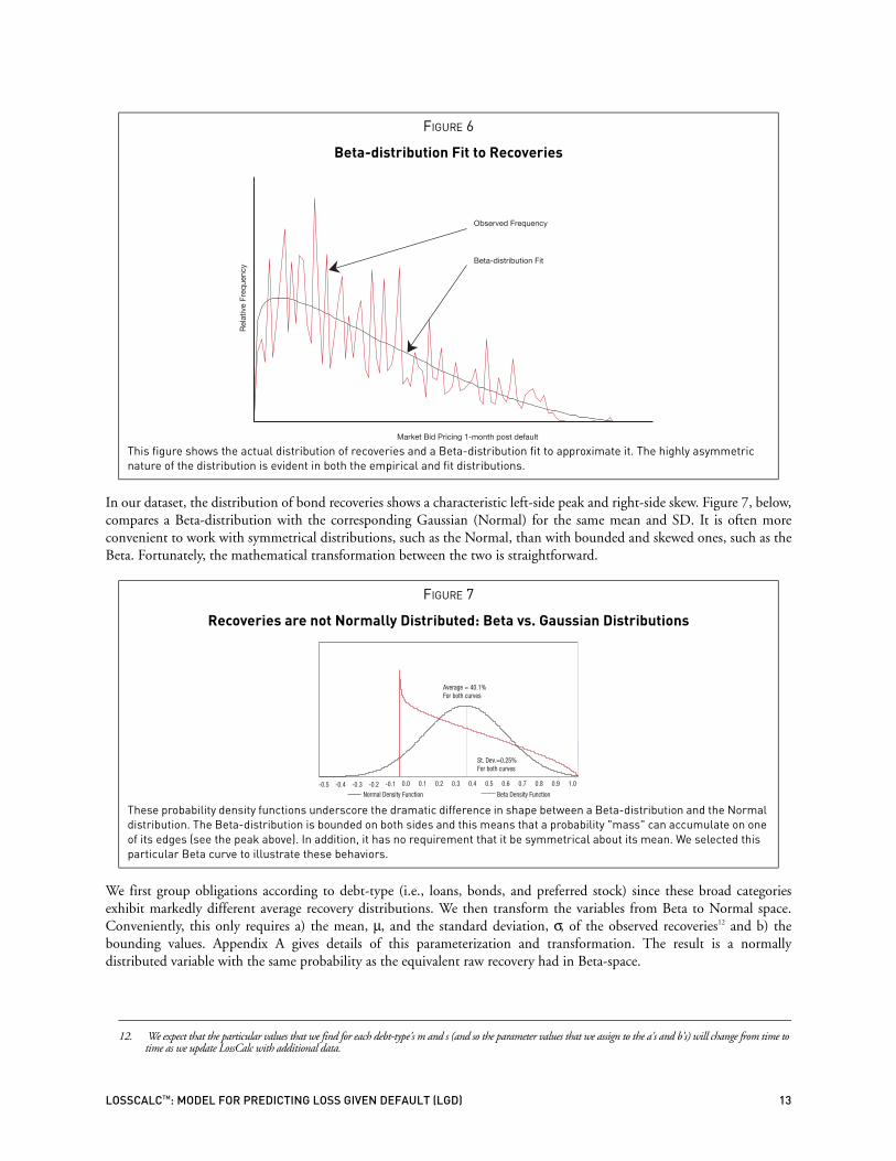
4.1 Establishing A Dependent VariableThe defaulted debt prices that we use to project LGD are not normally distribution. An alternative distribution that betterapproximates the prices in our data is the Beta-distribution, shown in Figure 6. This figure shows the actual distribution ofrecoveries and a Beta-distribution fit to approximate it. The highly asymmetric nature of the distribution is evident inboth the empirical and fit distributions.

The Beta-distribution ranges between zero and one, but is not restricted to being symmetrical. It can be specified by twoparameters loosely referred to as its "center" (α) and "shape" (β). This means that it has great flexibility to describe a widevariety of distributions, such as those with high probabilities "massed" on the upper or lower limits of zero or one. Thesemathematical properties closely align to, and are very useful in describing, ratio values such as "recovery rates."11

FIGURE 5

Recoveries are Lower During Economic Contraction

This is a transformation of changes in the Leading Economic Indicators (LEAD). There is visible correlation between it and a time-series of aggregated recovery experience.

11. Because there are a small, but non-trivial, number of instances where the market prices of defaulted bonds are greater than par, we add a third parameter to the usual zero-to-one interval to describe our Beta-distributions: the maximum value for the interval.

Recoveries vs. ChgLEAD

1981 1983 1985 1987 1989 1991 1993 1995 1997 1999

Chan

ge in

Lea

ding

Eco

nom

ic In

dica

tors

(Thi

n Li

ne w

ith c

ircle

s)Norm

alized Recoveries (Thick Red Line)

ChgLEAD Recoveries

LOSSCALCTM: MODEL FOR PREDICTING LOSS GIVEN DEFAULT (LGD) 13

In our dataset, the distribution of bond recoveries shows a characteristic left-side peak and right-side skew. Figure 7, below,compares a Beta-distribution with the corresponding Gaussian (Normal) for the same mean and SD. It is often moreconvenient to work with symmetrical distributions, such as the Normal, than with bounded and skewed ones, such as theBeta. Fortunately, the mathematical transformation between the two is straightforward.

We first group obligations according to debt-type (i.e., loans, bonds, and preferred stock) since these broad categoriesexhibit markedly different average recovery distributions. We then transform the variables from Beta to Normal space.Conveniently, this only requires a) the mean, µ, and the standard deviation, σ, of the observed recoveries12 and b) thebounding values. Appendix A gives details of this parameterization and transformation. The result is a normallydistributed variable with the same probability as the equivalent raw recovery had in Beta-space.

FIGURE 6

Beta-distribution Fit to Recoveries

This figure shows the actual distribution of recoveries and a Beta-distribution fit to approximate it. The highly asymmetric nature of the distribution is evident in both the empirical and fit distributions.

FIGURE 7

Recoveries are not Normally Distributed: Beta vs. Gaussian Distributions

These probability density functions underscore the dramatic difference in shape between a Beta-distribution and the Normal distribution. The Beta-distribution is bounded on both sides and this means that a probability "mass" can accumulate on one of its edges (see the peak above). In addition, it has no requirement that it be symmetrical about its mean. We selected this particular Beta curve to illustrate these behaviors.

12. We expect that the particular values that we find for each debt-type's m and s (and so the parameter values that we assign to the a's and b's) will change from time to time as we update LossCalc with additional data.

Market Bid Pricing 1-month post default

Rel

ativ

e Fr

eque

ncy

Observed Frequency

Beta-distribution Fit

-0.5 -0.4 -0.3 -0.2 -0.1 0.0 0.1 0.2 0.3 0.4 0.5 0.6 0.7 0.8 0.9 1.0

Normal Density Function Beta Density Function

St. Dev.=0.25%For both curves

Average = 40.1%For both curves

14

4.2 Transformation And Mini-modelingWe gained a great deal of insight by assessing predictive factors on a stand-alone (univariate) basis. We transform some ofthe input factors to make them better stand-alone predictors before assembling an "overall" model. If thesetransformations create a truly significant factor, then we typically rename its transformation a "mini-model."

In LossCalc for example, both the Seniority-Class ariable and the Industry LGDvariable are "mini-models." Each isindicative on a stand-alone basis as a measure of recovery values. Other instances of mini-modeling were less dramatic,such as a leverage ratio, logs, or changes versus levels in a time-series, etc. Two other model components are useful to note.

4.2.1 The Index of Macro ChangesLossCalc uses an index calculated by statistically weighting the changes in levels of various macro economic indicators intoa composite index, which is in effect an estimate of the average recovery that would be implied by these macro changesonly.13 We do this weighing as we step forward in time each month. This both maximizes its overall predictive power andminimizes month-to-month changes in the weighting.

4.2.2 Factor Inclusion by Seniority Class and IndustryThe model drops certain factors in certain cases. For example, although leverage is one of the nine predictive factors in theLossCalc model, it is not included in the case of financial institutions. These are typically highly leveraged with lendingand investment portfolios having very different implications than an industrial firm's plant and equipment.

Similarly, we do not consider leverage when assessing secured debt. The recovery value of a secured obligation dependsprimarily on the value of its collateral rather than the netted value of general corporate assets.

4.3 Modeling And Mapping: Explanation To PredictionThe modeling phase of the LossCalc methodology involves statistically determining the appropriate weights to use incombining the transformed variables and mini-models described in the previous section. The combination of all the abovepredictive factors is a linear weighted sum, derived using regression techniques. The model takes the additive form:

Where the xi are the transformed values and mini-models described above, the βι , are the weights and is the normalized ris the recovery. Note that at this point r is stated in "normalized space" and still needs to be transformed back into "dollarspace." So the final step is to apply the inverse of the Beta-distribution transformation (discussed above) to the three casesof loans, bonds, and preferred stock. See Appendix A for more details.

4.4 Confidence Interval EstimationLossCalc also provides an estimate of the confidence interval (i.e., upper and lower bounds) on the recovery prediction.Confidence intervals (CI) provide a range around the prediction within which we anticipate the actual value to fall aspecified percentage of the time. The width of a confidence interval provides information about the precision of theestimate. For example, we do not typically find that the actual value exactly matches the prediction every time. How far offmight it be?

An 80% confidence interval around that predicted value is the range (bounded by an upper bound and lower bound) inwhich we are confident the true value will fall 80% of the time. Therefore, we would only expect the actual future value tobe below the lower bound or above the upper bound, 20% of the time.

Confidence intervals have received surprisingly little attention in the recovery literature. Many investors are surprised tolearn of the relatively high variability around the estimates of recovery rates produced by tables, illustrated in Figure 2.

13. Note that this is similar in some ways to the creation of univariate default curves used in the RiskCalc models. In this case, the transformation involves a multivariate representation. (See, for example, Falkenstein & Boral [2000]).

r = α + β1x1 + β2x2 + β3x3 + ... + βkxk^

LOSSCALCTM: MODEL FOR PREDICTING LOSS GIVEN DEFAULT (LGD) 15

Although regression models produce a natural estimate of the (in-sample) confidence intervals, we found these relativelywide. We developed, estimated, and validated a conditional CI prediction approach that produced narrower ranges ofconfidence. In effect, a multi-dimensional lookup table results in narrower confidence intervals. The table has dimensionsfor debt type and seniority as well as others such as macro economic factors, etc. Each cell in the table containsinformation on the distribution of prediction errors for LossCalc. By using this table, we can calculate empirical upper andlower bounds of a confidence interval. This methodology was tested out of sample and produced robust results, asdiscussed in Section 5.

5. VALIDATION AND TESTINGThe primary goals of validation and testing are to:

• determine how well a model performs;

• ensure that a model has not been overfit and that its performance is reliable and well understood;

• confirm that the modeling approach, not just an individual model, is robust through time and credit cycles.

To validate the performance of LossCalc, we have used the approach adopted and refined by Moody's and used to validateRiskCalc, Moody's default prediction models. The methodology we use, termed walk forward validation, involves fitting amodel on one set of data from one time period and testing it on a subsequent period. We then repeat this process, movingthrough time until we have tested the model on all periods up to the present. Thus, we never use data to test the model thatwe used to fit its parameters and so we avoid over-fitting. We can also assess the behavior of the modeling approach overvarious economic cycles. Walk forward testing is a robust methodology that accomplishes the three goals set out above.

Model validation is an essential step to credit model development. We must take care to perform tests in a rigorous androbust manner while also guarding against unintended errors. For example, it is important to compare all models on thesame data. We have found that the same model may get different performance results on different datasets, even whenthere is no specific selection bias in choosing the data. To facilitate comparison, and avoid misleading results, we use thesame dataset to evaluate LossCalc and competing models.

Sobehart, Keenan, & Stein [2000] describe the walk-forward methodology more fully. Appendix B of this document givesa brief overview of the approach.

5.1 Alternative Recovery Models Used As BenchmarksThe standard practice in the market is to estimate LGD by some historical average. There are many variations in thedetails of how these averages are constructed: long-term versus moving window, by seniority class versus overall, dollarweighted versus simple (event) weighted. We chose two of these methodologies as being both representative and broadlyapplied. We then use these traditional approaches as benchmarks against which to measure the performance of theLossCalc models.

5.1.1 Table of Historical AveragesAs noted, the dominant paradigm for LGD estimation is historical averages. It is important to realize that the publishedresearch on recovery (e.g., Moody's annual default studied) typically presents statistics for an aggregated period. Thus,these type of reports cannot be used for walk forward testing since they include information that is often only availableafter a particular instrument defaulted. For example, Moody's studies, completed in 1996, 1998, 1999, and 2000 wouldcontain future information for much of the testing period.

We wanted to emulate the prevailing use of these tables — updating them, as one would step one year forward in timeeach year. Said another way, analysts understanding of the long-term historical recovery average evolves with each year'snew information. We tabulated these averages, for each debt-type, seniority grade, and year in our sample. This procedurereplicates the common practice of LGD estimation and, with Moody's sizable dataset, it represents a high qualityimplementation of this "classic lookup" approach.

16

5.1.2 The Historical Mean Recovery RateWe have also observed that many market participants use a simple historical average recovery rate as a recovery estimate.To emulate this measure, we recalculate the average historical recovery rate each year as well.

5.2 The Losscalc Validation TestsValidation testing for LossCalc is somewhat different from the testing procedure implemented for RiskCalc. This isbecause LossCalc produces an estimate of an amount (of recoveries) rather than some likelihood (of default). Therefore,LossCalc seeks to fit a continuous variable as opposed to predicting the binary outcome of default/no default. Thus, thediagnostics we use to evaluate its performance reflect this.

There are two important measures of the model. The first is accuracy: how well does the model predict actual lossesexperienced by an investor or lender? The second is efficiency: how wide are the confidence intervals on predictions?In general, these are related. Narrower confidence intervals typically (not always) arise from better prediction.Narrower confidence intervals allow better estimation of expected losses, Value-at-Risk, and (potentially lower)economic capital requirements.

In the next several sub-sections, we present measures of the LossCalc model performance in both the immediate and one-year cases. We compare LossCalc against both historical average approaches.

Since 1991 was the first year that we had enough data to build a sufficiently reliable model, unless otherwise stated, weused 1992 as the first out-of-sample year for which to predict. Following the walk-forward procedure, we constructed avalidation result set containing over 850 observations, representing over 500 different firms from Moody's extensivedatabase in the years 1992 - 2001. This result dataset was just under half of the total observations in the full dataset. It wasa representative sampling of rated and unrated public and private firms in all industries.

5.2.1 Prediction Error RatesAs a first measure of performance, we examined the error rate of the model. By convention, this is measured with anestimate of the mean squared error (MSE) of each model. The MSE is calculated as:

where ri and ri are the actual and estimated recoveries, respectively, on security i. The variable, n, is the number ofsecurities in the sample.

Models with lower MSE have smaller differences between the actual and predicted values and thus predict more closelythe acutal recovery.

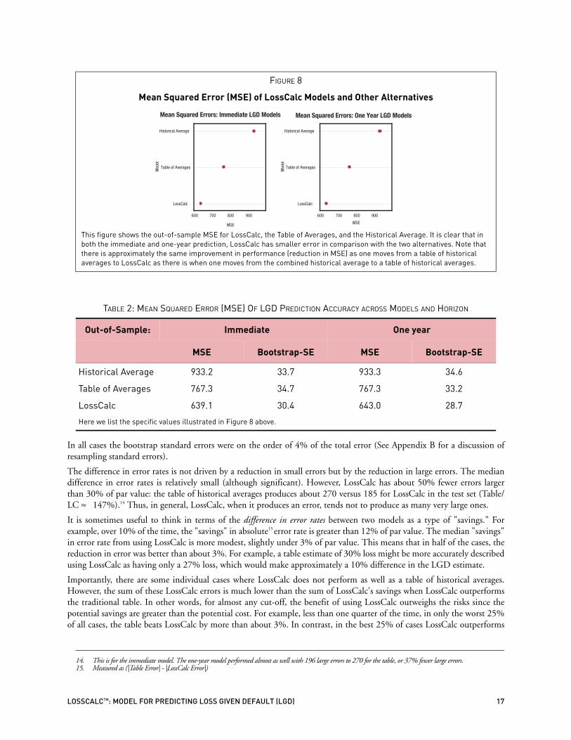
We note that there is approximately the same improvement in performanace (reduction in MSE) as one moves from thetable of historical averages to LossCalc as there is when one moves from a simple historical average to a table.

MSE = n - 1

∑ (ri - ri)2

LOSSCALCTM: MODEL FOR PREDICTING LOSS GIVEN DEFAULT (LGD) 17

In all cases the bootstrap standard errors were on the order of 4% of the total error (See Appendix B for a discussion ofresampling standard errors).

The difference in error rates is not driven by a reduction in small errors but by the reduction in large errors. The mediandifference in error rates is relatively small (although significant). However, LossCalc has about 50% fewer errors largerthan 30% of par value: the table of historical averages produces about 270 versus 185 for LossCalc in the test set (Table/LC ≈ 147%).14 Thus, in general, LossCalc, when it produces an error, tends not to produce as many very large ones.

It is sometimes useful to think in terms of the difference in error rates between two models as a type of "savings." Forexample, over 10% of the time, the "savings" in absolute15 error rate is greater than 12% of par value. The median "savings"in error rate from using LossCalc is more modest, slightly under 3% of par value. This means that in half of the cases, thereduction in error was better than about 3%. For example, a table estimate of 30% loss might be more accurately describedusing LossCalc as having only a 27% loss, which would make approximately a 10% difference in the LGD estimate.

Importantly, there are some individual cases where LossCalc does not perform as well as a table of historical averages.However, the sum of these LossCalc errors is much lower than the sum of LossCalc's savings when LossCalc outperformsthe traditional table. In other words, for almost any cut-off, the benefit of using LossCalc outweighs the risks since thepotential savings are greater than the potential cost. For example, less than one quarter of the time, in only the worst 25%of all cases, the table beats LossCalc by more than about 3%. In contrast, in the best 25% of cases LossCalc outperforms

FIGURE 8

Mean Squared Error (MSE) of LossCalc Models and Other Alternatives

This figure shows the out-of-sample MSE for LossCalc, the Table of Averages, and the Historical Average. It is clear that in both the immediate and one-year prediction, LossCalc has smaller error in comparison with the two alternatives. Note that there is approximately the same improvement in performance (reduction in MSE) as one moves from a table of historical averages to LossCalc as there is when one moves from the combined historical average to a table of historical averages.

TABLE 2: MEAN SQUARED ERROR (MSE) OF LGD PREDICTION ACCURACY ACROSS MODELS AND HORIZON

Out-of-Sample: Immediate One year

MSE Bootstrap-SE MSE Bootstrap-SE

Historical Average 933.2 33.7 933.3 34.6

Table of Averages 767.3 34.7 767.3 33.2

LossCalc 639.1 30.4 643.0 28.7

Here we list the specific values illustrated in Figure 8 above.

14. This is for the immediate model. The one-year model performed almost as well with 196 large errors to 270 for the table, or 37% fewer large errors.15. Measured as (|Table Error| - |LossCalc Error|)

600 700 800 900

MSE

LossCalc

Table of Averages

Historical Average

Mod

el

Mean Squared Errors: Immediate LGD Models

600 700 800 900

MSE

LossCalc

Table of Averages

Historical Average

Mod

el

Mean Squared Errors: One Year LGD Models

18

the table by saving over 7% or more. The ratio of error savings/cost at each point is in the range of 1.5 times to about 2times more savings than cost. Thus, LossCalc gives about 1.5 to 2 times more "savings" relative to error rate "cost."

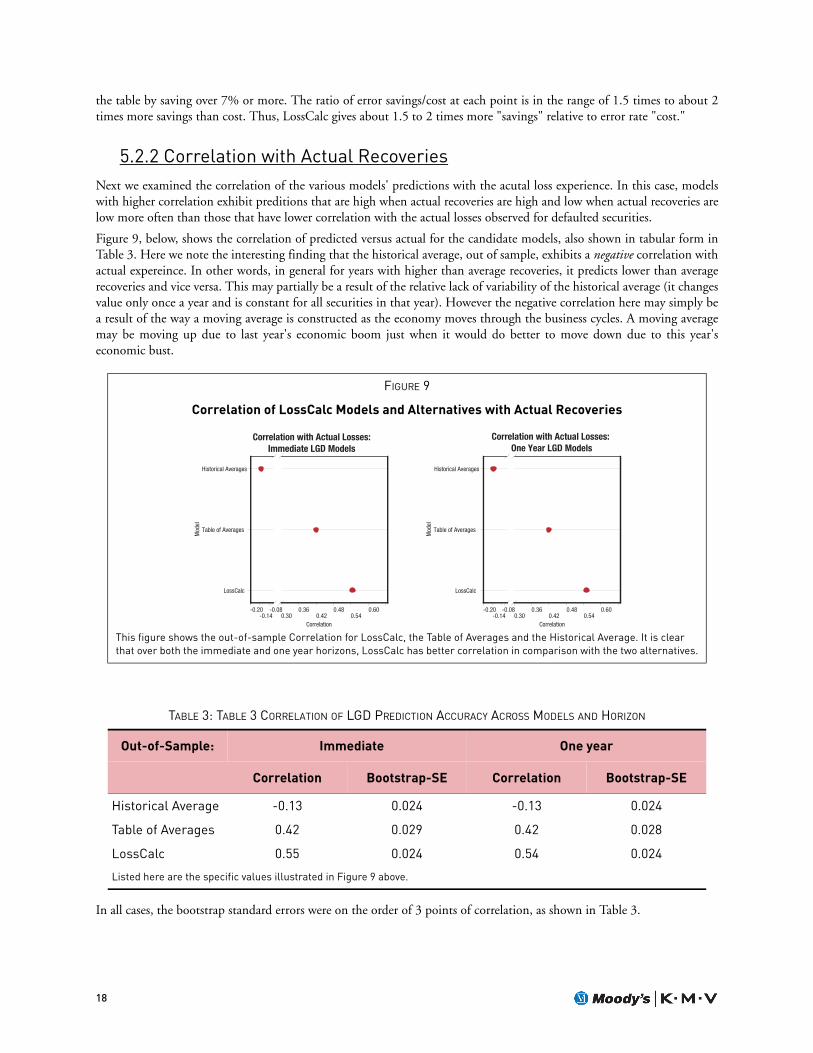
5.2.2 Correlation with Actual RecoveriesNext we examined the correlation of the various models' predictions with the acutal loss experience. In this case, modelswith higher correlation exhibit preditions that are high when actual recoveries are high and low when actual recoveries arelow more often than those that have lower correlation with the actual losses observed for defaulted securities.

Figure 9, below, shows the correlation of predicted versus actual for the candidate models, also shown in tabular form inTable 3. Here we note the interesting finding that the historical average, out of sample, exhibits a negative correlation withactual expereince. In other words, in general for years with higher than average recoveries, it predicts lower than averagerecoveries and vice versa. This may partially be a result of the relative lack of variability of the historical average (it changesvalue only once a year and is constant for all securities in that year). However the negative correlation here may simply bea result of the way a moving average is constructed as the economy moves through the business cycles. A moving averagemay be moving up due to last year's economic boom just when it would do better to move down due to this year'seconomic bust.

In all cases, the bootstrap standard errors were on the order of 3 points of correlation, as shown in Table 3.

FIGURE 9

Correlation of LossCalc Models and Alternatives with Actual Recoveries

This figure shows the out-of-sample Correlation for LossCalc, the Table of Averages and the Historical Average. It is clear that over both the immediate and one year horizons, LossCalc has better correlation in comparison with the two alternatives.

TABLE 3: TABLE 3 CORRELATION OF LGD PREDICTION ACCURACY ACROSS MODELS AND HORIZON

Out-of-Sample: Immediate One year

Correlation Bootstrap-SE Correlation Bootstrap-SE

Historical Average -0.13 0.024 -0.13 0.024

Table of Averages 0.42 0.029 0.42 0.028

LossCalc 0.55 0.024 0.54 0.024

Listed here are the specific values illustrated in Figure 9 above.

-0.20-0.14

-0.080.30

0.360.42

0.480.54

0.60

Correlation

LossCalc

Table of Averages

Historical Averages

Mod

el

Correlation with Actual Losses: One Year LGD Models

-0.20-0.14

-0.080.30

0.360.42

0.480.54

0.60

Correlation

LossCalc

Table of Averages

Historical Averages

Mod

el

Correlation with Actual Losses: Immediate LGD Models

LOSSCALCTM: MODEL FOR PREDICTING LOSS GIVEN DEFAULT (LGD) 19

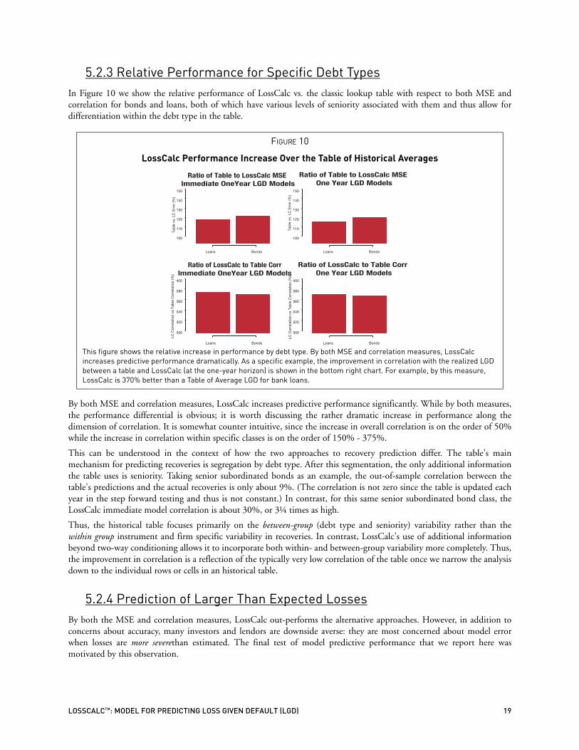
5.2.3 Relative Performance for Specific Debt TypesIn Figure 10 we show the relative performance of LossCalc vs. the classic lookup table with respect to both MSE andcorrelation for bonds and loans, both of which have various levels of seniority associated with them and thus allow fordifferentiation within the debt type in the table.

By both MSE and correlation measures, LossCalc increases predictive performance significantly. While by both measures,the performance differential is obvious; it is worth discussing the rather dramatic increase in performance along thedimension of correlation. It is somewhat counter intuitive, since the increase in overall correlation is on the order of 50%while the increase in correlation within specific classes is on the order of 150% - 375%.

This can be understood in the context of how the two approaches to recovery prediction differ. The table's mainmechanism for predicting recoveries is segregation by debt type. After this segmentation, the only additional informationthe table uses is seniority. Taking senior subordinated bonds as an example, the out-of-sample correlation between thetable's predictions and the actual recoveries is only about 9%. (The correlation is not zero since the table is updated eachyear in the step forward testing and thus is not constant.) In contrast, for this same senior subordinated bond class, theLossCalc immediate model correlation is about 30%, or 3¼ times as high.

Thus, the historical table focuses primarily on the between-group (debt type and seniority) variability rather than thewithin group instrument and firm specific variability in recoveries. In contrast, LossCalc's use of additional informationbeyond two-way conditioning allows it to incorporate both within- and between-group variability more completely. Thus,the improvement in correlation is a reflection of the typically very low correlation of the table once we narrow the analysisdown to the individual rows or cells in an historical table.

5.2.4 Prediction of Larger Than Expected LossesBy both the MSE and correlation measures, LossCalc out-performs the alternative approaches. However, in addition toconcerns about accuracy, many investors and lendors are downside averse: they are most concerned about model errorwhen losses are more severethan estimated. The final test of model predictive performance that we report here wasmotivated by this observation.

FIGURE 10

LossCalc Performance Increase Over the Table of Historical Averages

This figure shows the relative increase in performance by debt type. By both MSE and correlation measures, LossCalc increases predictive performance dramatically. As a specific example, the improvement in correlation with the realized LGD between a table and LossCalc (at the one-year horizon) is shown in the bottom right chart. For example, by this measure, LossCalc is 370% better than a Table of Average LGD for bank loans.

100

110

120

130

140

150

Ratio of Table to LossCalc MSE Immediate OneYear LGD Models

Tab

le v

s. L

C E

rror

(%)

Loans Bonds Loans Bonds

Loans BondsLoans Bonds

100

110

120

130

140

150

Ratio of Table to LossCalc MSE One Year LGD Models

Tab

le v

s. L

C E

rror

(%)

300

320

340

360

380

400

Ratio of LossCalc to Table Corr Immediate OneYear LGD Models

LC C

orre

latio

n vs

Tab

le C

orre

latio

n (%

)

300

320

340

360

380

400

Ratio of LossCalc to Table Corr One Year LGD Models

LC C

orre

latio

n vs

Tab

le C

orre

latio

n (%

)

20

The test was designed to evaluate each model's ability to predict cases in which actual losses were greater than historicalexpectations.

The test proceded as follows:

1. Using the most recent information available up to the time of a default, we first labeled each record with repsect towhether the actual loss experienced was greater or less than the historical mean loss for all instruments to date.

2. We then ordered all out-of-sample predictions for each model from largest predicted loss to smallest predicted loss.

3. Finally, we calculated the percentage of larger than average losses each model captured in its ordering using standardpower tests.

This approach allowed us to convert the model performance to a binary measure which in turn allowed us to use familiarmetrics and diagnostis such as power curves and power statistics to measure performance.

All things being equal, if a model was powerful at predicting larger than average losses, we would expect the largest losspredictions to be associated with the actual above average losses and the lowest loss predictions to be associated with belowaverage losses. (On a power curve, this would result in the curve for a good model being bowed out towards theNorthwestern corner of the chart. The random model would be a 45º line showing no difference in association betweenhigh and low ranked obligations.) While, this metric coarsens somewhat the acutal model output, we have found that itprovides a valuable perspective in evaluating recovery model performance.

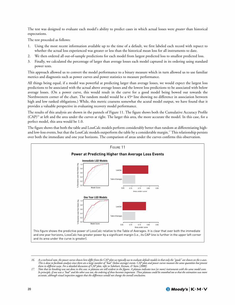
The results of this analysis are shown in the pannels of Figure 11. The figure shows both the Cumulative Accuracy Profile(CAP)16 at left and the area under the curves at right. The larger this area, the more accurate the model. In this case, for aperfect model, this area would be 1.0.

The figure shows that both the table and LossCalc models perform considerably better than random at differentiating high-and low-loss events, but that the LossCalc models outperform the table by a considerable margin.17 This relationship persistsover both the immediate and one year horizons. The comparison of areas under the curves confirms this observation.

16. As a technical note, the power curves shown here differ from the CAP plots we typically use to evaluate default models in that only the "goods" are shown on the x-axes. This is done to facilitate analysis since there are a large number of "bad" (below average) events. CAP plots and power curves measure the same quantities but present them in different ways. For a detailed discussion of CAP plots, refer to Sobehart, Keenan, & Stein [2000].

17. Note that tie breaking was not done in this case, so plateaus are still evident in the figures. A plateau indicates two (or more) instruments with the same model score. In principle, if one was a "bad" and the other was not, the ordering of these becomes important. These plateaus could be smoothed too so that the estimation was more accurate, although visual inspection suggests that the differences would not change the overall conclusions.

FIGURE 11

Power at Predicting Higher than Average Loss Events

This figure shows the predictive power of LossCalc relative to the Table of Averages. It is clear that over both the immediate and one year horizons, LossCalc has greater power by a significant margin (i.e., its CAP line is further in the upper left corner and its area under the curve is greater).

Model Score% R

ecov

erie

s Lo

wer

than

His

toric

Avg

.

0.0

0.2

0.4

0.6

0.8

1.0

Immediate LGD Models

0.65 0.70 0.75 0.80 0.85

Area under curve

Table of Averages

Table of Averages

LossCalc

Model Score% R

ecov

erie

s Lo

wer

than

His

toric

Avg

.

0.0

0.2

0.4

0.6

0.8

1.0

One Year LGD Models

0.65 0.70 0.75 0.80 0.85Area under curve

LossCalc

LOSSCALCTM: MODEL FOR PREDICTING LOSS GIVEN DEFAULT (LGD) 21

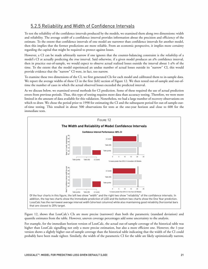
5.2.5 Reliability and Width of Confidence IntervalsTo test the reliability of the confidence intervals produced by the models, we examined them along two dimensions: widthand reliability. The average width of a confidence interval provides information about the precision and efficiency of theestimate. To the extent that confidence intervals of one model are narrower than confidence intervals for another model,then this implies that the former predictions are more reliable. From an economic perspective, it implies more certaintyregarding the capital that might be required to protect against losses.

However, a CI can be made arbitrarily narrow if one ignores that the counter-balancing constraint is the reliability of amodel's CI at actually predicting the true interval. Said otherwise, if a given model produces an a% confidence interval,then in practice out-of-sample, we would expect to observe actual realized losses outside the interval about 1-a% of thetime. To the extent that the model experienced an undue number of actual losses outside its "narrow" CI, this wouldprovide evidence that the "narrow" CI were, in fact, too narrow.

To examine these two dimensions of the CI, we first generated CIs for each model and calibrated them to in-sample data.We report the average widths of these CI in the first (left) section of Figure 12. We then tested out-of-sample and out-of-time the number of cases in which the actual observed losses exceeded the predicted interval.

As we discuss below, we examined several methods for CI prediction. Some of these required the use of actual predictionerrors from previous periods. Thus, this type of testing requires more data than accuracy testing. Therefore, we were morelimited in the amount of data available for this validation. Nonetheless, we had a large number of recovery observations onwhich to draw. We chose the period prior to 1998 for estimating the CI and the subsequent period for out-of-sample-out-of-time testing. This resulted in about 500 observations for tests at the one-year horizon and close to 600 for theimmediate tests.

Figure 12, shows that LossCalc's CIs are more precise (narrower) than both the parametric (standard deviation) andquantile estimates from the table. However, uneven coverage percentages add some uncertainty to the analysis.

For example, for the immediate horizon version of LossCalc, the actual out-of-sample coverage of the historical table washigher than LossCalc signalling not only a more precise estimation, but also a more efficient one. However, the 1-yearversion shows a slightly higher out-of-sample coverage than the historical table indicating that the width of the CI couldprobably have been made tighter. Similarly, the width of the parametric CI for the table are likely optimistically narrow,

FIGURE 12

The Width and Reliability of Model Confidence Intervals

Of the four charts in this figure, the left two show "width" and the right two show "reliability" of the confidence intervals. In addition, the top two charts show the Immediate prediction of LGD and the bottom two charts show the One Year prediction. LossCalc has the narrowest average interval width (shortest columns) while also maintaining good reliability (horizontal bars that are closest to 20% target.

60

65

70

75

80

85

90

Mea

n %

CI w

idth

: Ins

tant

aneo

us

Table (pctile) Table (SD) LC (cond)

0 5 10 15 20 25

% losses greater than 80% CI: Immediate LGD Models

60

65

70

75

80

85

90

Mea

n %

con

fiden

ce in

terv

al w

idth

:One

yea

r

Table (pctile) Table (SD) LC (cond)

Table (pctile)

Table (SD)

LC (cond)

Table (pctile)

Table (SD)

LC (cond)

0 5 10 15 20 25

% losses greater than 80% CI: One Year LGD Models

Confidence Interval Performance: 80% CI

22

due to the higher than expected number of cases outside the CI. Unfortuately, there is no way to anticipate such variancesfrom the expected CI a priori.

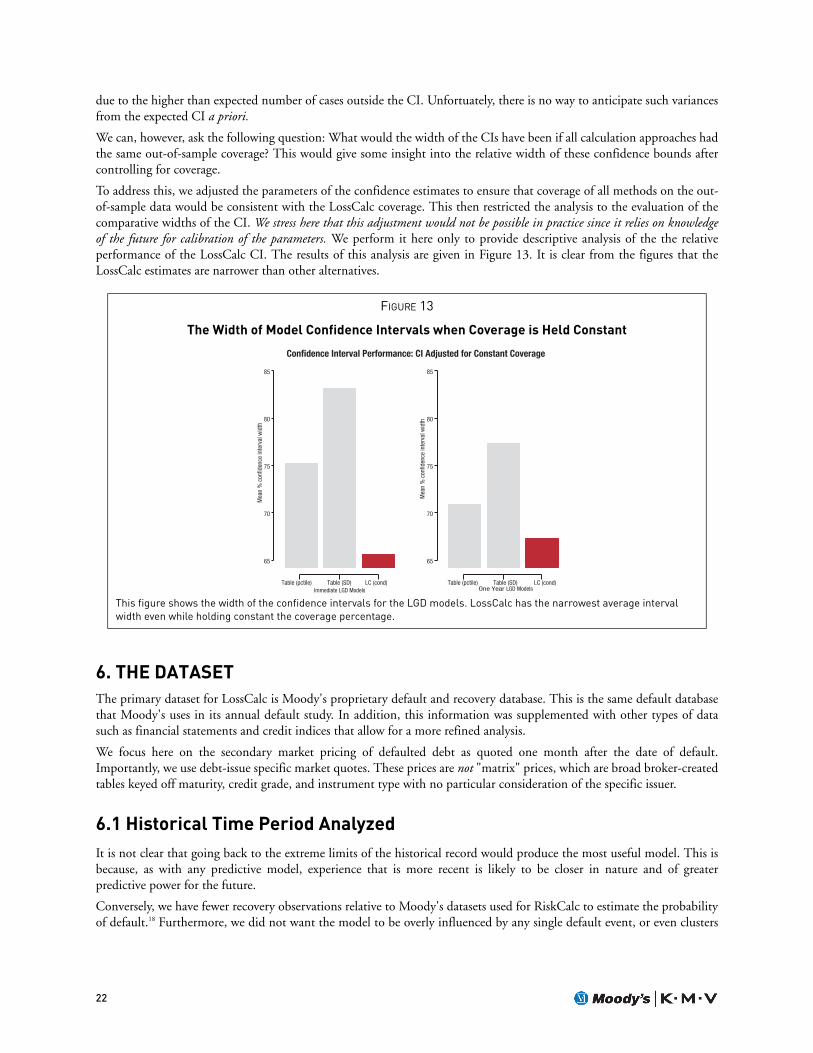
We can, however, ask the following question: What would the width of the CIs have been if all calculation approaches hadthe same out-of-sample coverage? This would give some insight into the relative width of these confidence bounds aftercontrolling for coverage.

To address this, we adjusted the parameters of the confidence estimates to ensure that coverage of all methods on the out-of-sample data would be consistent with the LossCalc coverage. This then restricted the analysis to the evaluation of thecomparative widths of the CI. We stress here that this adjustment would not be possible in practice since it relies on knowledgeof the future for calibration of the parameters. We perform it here only to provide descriptive analysis of the the relativeperformance of the LossCalc CI. The results of this analysis are given in Figure 13. It is clear from the figures that theLossCalc estimates are narrower than other alternatives.

6. THE DATASETThe primary dataset for LossCalc is Moody's proprietary default and recovery database. This is the same default databasethat Moody's uses in its annual default study. In addition, this information was supplemented with other types of datasuch as financial statements and credit indices that allow for a more refined analysis.

We focus here on the secondary market pricing of defaulted debt as quoted one month after the date of default.Importantly, we use debt-issue specific market quotes. These prices are not "matrix" prices, which are broad broker-createdtables keyed off maturity, credit grade, and instrument type with no particular consideration of the specific issuer.

6.1 Historical Time Period AnalyzedIt is not clear that going back to the extreme limits of the historical record would produce the most useful model. This isbecause, as with any predictive model, experience that is more recent is likely to be closer in nature and of greaterpredictive power for the future.

Conversely, we have fewer recovery observations relative to Moody's datasets used for RiskCalc to estimate the probabilityof default.18 Furthermore, we did not want the model to be overly influenced by any single default event, or even clusters

FIGURE 13

The Width of Model Confidence Intervals when Coverage is Held Constant

This figure shows the width of the confidence intervals for the LGD models. LossCalc has the narrowest average interval width even while holding constant the coverage percentage.

65

70

75

80

85

Mea

n %

con

fiden

ce in

terv

al w

idth

Table (pctile) Table (SD) LC (cond)Immediate LGD Models

65

70

75

80

85

Mea

n %

con

fiden

ce in

terv

al w

idth

Table (pctile) Table (SD) LC (cond)One Year LGD Models

Confidence Interval Performance: CI Adjusted for Constant Coverage

LOSSCALCTM: MODEL FOR PREDICTING LOSS GIVEN DEFAULT (LGD) 23

of closely related defaults. This would argue that we should use as much data as possible, which would mean going backfar in time.

Two considerations framed our selection of the historical period. First, we felt that the full specification and validation ofour model could only be achieved satisfactorily if one or more (in the case of LossCalc, two) full economic cycles areincluded in the dataset. This criterion was motivated by our early studies, which found that the credit cycle was a strongdeterminer of recoveries. Second, our research also indicated that firm-level capital structure was also predictive ofrecovery levels. To tailor our recovery estimates to the details of specific firms, we deemed it highly desirable to have accessto financial statement information.

For both of these reasons, the period we used was Jan-1981 to the present. This period covers two full credit cycles.

6.2 Scope Of Geographic Coverage And Legal DomainClearly, bankruptcy laws vary markedly across legal domains. UK law strongly seeks to protect creditors. French law doesnot recognize the priority of claims of specifically identified security. Some domains allow creditors to file a petition forinsolvency. And this is just a sampling of the diversity of liquidation rules.19 Therefore, for this version of LossCalc, wehave chosen to restrict the scope of the model to U.S. debt obligations only.

Having said this, as we move foreword and fit future versions of LossCalc to other domains, we anticipate that many ofour findings will hold.

6.3 Scope Of Firm Types And Instrument CategoriesSeniority standing is especially important to this version of LossCalc because we are focusing exclusively on U.S.recoveries. American bankruptcy law applies the concept of the Absolute Priority Rule, which states that more seniorclaimants must be fully satisfied before more junior claimants can start to receive any of the defaulted firm's liquidation/reorganization value. In practice, the actions in bankruptcy proceeding are more complicated,20 but this guiding principalmakes debt's seniority standing a leading component of recovery rate estimation.

Our dataset includes three broad debt instrument types: a) bank loans, b) public bonds, and c) preferred stock. Withinloans, there are two seniority grades: "senior secured," which are the more numerous, and "senior unsecured." Publicbonds subdivide into more seniority classes:

• senior secured;

• senior unsecured;

• senior subordinated;

• subordinated; and

• junior subordinated.

In addition to these five broad classes, we break out two specialized classes: corporate mortgages which are a kind of seniorsecured bond plus industrial revenue bonds (IRBs), which are a kind of senior unsecured bond.

Parenthetically, we make no distinction between the different types of preferred stock. In normal times, various factorsmake a real difference in the traded valuations of preferred stock. These include:

• fixed/floating rate payments;

• cumulative versus non-cumulative dividends; and

• convertibility.

None of these factors above is explicitly mentioned in the bankruptcy code. However, cumulative dividends may be astrong analogy with accrued interest for bonds, which are included in defaulted debt claims. As part of our continuingLGD research, we hope to assess whether bankruptcy courts act on this.

18. By definition, at the obligor level, the number of recovery observations is less than (or equal to) the number of default observations. There cannot be a recovery unless there has been a default observation. By comparison, RiskCalc has far more observations than LossCalc. However, a single default can also produce several instrument-level recovery observations if the obligor has multiple classes of debt outstanding.

19. See West & de Bodard [2000a,b,c] and Bartlett [1999].20. See Mann [1997] for a discussion of the common use and legal treatment of differing seniority classes and Stumpp, et. al. [1977] for a detailing of bank loan structure

and collateral.

24

As a final detail, we note that in the case of medium term note programs (MTNs), which are characterized by a largenumber of small issues, we consolidate the many individual issues into a single recovery observation per default event. Therecovery rate realized for this proxy observation is the simple average of all the individual issuances. It happens that therewas never large variability in the recovery estimates across issues within a single MTN program.

7. CONCLUSIONIn this report, we described the research done to develop LossCalc, Moody's loss given default (LGD) model. LossCalc isa multi-factor statistical model developed using a database of over 1800 defaulted instruments. It produces LGD estimatesfor bonds, syndicated loans, and preferred stock. LossCalc assesses information on four levels of analysis, including thecharacteristics of the instrument, the capital structure of the firm, and macro factors at both the economy and industry level.

The issue of prediction horizon for LGD is one that has not received much attention due to the largely static nature of thedominant historical average approach. This implicitly ignores the effects of the credit cycle and other time-varyingenvironmental factors. LossCalc, by its dynamic nature, allows for a much more exact specification of LGD horizon andproduces estimates on an immediate and one-year horizon.

We conducted extensive out-of-sample out-of-time validation of this model to determine how well it performed atpredicting LGD compared to alternative approaches. The results of this benchmarking show that the model performsbetter than common alternatives such as an overall historical average of LGD or a table of average LGDs. LossCalc'sperformance is superior in terms of both out-of-sample out-of-time prediction error and correlation of the predictionswith actual recovery experience. The model was also better at identifying low recoveries than historical average methodsand had fewer large errors.

Since risk management applications place particular demand upon the estimation of parameter uncertainty, we havedeveloped a conditional confidence interval prediction approach that results in narrower confidence intervals than alternativeapproaches. In validation testing, these intervals also more accurately represented the true variability of actual recoveries.

Combining the results of Moody's two models, RiskCalc for default probabilities and LossCalc for recovery rates, isnatural. With this combination, a risk manager can estimate the expected credit losses of an instrument, given knowledgeof the exposure amount. This is a much more complete portrayal of credit risk than probability of default alone.

Estimation of the average (mean expected) losses due to credit is commonly used to:

1. set reserve requirements for doubtful accounts;

2. establish minimum pricing levels at which new credit exposures to an obligor may be undertaken;

3. price credit risky instruments such as corporate bonds or credit default swaps; and

4. calculate risk-adjusted performance measures such as RAROC.

LossCalc's estimate of the downside confidence bound of LGD (an 80% two-tailed confidence interval) gives greatermeaning, consistency, and guidance to stressing recovery rate estimates and for provisioning.

LossCalc represents a robust and validated model of United States LGD for the debt types it covers. We believe that thisis a productive step forward in answering the call for rigor that the BIS has outlined in the recently proposed BaselCapital Accord.

LOSSCALCTM: MODEL FOR PREDICTING LOSS GIVEN DEFAULT (LGD) 25

APPENDIX A: BETA TRANSFORMATION TO NORMALIZE LOSS DATATo create an approximately normally distributed dependent variable from the raw observations of recovery, we firstconfirmed that defaulted debt valuations were approximately Beta distributed. There is no theoretical reason that this isthe "correct" shape of the defaulted debt prices, but previous studies have concluded that its characteristics make the Betaa reasonable description of the empirical shape.

Beta-distributions are described in this case by an upper and lower bound and by two shape parameters, α and β. Mostcommonly, it is naturally bounded between zero and one; its mean can be any value strictly within its range. Theconversion of the Beta distributed recovery values to a more normally distribution dependent variable is explicitly definedas follows:

The sub-notation "d" is only used to emphasize that LossCalc fits each debt-type to its own distribution.

Thus, much of the distributions of our three disparate separate asset classes can be captured by specifying only two shapeparameter values: the α and the β of each Beta-distribution. It is also possible, through algebraic manipulation, to specifythe Beta-distribution that simply matches the mean and standard deviation, which are functions of the shape andboundary parameters.

Mathematically, a Beta-distribution is a function of Gamma distributions. With the lower bound set to zero, thedistribution can be described as follows:

The shape parameters can be derived in a variety of ways. For example, the following give them in terms of populationmean and standard deviation.

Conversely, given Beta-distribution parameters, it is straightforward to calculate the mean and standard deviation.

Dependent Variable = Yi = N -1[Betadist(RecovRti, αd, βd, Min, Maxd]

whereRecovRt = min(Max - ε, observed recovery rate) ε = some small value

αd = The Beta Distribution's center parameter

βd = The Beta Distribution's shape parameter

Min = Set to zero for all cases

Maxd = Set to 1.1 for bonds, but otherwise is 1.0

d = {loans, bonds, preferred stock}

Beta (x, α, β, Min = 0, Max) = Γ(α + β)Γ(α)Γ(β)

x

Max

1

Maxx

Max1 - ( ) ( ) ( )β − 1α − 1

α = β = α andµ

max [µ (Max - µ)

Max σ2 ]- 1 [ ]µMax - 1

and σ = αβ

(α + β)2 + (1 + α + β)MaxMaxµ =

αα + β

26

APPENDIX B: AN OVERVIEW OF THE VALIDATION APPROACHTo validate the performance of LossCalc, we have used the approach adopted and refined by Moody's and used to validateMoody's quantitative default prediction models (RiskCalc). The approach, termed walk forward validation, is a robustmeans for ensuring that:

• models have not been "over-fit" to the data;

• future performance can be well understood; and

• the modeling approach, as well as any individual model produced by it, is robust through time and credit cycles.

We give only a brief overview of the methodology here; a fuller description is detailed in Sobehart, Keenan, & Stein [2000].21

B.1. Controlling For "Over Fitting" Risk: Walk-forward TestingIn order to avoid embedding unwanted sample dependency, we have found it useful to develop and validate models usingsome type of out-of-sample, out-of-universe and out-of-time testing approach on panel or cross-sectional datasets.22

However, such an approach can generate false impressions about reliability of a model if done incorrectly. "Hold out"testing can sometimes miss important model problems, particularly when processes vary over time, as credit risk does.23

Dhar & Stein [1997] suggest a framework for framing these issues as well as providing a more detailed discussion andsome examples from finance.

Our testing approach is designed to test models in a realistic setting, emulating closely the manner in which the modelswould be used in practice. The procedure we describe is often referred to in the trading model literature as "walk-forward"testing.

The walk-forward procedure works as follows:

1. Select a year, for example, 1991.

2. Fit the model using all the data available on or before the selected year.

3. Once the model's form and parameters are established for the selected period, generate the model outputs for all ofthe firms available during the following year (in this example 1992). Note that these are out-of-time and generallyout-of-sample.

4. Save the prediction as part of a result set.5. Now move the window up one year (e.g.: to 1992) so that all the data through that year can be used for fitting and

the data for the following year can be used for testing.

6. Repeat steps (2) to (5) adding the new predictions to the result set.

Collecting all the out-of-sample and out-of-time model predictions produces a set of model performances. This validationresult set can then be used to analyze the performance of the model in more detail.

Note that this approach simulates, as closely as possible given the limitations of the data, the process by which the modelwill actually be used in practice. Each year, the model is refit and used to predict recoveries one year hence. The walk-forward validation process is outlined in Figure 14.

21. Much of what follows was adapted from Sobehart, Keenan, & Stein [2000].22. A panel dataset contains observations over time on many individuals. A cross sectional dataset contains one observation on many individuals.23. See, for example, Mensah [1984].

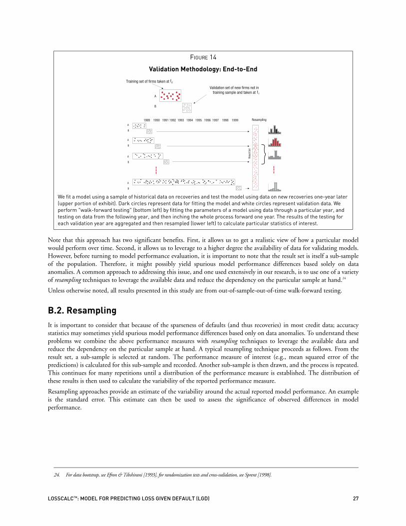
LOSSCALCTM: MODEL FOR PREDICTING LOSS GIVEN DEFAULT (LGD) 27

Note that this approach has two significant benefits. First, it allows us to get a realistic view of how a particular modelwould perform over time. Second, it allows us to leverage to a higher degree the availability of data for validating models.However, before turning to model performance evaluation, it is important to note that the result set is itself a sub-sampleof the population. Therefore, it might possibly yield spurious model performance differences based solely on dataanomalies. A common approach to addressing this issue, and one used extensively in our research, is to use one of a varietyof resampling techniques to leverage the available data and reduce the dependency on the particular sample at hand.24

Unless otherwise noted, all results presented in this study are from out-of-sample-out-of-time walk-forward testing.

B.2. ResamplingIt is important to consider that because of the sparseness of defaults (and thus recoveries) in most credit data; accuracystatistics may sometimes yield spurious model performance differences based only on data anomalies. To understand theseproblems we combine the above performance measures with resampling techniques to leverage the available data andreduce the dependency on the particular sample at hand. A typical resampling technique proceeds as follows. From theresult set, a sub-sample is selected at random. The performance measure of interest (e.g., mean squared error of thepredictions) is calculated for this sub-sample and recorded. Another sub-sample is then drawn, and the process is repeated.This continues for many repetitions until a distribution of the performance measure is established. The distribution ofthese results is then used to calculate the variability of the reported performance measure.

Resampling approaches provide an estimate of the variability around the actual reported model performance. An exampleis the standard error. This estimate can then be used to assess the significance of observed differences in modelperformance.

FIGURE 14

Validation Methodology: End-to-End

We fit a model using a sample of historical data on recoveries and test the model using data on new recoveries one-year later (upper portion of exhibit). Dark circles represent data for fitting the model and white circles represent validation data. We perform "walk-forward testing" (bottom left) by fitting the parameters of a model using data through a particular year, and testing on data from the following year, and then inching the whole process forward one year. The results of the testing for each validation year are aggregated and then resampled (lower left) to calculate particular statistics of interest.

24. For data bootstrap, see Efron & Tibshirani [1993], for randomization tests and cross-validation, see Sprent [1998].

1989 1990 1991 1992 1993 1994 1995 1996 1997 1998 1999

llllll

Training set of firms taken at t0

Validation set of new firms not in training sample and taken at t1

-2 -1 0 1

0.0

0.2

0.4

0.6

Error

-3 -2 -1 0 1 2 3

0.0

0.05

0.10

0.15

0.20

0.25

0.30

Error

-3 -2 -1 0 1 2 3

0.0

0.1

0.2

0.3

0.4

Error

-3 -2 -1 0 1 2 3

0.0

0.1

0.2

0.3

0.4

0.5

Error

Resampling

llllll

Resu

lt Se

t

A

B

A

B

A

B

A

B

A

B

28

GLOSSARY OF TERMSAbsolute Priority Rule:

Strictly interpreted, a junior class or creditor cannot receive any value in bankruptcy resolution if the more seniorclasses have not yet been fully satisfied. This rule guides allocations among creditor classes concerning a plan of reorga-nization, but is rarely strictly applied. Commonly, the bankruptcy court will give some amount of consideration tolower class creditors and/or to preferred and common stockholders in order to circumvent objections, delays, andother litigation.

Debt-type or Instrument Type:

The form of the credit obligation, (e.g., bank loan, public bond, preferred stock).

Expected Recovery Given Default (ERGD):

Recovery, in this context, is the compliment of loss. See, "Recovery Rate."

Loss Given Default (LGD):

Typically stated as a percent of the debt's par value, it is one minus the recovery rate. This is the terminology used bythe BIS. See "Recovery Rate."

Loss in the Event of Default (LIED):

See "Loss Given Default."

Normalization:

Variables can be characterized by their central tendency (average), volatility (standard deviation), skewness (tendencyto bunch up towards one end of its range), etc. These measures help describe the variable's shape or distribution. Formany observations in nature, variables have a bell-shaped (a.k.a., Normal or Gaussian) distribution. If a variable is notnormally distributed, a transformation can typically be devised that will convert it to be Normal. An inverse of thistransformation would reverse the effect. This sort of transformation is termed Normalization.

Priority of Claims:

A plan must classify claims into "substantially similar" groups known as "classes." Classification of claims reflects dif-ferences in the rights of creditors that call for a difference in treatment. Not all claims that are "substantially similar"need be placed in the same class, but those that are placed in the same class must be alike. Unsecured creditors are fre-quently classified together, whereas each secured claim is generally classified separately. Claims within each class mustbe treated equally, and a plan must not unfairly discriminate between creditors (whether or not classified together) ofequal priority.

Recovery Rate:

The value that a creditor would receive in satisfaction of the claims on a defaulted credit. LossCalc states this as a per-centage of the debt's par value, which is the most common practice. An alternative definition, which is common inthe reduced form models,25 is to state recovery as a percentage of market value. This definition is more tractable, butis not well aligned with creditor's true claims in default.

Seniority Class:

We use this term to include seniority grades across all debt-types. In a bankruptcy proceeding, all credit obligations ofa firm are assigned to a seniority class and the classes are ranked by their seniority standing. In an idealized example,all claims in the highest seniority class would be satisfied before claims below them. Applying the Absolute PriorityRule in a kind of "stair-step" or "water fall" does this.

Seniority Grade:

Within an instrument type (e.g., public bonds) there is often distinction in seniority such as between secured vs.unsecured or senior vs. subordinated.

25. See Gurdip, Madan & Zhang [2001], Jarrow [2001] and Unal, Madan & Guntay [2000].

LOSSCALCTM: MODEL FOR PREDICTING LOSS GIVEN DEFAULT (LGD) 29

BIBLIOGRAPHY1. Altman, E. I. (1998). "Market Dynamics and Investment Performance of Distressed and Defaulted Debt Securities."

New York University Salomon Center. (http://www.stern.nyu.edu/clb/papers.html#MARKET)

2. Altman, E. I. and A. C. Eberhart (1994). "Do Seniority Provisions Protect Bondholders' Investments?" Journal ofPortfolio Management Summer: 67-75.

3. Altman, E. I. and V. M. Kishmore (1996). "Almost Everything you Wanted to Know about Recoveries on DefaultedBonds." Financial Analysis Journal. November/December: 56-62.

4. Andrade, G. and S. Kaplan (1998). "How Costly is Financial (Not Economic) Distress? Evidence from HighlyLeveraged Transactions that Became Distressed." Journal of Finance Vol. LIII. 4: 1443-1494.

5. Asarnow, E. and D. Edwards (1995). "Measuring Loss on Defaulted Bank Loans: A 24-Year Study." Journal ofCommercial Lending March. Vol. 77.7: 11-23.

6. Asquith, P., R. Gertner and D. Scharfstein (1994). "Anatomy of Financial Distress: An Examination of Junk-BondIssuers." Quarterly Journal of Economics August: 625-657.

7. Bakshi, G., D. Madan and F. Zhang (2001). "Recovery in Default Risk Modeling: Theoretical Foundations andEmpirical Applications." University of Maryland and the Federal Reserve Board.

8. Barclay, M. J. and C. W. Smith (1995). "The Priority Structure of Corporate Liabilities." Journal of Finance.Vol. L. 3:899-917.

9. Bartlett, F. (1999). "Regimes, Recoveries and Loan Ratings: the importance of insolvency legislation." Fitch/IBCA —Loan Products. (http://www.defaultrisk.com/pp_recov_12.htm)

10. Basel Committee on Banking Supervision (2001). "The New Basel Capital Accord." Bank for InternationalSettlements. (http://www.bis.org/publ/bcbsca.htm)

11. Bester, H. (1994). "The Role of Collateral in a Model of Debt Renegotiation." Journal of Money, Credit and BankingVol. 26. 1: 72-86.

12. Borenstein, S. and N. L. Rose (1995). "Do Airlines in Chapter 11 Harm Their Rivals?: Bankruptcy and PricingBehavior in U.S. Airline Markets." National Bureau of Economic Research.

13. Carty, L., D. Lieberman and J. S. Fons (1995). "Corporate Bond Defaults and Default Rates 1970-1994." Moody'sInvestors Service. (http://riskcalc.moodysrms.com/us/research/defrate.asp)

14. Carty, L. V. (1998). "Bankrupt Bank Loan Recoveries." Moody's Investors Service. (http://riskcalc.moodysrms.com/us/research/lied.asp)

15. Carty, L. V. and D. Lieberman (1996). "Defaulted Bank Loan Recoveries." Moody's Investors Service. (http://riskcalc.moodysrms.com/us/research/lied.asp)

16. Chatterjee, S., U. S. Dhillon and G. G. Ramirez (1996). "Resolution of Financial Distress: Debt Restructurings viaChapter 11, Prepackaged Bankruptcies, and Workouts." Financial Management.Vol. 25. 1: 5-18.

17. Dhar, V. and R. Stein (1998). "Finding Robust and Usable Models with Data Mining: Examples from Finance."PCAI.

18. Eales, R. and E. Bosworth (1998). "Severity of Loss in the Event of Default in Small Business and Larger ConsumerLoans." The Journal of Lending and Credit Risk Management May: 58-65.

19. Eberhart, A. C., E.I. Altman and R. Aggarwal (1999). "The Equity Performance of Firms Emerging fromBankruptcy." Journal of Finance Vol. LIV. 5: 1855-1868.

20. Eberhart, A. C. and R. J. Sweeney (1992). "Does the Bond Market Predict Bankruptcy Settlements?" Journal ofFinance. Vol. XLVII. 3: 943-980.

21. Efron, B. and R. J. Tibshirani (1993). An Introduction to the Bootstrap (Monographs on Statistics and Applied Probability,No. 57) Chapman and Hall/CRC Press.

22. Falkenstein, E., A. Boral and L. V. Carty (2000). "RiskCalc For Private Companies: Moody's Default Model."Moody's Risk Management. (http://riskcalc.moodysrms.com/us/research/crm.asp)

30

23. Fridson, M. S. (2000). "Recovery Trends: Any Usefulness Whatsoever?" Merrill Lynch — Global Securities Researchand Economics Group. (http://www.defaultrisk.com/pp_recov_13.htm)

24. Fridson, M. S., M. C. Garman and K. Okashima (2000). "Recovery Rates: The Search for Meaning." Merrill Lynch— Global Securities Research and Economics Group.

25. Frye, J. (2000). "Depressing Recoveries." Federal Reserve Bank of Chicago. (http://www.chicagofed.org/publications/publicpolicystudies/emergingissues/authorF.cfm)

26. Gilson, S. C., E. S. Hotchkiss and R. S. Ruback (2000). "Valuation of Bankrupt Firms." Harvard Business School andBoston College. (http://www2.bc.edu/~hotchkis/)

27. Gupton, G. M., C. C. Finger and M. Bhatia (1997). "CreditMetrics—Technical Document." J.P. Morgan. (http://www.creditmetrics.com)

28. Gupton, G. M., D. Gates and L. V. Carty (2000). "Bank Loan Loss Given Default." Moody's Risk Management.(http://riskcalc.moodysrms.com/us/research/lied.asp)

29. Gupton, G. M. and R.M. Stein (2001). "A Matter of Perspective." Credit. Vol 2.9: 22-23. (http://www.creditmag.com)

30. Hamilton, D. T. (1999). "Monthly Default Report." Moody's Investors Service. (http://www.moodysqra.com/research/mdr.asp)

31. Hamilton, D. T. and A. Berthault (2000). "The Investment Performance of Bankrupt Corporate Debt Obligations:Moody's Bankrupt Bond Index 2000." Moody's Investors Service. (http://riskcalc.moodysrms.com/us/research/mbbi.asp)

32. Hamilton, D. T. and L. V. Carty (1999). "Debt Recoveries for Corporate Bankruptcies." Moody's Risk Management.(http://riskcalc.moodysrms.com/us/research/lied.asp)

33. Hamilton, D. T., G. M. Gupton and A. Berhault (2001). "Default and Recovery Rates of Corporate Bond Issuers:2000." Moody's Risk Management. (http://riskcalc.moodysrms.com/us/research/defrate.asp)

34. Hege, U. and P. Mella-Barral (1999). "Collateral, Renegotiation and the Value of Diffusely Held Debt." TilburgUniversity. (http://econpapers.hhs.se/paper/dgrkubcen/199994.htm)

35. Helwege, J. (1999). "How Long Do Junk Bonds Spend in Default?" Journal of Finance.Vol. LIV. 1: 341-457.

36. Indro, D. C., R. T. Leach and W. Y. Lee (1999). "Sources of Gains to Shareholders from Bankruptcy Resolution."Journal of Banking and Finance Vol. 23. 1: 21-47. (http://www.elsevier.nl/homepage/sae/econbase/jbf/)

37. Izvorski, I. (1997). "Recovery Ratios and Survival Times for Corporate Bonds." International Monetary Fund.

38. James, C. (1991). "The Losses Realized in Bank Failures." Journal of Finance Vol. XLVI. 4: 1223-1242.

39. Jarrow, R. (2001). "Default Parameter Estimation Using Market Prices." Financial Analysts Journal Vol. 57. 5: 75-92.

40. Jokivuolle, E. and S. Peura (2000). "A Model for Estimating Recovery Rates and Collateral Haircuts for Bank Loans."Bank of Finland and Leonia plc. (http://www.iue.it/FinConsEU/literature.htm)

41. Keenan, S. C., D. T. Hamilton and A. Berthault (2000). "Historical Default Rates of Corporate Bond Issuers, 1920-1999." Moody's Risk Management. (http://riskcalc.moodysrms.com/us/research/defrate.asp)

42. Longhofer, S. D. (1997). "Absolute Priority Rule Violations, Credit Rationing, and Efficiency." Journal of FinancialIntermediation Vol. 6. 3: 249-267. (http://webs.twsu.edu/longhofer)

43. Longhofer, S. D. and C. T. Carlstrom (1995). "Absolute Priority Rule Violations in Bankruptcy." Economic Review:21-30. (http://webs.twsu.edu/longhofer)

44. Longhofer, S. D. and J. A. C. Santos (2000). "The Importance of Bank Seniority for Relationship Lending." Journal ofFinancial Intermediation.Vol. 9. 1: 57-89. (http://webs.twsu.edu/longhofer)

45. Longhofer, S. D. and J. A. C. Santos (2001). "The Paradox of Priority." Wichita State University. (http://webs.twsu.edu/longhofer)

6. Mann, R. J. (1997). "Explaining the Patterns of Secured Credit." Harvard Law Review. Vol. 110. 3: 625-683.

LOSSCALCTM: MODEL FOR PREDICTING LOSS GIVEN DEFAULT (LGD) 31

47. Mella-Barral, P. (1999). "The Dynamics of Default and Debt Reorganization." The Review of Financial Studies Vol.12. 3: 535-578. (http://rfs.oupjournals.org/)

48. Mensah, Y. M. (1984). "An Examination of the Stationarity of Multivariate Bankruptcy Prediction Models: AMethodological Study." Journal of Accounting Research Vol. 22. 1: 380-395.

49. Merrick Jr., J. J. (2001). "Crisis Dynamics of Implied Default Recovery Ratios: Evidence from Russia and Argentina."New York University. (http://www.udesa.edu.ar/lames2001/Program1.htm)

50. Noe, T. H. and M. J. Rebello (1996). "Feasting on a Corporate Carcass: Bluffing, Bondmail, and Reputation in theMarket for Distressed-Firm Debt." Tulane University and Georgia State University. (http://freeman.sob.tulane.edu/freeman/faculty/tnoe.htm)

51. Pulvino, T. C. (1999). "Effects of Bankruptcy Court Protection on Asset Sales." Journal of Financial Economics.Vol.52. 2: 151-186.

52. RiskMetrics (1996). "RiskMetrics—Technical Document." J.P. Morgan. (http://www.riskmetrics.com)

53. Simonoff, J. S. (1996). Smoothing Methods in Statistics Springer Verlag.

54. Sobehart, J., S. Keenan and R. Stein (2000). "Validation methodologies for default risk models." Credit: 51-56.(http://riskcalc.moodysrms.com/us/research/papers.asp

55. Sobehart, J. R., S. C. Keenan and R. M. Stein (2000). "Benchmarking Quantitative Default Risk Models: AValidation Methodology." Moody's Risk Management. (http://riskcalc.moodysrms.com/us/research/crm.asp)

56. Sobehart, J. R. and R. M. Stein (2000). "Moody's Public Firm Risk Model: A Hybrid Approach To Modeling ShortTerm Default Risk." Moody's Risk Management. (http://riskcalc.moodysrms.com/us/research/crm.asp)

57. Sprent, P. (1998). Data Driven Statistical Methods Chapman-Hall/CRC Press.

58. Stumpp, P., T. Marshela, M. Mulvaney, et al. (1997). "A Sense of Security: Moody's Approach to Evaluating BankLoan Structure and Collateral." Moody's Investors Service. (http://www.moodys.com)

59. Swank, T. A. and T. H. Root (1995). "Bonds in Default: Is Patience a Virtue?" Journal of Fixed Income.June: 26-31.

60. Thorburn, K. S. (1999). "Bankruptcy Auctions: Costs, Debt Recovery, and Firm Survival." Derived from DoctoralThesis Dartmouth College. (http://www.defaultrisk.com/pp_recov_09.htm)

61. Unal, H., D. Madan and L. Guntay (2001). "A Simple Approach to Estimate Recovery Rates with APR Violationfrom Debt Spreads." University of Maryland. (http://www.mbs.umd.edu/Finance/hunal/papers.html)

62. Wagner III, H. S. (1996). "The Pricing of Bonds in Bankruptcy and Financial Restructuring." The Journal of FixedIncome June: 40-47.

63. Ward, D. J. and G. L. Griepentrog (1993). "Risk and Return in Defaulted Bonds." Financial Analysts Journal May/June : 61-65.

64. Welch, I. (1997). "Why is Bank Debt Senior? A Theory of Asymmetry and Claim Priority Based on Influence Costs."The Review of Financial Studies.Vol. 10. 4: 1203-1236. (http://rfs.oupjournals.org/)

65. West, M. and E. de Bodard (2000). "Bankruptcy and Ratings: A Leveraged Finance Approach for Europe." Moody'sInvestors Service. (http://www.moodys.com)

66. West, M. and E. de Bodard (2000). "Bankruptcy and Ratings: A Leveraged Finance Approach for Europe — Part II:France." Moody's Investors Service. (http://www.moodys.com)

67. West, M. and E. de Bodard (2000). "Bankruptcy and Ratings: A Leveraged Finance Approach for Europe — Part III:Germany." Moody's Investors Service. (http://www.moodys.com)