Lossy Image Compression: a Quick Tour of JPEG Coding Standard

EE465: Introduction to Digital Image Processing 1

Lossy Image Compression:a Quick Tour of JPEG Coding StandardWhy lossy for grayscale images?

Tradeoff between Rate and Distortion

Transform basics Unitary transform and properties

Quantization basics Uniform Quantization and 6dB/bit Rule

JPEG=T+Q+C T: DCT, Q: Uniform Quantization, C: Run-length

and Huffman coding


Why Lossy?In most applications related to consumer

electronics, lossless compression is not necessary What we care is the subjective quality of the

decoded image, not those intensity values

With the relaxation, it is possible to achieve a higher compression ratio (CR) For photographic images, CR is usually below 2

for lossless, but can reach over 10 for lossy


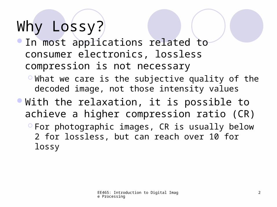
A Simple Experiment

Bit-plane representation

A=a0+a12+a222+ … … +a727

Least Significant Bit (LSB)

Most Significant Bit (MSB)

Example A=129 a0a1a2 …a7=10000001

a0a1a2 …a7=00110011 A=4+8+64+128=204


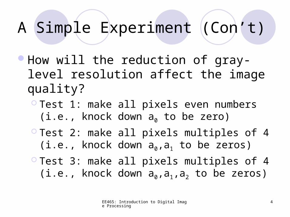
A Simple Experiment (Con’t)

How will the reduction of gray-level resolution affect the image quality? Test 1: make all pixels even numbers (i.e.,

knock down a0 to be zero) Test 2: make all pixels multiples of 4 (i.e., knock

down a0,a1 to be zeros) Test 3: make all pixels multiples of 4 (i.e., knock

down a0,a1,a2 to be zeros)


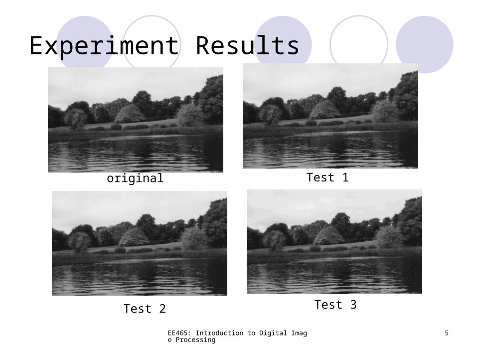
Experiment Results

original Test 1

Test 2 Test 3


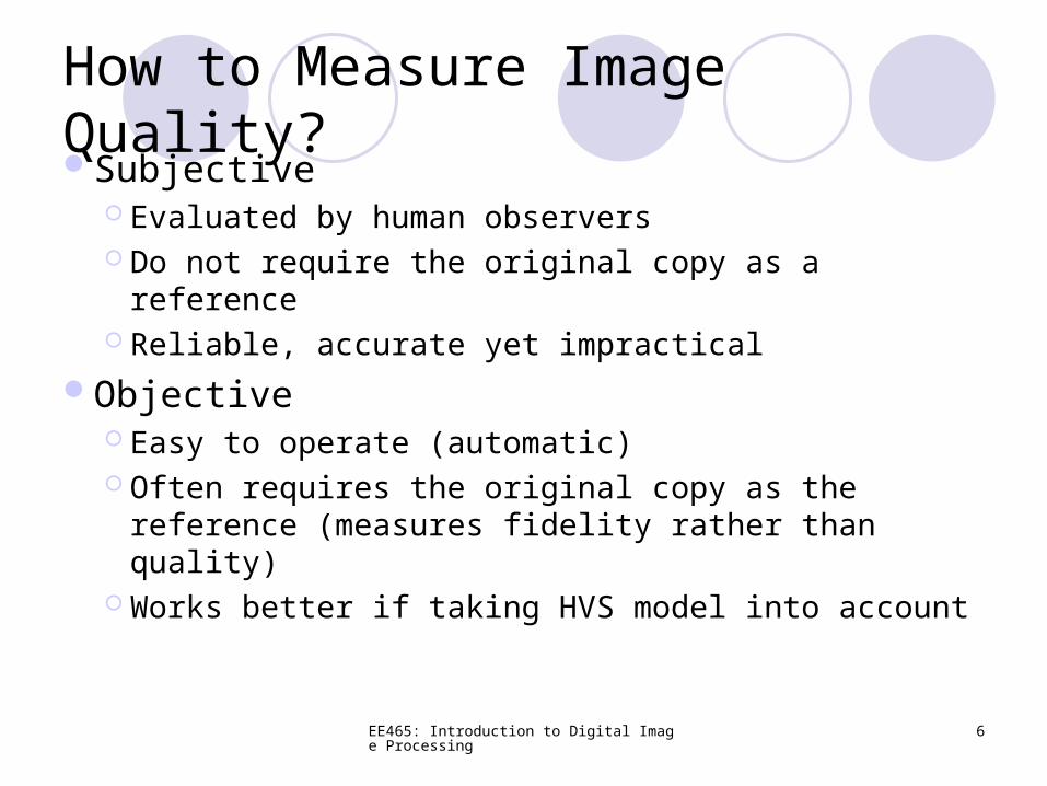
How to Measure Image Quality?Subjective

Evaluated by human observers Do not require the original copy as a reference Reliable, accurate yet impractical

Objective Easy to operate (automatic) Often requires the original copy as the

reference (measures fidelity rather than quality) Works better if taking HVS model into account


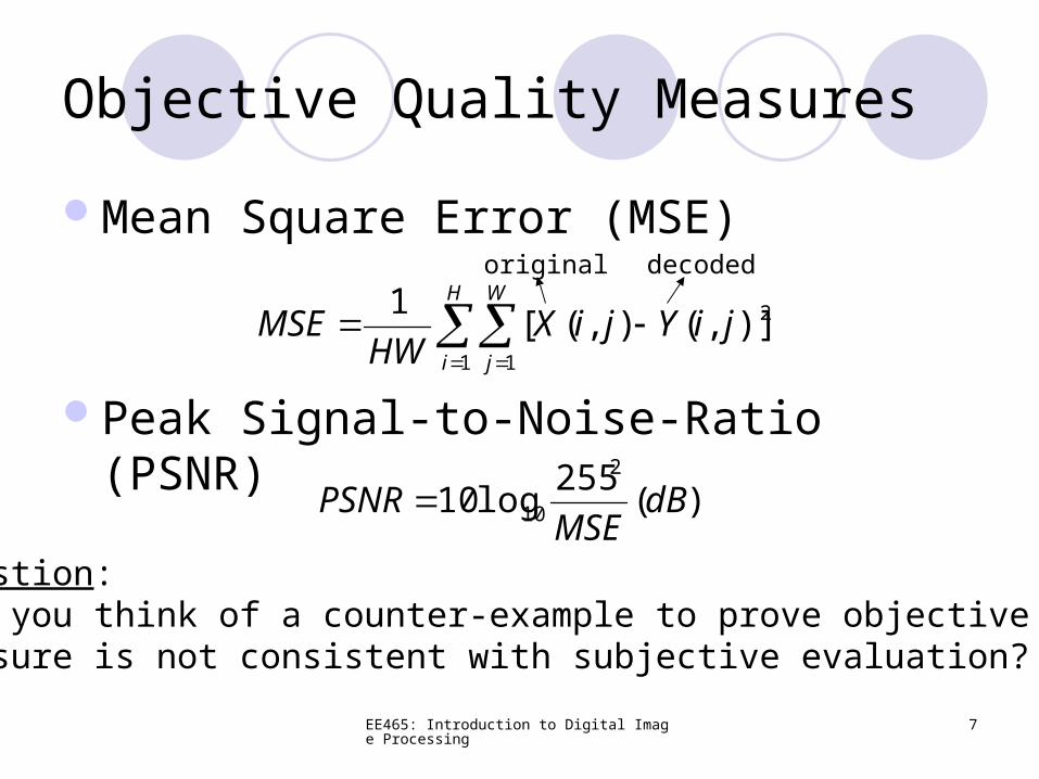
Mean Square Error (MSE)

Peak Signal-to-Noise-Ratio (PSNR)

H

i

W

j

jiYjiXHW

MSE1 1

2)],(),([1

)(255

log102

10 dBMSE

PSNR

Objective Quality Measures

original decoded

Question: Can you think of a counter-example to prove objective measure is not consistent with subjective evaluation?


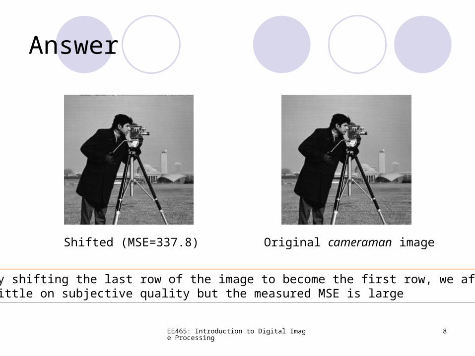
Answer

Shifted (MSE=337.8) Original cameraman image

By shifting the last row of the image to become the first row, we affectlittle on subjective quality but the measured MSE is large


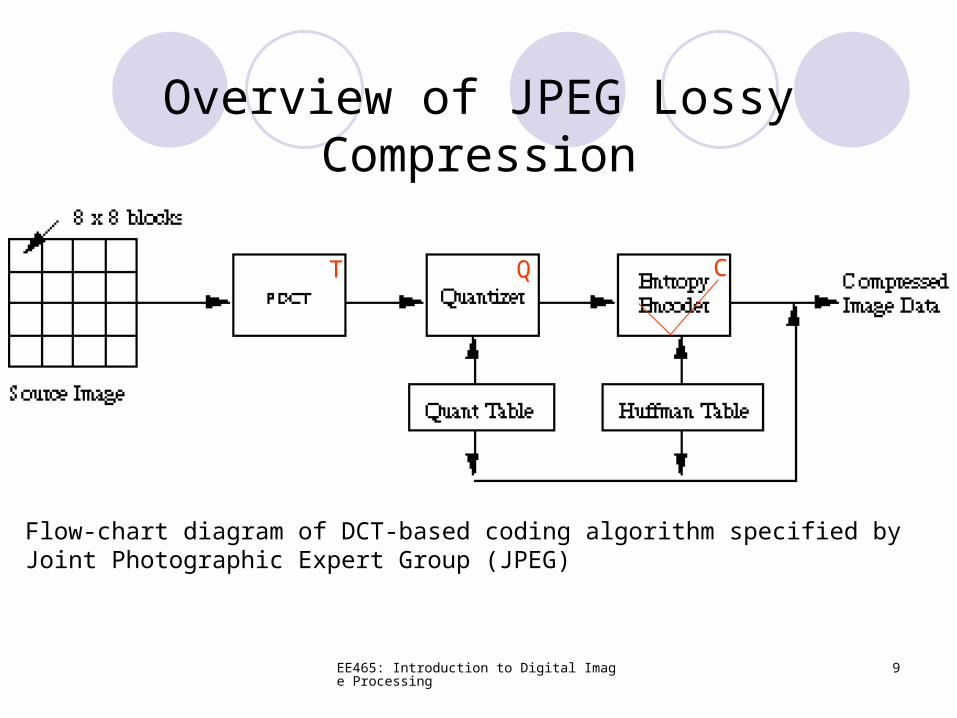
Overview of JPEG Lossy Compression

Flow-chart diagram of DCT-based coding algorithm specified by Joint Photographic Expert Group (JPEG)

T Q C


Lossy Image Compression:a Quick Tour of JPEG Coding Standard

Why lossy for grayscale images? Tradeoff between Rate and Distortion




and Huffman coding


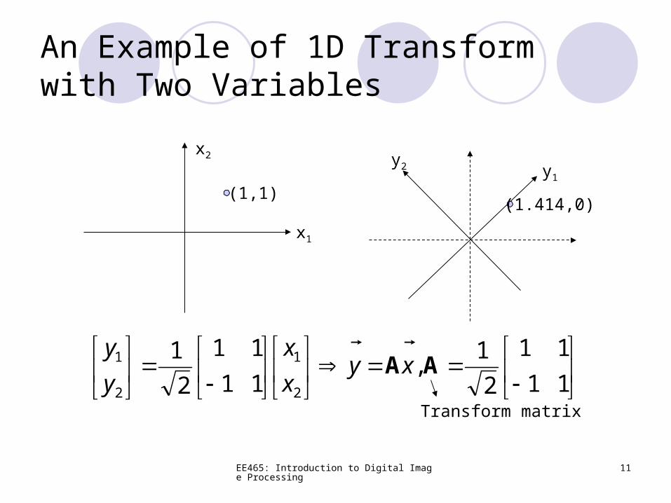
An Example of 1D Transform with Two Variables

x1

x2

y1

y2

11

11

2

1,

11

11

2

1

2

1

2

1 AAxyx

x

y

y

Transform matrix

(1,1)(1.414,0)


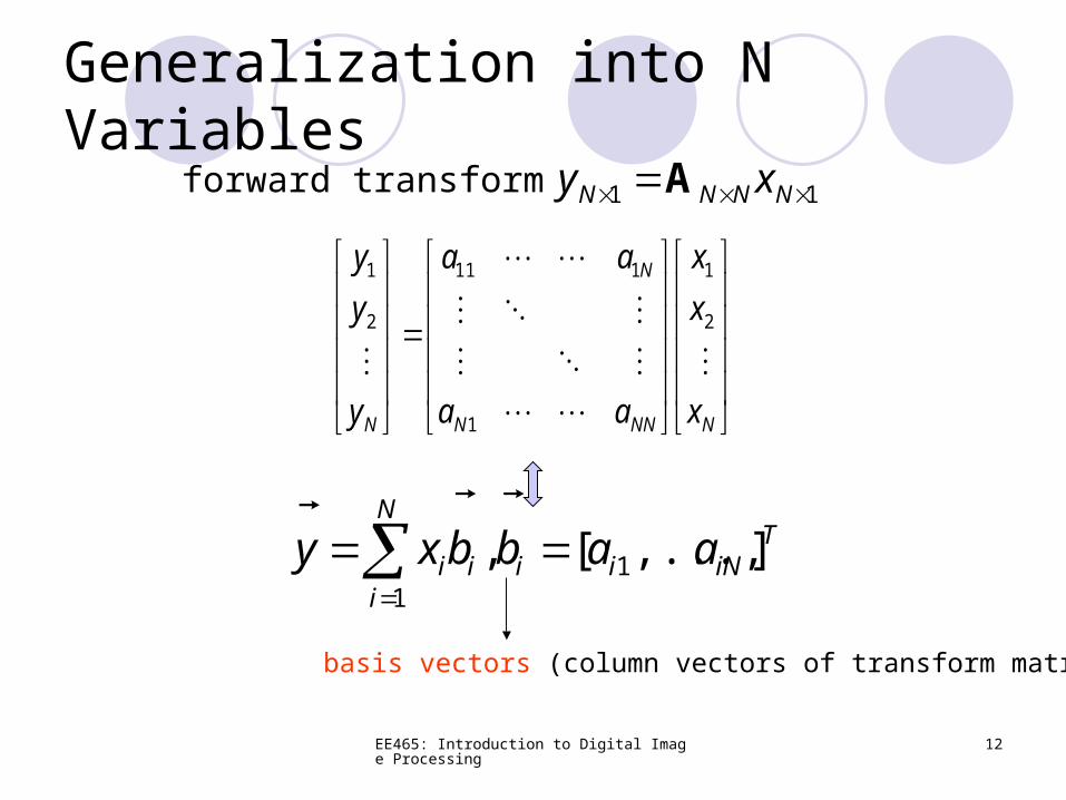
11 NNNN xy

Aforward transform

NNNN

N

N x

x

x

aa

aa

y

y

y

2

1

1

111

2

1

Generalization into N Variables

N

i

TiNiiii aabbxy

11 ],...,[,

basis vectors (column vectors of transform matrix)


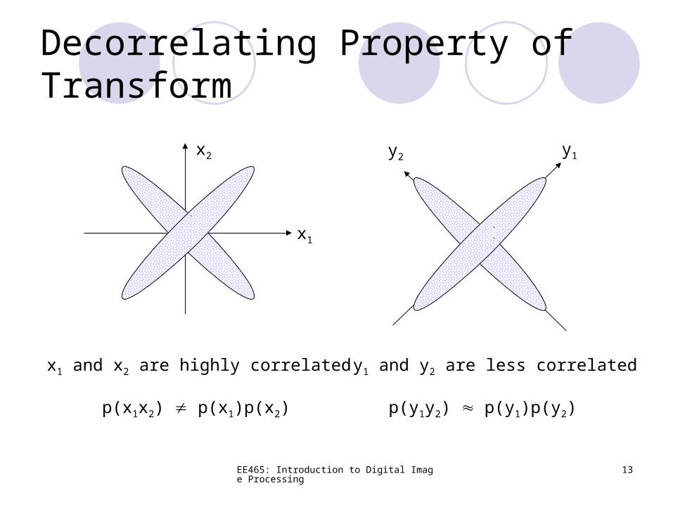
Decorrelating Property of Transform

x1

x2 y1y2

x1 and x2 are highly correlated

p(x1x2) p(x1)p(x2)

y1 and y2 are less correlated

p(y1y2) p(y1)p(y2)


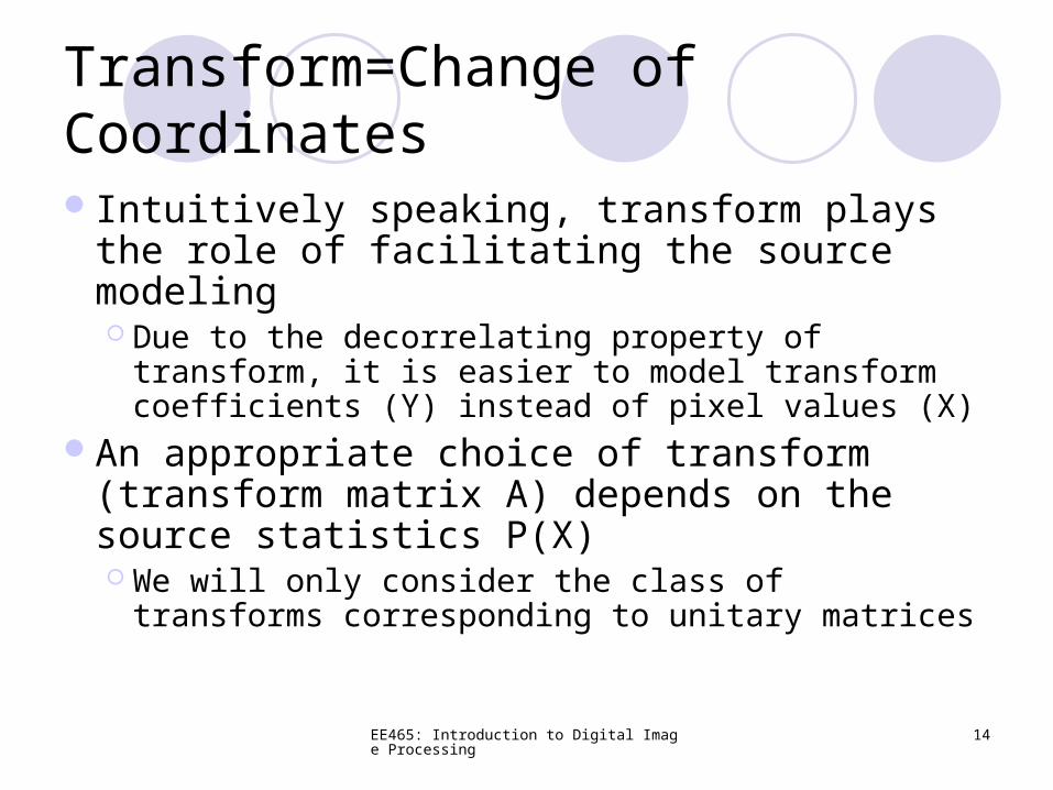
Transform=Change of CoordinatesIntuitively speaking, transform plays the

role of facilitating the source modeling Due to the decorrelating property of transform,

it is easier to model transform coefficients (Y) instead of pixel values (X)

An appropriate choice of transform (transform matrix A) depends on the source statistics P(X) We will only consider the class of transforms

corresponding to unitary matrices


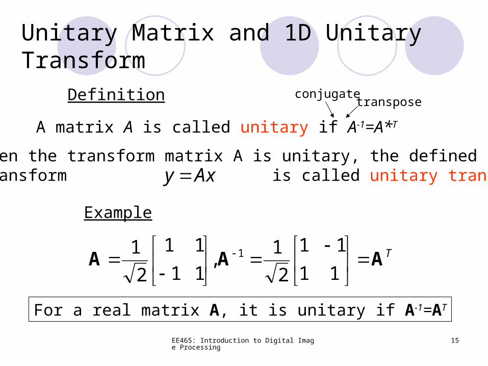
A matrix A is called unitary if A-1=A*T

Unitary Matrix and 1D Unitary Transform

Definition conjugatetranspose

When the transform matrix A is unitary, the defined transform is called unitary transform

Example

TAAA

11

11

2

1,

11

11

2

1 1

For a real matrix A, it is unitary if A-1=AT

xAy


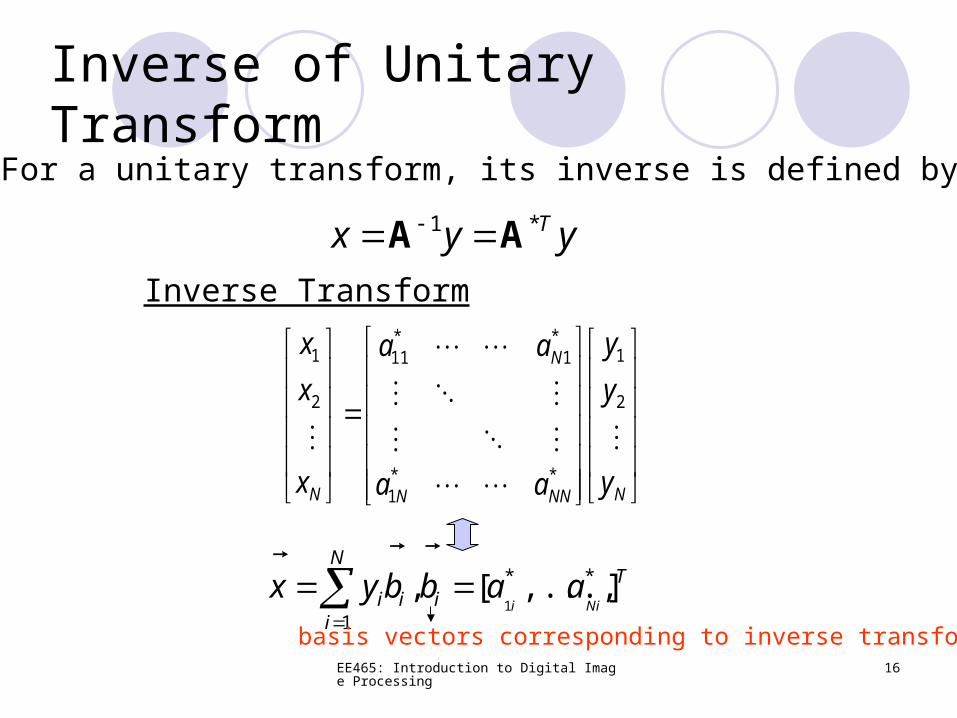
Inverse of Unitary TransformFor a unitary transform, its inverse is defined by

yyx T *1 AA

NNNN

N

N y

y

y

aa

aa

x

x

x

2

1

**1

*1

*11

2

1

Inverse Transform

N

i

Tiii Nii

aabbyx1

** ],...,[,1

basis vectors corresponding to inverse transform


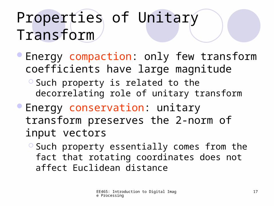
Properties of Unitary Transform

Energy compaction: only few transform coefficients have large magnitude Such property is related to the decorrelating

role of unitary transform

Energy conservation: unitary transform preserves the 2-norm of input vectors Such property essentially comes from the fact

that rotating coordinates does not affect Euclidean distance


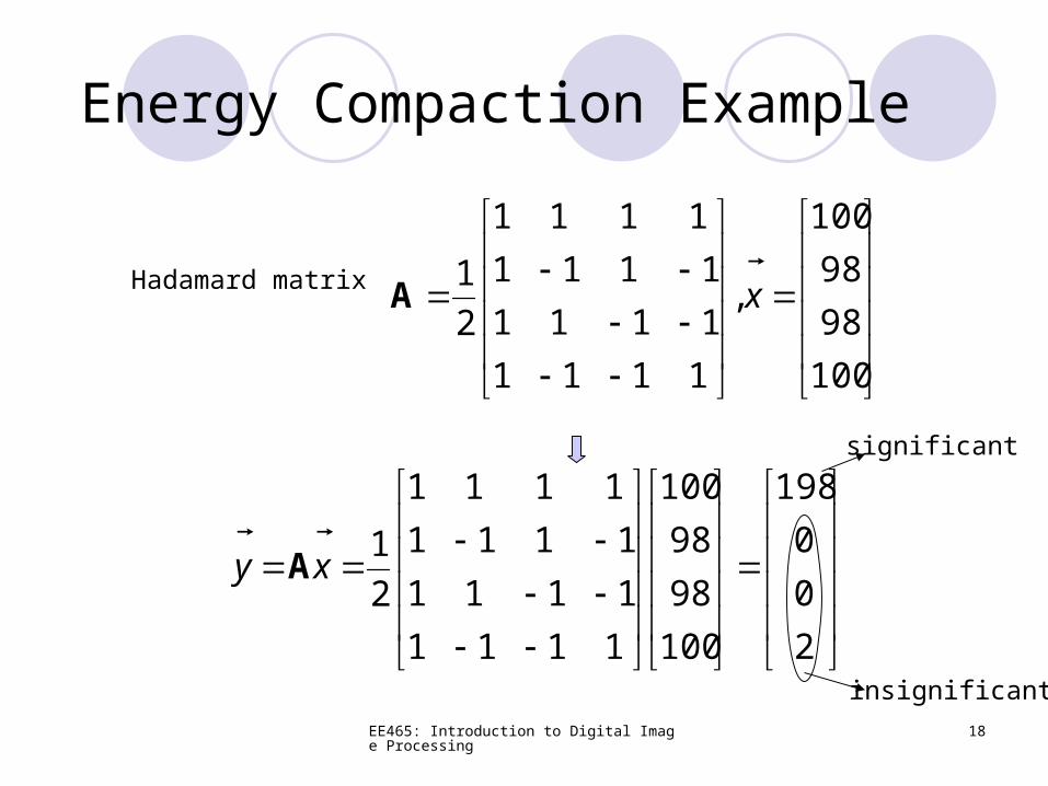
Energy Compaction Example

100

98

98

100

,

1111

1111

1111

1111

2

1x

AHadamard matrix

2

0

0

198

100

98

98

100

1111

1111

1111

1111

2

1xyA

insignificant

significant


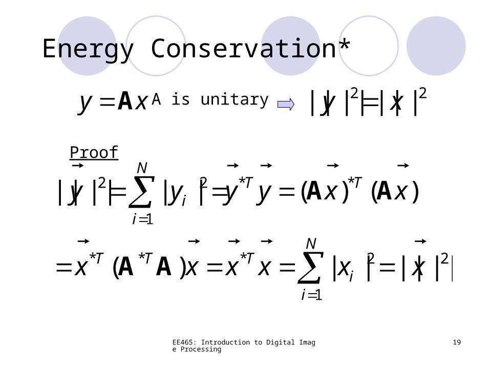
Energy Conservation*

xyA A is unitary 22 |||||||| xy

Proof

2

1

2***

**

1

22

||||||)(

)()(||||||

xxxxxx

xxyyyy

N

ii

TTT

TTN

ii

AA

AA


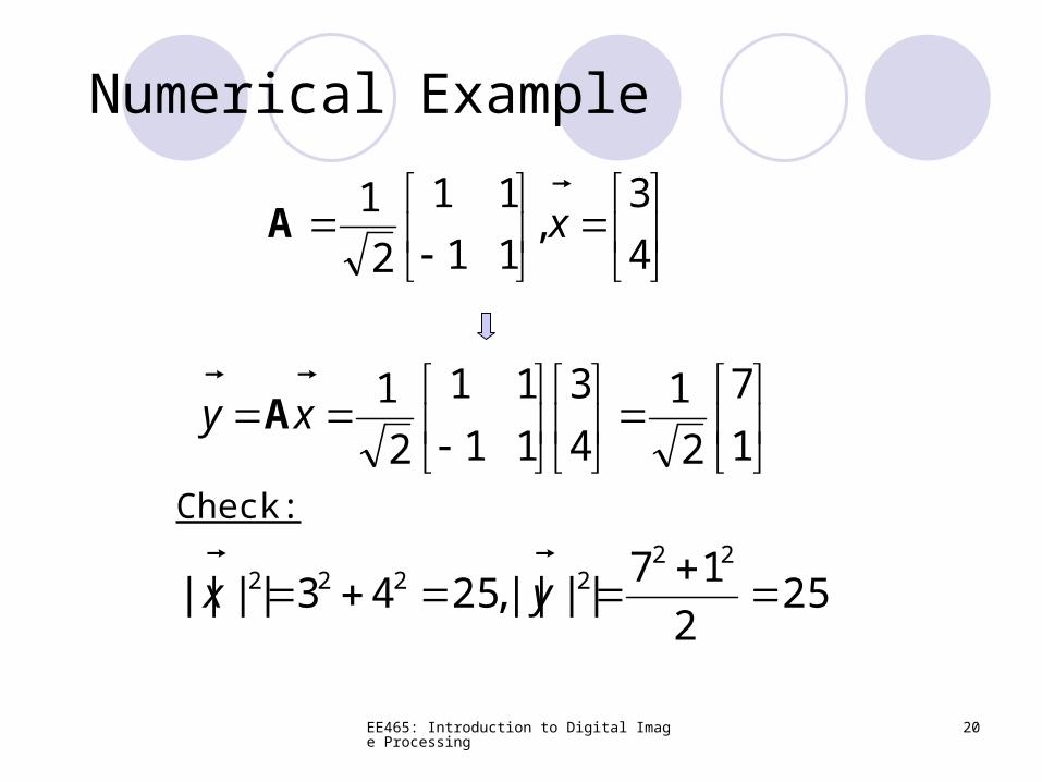
Numerical Example

4

3,

11

11

2

1x

A

1

7

2

1

4

3

11

11

2

1xyA

Check:

252

17||||,2543||||

222222

yx


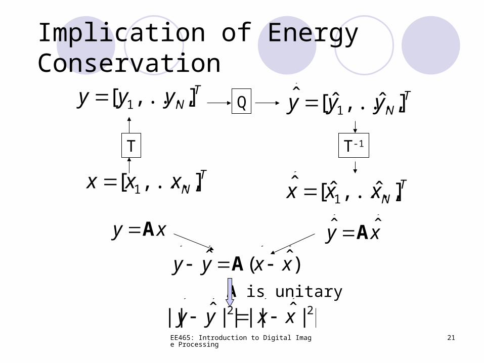
Implication of Energy Conservation

xyA

A is unitary

Q TNyyy ]ˆ,...,ˆ[ˆ

1T

Nyyy ],...,[ 1

TNxxx ],...,[ 1

T T-1

TNxxx ]ˆ,...,ˆ[ˆ

1

xy ˆˆ A

)ˆ(ˆ xxyy

A

22 ||ˆ||||ˆ|| xxyy


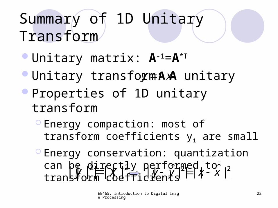
Summary of 1D Unitary TransformUnitary matrix: A-1=A*T

Unitary transform: A unitaryProperties of 1D unitary transform

Energy compaction: most of transform coefficients yi are small

Energy conservation: quantization can be directly performed to transform coefficients

xyA

22 |||||||| xy

22 ||ˆ||||ˆ|| xxyy


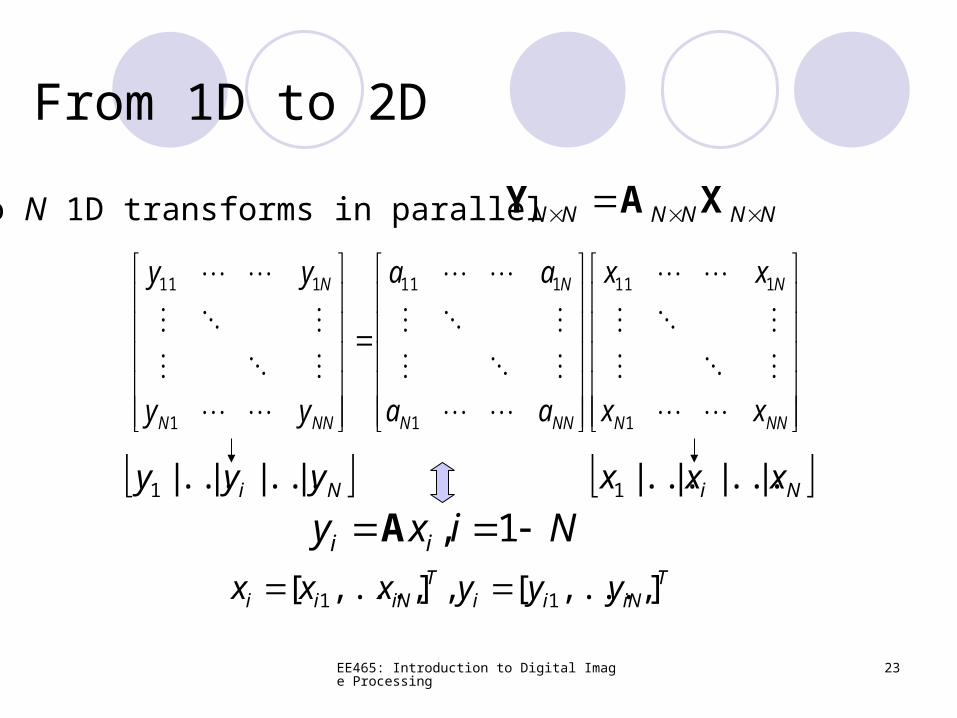
NNNNNN XAYDo N 1D transforms in parallel

NNN

N

NNN

N

NNN

N

xx

xx

aa

aa

yy

yy

1

111

1

111

1

111

From 1D to 2D

Nixy ii 1,A

TiNii

TiNii yyyxxx ],...,[,],...,[ 11

Ni yyy

|...||...|1 Ni xxx

|...||...|1


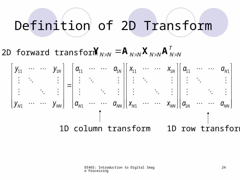
TNNNNNNNN AXAY2D forward transform

NNN

N

NNN

N

NNN

N

NNN

N

aa

aa

xx

xx

aa

aa

yy

yy

1

111

1

111

1

111

1

111

1D column transform 1D row transform

Definition of 2D Transform


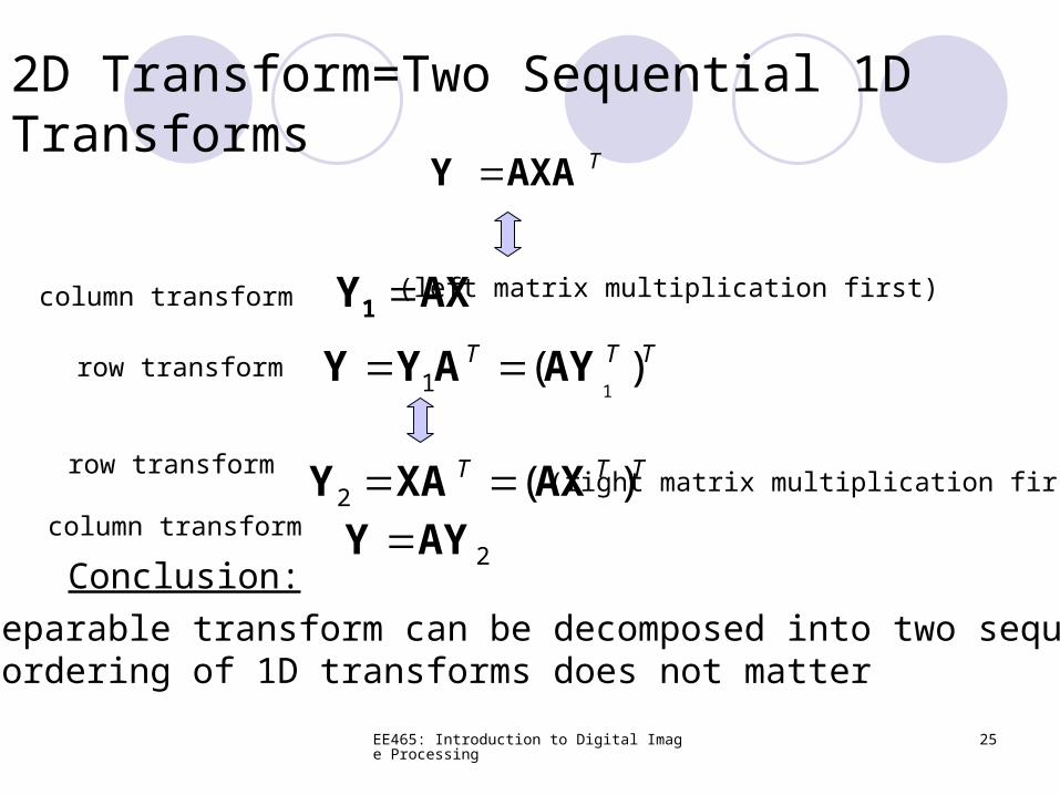
2D Transform=Two Sequential 1D Transforms

Conclusion:

2D separable transform can be decomposed into two sequential The ordering of 1D transforms does not matter

TAXAY

AXY1 TTT )(

11 AYAYY row transform

column transform

TTT )(2 AXXAY

2AYY

row transform

column transform

(left matrix multiplication first)

(right matrix multiplication first)


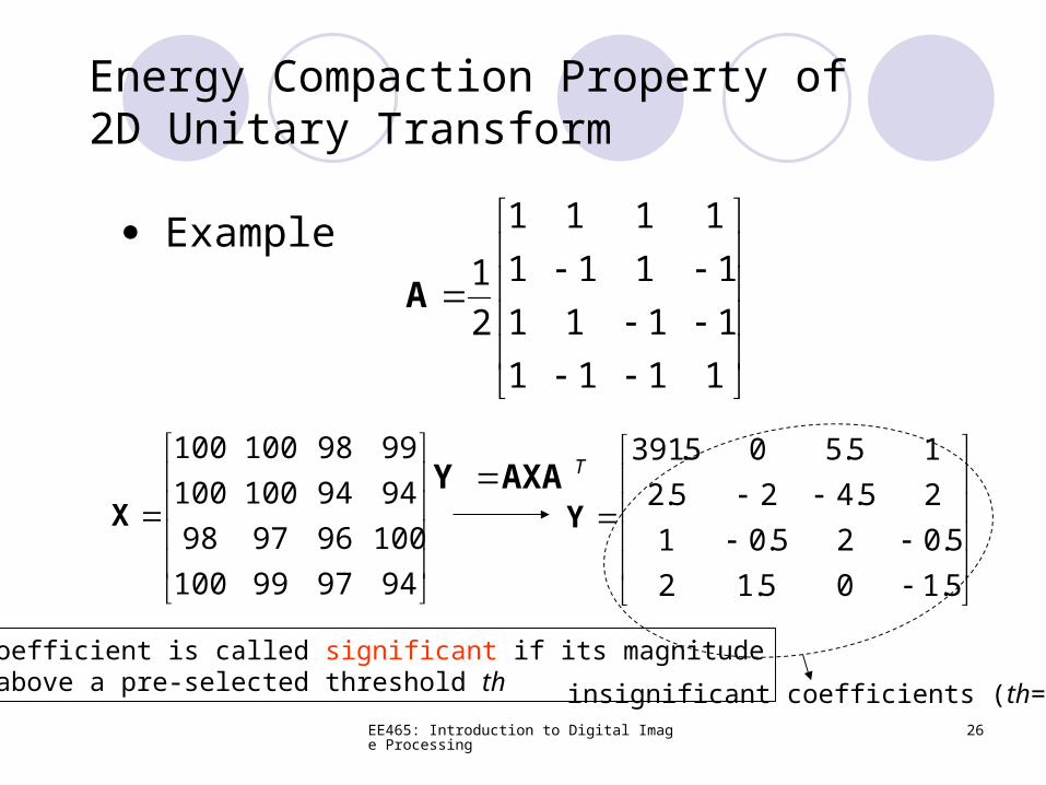
Energy Compaction Property of 2D Unitary Transform

Example

949799100

100969798

9494100100

9998100100

X

5.105.12

5.025.01

25.425.2

15.505.391

Y

TAXAY

1111

1111

1111

1111

2

1A

insignificant coefficients (th=64)

A coefficient is called significant if its magnitudeis above a pre-selected threshold th


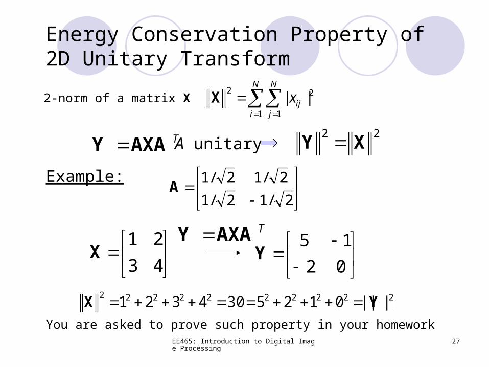
Energy Conservation Property of 2D Unitary Transform

TAXAY 22

XY

Example:

2/12/1

2/12/1A

43

21X

02

15Y

TAXAY

2222222222||||0125304321 YX

2-norm of a matrix X

N

i

N

jijx

1 1

22||X

A unitary

You are asked to prove such property in your homework


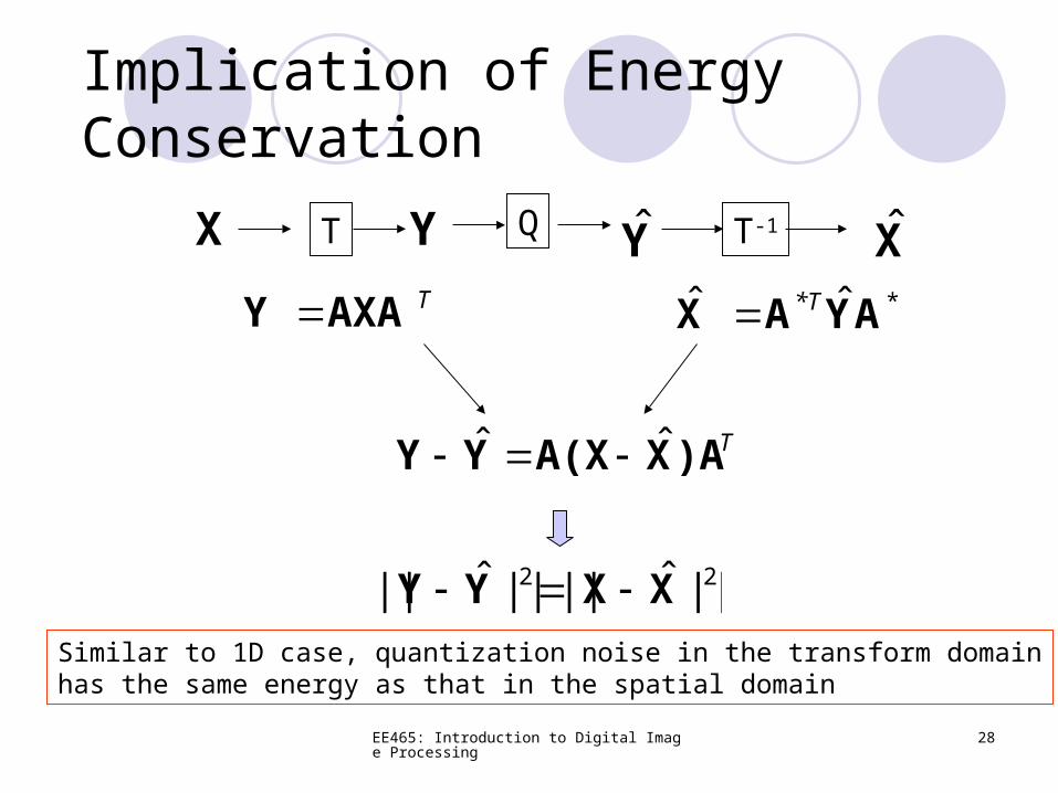
TAXAY *ˆˆ AYAX *T

T)AXA(XYY ˆˆ

22 ||ˆ||||ˆ|| XXYY

Implication of Energy Conservation

Q YYX T T-1 X

Similar to 1D case, quantization noise in the transform domainhas the same energy as that in the spatial domain


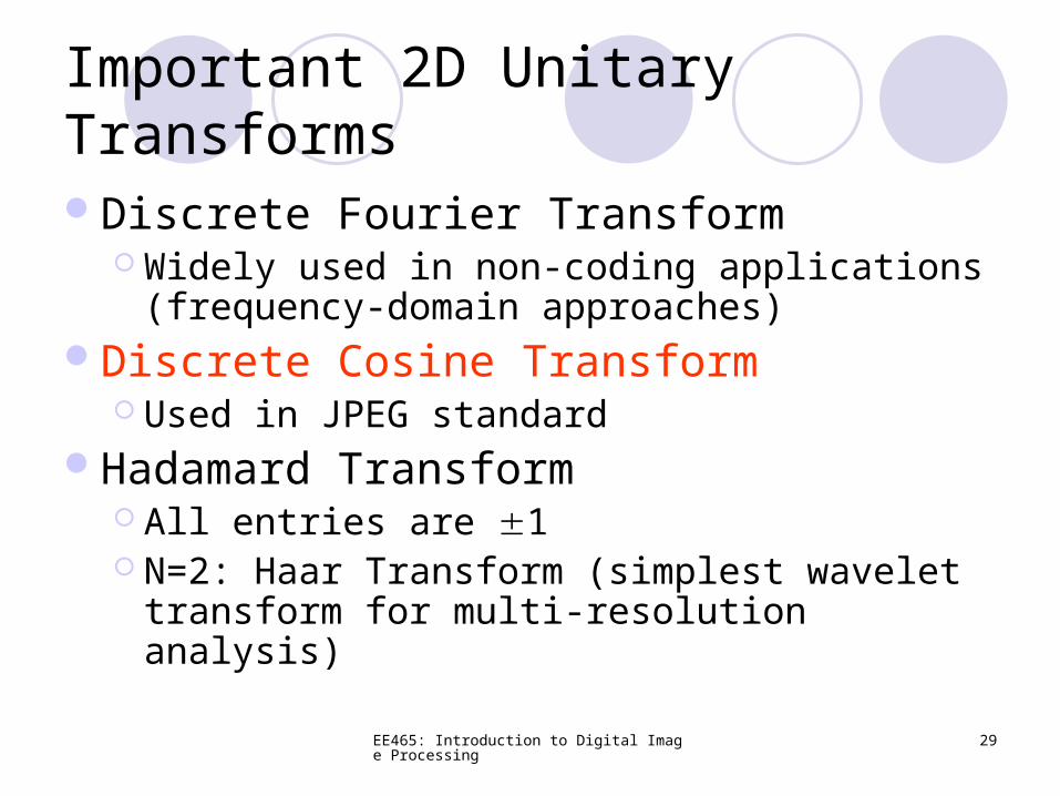
Important 2D Unitary Transforms

Discrete Fourier Transform Widely used in non-coding applications

(frequency-domain approaches)Discrete Cosine Transform

Used in JPEG standardHadamard Transform

All entries are 1 N=2: Haar Transform (simplest wavelet

transform for multi-resolution analysis)


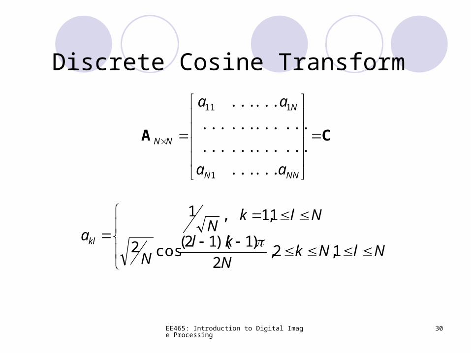
Discrete Cosine Transform

CA

NNN

N

NN

aa

aa

......

............

............

......

1

111

NlNkN

klN

NlkN

akl1,2,

2

)1)(12(cos2

1,1,1


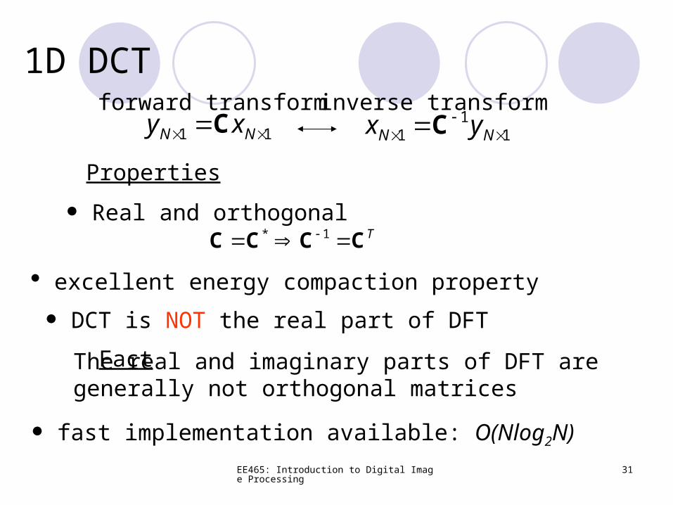
11 NN xyC 1

11

NN yx

C

forward transform inverse transform

1D DCT

Real and orthogonalTCCCC 1*

fast implementation available: O(Nlog2N)

excellent energy compaction property

DCT is NOT the real part of DFT

Fact The real and imaginary parts of DFT are generally not orthogonal matrices

Properties


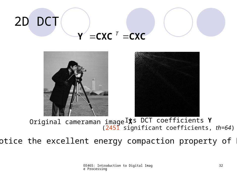
2D DCTCXCCXCY T

Notice the excellent energy compaction property of DCT

Original cameraman image X Its DCT coefficients Y(2451 significant coefficients, th=64)


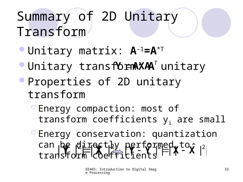
Summary of 2D Unitary TransformUnitary matrix: A-1=A*T

Unitary transform: A unitaryProperties of 2D unitary transform

Energy compaction: most of transform coefficients yi are small

Energy conservation: quantization can be directly performed to transform coefficients

TAXAY

22 |||||||| XY 22 ||ˆ||||ˆ|| XXYY







and Huffman coding


What is Quantization?

In Physics To limit the possible values of a magnitude or

quantity to a discrete set of values by quantum mechanical rules

In image compression To limit the possible values of a pixel value or a

transform coefficient to a discrete set of values by information theoretic rules


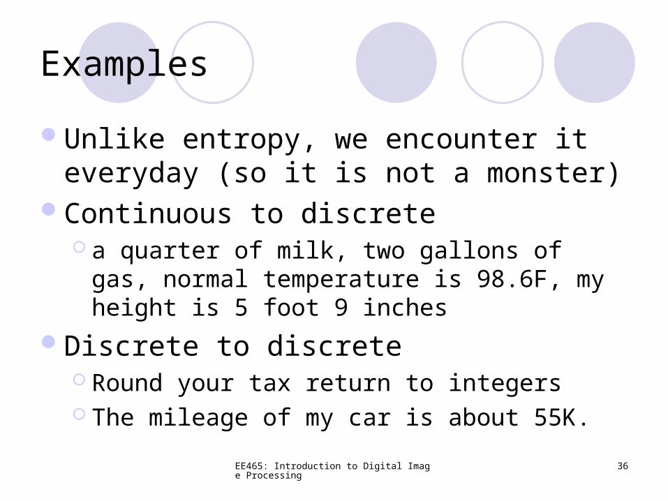
Examples

Unlike entropy, we encounter it everyday (so it is not a monster)

Continuous to discrete a quarter of milk, two gallons of gas, normal

temperature is 98.6F, my height is 5 foot 9 inches

Discrete to discrete Round your tax return to integers The mileage of my car is about 55K.


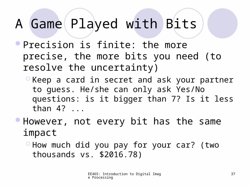
A Game Played with BitsPrecision is finite: the more precise, the

more bits you need (to resolve the uncertainty) Keep a card in secret and ask your partner to

guess. He/she can only ask Yes/No questions: is it bigger than 7? Is it less than 4? ...

However, not every bit has the same impact How much did you pay for your car? (two

thousands vs. $2016.78)


Scalar vs. Vector Quantization

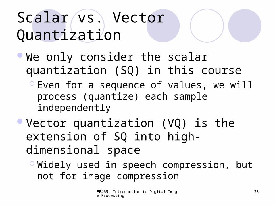
We only consider the scalar quantization (SQ) in this course Even for a sequence of values, we will process

(quantize) each sample independently

Vector quantization (VQ) is the extension of SQ into high-dimensional space Widely used in speech compression, but not for

image compression


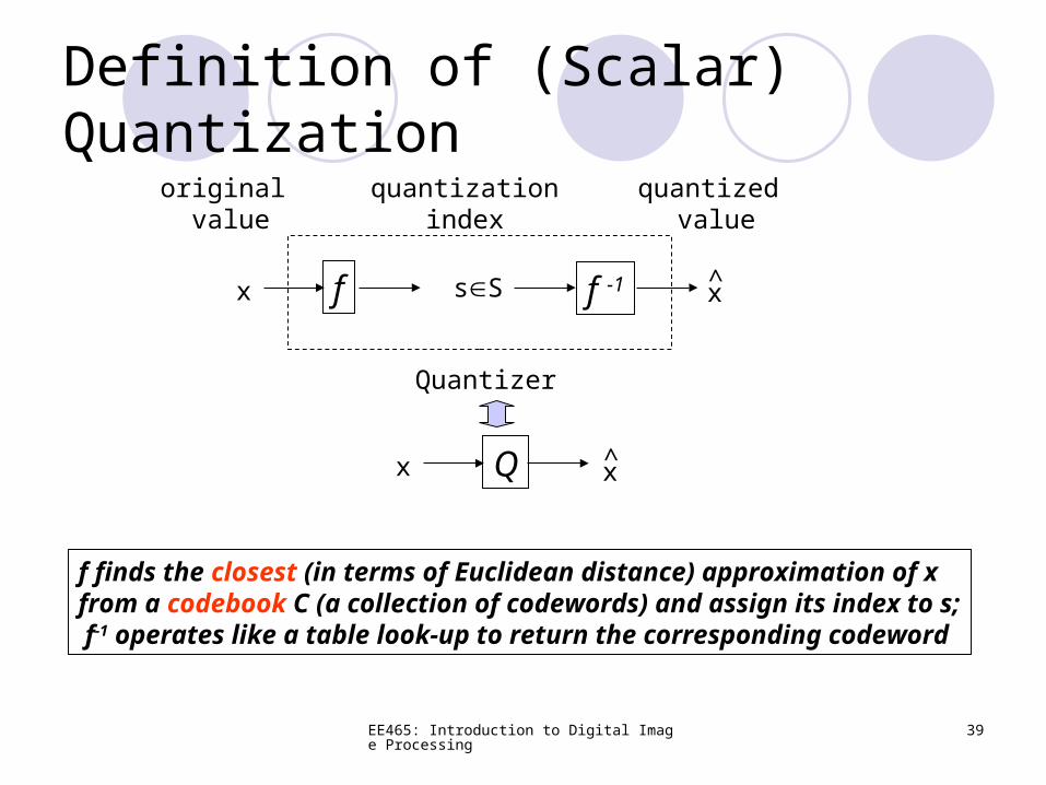
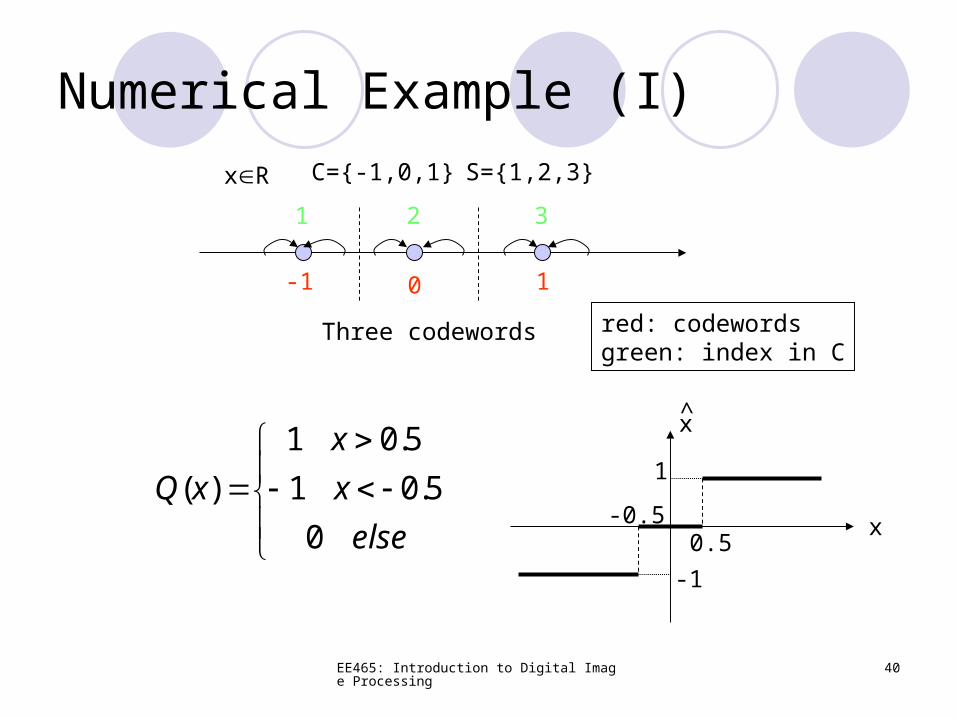
Definition of (Scalar) Quantization

x f f -1 xsS

original value

quantizationindex

quantized value

Quantizer

x Q x

f finds the closest (in terms of Euclidean distance) approximation of x from a codebook C (a collection of codewords) and assign its index to s; f-1 operates like a table look-up to return the corresponding codeword


Numerical Example (I)

0 1-1

C={-1,0,1}

Three codewords

else

x

x

xQ

0

5.01

5.01

)(

S={1,2,3}

1 2 3

red: codewordsgreen: index in C

x

x

0.5-0.5

1

-1

xR


Numerical Example (II)

24 408

C={8,24,40,56,72,…,248}

sixteen codewords

]255,0[,1616

8)(

x

xxQ

S={1,2,3,…,16}

1 2 3

red: codewordsgreen: index in C

x

x

...

...

248

16

x{0,1,…,255}

16 32

24

40

(note that the scales are different)

8floor operation


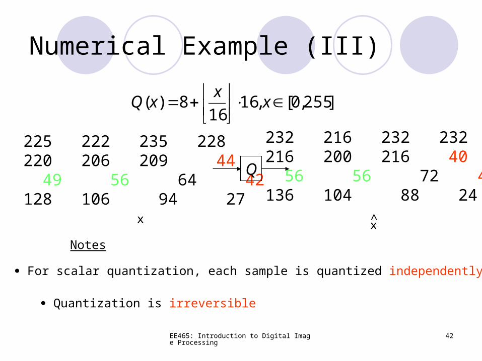
Numerical Example (III)

225 222 235 228 220 206 209 44 49 56 64 42 128 106 94 27

Q

xx

]255,0[,1616

8)(

x

xxQ

232 216 232 232 216 200 216 40 56 56 72 40 136 104 88 24

For scalar quantization, each sample is quantized independently

Notes

Quantization is irreversible


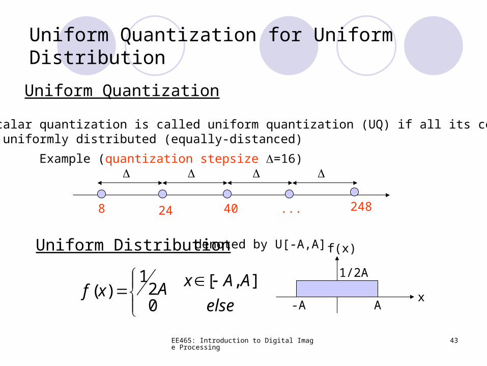
Uniform Quantization for Uniform Distribution

Uniform Quantization

A scalar quantization is called uniform quantization (UQ) if all its codewords are uniformly distributed (equally-distanced)

24 408 ... 248

Example (quantization stepsize =16)

Uniform Distribution

else

AAxAxf0

],[21

)(-A A

1/2A

x

f(x)denoted by U[-A,A]


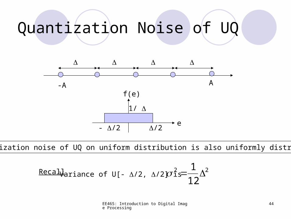
Quantization Noise of UQ

- /2 /2

1/

e

f(e)

Quantization noise of UQ on uniform distribution is also uniformly distributed

Recall 22

12

1Variance of U[- /2, /2] is

-A A


6dB/bit Rule

222

3

1)2(

12

1AAs Signal: X ~ U[-A,A]

22

12

1eNoise: e ~ U[- /2, /2]

N

A2

Choose N=2n (n-bit)codewords for X

)(02.6log20

12

3log10log10 102

2

102

2

10 dBnN

A

SNRe

s

N=2n

(quantization stepsize)







and Huffman coding


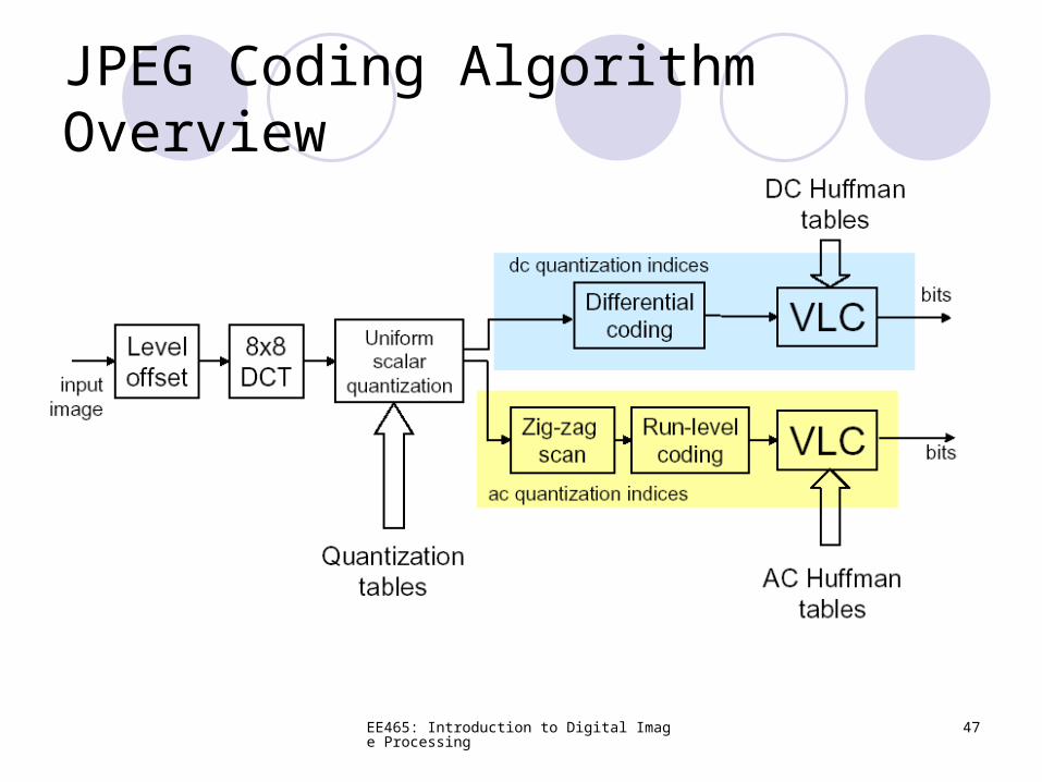
JPEG Coding Algorithm Overview


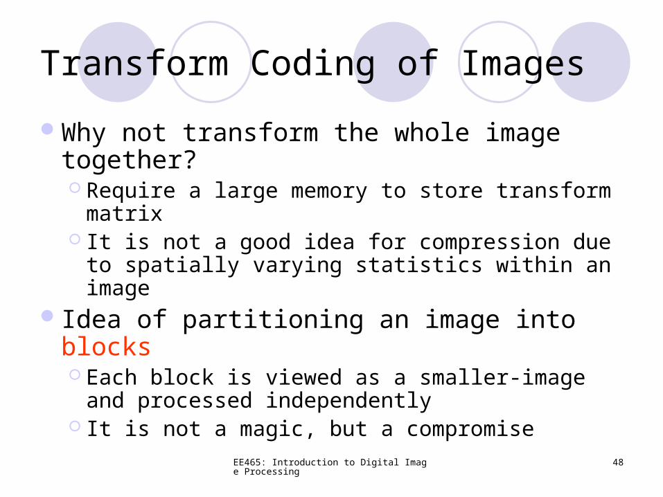
Transform Coding of Images

Why not transform the whole image together? Require a large memory to store transform

matrix It is not a good idea for compression due to

spatially varying statistics within an imageIdea of partitioning an image into blocks

Each block is viewed as a smaller-image and processed independently

It is not a magic, but a compromise


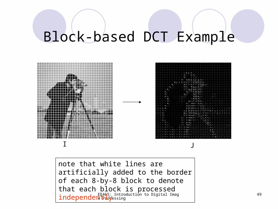
Block-based DCT Example

JI

note that white lines are artificially added to the border of each 8-by-8 block to denote that each block is processed independently


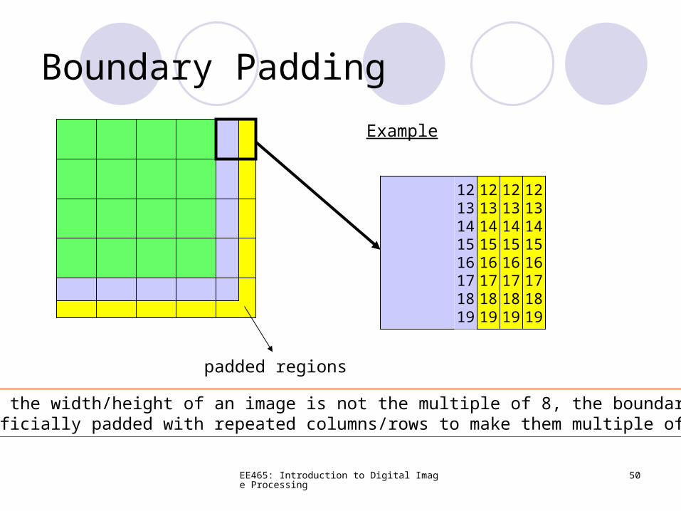
Boundary Padding

padded regions

Example

1213141516171819

1213141516171819

1213141516171819

1213141516171819

When the width/height of an image is not the multiple of 8, the boundary isartificially padded with repeated columns/rows to make them multiple of 8


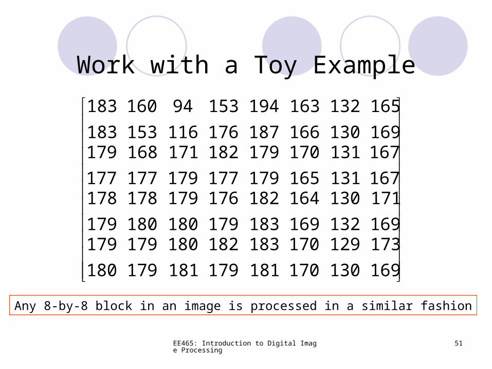
Work with a Toy Example

169130

173129

170181

170183

179181

182180

179180

179179169132

171130

169183

164182

179180

176179

180179

178178167131

167131

165179

170179

177179

182171

177177

168179169130

165132

166187

163194

176116

15394

153183

160183

Any 8-by-8 block in an image is processed in a similar fashion


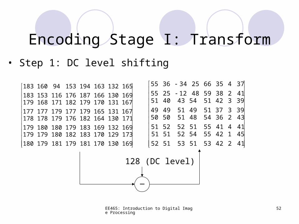
Encoding Stage I: Transform

• Step 1: DC level shifting

169130

173129

170181

170183

179181

182180

179180

179179169132

171130

169183

164182

179180

176179

180179

178178167131

167131

165179

170179

177179

182171

177177

168179169130

165132

166187

163194

176116

15394

153183

160183

412

451

4253

4255

5153

5452

5152

5151414

432

4155

3654

5152

4851

5251

5050393

393

3751

4251

4951

5443

4949

4051412

374

3859

3566

4812

2534

2555

3655

128 (DC level)

_


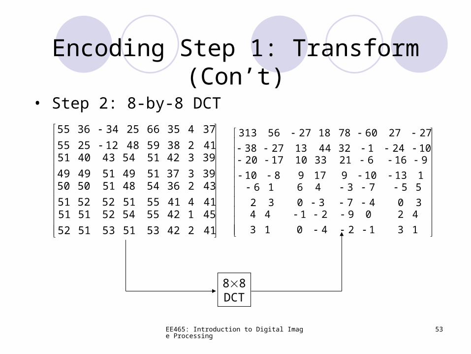
• Step 2: 8-by-8 DCT

412

451

4253

4255

5153

5452

5152

5151414

432

4155

3654

5152

4851

5251

5050393

393

3751

4251

4951

5443

4949

4051412

374

3859

3566

4812

2534

2555

3655

13

42

12

09

40

21

13

4430

55

47

73

30

46

32

16113

916

109

621

179

3310

810

17201024

2727

132

6078

4413

1827

2738

56313

Encoding Step 1: Transform (Con’t)

88DCT


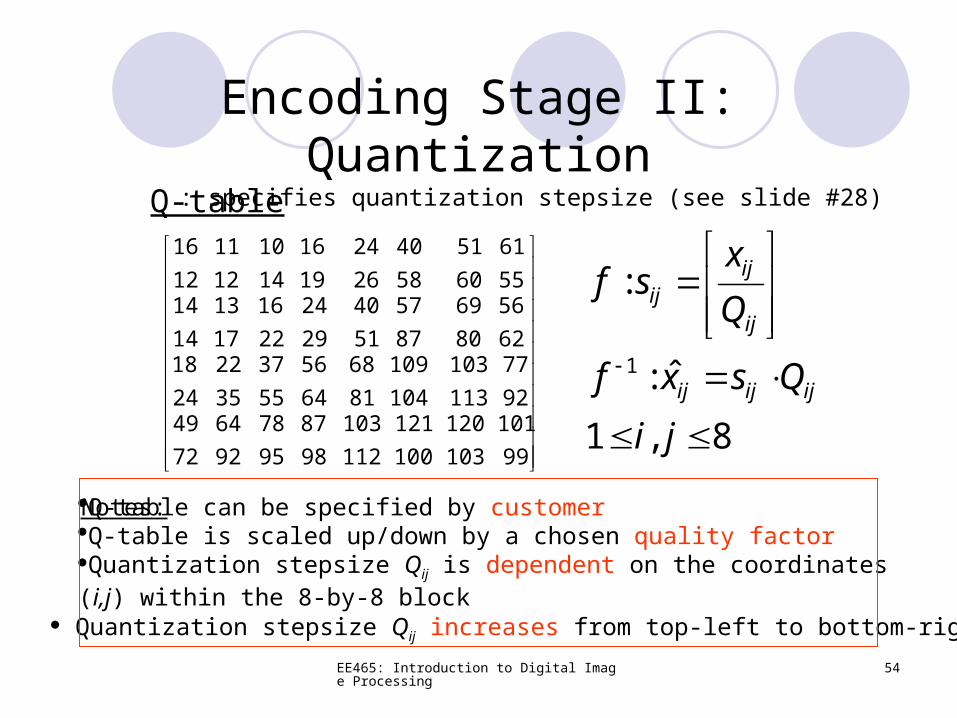
Encoding Stage II: Quantization

99103

101120

100112

121103

9895

8778

9272

644992113

77103

10481

10968

6455

5637

3524

22186280

5669

8751

5740

2922

2416

1714

13145560

6151

5826

4024

1914

1610

1212

1116

Q-table

8,1

ˆ:

:

1

ji

Qsxf

Q

xsf

ijijij

ij

ijij

: specifies quantization stepsize (see slide #28)

Notes: Q-table can be specified by customerQ-table is scaled up/down by a chosen quality factor Quantization stepsize Qij is dependent on the coordinates (i,j) within the 8-by-8 block Quantization stepsize Qij increases from top-left to bottom-right


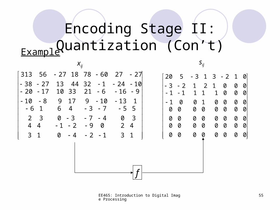
Encoding Stage II: Quantization (Con’t)

13

42

12

09

40

21

13

4430

55

47

73

30

46

32

16113

916

109

621

179

3310

810

17201024

2727

132

6078

4413

1827

2738

56313

00

00

00

00

00

00

00

0000

00

00

00

00

00

00

0000

00

00

01

10

11

01

1100

01

01

23

21

13

23

520

Example

f

xijsij


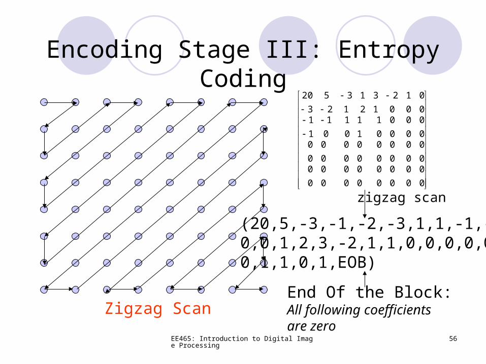
Encoding Stage III: Entropy Coding

Zigzag Scan

00

00

00

00

00

00

00

0000

00

00

00

00

00

00

0000

00

00

01

10

11

01

1100

01

01

23

21

13

23

520

(20,5,-3,-1,-2,-3,1,1,-1,-1,0,0,1,2,3,-2,1,1,0,0,0,0,0,0,1,1,0,1,EOB)

zigzag scan

End Of the Block:All following coefficients are zero


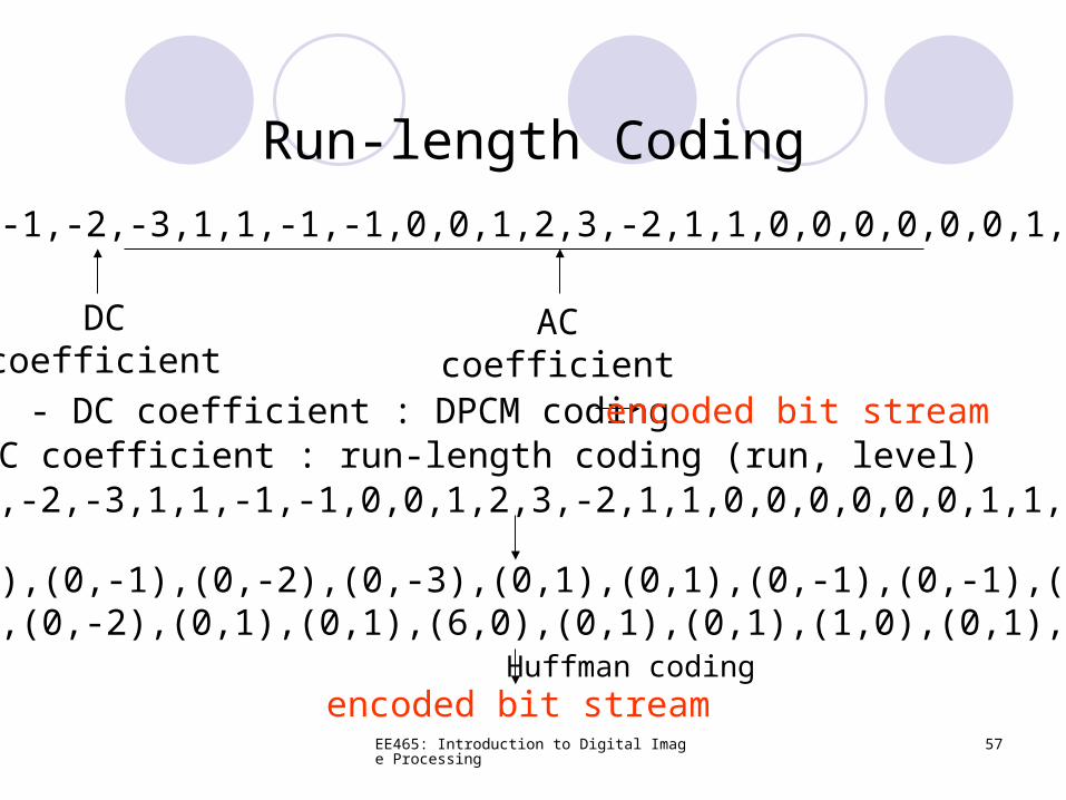
Run-length Coding

(20,5,-3,-1,-2,-3,1,1,-1,-1,0,0,1,2,3,-2,1,1,0,0,0,0,0,0,1,1,0,1,EOB)

DCcoefficient

ACcoefficient

- DC coefficient : DPCM coding- AC coefficient : run-length coding (run, level)

(5,-3,-1,-2,-3,1,1,-1,-1,0,0,1,2,3,-2,1,1,0,0,0,0,0,0,1,1,0,1,EOB)

(0,5),(0,-3),(0,-1),(0,-2),(0,-3),(0,1),(0,1),(0,-1),(0,-1),(2,0),(0,1),(0,2),(0,3),(0,-2),(0,1),(0,1),(6,0),(0,1),(0,1),(1,0),(0,1),EOB

Huffman codingencoded bit stream

encoded bit stream


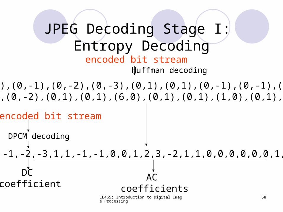
JPEG Decoding Stage I: Entropy Decoding

(20,5,-3,-1,-2,-3,1,1,-1,-1,0,0,1,2,3,-2,1,1,0,0,0,0,0,0,1,1,0,1,EOB)

Huffman decodingencoded bit stream

AC coefficients

DC coefficient

DPCM decoding

(0,5),(0,-3),(0,-1),(0,-2),(0,-3),(0,1),(0,1),(0,-1),(0,-1),(2,0),(0,1),(0,2),(0,3),(0,-2),(0,1),(0,1),(6,0),(0,1),(0,1),(1,0),(0,1),EOB

encoded bit stream


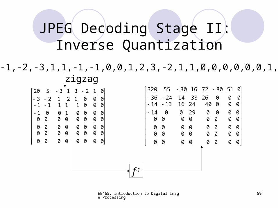
JPEG Decoding Stage II: Inverse Quantization

(20,5,-3,-1,-2,-3,1,1,-1,-1,0,0,1,2,3,-2,1,1,0,0,0,0,0,0,1,1,0,1,EOB)

00

00

00

00

00

00

00

0000

00

00

00

00

00

00

0000

00

00

01

10

11

01

1100

01

01

23

21

13

23

520

zigzag

00

00

00

00

00

00

00

0000

00

00

00

00

00

00

0000

00

00

040

290

2416

014

131400

051

026

8072

3814

1630

2436

55320

f-1


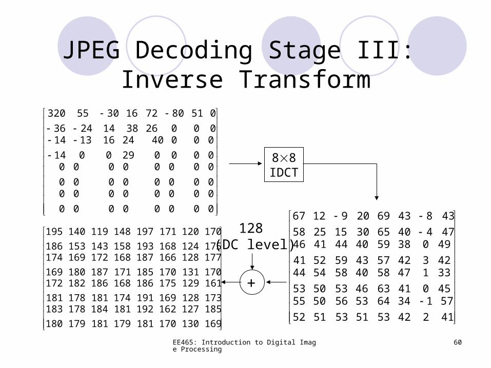
JPEG Decoding Stage III: Inverse Transform

00

00

00

00

00

00

00

0000

00

00

00

00

00

00

0000

00

00

040

290

2416

014

131400

051

026

8072

3814

1630

2436

55320

169130

185127

170181

162192

179181

181184

179180

178183173128

161129

169191

175186

174181

168186

178181

182172170131

177128

170185

166187

171187

168172

180169

169174175124

170120

168193

171197

158143

148119

153186

140195

412

571

4253

3464

5153

5356

5152

5055450

331

4163

4758

4653

4058

5053

5444423

490

4257

3859

4359

4044

5241

4146474

438

4065

4369

3015

209

2558

1267

88IDCT

128 (DC level)

+


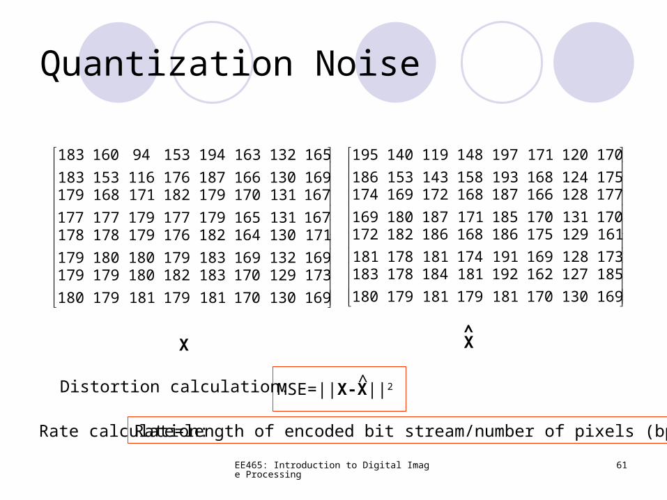
Quantization Noise

169130

173129

170181

170183

179181

182180

179180

179179169132

171130

169183

164182

179180

176179

180179

178178167131

167131

165179

170179

177179

182171

177177

168179169130

165132

166187

163194

176116

15394

153183

160183

169130

185127

170181

162192

179181

181184

179180

178183173128

161129

169191

175186

174181

168186

178181

182172170131

177128

170185

166187

171187

168172

180169

169174175124

170120

168193

171197

158143

148119

153186

140195

X X^

MSE=||X-X||2^Distortion calculation:

Rate calculation: Rate=length of encoded bit stream/number of pixels (bps)


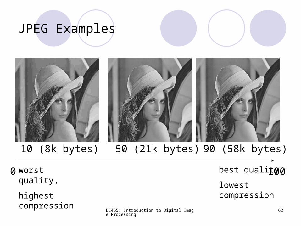
JPEG Examples

1000

90 (58k bytes)50 (21k bytes)10 (8k bytes)

best quality,

lowest compression

worst quality,

highest compression


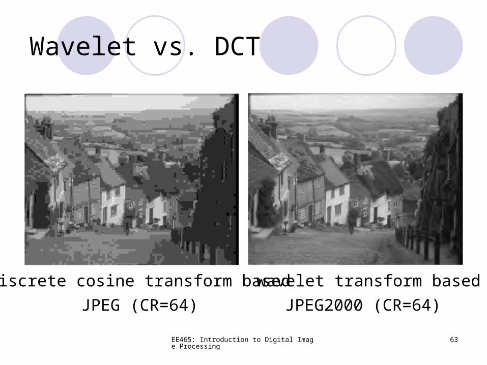
Wavelet vs. DCT

JPEG (CR=64) JPEG2000 (CR=64)

discrete cosine transform based wavelet transform based


Image Compression Summary

JPEG=T+Q+C (so is JPEG2000 except T becomes wavelet transform instead of DCT)

Key idea: sparsity of transform coefficients (most transform coefficients are quantized to zero)

Main weakness: blocky artifacts at low bit rates (many deblocking algorithms have been proposed in the literature)


One-Minute Survey

How much do you think you have understood today’s lecture? A) >90%, B)70-90%, C)50-70%, D) <50%

How long have you spent on final project so far?

What is the best score you have reached so far? (please indicate your status: G/UG)

Documents

Lossy Image Compression: a Quick Tour of JPEG Coding Standard