Embed Size (px)
Citation preview
LOTUS?: Algorithm Specifications and Supporting
Documentation
Le Trieu Phong1, Takuya Hayashi1,2, Yoshinori Aono1, Shiho Moriai1
1 National Institute of Information and Communications Technology (NICT), Tokyo, Japan2 Kobe University, Kobe, Japan
{phong, takuya.hayashi.2, aono, shiho.moriai}@nict.go.jp, [email protected]
Version date: 30 November 2017
Abstract
In this document submitted to the NIST’s Post-Quantum Cryptography StandardizationProcess, we present a lattice-based cryptosystem named LOTUS. Specifically, we describea PKE scheme and a KEM scheme called LOTUS-PKE and LOTUS-KEM respectively.Both are proven to be IND-CCA2-secure solely under the standard LWE assumption, in therandom oracle model. This security notion is a security requirement described in the NIST’sCall For Proposals.
? Learning with errOrs based encryption with chosen ciphertexT secUrity for poSt quantum era.

Table of Contents
1 Preliminaries . . . . . . . . . . . . . . . . . . . . . . . . . . . . . . . . . . . . . . . . . . . . . . . . . . . . . . . . . . . . . 11.1 Notations . . . . . . . . . . . . . . . . . . . . . . . . . . . . . . . . . . . . . . . . . . . . . . . . . . . . . . . . . . . . 11.2 Public key encryption . . . . . . . . . . . . . . . . . . . . . . . . . . . . . . . . . . . . . . . . . . . . . . . . . 11.3 Key encapsulation mechanisms . . . . . . . . . . . . . . . . . . . . . . . . . . . . . . . . . . . . . . . . . 21.4 The Learning with Errors (LWE) assumption . . . . . . . . . . . . . . . . . . . . . . . . . . . . . 2
2 A Known IND-CPA-secure PKE . . . . . . . . . . . . . . . . . . . . . . . . . . . . . . . . . . . . . . . . . . . . 33 Algorithm Specifications . . . . . . . . . . . . . . . . . . . . . . . . . . . . . . . . . . . . . . . . . . . . . . . . . . . 3
3.1 Design rationale: security first, cost second . . . . . . . . . . . . . . . . . . . . . . . . . . . . . . . 33.2 Knuth-Yao discrete Gaussian sampling . . . . . . . . . . . . . . . . . . . . . . . . . . . . . . . . . . 43.3 LOTUS-PKE: our proposed LWE-based PKE . . . . . . . . . . . . . . . . . . . . . . . . . . . . 73.4 LOTUS-KEM: our proposed LWE-based KEM . . . . . . . . . . . . . . . . . . . . . . . . . . . 9
4 Parameter Sets and Performance Analysis . . . . . . . . . . . . . . . . . . . . . . . . . . . . . . . . . . . . 94.1 Parameter sets . . . . . . . . . . . . . . . . . . . . . . . . . . . . . . . . . . . . . . . . . . . . . . . . . . . . . . . 94.2 Correctness of LOTUS . . . . . . . . . . . . . . . . . . . . . . . . . . . . . . . . . . . . . . . . . . . . . . . . 104.3 Performance analysis of LOTUS-PKE and LOTUS-KEM. . . . . . . . . . . . . . . . . . . 12
5 Expected Security Strength . . . . . . . . . . . . . . . . . . . . . . . . . . . . . . . . . . . . . . . . . . . . . . . . 125.1 Classical security strength . . . . . . . . . . . . . . . . . . . . . . . . . . . . . . . . . . . . . . . . . . . . . 125.2 Quantum security strength . . . . . . . . . . . . . . . . . . . . . . . . . . . . . . . . . . . . . . . . . . . . . 14
6 Known Attacks . . . . . . . . . . . . . . . . . . . . . . . . . . . . . . . . . . . . . . . . . . . . . . . . . . . . . . . . . . . 147 Advantages and Limitations . . . . . . . . . . . . . . . . . . . . . . . . . . . . . . . . . . . . . . . . . . . . . . . . 14References . . . . . . . . . . . . . . . . . . . . . . . . . . . . . . . . . . . . . . . . . . . . . . . . . . . . . . . . . . . . . . . . . 15Appendix . . . . . . . . . . . . . . . . . . . . . . . . . . . . . . . . . . . . . . . . . . . . . . . . . . . . . . . . . . . . . . . . . . 17A Hardness Estimation and Proposed Parameters for LWE in LOTUS . . . . . . . . . . . . . 17
A.1 Technical backgrounds . . . . . . . . . . . . . . . . . . . . . . . . . . . . . . . . . . . . . . . . . . . . . . . . 17A.2 Bounding cost for pruned lattice vector enumeration . . . . . . . . . . . . . . . . . . . . . . . 26A.3 Bounding cost of lattice problems . . . . . . . . . . . . . . . . . . . . . . . . . . . . . . . . . . . . . . . 31A.4 Our parameters for the LWE problem . . . . . . . . . . . . . . . . . . . . . . . . . . . . . . . . . . . 34A.5 Computer experiments . . . . . . . . . . . . . . . . . . . . . . . . . . . . . . . . . . . . . . . . . . . . . . . . 37

1 Preliminaries
1.1 Notations
This section defines a few notations used throughout this document. The symbols ‖ and ⊕stand for the concatenation and XOR of bit strings. Let Z and R be the set of integer andreal numbers respectively. Let Zq ⊂ (−q/2, q/2] be the set of integers centered modulus q.Taking modulus q is via the formula
x mod q = x− bx/qeq
for x ∈ R in which bx/qe is the rounding of x/q to the nearest integer in the interval(x/q− 1/2, x/q+ 1/2]. Let Za×bq be the set of matrices of size a× b whose elements are fromZq.
We use Z(0,s) to denote the discrete Gaussian distribution of mean 0 and standard devi-ation s, and Za×b(0,s) as the set of all matrices of size a × b whose elements are sampled fromZ(0,s).
1.2 Public key encryption
PKE. A public key encryption (PKE) scheme consists of key generation algorithm KeyGenpke,encryption algorithm Encpke, and decryption algorithm Decpke. KeyGenpke(λ) with securityparameter λ outputs public key pk and secret key sk, or (pk, sk) ← KeyGenpke(λ) forshort. The algorithm Encpke(pk,M) encrypting a message M returns a ciphertext C, orC ← Encpke(pk,M) for short. Correctness holds if Decpke(sk, C) = M .
IND-CCA2 security of PKE. IND-CCA2 is the standard security notion for public keyencryption. To define the security of PKE, consider the following game with adversary A.First, the key pair (pk, sk) is generated by running KeyGenpke(λ) and pk is given to A. Inthe so-called find stage, A can query any C of its choice to oracle Decpke(sk, ·).
Then A invokes a challenge oracle with two messages of equal length (M0,M1), who takesb ∈ {0, 1} uniformly at random and computes C∗←Encpke(pk,Mb). The oracle returns thechallenge ciphertext C∗.
After that, in the guess stage, A can again access to the oracle Decpke(sk, ·), but is notallowed to query C∗ to the decryption oracle. Finally, A returns b′ as a guess of the hiddenb.
The PKE is IND-CCA2-secure if the advantage
Advind−cca2PKE,A (λ) =
∣∣∣∣Pr[b′ = b]− 1
2
∣∣∣∣is negligible in λ for all poly-time adversaries A.
1
1.3 Key encapsulation mechanisms
KEM. A key encapsulation mechanism (KEM) consists of key generation KeyGenkem, encap-sulation Enckem, and decapsulation Deckem algorithms. KeyGenkem(λ) with security parameterλ outputs public key pk and secret key sk. The algorithm Enckem(pk) returns a pair (C,K).Correctness holds if Deckem(sk, C) = K.
IND-CCA2 security of KEM. To define the security of KEM, consider the followinggame with adversary A. First, (pk, sk) ← KeyGen(λ) and pk is given to A. In the so-calledfind stage, A can query any C of its choice to oracle Dec(sk, ·).
Then A invokes a challenge oracle who computes (C∗, K∗)← Enc(pk), then takes K∗randomly and of equal size of K∗, and chooses b ∈ {0, 1} uniformly at random. The oraclereturns challenge pair (C∗, K(b)) in which K(0) = K∗ and K(1) = K∗.
After that, in the guess stage, A can again access to the oracle Dec(sk, ·), but is notallowed to query C∗ to the decapsulation oracle. Finally, A returns b′ as a guess of thehidden b.
The KEM is IND-CCA2-secure if the advantage
Advind−cca2KEM,A (λ) =
∣∣∣∣Pr[b′ = b]− 1
2
∣∣∣∣is negligible in λ for all poly-time adversaries A.
1.4 The Learning with Errors (LWE) assumption
The Learning with Errors (LWE) assumption [37] ensures the security of our proposedLOTUS-PKE and LOTUS-KEM schemes, and is recalled here.
The symbol$← is for randomly sampling from the uniform distribution, while
g← forrandomly sampling from the discrete Gaussian distribution. Related to the decision LWEassumption LWE(n, s, q), where n, s, q depend on the security parameter λ, consider matrix
A$← Zm×nq , vectors r
$← Zm×1q , xg← Zn×1(0,s), e
g← Zm×1(0,s) . Then vector Ax + e is computed overZq. Define the following advantage of a poly-time probabilistic algorithm D:
AdvLWE(n,s,q)D (λ) =
∣∣∣Pr[D(A,Ax+ e)→ 1]− Pr[D(A, r)→ 1]∣∣∣.
The decision LWE assumption asserts that AdvLWE(n,s,q)D (λ) is negligible as a function of
λ. Also note that, originally, x is chosen randomly from Zn×1q in [37]. However, as showed
in [8, 31], it is possible to take xg← Zn×1(0,s) without weakening the assumption as we do here.
In addition, the computational LWE problem is defined and analysed in Section A.1.3. Cer-tainly, if the computational LWE problem is solved, then so is the decisional one. Therefore, aparameter set for the computational LWE problem implies a parameter set for the decisionalLWE problem.
2

2 A Known IND-CPA-secure PKE
The following PKE scheme is from Lindner-Peikert [27], which is used as a component inthe construction of LOTUS-PKE and LOTUS-KEM.
Key generation KeyGencpapke(pp, λ): Choose positive integers q, n, l, and take matrix A ∈Zn×nq uniformly at random. Fix deviation s ∈ R and take Gaussian noise matrices R, S ∈Zn×l(0,s) at random. The public key is pk = (P,A, q, n, l, s) for P = R−AS ∈ Zn×lq , and thesecret key is sk = S. Here, l is the message length in bits, while n is the key dimension.Return (pk, sk).
Encryption Enccpapk (M ; randomness): To encrypt M ∈ {0, 1}l, use randomness to take Gaus-
sian noise vectors e1, e2 ∈ Z1×n(0,s), and e3 ∈ Z1×l
(0,s), and return ciphertext c = (c1, c2) ∈Z1×(n+l)q where
c1 = e1A+ e2 ∈ Z1×nq , c2 = e1P + e3 +M ·
⌊q2
⌋∈ Z1×l
q .
Decryption Deccpask (c): To decrypt c = (c1, c2) ∈ Z1×(n+l)q by secret key S, compute M =
c1S + c2 ∈ Zlq. Let M = (M1, . . . ,M l). If M i ∈ [−b q4c, b q
4c) ⊂ Zq, let Mi = 0; otherwise
Mi = 1. Return M = M0 ‖ · · · ‖Ml ∈ {0, 1}l.
Theorem 1 (Lindner-Peikert [27]) Given the public key, the above PKE scheme haspseudo-random ciphertexts under the LWE assumption.
The above scheme of Lindner-Peikert is not IND-CCA2-secure. Indeed, given a ciphertextc = (c1, c2) ∈ Z1×(n+l)
q , the decryption of the modified ciphertext c′ = (c1, c′2) ∈ Z1×(n+l)
q wherec′2 = c2 + e′ for vector e′ = (1, 0, . . . , 0) ∈ Z1×l is
c1S + c′2 = (e1A+ e2)S + e1P + (e3 + e′) +M ·⌊q
2
⌋= (e1A+ e2)S + e1(R− AS) + (e3 + e′) +M ·
⌊q2
⌋= e2S + e1R + (e3 + e′)︸ ︷︷ ︸
small noise
+M ·⌊q
2
⌋∈ Zlq.
Therefore, the message M inside the original ciphertext c = (c1, c2) can be recovered withnon-negligible probability by the decryption of c′ = (c1, c
′2).
3 Algorithm Specifications
3.1 Design rationale: security first, cost second
We choose to emphasize on security in our design of LOTUS, so that we make use of thestandard Learning with Errors (LWE) assumption proposed by Regev [37] in 2005. There are
3
several reasons to believe that the LWE problem is hard, as listed in [38]: the best algorithmsolving LWE runs in exponential time of the LWE dimension and even quantum algorithmsdo not seem to help; LWE is an extension of the Learning Parity with Noise (LPN) problem,which is also extensively studied; and LWE hardness is linked to the worst-case hardness ofstandard lattice problems [12]. In addition, the practical hardness of LWE is extensivelystudied in the literature [2–5, 27, 28], on which we revisit and provide enhancements inAppendix A.
Based on the LWE assumption, LOTUS-PKE has been already appeared in Aono etal. [5, Section 4] (by removing the proxy re-encryption part) and LOTUS-KEM is the trivialadaptation of LOTUS-PKE. Both make use of the public key encryption scheme in Lindner-Peikert [27] (recalled in Section 2) in combination with the Fujisaki-Okamoto transformationin [19]. Thanks to this design rationale, both LOTUS-PKE and LOTUS-KEM are expectedto achieve IND-CCA2 security. See also Section 5 for details.
It may be possible to further enhance the efficiency of LOTUS. For example, the techniqueof reconciliation [36] may help reduce the ciphertext sizes a little. For the sake of simplicityin the design, in this version of LOTUS we do not employ the technique.
3.2 Knuth-Yao discrete Gaussian sampling
For generating discrete Gaussian noises, we employ the Knuth-Yao algorithm [25]. The mo-tivation of Knuth-Yao algorithm is to sample from a finite discrete set X with using as smallnumber of random bits as possible. The method consists of two parts: tree construction as apreprocess, and sampling. Suppose for each element s ∈ X, the generating probability p(s)is given and these probabilities are normalized so that
∑s∈X p(s) = 1.
The preprocessing step constructs the binary tree, called a discrete distribution generating(DGG) tree, on which randomly searching outputs s with probability p(s). Suppose we haveL-binary digits numbers p(s) that approximates p(s): |p(s)−p(s)| ≤ 2−L. For p(s) for s ∈ X,construct a binary matrix called a probability matrix, whose each row is corresponding tothe binary representation of p(s), and each column is corresponding to the k-th digit of p(s).As the step 0 of the DGG tree construction method, consider the tree having only one node(root) without label. Then, at step k, for all non-labeled nodes at depth k − 1, add twochildren and set the label corresponding to s such that the k-th digit of p(s) is 1. Since allp(s) are in L bits after the point, it finishes at the step L and all leaves are labeled.
In the sampling step, the algorithm starts at the root and moves to its left/right childrenwith both probability 1/2, until it arrives the leaf, i.e., labeled node, and then it outputsthe label of last node. By construction, the probability that the algorithm touches a depthk node is always 2−k, whenever it finishes the search or not. Thus, for each element s ∈ X,the probability that it was outputted at depth k is 0 (resp. 2−k) if the k-th bit of p(s) is 0
(resp. 1). This fact means the total probability of s is indeed p(s). This is an outline of thestandard Knuth-Yao algorithm (KY).
To sample from the discrete Gaussian Z(0,s), we need to compute the probability that aninteger i ∈ Z is generated. By definition, it can be easily computed within sufficiently high
4

accuracy:
q(x) =exp(−πx2/s2)
1 + 2∑∞
i=1 exp(−πi2/s2).
To determine a finite set X ⊂ Z for a precision parameter L, we use Lemma 4.4.1 of [29]:
Lemma 1 For any x0 > 0,
Pr
[|x| > sx0√
2π
∣∣∣ x g← Z(0,s)
]≤ 2 exp
(−x20
2
).
For the smallest x0 such that
2 exp
(−x20
2
)≤ 2−L
set X = {0, 1, . . . , x0}, then corresponding probabilities are p(0) = q(0) and p(x) = 2 · q(x)for x ≥ 1. The desired distribution can be obtained by changing the sign of the output withprobability 1/2. The statistical distance between the ideal discrete Gaussian and the abovealgorithm is
∞∑x=−∞
|Pr[xg← Z(0,s)]− Pr[x← KY]| =
∑|x|>x0
|Pr[xg← Z(0,s)]|
+
x0∑x=−x0
|Pr[xg← Z(0,s)]− Pr[x← KY]|
< 3 · 2−L + (2x0 + 1)2−L.
In our implementation, we set L = 262 to argue the 256-bit security of the scheme. Moreover,to speed up the algorithm, we employ following improvements:
• Online tree construction [39]: One of the bottlenecks of the Knuth-Yao samplingalgorithm is the relatively large memory usage because of the DGG tree. Instead of pre-constructing the tree, one can construct the tree at the sampling step to reduce thememory usage.Let nj be the number of unlabeled nodes and hj be the number of leaf nodes at the depthj. Suppose the current node at the sampling step is the i-th unlabeled node, counted fromthe most left side, and let dj = nj − i be the distance from the current node to the mostright side unlabeled node. Then there are 2dj + 2 child nodes between the i-th node andthe n-th node, and the distance from the left (resp. right) child node of the i-th node tothe most right side unlabeled node is dj+1 = 2dj + 1−hj+1 (resp. dj+1 = 2dj−hj+1). Thechild node is a leaf node if dj+1 < 0, then scan j + 1-th column of the probability matrix
from the top until an index k s.t. dj+1 +∑k
l=1 vl,j+1 = −1, where vi,j is a (i, j)-th elementof the probability matrix, is found, and output k as a label. Using this method, one canconstruct (part of) the DGG tree from the current node and the probability matrix, andthe whole DGG tree is not required.
5

• Optimization for hamming weight calculation [16,39]: On the above method, themost time-consuming parts are in the calculation of hamming weight and the processof scanning columns of the probability matrix. To reduce the cost, we store the proba-bility matrix as column-major order to sequentially access to the memory for scanningcolumns; and, we store a lookup table of hamming weights for several columns. We setthe probability to miss the lookup table as < 2−30.• Lookup table for first few depths [16]: Instead of coin flipping each time to choose a
child node for the first few depths, we employ a lookup table to use several random bitsat once. We set the probability to miss the lookup table as < 0.01 and the lookup tablerepresents first 8 columns of the probability matrix. The lookup table only requires 256Bytes but significantly improves the sampling performance.
Specifically, our implementation of the Knuth-Yao discrete Gaussian sampler is in the filesampler.c, and the sampling step is written in the code snippet below.
1 U16 sample_unit_discrete_gaussian(U8 *randomness , U32 *idx){
2 const U8 msb = 0x80;
3 U8 coin;
4 U16 r;
5 U32 p;
6 int j, d;
78 while (1){
9 coin = csprng_sample_byte(randomness , idx);
10 r = _LOTUS_KYDG_SAMPLER_LUT[coin];
11 if(!(r & msb)) return extend_sign_with_random_bit(r, randomness , idx);
1213 d = r ^ msb;
14 for(j = 0; j < _LOTUS_KYDG_SAMPLER_L1_WEIGHTDEPTH; ++j){
15 coin = csprng_sample_bit(randomness , idx);
16 d = (d << 1) + coin;
17 d -= _LOTUS_KYDG_SAMPLER_L1_weight[j];
18 if(d < 0){
19 r = scan_bit_and_output(d, j);
20 return extend_sign_with_random_bit(r, randomness , idx);
21 }
22 }
2324 for(; j < _LOTUS_KYDG_SAMPLER_L1_NCOL; ++j){
25 coin = csprng_sample_bit(randomness , idx);
26 d = (d << 1) + coin;
27 p = _LOTUS_KYDG_SAMPLER_L1_pMat[j];
28 d -= __builtin_popcount(p);
29 if(d < 0){
30 r = scan_bit_and_output(d, j);
31 return extend_sign_with_random_bit(r, randomness , idx);
32 }
33 }
34 }
35 }
Code 1.1. Code snippet for the Knuth-Yao discrete Gaussian sampler.
6

The function takes 512 Bytes randomness pool and its index from the pool, and outputs asample in Zq according to the discrete Gaussian distribution. At lines 9–11, sample using alookup table LOTUS KYDG SAMPLER LUT with 8 random bits. It will be hit with probability> 0.99. If a hit is found, which is checked using the most significant bit of the value r, returnthe value with extending sign using the extend sign with random bit() function below.
1 U16 extend_sign_with_random_bit(const U16 r, U8 *randomness , U32 *idx){
2 U16 ret [2];
3 ret [0] = r;
4 ret [1] = (-r) & (_LOTUS_LWE_MOD - 1);
5 return ret[csprng_sample_bit(randomness , idx)];
6 }
Here ret is an array of signed value of r, where ret[0] stores positive and ret[1] stores neg-ative. The output value is determined by a random bit sampled using csprng sample bit().
If the above lookup misses, sample using the online tree construction approach describedabove, at lines 14–33. At lines 14–22, the distance d is calculated using the lookup table ofhamming weight LOTUS KYDG SAMPLER L1 weight, and if d < 0, which means the currentnode is a leaf and the corresponding label is an output value, scan the probability matrixto determine the label using scan bit and output() function below, then return the labelvalue with extending sign.
1 U16 scan_bit_and_output(long long d, const int j){
2 int t;
3 U32 p = _LOTUS_KYDG_SAMPLER_L1_pMat[j];
4 for(t = 32 - 1; d < -1; --t) d += (p >> t) & 1;
5 while (!((p >> t) & 1)) --t;
6 return 32 - t - 1;
7 }
Here the array LOTUS KYDG SAMPLER L1 pMat stores the probability matrix in column-majororder, and k-th bit of a value of the array is corresponding to the row of the matrix labeledas 32− k − 1. The distance d is updated at line 4 until d = −1. Then skip 0’s at line 5 andreturn the label of the current node (the row index).
The size of LOTUS KYDG SAMPLER L1 weight is fixed so that the probability to exit from theloop of lines 14–22 is < 2−30, and if it goes down to lines 24–33 of the Code 1.1, do almostthe same things. The difference is, instead of using lookup table, just count the hammingweight straightforwardly using the popcount() function at line 28.
3.3 LOTUS-PKE: our proposed LWE-based PKE
The symbols and parameters in Table 1 are used in the specification of LOTUS.
Let (SE, SD) be a symmetric encryption scheme which is one-time IND-CPA-secure withmessage space {0, 1}∗. Symmetrically encrypting a message M ∈ {0, 1}∗ with a key K toobtain a ciphertext csym is written as csym = SEK(M). Decrypting the ciphertext csym iswritten as SDK(csym).
7

Table 1. Symbols and parameters in LOTUS.
SE, SD Symmetric encryption and decryption algorithms.M Message to be encrypted.K Symmetric key.csym Symmetric ciphertext.G,H Hash functions.q LWE modulus.n LWE dimension.l An integer in the set {128, 192, 256} (security levels).σ A uniformly random bit string of length l.h A hash value.s Noise derivation.
KeyLen An integer in the set {128, 192, 256} (security levels).{0, 1}∗ Bit string of arbitrary length.
• Key generation KeyGenccapke(λ):1. Fix two distinct hash functions G and H.2. Choose positive integers q, n, l.3. Take matrix A ∈ Zn×nq uniformly at random.
4. Fix deviation s ∈ R. Take Gaussian noise matrices R, S ∈ Zn×l(0,s) randomly.
5. The public key is pk = (P,A, q, n, l, s) for P = R − AS ∈ Zn×lq , and the secret key issk = (S, pk). Return (pk, sk).
• Encryption Encccapke(M ∈ {0, 1}∗):1. Choose σ ∈ {0, 1}l uniformly at random.2. Symmetrically encrypt message M by letting csym = SEG(σ)(M).3. Let h = H(σ ‖ csym).4. Encrypt σ: use randomness h, take Gaussian noise vectors e1, e2 ∈ Z1×n
(0,s), and e3 ∈ Z1×l(0,s)
randomly, and compute ciphertext c = (c1, c2) = Enccpapk (σ;h), namely compute
c1 = e1A+ e2 ∈ Z1×nq , c2 = e1P + e3 + σ ·
⌊q2
⌋∈ Z1×l
q .
5. Return ct = (c1, c2, csym).• Decryption Decccapke(sk, ct): to decrypt ct = (c1, c2, csym) by secret key sk = (S, pk),
execute following steps.1. (Reconstruction) Compute σ = c1S + c2 ∈ Zlq.2. Let σ = (σ1, . . . , σl). If σi ∈ [−b q
4c, b q
4c) ⊂ Zq, let σ′i = 0; otherwise σ′i = 1.
3. Let σ′ = σ′1 · · ·σ′l and compute h′ = H(σ′ ‖ csym).4. (Integrity check and output) Using σ′, h′, check
(c1, c2) = Enccpapk (σ′;h′),
namely compute (c′1, c′2) = Enccpapk (σ′;h′), M ′ = SDG(σ′)(csym) and
(a) if (c′1, c′2) 6= (c1, c2), the decryption fails;
(b) otherwise return M ′ as the message.
8

3.4 LOTUS-KEM: our proposed LWE-based KEM
In this section we consider the one-time-pad as the underlying symmetric encryption, so thatSEu(v) = SDu(v) = u⊕ v for two bit strings u and v.
• Key generation KeyGenccakem(λ):
1. Fix two distinct hash functions G and H.2. Choose positive integers q, n, l, and KeyLen.3. Take matrix A ∈ Zn×nq uniformly at random.4. Fix deviation s ∈ R.5. Take Gaussian noise matrices R, S ∈ Zn×l(0,s) randomly.
6. The public key is pk = (P,A, q, n, l, s,KeyLen) for P = R−AS ∈ Zn×lq , and the secretkey is sk = (S, pk). Return (pk, sk).
• Encapsulation Encccakem(pk):
1. Choose K ∈ {0, 1}KeyLen uniformly at random.2. Choose σ ∈ {0, 1}l uniformly at random.3. Let csym = SEG(σ)(K) = G(σ)⊕K ∈ {0, 1}KeyLen.4. Let h = H(σ ‖ csym).5. Encrypt σ: use randomness h, take Gaussian noise vectors e1, e2 ∈ Z1×n
(0,s), and e3 ∈Z1×l
(0,s), and obtain (c1, c2)← Enccpapk (σ;h), namely compute
c1 = e1A+ e2 ∈ Z1×nq , c2 = e1P + e3 + σ ·
⌊q2
⌋∈ Z1×l
q .
6. Return CT = (c1, c2, csym) as the encapsulation and K as the symmetric key.
• Decapsulation Decccakem(sk, CT ): to decrypt CT = (c1, c2, csym) by secret key sk =(S, pk), execute following steps.
1. (Reconstruction) Compute σ = c1S + c2 ∈ Zlq.2. Let σ = (σ1, . . . , σl). If σi ∈ [−b q
4c, b q
4c) ⊂ Zq, let σ′i = 0; otherwise σ′i = 1.
3. Let σ′ = σ′1 · · ·σ′l and compute h′ = H(σ′ ‖ csym).4. (Integrity check and output) Using σ′, h′, check
(c1, c2) = Enccpapk (σ′;h′),
namely compute (c′1, c′2) = Enccpapk (σ′;h′), K = SDG(σ′)(csym) = G(σ′)⊕ csym and
(a) if (c′1, c′2) 6= (c1, c2), the decapsulation fails;
(b) otherwise return K as the symmetric key.
4 Parameter Sets and Performance Analysis
4.1 Parameter sets
Table 2 contains our suggested parameter sets.
9

Table 2. Parameters for LOTUS and expected security strengths.
LWE parameter (n, q, s) Other parameters Security level NIST’s security categorylotus-params128 (n = 576, q = 8192, s = 3.0) l = 128,KeyLen = 128 128-bit security AES-128, SHA3-256lotus-params192 (n = 704, q = 8192, s = 3.0) l = 192,KeyLen = 192 192-bit security AES-192, SHA3-384lotus-params256 (n = 832, q = 8192, s = 3.0) l = 256,KeyLen = 256 256-bit security AES-256
Claim 1 (LWE bit security) The LWE assumption with the parameter lotus-params256(resp., lotus-params192, lotus-params128) in Table 2 has at least 256-bit security (resp.,192-, 128-bit security). The equivalence with NIST’s security category is given in Table 2.
The evidence of Claim 1 is given in depth in Appendix A.
Choice of building blocks in LOTUS. For our implementations, we choose symmetricingredients for LOTUS as in Table 3. In particular, the hash functions G and H will be ofthe following form: G(x) = SHA-512(x ‖ 0x01) and H(x) = SHA-512(x ‖ 0x02) for all bitstrings x.
Table 3. Symmetric ingredients in LOTUS.
Symmetric encryption (SE, SD) AES-128-CTR for 128-bit securityAES-192-CTR for 192-bit securityAES-256-CTR for 256-bit security
Hash function G(x) SHA-512(x ‖ 0x01)Hash function H(x) SHA-512(x ‖ 0x02)
4.2 Correctness of LOTUS
The parameters in Table 2 also ensure that probability of the decryption error due to unex-pected large noises in encryption is less than 2−256.
We will use the following lemmas [10,11,27]. Below || · || stands for either the Euclideannorm of a vector or the absolute value; 〈·, ·〉 for inner product. Writing ||Zn(0,s)|| is a shorthand for taking a vector from the distribution and computing its norm.
Lemma 2 Let c ≥ 1 and C = c · exp(1−c2
2). Then for any real s > 0 and any integer n ≥ 1,
we have
Pr
[||Zn(0,s)|| ≥
c · s√n√
2π
]≤ Cn.
Lemma 3 For any real s > 0 and T > 0, and any x ∈ Rn, we have
Pr[||〈x,Zn(0,s)〉|| ≥ Ts||x||
]< 2 exp(−πT 2).
10

Theorem 2 (Correctness of LOTUS) The decryption error in both LOTUS-KEM andLOTUS-PKE are less than 2−256 for all parameter sets lotus-params256, lotus-params192,and lotus-params128.
Proof (of Theorem 2). The decryption in LOTUS-PKE and LOTUS-KEM yields noises, asfollows:
c1S + c2 = e1R + e2S + e3 +m ·⌊q
2
⌋.
Each component in Zq of the noise vector e1R+e2S+e3 can be written as the inner productof two vectors of form
e =(e1, e2, e3
)x =
(r, r′,0101×l
)where vectors r, r′ ∈ Z1×n
(0,s) represent corresponding columns in matrices R, S and 0101×lstands for a vector of length l with all 0’s except one 1.
Use || · || to denote the Euclidean norm, we have
e ∈ Z1×(2n+l)(0,s) , and ||x|| ≤ ||(r, r′)||+ 1
where (r, r′) ∈ Z1×2n(0,s) . Applying Lemma 2 for vector of length 2n, with high probability of
1− C2n = 1−(c · exp
(1− c2
2
))2n
≥ 1− 2−256 (1)
we have
||x|| ≤ c · s√
2n√2π
+ 1.
We now use Lemma 3 with vectors x and e. Let ρ be the error per message symbol indecryption, we set 2 exp(−πT 2) = ρ, so T =
√ln(2/ρ)/
√π. For correctness, we need T · s ·
||x|| ≤ q/4, which holds true provided that√ln(2/ρ)√π
· s ·
(cs√
2n√2π
+ 1
)≤ q
4. (2)
Concrete bounds. When n = 576 as in lotus-params128 we take c = 1.42 so thatcondition (1) is satisfied. In (2) we use s = 3.0, ρ = 2−256, π ≈ 3.14 so that q ≥ 5302.7suffices.
When n = 704 as in lotus-params192 we take c = 1.38 so that condition (1) is satisfied.In (2) we use s = 3.0, ρ = 2−256, π ≈ 3.14 so that q ≥ 5690.5 suffices.
When n = 832 as in lotus-params256 we take c = 1.35 so that condition (1) is satisfied.In (2) we use s = 3.0, ρ = 2−256, π ≈ 3.14 so that q ≥ 6046 suffices.
For all cases, as we choose q = 8192, the theorem follows. ut
11

4.3 Performance analysis of LOTUS-PKE and LOTUS-KEM
The performance analyses of LOTUS-PKE and LOTUS-KEM are given in Tables 4, 5, 6, 7.
Sizes. The key and ciphertext sizes in LOTUS are computed as follows in bits:
• size(pk) = size(P ) + size(A) where size(P ) = nl log2(q) and size(A) = n2 log2(q).• size(sk) = size(pk) + nl log2(7.54s).• size(CT ) = size(c1) + size(c2) + size(csym) = (n+ l)× log2(q) + size(csym).
The constant 7.54 in estimating the size of sk is to ensure that its elements in absolute valuesare less than 7.54s approximately with probability 2−256.
Speed. We provide the three implementations for LOTUS-PKE and LOTUS-KEM: (1) ref-erence implementation, (2) optimized implementation, and (3) AVX2-based implementation.Timings reported in Tables 6 and 7 are from the reference implementation on a computerwith CPU Core i7-7700K (4.20 GHz). The timings are averaged over 212 times of executionsfor key generation and 217 times for encryption/encapsulation and decryption/decapsulation.The optimized and AVX2-based implementation (whose timings are not in the tables) are alittle faster than the reference implementation.
Table 4. LOTUS-PKE sizes.
Parameter set Public key size Secret key size Encapsulation sizelotus-params128 658.95 (KB) 700.42 (KB) 1.144 (KB) + size(csym)lotus-params192 1025.0 (KB) 1101.0 (KB) 1.456 (KB) + size(csym)lotus-params256 1471.0 (KB) 1590.8 (KB) 1.768 (KB) + size(csym)
Table 5. LOTUS-KEM sizes.
Parameter set Public key size Secret key size Encapsulation sizelotus-params128 658.95 (KB) 700.42 (KB) 1.144 (KB)lotus-params192 1025.0 (KB) 1101.0 (KB) 1.456 (KB)lotus-params256 1471.0 (KB) 1590.8 (KB) 1.768 (KB)
5 Expected Security Strength
We provide the evidence for the security strength of LOTUS-PKE and LOTUS-KEM.
5.1 Classical security strength
Theorem 3 The LOTUS-PKE scheme is IND-CCA2-secure under the LWE assumptionprovided that G,H are random oracles.
12
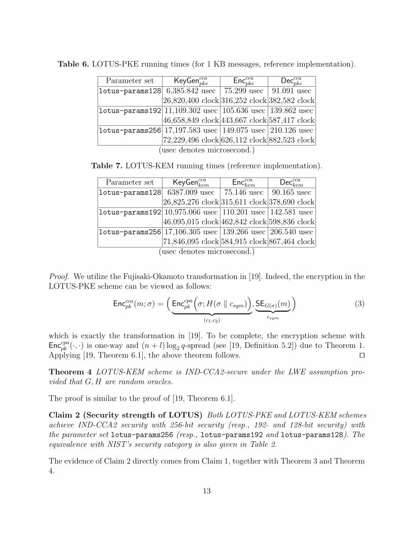
Table 6. LOTUS-PKE running times (for 1 KB messages, reference implementation).
Parameter set KeyGenccapke Encccapke Decccapkelotus-params128 6,385.842 usec 75.299 usec 91.091 usec
26,820,400 clock 316,252 clock 382,582 clocklotus-params192 11,109.302 usec 105.636 usec 139.862 usec
46,658,849 clock 443,667 clock 587,417 clocklotus-params256 17,197.583 usec 149.075 usec 210.126 usec
72,229,496 clock 626,112 clock 882,523 clock(usec denotes microsecond.)
Table 7. LOTUS-KEM running times (reference implementation).
Parameter set KeyGenccakem Encccakem Decccakemlotus-params128 6387.009 usec 75.146 usec 90.165 usec
26,825,276 clock 315,611 clock 378,690 clocklotus-params192 10,975.066 usec 110.201 usec 142.581 usec
46,095,015 clock 462,842 clock 598,836 clocklotus-params256 17,106.305 usec 139.266 usec 206.540 usec
71,846,095 clock 584,915 clock 867,464 clock(usec denotes microsecond.)
Proof. We utilize the Fujisaki-Okamoto transformation in [19]. Indeed, the encryption in theLOTUS-PKE scheme can be viewed as follows:
Encccapk (m;σ) =(Enccpapk
(σ;H(σ ‖ csym)
)︸ ︷︷ ︸
(c1,c2)
, SEG(σ)(m)︸ ︷︷ ︸csym
)(3)
which is exactly the transformation in [19]. To be complete, the encryption scheme withEnccpapk (·, ·) is one-way and (n + l) log2 q-spread (see [19, Definition 5.2]) due to Theorem 1.Applying [19, Theorem 6.1], the above theorem follows. ut
Theorem 4 LOTUS-KEM scheme is IND-CCA2-secure under the LWE assumption pro-vided that G,H are random oracles.
The proof is similar to the proof of [19, Theorem 6.1].
Claim 2 (Security strength of LOTUS) Both LOTUS-PKE and LOTUS-KEM schemesachieve IND-CCA2 security with 256-bit security (resp., 192- and 128-bit security) withthe parameter set lotus-params256 (resp., lotus-params192 and lotus-params128). Theequivalence with NIST’s security category is also given in Table 2.
The evidence of Claim 2 directly comes from Claim 1, together with Theorem 3 and Theorem4.
13
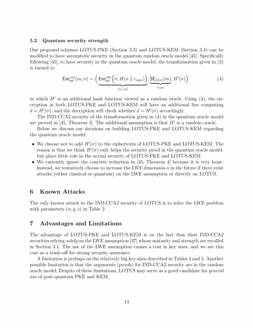
5.2 Quantum security strength
Our proposed schemes LOTUS-PKE (Section 3.3) and LOTUS-KEM (Section 3.4) can bemodified to have asymptotic security in the quantum random oracle model [45]. Specificallyfollowing [45], to have security in the quantum oracle model, the transformation given in (3)is turned to
Encccapk (m;σ) =(Enccpapk
(σ;H(σ ‖ csym)
)︸ ︷︷ ︸
(c1,c2)
, SEG(σ)(m)︸ ︷︷ ︸csym
, H ′(σ))
(4)
in which H ′ is an additional hash function viewed as a random oracle. Using (4), the en-cryption in both LOTUS-PKE and LOTUS-KEM will have an additional line computingd = H ′(σ), and the decryption will check whether d = H ′(σ) accordingly.
The IND-CCA2 security of the transformation given in (4) in the quantum oracle modelare proved in [45, Theorem 4]. The additional assumption is that H ′ is a random oracle.
Below we discuss our decisions on building LOTUS-PKE and LOTUS-KEM regardingthe quantum oracle model:
• We choose not to add H ′(σ) to the ciphertexts of LOTUS-PKE and LOTUS-KEM. Thereason is that we think H ′(σ) only helps the security proof in the quantum oracle model,but plays little role in the actual security of LOTUS-PKE and LOTUS-KEM.• We currently ignore the concrete reduction in [45, Theorem 4] because it is very loose.
Instead, we tentatively choose to increase the LWE dimension n in the future if there existattacks (either classical or quantum) on the LWE assumption or directly on LOTUS.
6 Known Attacks
The only known attack to the IND-CCA2 security of LOTUS is to solve the LWE problemwith parameters (n, q, s) in Table 2.
7 Advantages and Limitations
The advantage of LOTUS-PKE and LOTUS-KEM is on the fact that their IND-CCA2securities relying solely on the LWE assumption [37] whose maturity and strength are recalledin Section 3.1. The use of the LWE assumption causes a cost in key sizes, and we see thiscost as a trade-off for strong security assurance.
A limitation is perhaps on the relatively big key sizes described in Tables 4 and 5. Anotherpossible limitation is that the arguments (proofs) for IND-CCA2 security are in the randomoracle model. Despite of these limitations, LOTUS may serve as a good candidate for generaluse of post-quantum PKE and KEM.
14
References
1. Data Age 2025: The Evolution of Data to Life-Critical. http://www.seagate.com/files/www-content/
our-story/trends/files/Seagate-WP-DataAge2025-March-2017.pdf.
2. M. R. Albrecht. On dual lattice attacks against small-secret LWE and parameter choices in helib and SEAL.In Advances in Cryptology - EUROCRYPT 2017 - 36th Annual International Conference on the Theory andApplications of Cryptographic Techniques, Paris, France, April 30 - May 4, 2017, Proceedings, Part II, pages103–129, 2017.
3. M. R. Albrecht, C. Cid, J. Faugere, R. Fitzpatrick, and L. Perret. On the complexity of the BKW algorithm onLWE. Des. Codes Cryptography, 74(2):325–354, 2015.
4. M. R. Albrecht, R. Player, and S. Scott. On the concrete hardness of learning with errors. Cryptology ePrintArchive, Report 2015/046, 2015.
5. Y. Aono, X. Boyen, L. T. Phong, and L. Wang. Key-private proxy re-encryption under LWE. In G. Paul andS. Vaudenay, editors, INDOCRYPT, volume 8250 of Lecture Notes in Computer Science, pages 1–18. Springer,2013.
6. Y. Aono, T. Seito, and J. Shikata. A theoretical cost lower bound of lattice vector enumeration. ComputerSecurity Symposium 2017 (CSS2017), 1E4-5, 2017.
7. Y. Aono, Y. Wang, T. Hayashi, and T. Takagi. Improved progressive BKZ algorithms and their precise costestimation by sharp simulator. IACR Cryptology ePrint Archive, 2016:146, 2016.
8. B. Applebaum, D. Cash, C. Peikert, and A. Sahai. Fast cryptographic primitives and circular-secure encryptionbased on hard learning problems. In S. Halevi, editor, CRYPTO, volume 5677 of Lecture Notes in ComputerScience, pages 595–618. Springer, 2009.
9. S. Bai, T. Laarhoven, and D. Stehle. Tuple lattice sieving. LMS Journal of Computation and Mathematics,19(A):146–162, 2016.
10. W. Banaszczyk. New bounds in some transference theorems in the geometry of numbers. Mathematische Annalen,296(1):625–635, 1993.
11. W. Banaszczyk. Inequalities for convex bodies and polar reciprocal lattices in Rn. Discrete & ComputationalGeometry, 13(1):217–231, 1995.
12. Z. Brakerski, A. Langlois, C. Peikert, O. Regev, and D. Stehle. Classical hardness of learning with errors. InSymposium on Theory of Computing Conference, STOC’13, Palo Alto, CA, USA, June 1-4, 2013, pages 575–584,2013.
13. M. R. Bremner. Lattice Basis Reduction: An Introduction to the LLL Algorithm and Its Applications. CRCPress, Inc., Boca Raton, FL, USA, 1st edition, 2011.
14. Y. Chen and P. Q. Nguyen. BKZ 2.0: Better lattice security estimates. In D. H. Lee and X. Wang, editors,ASIACRYPT 2011, volume 7073 of Lecture Notes in Computer Science, pages 1–20. Springer, 2011.
15. I. Chillotti, N. Gama, M. Georgieva, and M. Izabachene. Faster fully homomorphic encryption: Bootstrappingin less than 0.1 seconds. In Advances in Cryptology - ASIACRYPT 2016 - 22nd International Conferenceon the Theory and Application of Cryptology and Information Security, Hanoi, Vietnam, December 4-8, 2016,Proceedings, Part I, pages 3–33, 2016.
16. R. Clercq, S. S. Roy, F. Vercauteren, and I. Verbauwhede. Efficient software implementation of Ring-LWEencryption. Cryptology ePrint Archive, Report 2014/725, 2014. http://eprint.iacr.org/2014/725.
17. T. F. development team. fplll, a lattice reduction library. Available at https://github.com/fplll/fplll, 2016.
18. U. Fincke and M. Pohst. Improved methods for calculating vectors of short length in a lattice, including acomplexity analysis. J-MATH-COMPUT, 44(170):463–471, Apr. 1985.
19. E. Fujisaki and T. Okamoto. Secure integration of asymmetric and symmetric encryption schemes. J. Cryptology,26(1):80–101, 2013.
20. M. Fukase and K. Kashiwabara. An accelerated algorithm for solving SVP based on statistical analysis. JIP,23(1):67–80, 2015.
21. N. Gama and P. Q. Nguyen. Predicting Lattice Reduction, pages 31–51. Springer Berlin Heidelberg, Berlin,Heidelberg, 2008.
22. N. Gama, P. Q. Nguyen, and O. Regev. Lattice enumeration using extreme pruning. In H. Gilbert, editor,EUROCRYPT 2010, volume 6110 of Lecture Notes in Computer Science, pages 257–278. Springer, 2010.
23. R. Kannan. Improved algorithms for integer programming and related lattice problems. In D. S. Johnson,R. Fagin, M. L. Fredman, D. Harel, R. M. Karp, N. A. Lynch, C. H. Papadimitriou, R. L. Rivest, W. L. Ruzzo,and J. I. Seiferas, editors, STOC, pages 193–206. ACM, 1983.
15
24. S. V. Khrushchev. Men′shov’s correction theorem and Gaussian processes (translated from Russian). Trudy Mat.Inst. Steklov., 155:151–181, 1981.
25. D. E. Knuth and A. C. Yao. The complexity of non-uniform random number generation. Algorithms andComplexity, Academic Press, New York, pages 357–428, 1976.
26. A. K. Lenstra, H. W. Lenstra, Jr., and L. Lovasz. Factoring polynomials with rational coefficients. MathematischeAnn., 261:513–534, 1982.
27. R. Lindner and C. Peikert. Better key sizes (and attacks) for LWE-based encryption. In A. Kiayias, editor,CT-RSA, volume 6558 of Lecture Notes in Computer Science, pages 319–339. Springer, 2011.
28. M. Liu and P. Q. Nguyen. Solving BDD by enumeration: An update. In E. Dawson, editor, CT-RSA, volume7779 of Lecture Notes in Computer Science, pages 293–309. Springer, 2013.
29. V. Lyubashevsky. Lattice signatures without trapdoors. Cryptology ePrint Archive, Report 2011/537, 2011.https://eprint.iacr.org/2011/537. Full version of a paper appearing at Eurocrypt 2012.
30. V. Lyubashevsky and D. Micciancio. On Bounded Distance Decoding, Unique Shortest Vectors, and the MinimumDistance Problem, pages 577–594. Springer Berlin Heidelberg, Berlin, Heidelberg, 2009.
31. D. Micciancio and O. Regev. Lattice-based cryptography. In Post-Quantum Cryptography, pages 147–191.Springer, 2009.
32. D. Micciancio and M. Walter. Practical, predictable lattice basis reduction. In Proceedings, Part I, of the35th Annual International Conference on Advances in Cryptology — EUROCRYPT 2016 - Volume 9665, pages820–849, New York, NY, USA, 2016. Springer-Verlag New York, Inc.
33. National Institute of Standards and Technology (NIST). Submission requirements and evaluation criteriafor the post-quantum cryptography standardization process. Website: http://csrc.nist.gov/groups/ST/
post-quantum-crypto/documents/call-for-proposals-final-dec-2016.pdf.34. P. Q. Nguyen and D. Stehle. LLL on the Average, pages 238–256. Springer Berlin Heidelberg, Berlin, Heidelberg,
2006.35. P. Q. Nguyen and B. Valle. The LLL Algorithm: Survey and Applications. Springer Publishing Company,
Incorporated, 1st edition, 2009.36. C. Peikert. Lattice cryptography for the internet. In M. Mosca, editor, Post-Quantum Cryptography - 6th
International Workshop, PQCrypto 2014. Proceedings, volume 8772 of Lecture Notes in Computer Science, pages197–219. Springer, 2014.
37. O. Regev. On lattices, learning with errors, random linear codes, and cryptography. In H. N. Gabow and R. Fagin,editors, STOC, pages 84–93. ACM, 2005.
38. O. Regev. The learning with errors problem (invited survey). In Proceedings of the 25th Annual IEEE Conferenceon Computational Complexity, CCC 2010, 2010, pages 191–204, 2010.
39. S. S. Roy, F. Vercauteren, and I. Verbauwhede. High precision discrete gaussian sampling on FPGAs. In SelectedAreas in Cryptography - SAC 2013 - 20th International Conference, 2013, pages 383–401, 2013.
40. M. Schneider and N. Gama. SVP challenge. Available at http://www.latticechallenge.org/svp-challenge/.41. C. Schnorr. A hierarchy of polynomial time lattice basis reduction algorithms. Theoretical Computer Science,
53(2):201 – 224, 1987.42. C.-P. Schnorr. Lattice reduction by random sampling and birthday methods. In H. Alt and M. Habib, editors,
STACS 2003, volume 2607 of Lecture Notes in Computer Science, pages 145–156. Springer, 2003.43. C. P. Schnorr and M. Euchner. Lattice basis reduction: Improved practical algorithms and solving subset sum
problems. In Math. Programming, pages 181–191, 1993.44. C.-P. Schnorr and H. H. Horner. Attacking the Chor-Rivest cryptosystem by improved lattice reduction. In L. C.
Guillou and J.-J. Quisquater, editors, EUROCRYPT 1995, volume 921 of Lecture Notes in Computer Science,pages 1–12. Springer, 1995.
45. E. E. Targhi and D. Unruh. Quantum security of the Fujisaki-Okamoto and OAEP transforms. CryptologyePrint Archive, Report 2015/1210, 2015. http://eprint.iacr.org/2015/1210.
46. S. S. Venkatesh. The theory of probability: Explorations and applications. Cambridge: Cambridge UniversityPress, 2013.
16
Appendix
A Hardness Estimation and Proposed Parameters for LWE inLOTUS
Our parameter sets lotus-params128, lotus-params192, and lotus-params256 are basedon the theory to bound the cost of lattice based attack for LWE presented recently by Aonoet al. in [6]. This section is mainly based on [6], with additional contents dedicated to theLWE assumption.
The lattice based attacks against an LWE instance with parameter (n, q, s) consisting ofthree steps:
(i) construct a lattice basis B from the instance,(ii) perform lattice reduction for B, and(iii) solve the bounded distance decoding corresponding to LWE.
This attack model is completely the same as Liu-Nguyen [28], and typically called “theprimal attack.” The attacker’s cost is given as follows and the minimum is over all latticereduction algorithms and the success probability of the point search algorithm.
Cost(Problem) = minCost(LatticeReduction) + Cost(PointSearch)
Success probability of PointSearch. (5)
Roughly speaking, if one uses a stronger algorithm, the cost of lattice reduction increases,as that of point search is decreases.
A.1 Technical backgrounds
A.1.1 Basic notations and special functions
Let Z and Zm are the set of integers and the ring {0, . . . ,m − 1} respectively. Q and Rare the set of rational numbers and real numbers respectively. For natural numbers n ≤ m,[n,m] is the set {n, . . . ,m} ⊂ Z and we denote [m] := [1,m]. Throughout this paper, m andk are usually used for the considered and projected dimension respectively.
The gamma and beta functions are respectively defined by
Γ (a) =
∫ ∞0
ta−1e−tdt and B(a, b) =
∫ 1
0
za−1(1− z)b−1dz.
The basic relations Γ (a+ 1) = aΓ (a) and B(a, b) = Γ (a)Γ (b)/Γ (a+ b) hold.For m ∈ N, let Bm(x, c) be the m-dimensional ball whose center is x ∈ Rm and radius
c > 0. The center-origin ball is denoted by Bm(c) := Bm(0, c). The volume of m-dimensional
ball with radius c is Vm(c) = πm/2cm
Γ (m2+1)
. In particular, we denote Vm := Vm(1). Also, Sm(r) is
the surface of Bm(r). The log function log(·) is always the natural logarithm.
17

Incomplete gamma function: For a parameter a, the lower incomplete gamma functionregularized lower incomplete gamma function are
γ(a, x) :=
∫ x
0
ta−1e−tdt and P (a, x) =γ(a, x)
Γ (a)
respectively. P (a, x) can be used for the closed formula of the high-dimensional Gaussianintegral.∫
Bk(ρ)
1
ske−π‖x‖
2/s2dx =2πk/2
skΓ (k2)
∫ ρ
0
e−πr2/s2rk−1dr =
1
Γ (k2)γ
(k
2,πρ2
s2
)= P
(k
2,πρ2
s2
).
(6)
By the relation P (a, x) ≤ 1
Γ (a)
∫ x
0
ta−1dt =xa
aΓ (a), we can bound the inverse function
of P from lower:P−1(a, x) ≥ (aΓ (a)x)1/a. (7)
Beta distribution and incomplete beta function: For a, b > 0, the beta distributionB(a, b) is defined by the probability density function
f(x; a, b) =xa−1(1− x)b−1
B(a, b).
Its cumulative distribution function is given by the incomplete beta function:
Ix(a, b) :=1
B(a, b)
∫ x
0
za−1(1− z)b−1dz,
and its inverse function is defined by x = I−1y (a, b)⇔ y = Ix(a, b). Both functions are strictlyincreasing from [0, 1] to [0, 1].
A bound
Ix(a, b) ≤1
B(a, b)
∫ x
0
za−1dz =xa
a ·B(a, b)
holds and thusI−1x (a, b) ≥ (aB(a, b)x)1/a. (8)
Fact 1 Suppose (x1, . . . , xm) ← Sm(1). Then, x21 + · · · + x2k follows the beta distribution ofparameters (a, b) =
(k2, m−k
2
). Thus,
Pr(x1,...,xm)←Sm(1)
[x21 + · · ·+ x2k ≤ C
]= IC
(k
2,m− k
2
):=
∫ C0x
k2−1(1− x)
m−k2−1dx
B(k2, m−k
2)
.
In particular, (x1, . . . , xm−2) follows the uniform distribution in Bm−2(1), which impliesthe following formula.
Pr(x1,...,xm)←Bm(1)
[x21 + · · ·+ x2k ≤ C
]= IC
(k
2,m+ 2− k
2
).
18
A.1.2 Basics on lattices
This section is an outline of lattices which are used to construct our theory. For morefundamental explanations and backgrounds, readers should refer the textbooks [13,35].
For a set of linearly independent vectors b1, . . . , bn ∈ Qm, the lattice is defined by the setof all the integer linear combination:
L(b1, . . . , bn) =
{n∑i=1
aibi : ai ∈ Z
}.
The ordered set (b1, . . . , bn) is called a basis of lattice. For a basis, its Gram-Schmidtbasis is defined by recursively b∗1 = b1 and b∗i = bi−
∑i−1j=1 µi,jb
∗j where µi,j = 〈bi, b∗j〉/〈b∗j , b∗j〉
for i = 2, . . . , n. The new basis b∗1, . . . , b∗n that are orthogonal to each other spans the same
space to the original basis:
span(L) :=
{n∑i=1
wibi : wi ∈ R
}=
{n∑i=1
xib∗i : xi ∈ R
}.
Thus, any lattice point v =∑n
i=1 aibi can be represented by using Gram-Schmidt basis:v =
∑ni=1 xib
∗i . For this, the j-th projection is
πj(v) =n∑i=j
xib∗i .
The volume of lattice vol(L) is defined by
| det(L)| =n∏i=1
‖b∗i ‖.
Hard lattice problems: For a lattice L, we denote by λ1(L) the smallest nonzero norm ofpoints in L, i.e., the length of the shortest vector. The problem for searching v ∈ L such that‖v‖ = λ1(L) is called the shortest vector problem (SVP). The approximate Hermite shortestvector problem (HSVPα) [21] is the problem of finding vector v shorter than α · vol(L)1/n.The bounded distance decoding (BDD) problem 3 for a given lattice basis B, target point tand the distance d, is the problem of finding a lattice point v such that ‖v − t‖ ≤ d.
Gaussian heuristic [44, Section. 3]: Consider a set S ⊂ span(L) with a finite volume:vol(S) < ∞. The Gaussian heuristic assumption claims that the number of lattice pointsin S is approximately given by vol(S)/vol(L). In particular, we can see λ1(L) is close to
` = V−1/nn vol(L)1/n so that Vn(`) = vol(L). We denote this length by GH(L) and call it the
Gaussian heuristic length of L.
3 The standard version of BDD is defined by using the shortest vector length λ1(B); see, for example Lyubashevskyand Micciancio [30]. Throughout this paper, we use this notation by following the work of Liu and Nguyen [28].
19

Dual lattices: For a lattice L, its dual lattice L× is defined by the set
L× = {w ∈ span(L) : ∀v ∈ L, 〈v,w〉 ∈ Z}.
For the basis matrix B = (b1, . . . , bn) ∈ Rm×n, its dual basis matrix D = (d1, . . . ,dn)satisfies BTD = I. Explicitly written, D = B(BTB)−1 in general and D = (BT )−1 for thesquare matrix B.
Fact 2 Let (dn, . . . ,d1) be the reversed order of dual basis of (b1, . . . , bn). Its Gram-Schmidtorthogonalization (d?n, . . . ,d
?1) satisfies d?i = b∗i /‖b∗i ‖2.
Thus, ‖d?i ‖ = 1/‖b∗i ‖ holds and it deduces vol(L×) = 1/vol(L). The Gaussian heuristicover the dual lattice predicts that
λ1(L×) ≈ V −1/nn vol(L×)1/n = V −1/nn vol(L)−1/n.
Lattice basis reduction: Since the celebrated LLL algorithm [26], a series of lattice reduc-tion algorithm has wide applications in many area. In general, such an algorithm selects asuitable unimodular matrix U for given lattice basis matrix B, update the basis by multipli-cation: B ← B ·U . In this document, we focus on these algorithms as the approximate SVPalgorithm as [14,41,43,44]. The strongest lattice reduction algorithm finds the shortest vec-tor at the first vector b1 of basis. The Gaussian heuristic suggests the practical lower (resp.upper) bounds of ‖b1‖ (resp. ‖b∗n‖), that is, for a majority of random lattices, its reducedbasis satisfies
‖b1‖ > GH(L) = V −1/nn · vol(L)1/n and ‖b∗n‖ < GH(L×) = V 1/nn · vol(L)1/n.
We also claim the following assumption to prove Lemma 1 in Section A.3.2, which is abit stronger than the original Gaussian heuristic.
Assumption 1 For almost all lattices and its reduced basis (b1, . . . , bm), its projections allsatisfy
‖b∗n‖ < GH(L×) = V 1/nn · (‖b1‖ · · · ‖b∗n‖)1/n
for a reasonable range of n, such as (3/4)m ≤ n ≤ m.
Root-Hermite factor and geometric series assumption: From the experimental ob-servations by Gama, Nguyen and Stehle [21, 34] for lattice reduction algorithms that workon any lattice dimension n, there exists a constant δ0 so that the output of lattice reductionalgorithm over random lattices satisfies ‖b1‖ ≈ δn0 vol(L)1/n. This δ0 is called the root Hermitefactor of the algorithm. We call the basis is δ0-reduced if ‖b1‖ ≤ δn0 vol(L)1/n holds, thus, itis a solution of the HSVPδn0
problem.Depending on varieties of algorithms, the graph of Gram-Schmidt lengths ‖b∗i ‖ has a
variety if they all achieve the same root Hermite factor δ0. However, they are typicallyconcave curves close to a line. Schnorr’s geometric series assumption (GSA) [42] claims that
20

||b∗i ||2 is approximated by ||b1||2ri−1 by a constant r < 1. Hence, each of Gram-Schmidtlengths of a δ0-reduced basis can be approximated by
||b∗i || = r2i−1−n
4 vol(L)1/n where r = δ−4nn−1
0 . (9)
We call the sequence
(||b∗1||, . . . , ||b∗n||) = (r(1−n)/4vol(L)1/n, . . . , r(n−1)/4vol(L)1/n)
the δ0-GSA basis, and sometimes we denote it by Bδ0 , which is an abused notation becauseit is not a lattice basis.
This assumption has been used to estimate the practical complexity of lattice problems insome published works [20,27]. However, for highly reduced lattice bases, the lengths ‖b∗i ‖ donot follow a line in the last indexes. Such phenomenon is justified by the Gaussian heuristic.Hence, it is not reasonable to estimate the expected complexity by using GSA. On the otherhand, we will demonstrate it can be used to estimate a lower bound in Section A.3.
A.1.3 Lattice-based attack against LWE
Definition 1. (Search learning with errors (LWE) problem with Gaussian error) Fixing theproblem parameter n,m, q ∈ N and α ∈ R, the challenger generates random vectors ai ∈ Znq(i = 1, . . . ,m), a secret vector s ∈ Znq , and a random Gaussian noise vector e ∈ Zm whosecoordinates are independently and randomly sampled from the discrete Gaussian distributionDs whose probability density function at i ∈ Z is
p(i) =e−πi
2/s2∑∞j=−∞ e
−πj2/s2 . (10)
Then, the adversary gets pairs (ai, bi = 〈ai, s〉 + ei mod q) ∈ Znq × Zq for i = 1, . . . ,mand tries to recover the secret vector s.
For the uniqueness of the solution, the number of vectors m is usually taken much largerthan n. The primal attack for LWE which we will consider in the later section is convertingthe instance to a BDD instance with a lattice of rank m′ ≤ m which is selected by theattacker to minimize the cost.
We introduce an outline of the primal attack. From the instance, suppose we pick somevectors and construct a matrix A ∈ Zn×m′q by concatenating a1, . . . ,am′ . Then, As + e =
b (mod q) holds and there exists an integer vector w ∈ Zm′q , the equation can be expressedby As + qw + e = b. Thus, the unknown vectors s and w satisfy
[A qI]
[sw
]+ e = b
and if the error vector is short, there exists a point of lattice spanned by the columns of[A qI] ∈ Zm′×(m′+n) close to b. Since the basis given by the matrix is degenerate, it needs
21

to reconstruct the independent vectors for which we know an efficient method. Therefore,the LWE problem is regarded as a variant of BDD problem whose distance is ‖e‖. Since thedistribution of ‖e‖ is well-known, we can take an appropriate bound so that the error vectoris shorter than it with high probability.
A.1.4 Enumeration algorithm and cost estimation
We give a brief overview of the lattice vector enumeration algorithms by Kannan [23],and Fincke-Phost [18], pruned enumeration by Schnorr [44], and rigid analysis under theGaussian heuristic assumption by Gama-Nguyen-Regev [22].
For a given lattice basis (b1, . . . , bm), suppose we have data of Gram-Schmidt vectorsb∗i and Gram-Schmidt coefficients µi,j with sufficient accuracy. The enumeration algorithmfinds combination of coefficients ai such that v =
∑ni=1 aibi ∈ L is shorter than a threshold
radius c. It is easy to convert the coefficients to the lattice vector.The standard pruned enumeration algorithm takes as input the Gram-Schmidt vectors
and coefficients, thresholding radius c, and pruning coefficients 0 < R1 ≤ . . . ≤ Rm = 1. Itsearches the (possibly infinite) labelled tree of depth m. Each node at depth k is labelledby a vector v ∈ Rm and the projective length ‖πm−k+1(v)‖, and it has children labelled byvectors v + am−kbm−k (am−k ∈ Z). The root has the zero vector. Hence, every node at depthk has the label
∑mi=m−k+1 aibi. The algorithm carries out the depth-first search and pruning
the edge when the projective length exceeds c · Rk at depth k to limit the searching space.For the detailed algorithm and efficient implementation, see for example [22,43].
We remark that it can be easily extended to the algorithm for the BDD problem [28];the projective length corresponding to the label v is changed to ‖πm−k+1(v − t)‖ where t isthe target vector.
These enumeration algorithms output all lattice vectors satisfying ‖v‖ ≤ c (or ‖v−t‖ ≤ c)if there is no pruning, i.e., Ri = 1 for all i.
Cost estimation under the model by Gama-Nguyen-Regev [22]: They gave modelsand efficient techniques for analyzing success probability and complexity for the prunedenumeration. For given searching radius c and pruning coefficients, The space searched bythe above tree-searching algorithm at depth k is
{v ∈ Rk : ‖πk−i+1(v)‖ ≤ c ·Ri for i ∈ [k]}
=
{m∑
j=m−k+1
xjb∗i :
m∑j=m−i+1
x2j‖b∗j‖2 ≤ (c ·Ri)2 for i ∈ [k]
}.
(11)
Thus, by using the appropriate rotation that transforms the point∑m
j=m−k+1 xjb∗i into
(xm−k+1‖b∗m−k+1‖, . . . , xm‖b∗m‖), we can find that the searching space is the rotation of theobject {
(x1, . . . , xk) ∈ Rk :∑i=1
x2i < (c ·R`)2 for ∀` ∈ [k]
}.
22

For simplicity, one can define the set Ck as below
Ck =
{(x1, . . . , xk) ∈ Rk :
∑i=1
x2i < R2` for ∀` ∈ [k]
}. (12)
By the Gaussian heuristic over the projective sublattice πm−k(B), the number of latticepoints in the space (11) is
ckvol(Ck)∏mi=m−k+1 ‖b∗i ‖
,
and is the approximation of the number of touched nodes at depth k. Therefore, the cost ofenumeration, which is defined by the total number of nodes touched by the tree searchingalgorithm, is given as follows.
N =1
2
m∑k=1
ckvol(Ck)∏mi=m−k+1 ‖b∗i ‖
. (13)
Note that the factor 1/2 comes from the symmetry in the shortest vector computation, andit is vanished when we consider the closest vector problem and its variants.
A.1.5 Complexity measurements
Several measurements have been proposed for security estimation whereas our estimationis based on the number of nodes searched in the enumeration tree [22,28]. However, we needto be careful to compare other measurements such as computing time in seconds [4, 27] orthe number of logical gates.
A typical efficient implementation of tree searching algorithm needs to compute theinteger linear combination of Gram-Schmidt coefficients
m∑i=m−k+1
yiµi,m−k+1 (14)
by floating numbers with some accuracy to check whether the square of projective length‖πm−k+1(v)‖2 = s2 + (computed term in above k − 1 terms ) exceeds the bound. That is,the complexity to check a node at depth k includes k+ 1 multiplication, (k− 1) + 1 additionand 1 comparison operations over floating numbers. Denoting the cost depending on eachmeasurement for a node at depth k by CostMeasure(k), the complexity is evaluated as
ECModel,single,Measure(B; params) =1
2
m∑k=1
ckvol(Ck) · CostMeasure(k)∏mi=m−k+1 ‖b∗i ‖
. (15)
Here, B and parmas are respectively the lattice basis and given parameters for models suchas success probability.
23

Since our target is the lower bounds, we provide how many costs are required at minimumin each unit to process one node in the searching tree. In other words, we propose how tobound CostMeasure(k) from lower for Measure ∈ {gates, time}, which means that in themeasure of number of logical gates as required in the NIST’s criteria [33], and in the single-thread CPU time.
Below we assume that floating point numbers with a suitable precision are used to ap-proximate and compute the Gram-Schmidt coefficients and lengths.
Computing time in seconds: To the best of our knowledge, the currently known fastestimplementation for lattice vector enumeration can process about 5.0 · 107 nodes per secondin a single thread in a practical dimension about 100. (A bit less than 6.0 · 107 in [7] andabout 3.3 · 107 in [32]).
On the other hand, since the latest CPU can carry out many floating point operationsper a cycle, a highly optimized implementation for each CPU can be faster. For example, thelatest Intel CPU has two fused multiply add (FMA) units that can compute in one clock thevector multiplication operation (a1, . . . , a8) · (b1, . . . , b8) 7→ (a1 · b1, . . . , a8 · b8) and vector sumoperation (a1, . . . , a8) 7→
∑8i=1 ai over eight 64-bit floating point numbers. Thus, the sum
(14) at depth k can be computed in 2dk/8e cycle clocks in theory that neglects the speed ofmemory transfer. Assuming the computation of squaring and comparison can be done in 2cycle clocks, the total clock cycles need to process the node at depth k is at least 2dk/8e+ 2.Furthermore, since recent common CPUs can work in about 5GHz clock at maximum in astandard environment, the timing cost lower bound would be
Costtime(k) = 2.0 · 10−10 · (dk/8e+ 2) (16)
This is about 10 times faster than the known fastest implementation for dimensions satisfying(dk/8e+ 2) = 10.
Hence, substituting it to (15), we get
ECModel,single,time(B; params) > 10−10 ·m∑k=1
ckvol(Ck) · (dk/8e+ 2)∏mi=m−k+1 ‖b∗i ‖
[sec]. (17)
and will give our theoretical lower bound by providing inequality for vol(Ck).
Number of logical gates: By the argument in Section A.3.2, we can claim the minimumdimension n used in the lattice reduction, which is slightly smaller than the whole latticedimension m in enumeration. The experimental heuristic analysis by Nguyen-Stehle [34,Heuristic. 4] claims that d = 0.25n+ o(n) bits are necessary for the mantissa in the floatingpoint operation 4 to carry out the LLL algorithm. Since it has a small order term, consideringa margin, we assume that d = b0.2nc bits is the lower bound of necessary precision.
We estimate the number of necessary logical gates to treat this precision of floating pointnumbers by the following rule. To carry out the addition (resp. the multiplication) of floating
4 This is not the same as the bit-size of floating point numbers. For example, the standard 64-bit floating pointnumber has 53-bit length mantissa.
24
point numbers with d-bit mantissa, the necessary size of circuit can be bounded by the d-bitadder (resp. multiplier) respectively. A simple d-bit adder consists of d full-adders and eachone has typically 5 logical gates. Also, a simple d-bit times d′-bit multiplier also consists ofd · d′ full adders. Since the coefficients yi in the sum (14) are typically small integers, weassume they can be represented by 8 bits. Hence, a possible logical gate to compute summingcomputation (14) includes k multiplication of d-bit numbers and d′ = 8 bit integers, andk − 1 addition of d-bit numbers. Totally, it requires
Costgates(k) := k · d · 8 · 5 + (k − 1) · d · 5 = 45kd− 5d = 9kn− n (18)
logical gates at least. Again, substituting its local cost to (15), we obtain
ECModel,single,gates(B; params) >1
2
m∑k=1
ckvol(Ck) · (9km−m)∏mi=m−k+1 ‖b∗i ‖
. (19)
and the theoretical lower bound will be provided via our lower bound for vol(Ck).
A.1.6 Our complexity models
We define several models to discuss the complexity of enumeration algorithm. Fromnow on, we use ECModel,Alg,Measure(B; params) to denote the optimal enumeration cost(15) where the target model Model ∈ {prob,many, LWE}, usage of enumeration algo-rithm Alg ∈ {single,multi}, and complexity measurement Measure ∈ {nodes, gates, time},which will be defined in this section. Moreover, we will use UBModel,Alg,Measure(B; params)and LBModel,Alg,Measure(B; params) for the upper bounds (in Section A.5.1) and the lowerbounds (in Section A.2), respectively.
Particularly, we will use LBmany,multi,Measure(B;N = 1, c) for the lower bound of latticereduction algorithm and use LBLWE,multi,Measure(B; p, s) for the lower bound of attackingLWE problem and our parameter setting.
In the approximation setting such as the approximate SVP, there exist many target points.By the Gaussian heuristic, the number of lattice points shorter than c within the searchingarea c ·Ck is about N = cmvol(Cm)/vol(L). Thus, the best enumeration algorithm expectedto find N lattice points is given by best combination of (R1, . . . , Rm) that minimizes (15)subject to that vol(Cm) ≥ Nvol(L)/cm. We denote this cost by ECmany,single,Measure(B;N, c).where single denotes the single usage of enumeration subroutine, B is the input latticebasis, and Measure ∈ {nodes, gates, time} means that we use CostMeasure(k) to measurethe complexity.
The multiple usage of enumeration subroutine is considered by Gama-Nguyen-Regev [22].For a given number N of wanted target points, one can run M trials of enumeration with asmall target number N/M which might not be an integer. The total cost is the sum of (M−1)randomizations, (M − 1) lattice reductions, and M enumerations with the low probability.We denote such cost by
ECmany,multi,Measure(B;N, c):= minM [(M − 1) · Cost(LatticeReduction) +M · ECmany,single,Measure(B;N/M, c)].
25

Hence, we finished the definition of ECmany,Alg,Measure(B;N, c).Another interesting situation is the unique setting. It is a special situation of BDD prob-
lem with instance (B, t) where the distribution D of error vector e = t− v is known. In thesituation where we want to recover the error, searching radius is not fixed since the rangeof error distribution is not limited in general. Suppose we have an optimized radius andbounding coefficients which derive the searching space
Um =
{(x1, . . . , xm) :
∑i=1
x2i < T 2i = (cRi)
2 for ∀ ` ∈ [m]
}.
Then, the success probability of the enumeration is given by the integral of fD(x) over thesearching space:
Prx←D
[x ∈ Um] =
∫Um
fD(x)dx. (20)
To analyse the LWE problem, we assume the error distribution is given by the continu-ous Gaussian whose probability density function is fLWE(x) = exp(−π‖x‖2/s2)/sm while atypical definition uses the discrete Gaussian. Such assumption makes us the discussion muchanalytic since the continuous density function is rotation invariant and matches the require-ment of our geometric lemma used for analysis. In other words, with using the radial basisfunction φe(r) = e−πr
2/s2/sm, we can write fLWE(x) = φe(‖x‖), and discuss a lower boundof cost (13) subject to that the success probability (20) is larger than the given threshold.
As the approximation setting, we use the notations ECLWE,single,Measure(B; p, s) andECLWE,multi,Measure(B; p, s) to denote the costs about the LWE problem.
Finally, we introduce the probability model by Gama-Nguyen-Regev [22]. Under thereasonable assumption ( [22, Assumption 3]), they assumed that the probability to find avector v with using searching radius c = ‖v‖ is given by
Pr(x1,...,xm)←Sm(‖v‖)
[∑i=1
x2i < ‖v‖2 ·R2` for ∀ ` ∈ [m]
]. (21)
Hence, the best enumeration algorithm of success probability p0 is given by best combi-nation of (R1, . . . , Rm) that minimizes (13) subject to that (25) is larger than p0. We denotesuch optimized cost by ECprob,single,Measure(B; p0, c). Also, as the approximation setting, thecost under the multiple usage of enumeration algorithm is
ECprob,multi,Measure(B; p, c):= minM [(M − 1) · Cost(LatticeReduction) +M · ECprob,single(B; p/M, c)].
A.2 Bounding cost for pruned lattice vector enumeration
A.2.1 Single usage of the enumeration algorithm
In order to bound the cost (15, we need to bound each volume factor vol(Ck) in (13).The following geometric lemma has a crucial role.
26
Lemma 4 Let Ck be a finite k-dimensional object, i.e., the k-dimensional volume vol(Ck) <∞. Let τk be the radius such that Vk(τk) = vol(Ck). Fix a radial basis function r(x) = φ(‖x‖)where φ(‖x‖) is a positive decreasing function on the radius: φ(x) ≥ φ(y) ≥ 0 for any0 ≤ x ≤ y. Then we have ∫
Ck
r(x)dx ≤∫Bk(τk)
r(x)dx. (22)
Noting that similar results where φ(x) is a Gaussian function is already known [24, Lemma7.1] and [46, Sect. 14.8] in another contexts and they also proved their claim by similarstrategies. For future discussions, we give the proof for generic φ(x).
Proof. By Vk(τk) = vol(Ck), it holds that V := vol(Ck \ Bk(τk)) = vol(Bk(τk) \ Ck). Sinceφ(‖x‖) is decreasing function, we have the inequalities∫
Ck\Bk(τk)
r(x)dx ≤ V · φ(τk) ≤∫Bk(τk)\Ck
r(x)dx.
Hence, ∫Ck
=
∫Ck∩Bk(τk)
+
∫Ck\Bk(τk)
≤∫Ck∩Bk(τk)
+
∫Bk(τk)\Ck
=
∫Bk(τk)
.
ending the proof. utBy using this lemma, we provide the lower bound complexity of the single and multiple
usages of Gama et al.’s pruned enumeration [22] for the approximation setting and unique(LWE) settings.
Approximation setting: Fixing the pruning coefficientsR1, . . . , Rm, the intermediate search-ing areas Ck are fixed by (12). Suppose we have an optimal set of pruning coefficients. Then,for any k ≤ m− 2,
N · vol(L)
cm≤ vol(Cm) =
∫Ck
vol{z ∈ Cm : (z1, . . . , zk) = x)}dx
≤∫Ck
vol{z ∈ Bm(1) : (z1, . . . , zk) = x)}dx
where the volumes are the (m−k)-dimensional ones defined on the coordinates (zk+1, . . . , zm).The latter integrating function
r(x) = vol{z ∈ Bm(1) : (z1, . . . , zk) = x)} =
{Bm−k(
√1− ‖x‖2) if ‖x‖ ≤ 1
0 if otherwise
satisfies the requirement of Lemma 4. Thus, we have
vol(Cm) ≤∫Bk(τk)
r(x)dx = Vm(1) · Iτ2k
(k
2,m+ 2− k
2
).
27

By the condition N ·vol(L)cm
≤ vol(Cm), we have the lower bound of the radius
τk ≥
√I−1N ·vol(L)/Vm(c)
(k
2,m+ 2− k
2
).
Substituting this bound with the equation Vk(τk) = vol(Ck) in Lemma 4 to (13), weobtain our lower bound for the enumeration to find N vectors shorter than c is given asfollows:
LBmany,single,Measure(B;N, c) =1
2
m∑k=1
ckVk(1)
[I−1Nvol(L)
Vn(c)
(k2, m+2−k
2
)]k/2· CostMeasure(k)∏n
i=n−k+1 ‖b∗i ‖.
(23)This is valid for the parameters satisfying Nvol(L) ≤ Vm(c).
Learning with errors setting: Since each Ck is the k-dimensional projection of Cm, wehave the inequality on the success probability. When the distribution is continuous GaussianCs, we have the relation
(20) = Prx←Cms
[x ∈ Cm] < Prx←Cms
[(x1, . . . , xk) ∈ Ck] = Prx←Cks
[(x1, . . . , xk) ∈ Ck] .
The RHS is∫Ckφe(‖x‖)dx where φe(‖x‖) = exp(−π‖x‖2/s2)/sk and the integral func-
tion meets the requirement of Lemma 4. Thus, combining with (6), we have the inequality
p <
∫Ck
φe(‖x‖)dx = P
(k
2,πτ 2ks2
)which implies the lower bound of the radius
τk ≥s√π
√P−1
(k
2, p
).
Hence, substituting this into (13) we obtain our lower bound as
LBLWE,single,Measure(B; p, s) =1
2
m∑k=1
(s/√π)kVk(1)
[P−1
(k2, p)] k
2 · CostMeasure(k)∏mi=m−k+1 ‖b∗i ‖
. (24)
Probability setting: In [22], they assume the probability model for the shortest vectorproblem. We introduce this model to use in the computer experiments to justify our newassumption (Assumption 2) although this model is not used for the LWE parameter setting.Under the reasonable assumption ( [22, Assumption 3]), the probability to find a vector vwith using searching radius c = ‖v‖ is given by
Pr(x1,...,xm)←Sm(‖v‖)
[∑i=1
x2i < ‖v‖2 ·R2` for ∀ ` ∈ [m]
]. (25)
28

Then, the probability (25) is bounded upper as
(25)≤ Prx←Sm(‖v‖)
[∑i=1
x2i < ‖v‖2 ·R2` for ∀ ` ∈ [m− 2]
](by relaxed condition)
= Prx←Bm−2(1)
[∑i=1
x2i < R2` for ∀ ` ∈ [m− 2]
]=
vol(Cm−2)
Vm−2(1).
(26)
This probability have a relation to the volume of cylinder intersection by
τk ≥
√I−1vol(Cm−2)/Vm−2(1)
(k
2,m− k
2
)≥
√I−1p
(k
2,m− k
2
).
Thus, as the same argument to the situation of approximation setting, we obtain ourlower bound for the enumeration of probability p and radius c:
LBprob,single,Measure(B; p, c) =1
2
m∑k=1
ckVk(1)[I−1p
(k2, m−k
2
)] k2 · CostMeasure(k)∏m
i=m−k+1 ‖b∗i ‖. (27)
A.2.2 Multiple usage of the enumeration algorithm
Using our lower bound for single usage of enumeration algorithm, we can bound the costof Gama-Nguyen-Regev’s extreme pruning that uses multiple random bases. As mentionedin Section A.1.4, the cost of multiple usage is given by
ECModel,multi,Measure(B; p) =minM [(M − 1) · Cost(LatticeReduction) +M · ECModel,single,Measure(B; p/M)]
where p stands for the success probability or the number of found vectors depending on themodel. We estimate the lower bound cost by neglecting the cost for the lattice reduction
ECModel,multi,Measure(B; p) > minM
[M · LBModel,single,Measure(B; p/M)] (28)
Remark that as we will show in the next section, the lower bound cost of lattice reduction isnot zero if we start with a random (LLL-reduced) basis. However, in the situation of extremepruning, the complete randomization, for instance, multiplying random unimodular matrixto the whole basis can achieve it, is too strong for our goal. Thus, in the sense of algorithmoptimization, the quality of basis after randomization may not far from the original reducedbasis if we have a good procedure as [2, Appendix. A] and [17]. This is the reason that weneglect the lattice reduction cost here. As we see in below, we do not need to consider thenumber M of used bases in the lower bounds.
In (29), (30) and (31) below, we use the notation C(k) for CostMeasure(k) for simplicity.
29

Approximation setting: For the target number N of lattice points that we want to findif we use M randomized bases, at least N/M target numbers are necessary for each basis. Itshould be larger than N/M because of duplication of the found vectors. For these parameters,by a similar argument as above, the cost is bounded lower by using (23), and by the inequality(8), we have
M · LBmany,single,Measure(B;N/M, c) >M
2
m∑k=1
ckVk(1)
[I−1Nvol(L)
MVm(c)
(k2, m+2−k
2
)]k/2· C(k)∏m
i=m−k+1 ‖b∗i ‖
>Nvol(L)
4Vm(c)
m∑k=1
Vk(c) · k ·B(k2, m+2−k
2
)· C(k)∏m
i=m−k+1 ‖b∗i ‖
=N
4
m∑k=1
[m−k∏i=1
‖b∗i ‖c
]· k · Vk(1)
Vm(1)·B(k
2,m+ 2− k
2
)· C(k)
=N
2
m∑k=1
[m−k∏i=1
‖b∗i ‖c√π
]· Γ(m+ 2− k
2
)· C(k) =
N
2
m∑k=1
[k∏i=1
‖b∗i ‖c√π
]· Γ(k + 2
2
)· C(m− k)
:= LBmany,multi,Measure(B;N, c).(29)
Remark that if N is fixed, increasing of c implies the decreasing cost and increasing thelength of found vectors.
Learning with Errors setting: We can show the cost lower bound of the primal attackby Liu-Nguyen [28] as follows:
M · LBLWE,single,Measure(B; p/M, s) >M
2
m∑k=1
(s/√π)kVk(1)
[P−1
(k2, pM
)] k2 · C(k)∏m
i=m−k+1 ‖b∗i ‖
>p
4
n∑k=1
(s/√π)kVk(1) · k · Γ (k/2) · C(k)∏n
i=n−k+1 ‖b∗i ‖=p
2
n∑k=1
sk · C(k)∏ni=n−k+1 ‖b∗i ‖
:= LBLWE,multi,Measure(B; p, s).
(30)
30
Probability setting: For the lower bound for Gama-Nguyen-Regev’s probabilistic model,we can show the lower bound by using (27) and (8):
M · LBprob,single,Measure(B; p/M, c) >M
2
m∑k=1
Vk(c)[I−1p/M
(k2, m−k
2
)] k2 · C(k)∏m
i=m−k+1 ‖b∗i ‖
>p
4
m∑k=1
Vk(c) · k ·B(k2, m−k
2
)· C(k)∏m
i=m−k+1 ‖b∗i ‖=p
2
m∑k=1
ckπk/2Γ (m−k2
) · C(k)
Γ (m2
)∏m
i=m−k+1 ‖b∗i ‖
=p
2Γ (m2
)vol(L)
m∑k=1
k∏i=1
‖b∗i ‖ · cm−kπm−k
2 Γ
(k
2
)· C(m− k)
=p · cmπm/2
2Γ (m2
)vol(L)
m∑k=1
[k∏i=1
‖b∗i ‖c√π
]· Γ(k
2
)· C(m− k) := LBprob,multi,Measure(B; p, c)
(31)
where the equality from the second line to the third line holds by swapping index m− k byk.
Concluding these inequalities, we have two remarks. First, we do not need to consider thenumber of randomized bases in the calculation of lower bounds. Second, since they are linearfunctions of probability or the number of target points, the speeding up of extreme pruningstrategy is bounded by a constant independent from the number of bases and probabilities.
A.3 Bounding cost of lattice problems
We introduce our formula to bound the cost of lattice reduction that achieves the rootHermite factor δ0. Unlike the argument of enumeration algorithm in the above section, weneed to add a new heuristic assumption that was supported by our experiments.
The cost for attackers is typically given by
Cost(Problem) = minCost(LatticeReduction) + Cost(PointSearch)
Success probability of PointSearch.
Here, the minimum is over all typical lattice reduction algorithms and the pruned latticeenumeration algorithm. Parameters in each step are optimized via suitable preliminary sim-ulations.
In this paper, we will argue the attacker’s cost to solve a lattice problem in the uniquesetting by
Cost(Problem)
≥ min
[Cost(LatticeReduction) +
Cost(PointSearch, prob = p)
p
]= min
δ0,B∈LR(δ0,m)
[CostLR(δ0,m) +
ECModel,multi,Measure(B; p)
p
].
(32)
where p is the success probability of point search and LR(δ0,m) denotes the set of output oflattice reduction algorithms that achieve the root Hermite factor δ0 in m-dimensional lattice.
31

Our goal is to establish lower bounds of the both factors that depend on only δ0 anddimension m. Concretely, we provide two lower bounds
• minδ0,B∈LR(δ0,m)[ECModel,multi,Measure(B; p)] ≥ L1(δ0,m, p) (in Section A.3.1), and• CostLR(δ0,m) ≥ L2(δ0,m) (in Section A.3.2)
in simple closed formulas. Then the minimizing problem in the last line of (32) is to be thefollowing form:
Cost(Problem) ≥ minδ0
[L2(δ0,m) +
L1(δ0,m, p)
p
]. (33)
Again we remark that the probability p is cancelled out when we analyze under the Gaussian
model (30). Also, the range of δ0 should be bounded as follows: V−1/m2
m / δ0 / 1.022 is fromthe Gaussian heuristic and the experimental observation in [21].
A.3.1 Bounding enumeration cost over a reduced basis
Fix the root Hermite factor δ0. The cost we want to bound in this section is
CostEnum(LR(δ0,m)),
that is, the cost (13) for a given radius and success probability, and the Gram-Schmidtlengths of output of a lattice reduction algorithm; ‖b1‖ = δm0 vol(L)1/m is known but othervalues are unknown.
To give a simple formula for the lower bound cost, we performed the experiments thatcompare the enumeration cost (13) and the lower bound cost (27) for the practical reducedbasis B, and the corresponding δ0-GSA basis Bδ0 . Figures 3 and 4 in the experimental sectionshow an example of cost comparison. From the observation, we find the costs of GSA basesare typically lower than that of the original basis.
Assumption 2 Let Model be in {prob, many, LWE}. For parameters (success probabilityp, searching radius c, Gaussian parameter s) in a reasonable range and an output basis B of atypical lattice reduction algorithm, the cost of enumeration ECModel,single,Measure(B; params)is larger than the lower bound cost of δ0-GSA basis, LBModel,single(Bδ0 ; params) where δ0 =(‖b1‖/vol(L)1/m)1/m.
Additional explanation on this assumption is necessary. First, this assumption is a com-bination of experimental observation that ECprob,single(B; p, c) ≥ ECprob,single(Bδ0 ; p, c) holdsin many situations (see Figure 3) and our theory that proves
ECModel,single,Measure(Bδ0 ; params) ≥ LBModel,single,Measure(Bδ0 ; params).
Second, the assumption on the single usage derives the same relation on the multipleusage. Actually, for a suitable M ,
ECModel,multi,Measure(B; params) ≥M · ECModel,single,Measure(B; params/M)≥M · LBModel,single,Measure(Bδ0 ; params/M) = LBModel,multi,Measure(Bδ0 ; params).
(34)
32

Accepting the assumption, we can treat lattice bases by only two parameters δ0 and mthat makes high experimental reproducibility for security estimation.
Noting that it is possible to consider an artificial counter-example to break this assump-tion. For example, for an LLL-reduced basis, one can apply the strong BKZ algorithm to itsprojected sublattice π2(b2), . . . , π2(bm). However, we think that typical reduction algorithmsused in lattice-based attacks do not have such behaviours.
A.3.2 Bounding Cost for Lattice Reduction
This section provides our lower bound formula for the cost CostLR(δ0,m) of latticereduction algorithms that achieve the root Hermite factor δ0. Clearly,
CostLR(δ0,m) > CostLR(δ0, n) holds for m > n. (35)
However, there exists the lower bound on the dimension deduced from the Gaussian heuristic,i.e., it needs to hold δm0 > V
−1/mm . If not, it is hard to exist a vector shorter than δm0 vol(L)1/m
and the cost bound is not valid. Throughout this section, we fix m as the smallest integersatisfying this inequality, thus,
δn0 < V −1/nn holds for integers n < m. (36)
Except for the LLL algorithm, all the known lattice reduction algorithms for findinga vector shorter than c = δm0 vol(L)1/m must have at least one calling of an enumerationsubroutine working over a first sublattice Bn = (b1, . . . , bn) with the radius c and targetvolume vol(Cn) · cn ≥ vol(Bn). Explicitly written, the cost relation is
CostLR(δ0,m) = minn, ˜n
[CostLR(m, ˜
n) + ECmany,multi,Measure(Bn; 1, c)]
(37)
where ˜n := (‖b1‖, . . . , ‖bn‖) is the possible sequence of Gram-Schmidt lengths satisfying
`1 ≥ δm0 vol(L)1/m, and CostLR(m, ˜n) is the minimum cost to find an m-dimensional lattice
basis Bm such that ‖b∗i ‖ = `i for all i ∈ [n]. Also, Bn is the sublattice of Bm having suchGram-Schmidt lengths.
Proposition 1 The subdimension n satisfies n = m under Assumption 1 in the cost model(37).
Proof. Suppose n < m and the enumeration subroutine runs over the sublattice Bn =(b1, . . . , bn) and it finds a vector shorter than δm0 vol(L)1/m. We show a contradiction. By As-
sumption 1 over the sublatticeBn+1, we have ‖b∗n+1‖ < V1
n+1
n+1 vol(Bn+1)1
n+1 . Thus, ‖b∗n+1‖n
n+1 <
V1
n+1
n+1
∏n+1i=1 ‖b∗i ‖
1n+1 . Multiplying
∏ni=1 ‖b∗i ‖
nn+1 and taking n-th root for both sides, we have∏n+1
i=1 ‖b∗i ‖1
n+1 < V1
n(n+1)
n+1 ·∏n
i=1 ‖b∗i ‖1/n. Since the volume function Vk is strictly decreasing
33

for large k, the relation V1
n(n+1)
n+1 < V1
n(n+1)n = (V
1/nn )
1n+1 holds and it is bounded upper by
δ−n+1
n0 by using (37). Hence, it derives the induction formula
vol(Bn+1)1
n+1 δn+1n
0 < vol(Bn)1n . (38)
Thus,
GH(Bn) > δn0 vol(Bn)1/n > δn+n+1
n+···+ m
m−1
0 vol(Bm)1/m > δm0 vol(Bm)1/m.
Therefore, it is difficult to exist a vector shorter than δm0 vol(Bm)1/m in the sublattice Bn ifn < m. ut
Neglecting cost for lattice reduction in (37), we have CostLR(δ0,m) > CostENUM(m, ˜m)
where ˜m is from a reduced basis so that `1 ≥ c. Using Assumption 2 and its multiple version
(34), bounded lower by LBmany,multi,Measure(Bδ0 ;N, c) with N = 1 and ‖b∗i ‖ = r(i−1)/2. Inconclusion, our lower bound for lattice reduction to find a short vector is
CostLR(δ0,m) >1
2
m∑k=1
rk(k−1)
4 · π−k/2 · Γ(k
2
):= LBLR(δ0) (39)
for the smallest integer n such that δn0 > V−1/nn and r = δ
−4nn−1
0 .Remark that this is the dimension independent formula as the formulas in previous
works [4,27]. However, the reason of independence is completely different from them since weuse the relation (35) while the existing works have used the interpolation of the experimentalcomputing time in the fixed dimensions.
A.4 Our parameters for the LWE problem
In this section we provide our LWE parameter selection.
A.4.1 Our parameter setting
For the LWE problem parameter (n, q, s) and the lattice dimension m (= number ofsamples) to be optimized, the attack consists of the lattice reduction part to achieve a rootHermite factor δ0 and the enumeration step to solve the BDD. By the above argument, ourcost lower bound under the model (33) is given by setting L1(δ0,m, p) =(30) with the GSAbasis, and L2(δ0,m) =(39). Therefore, the minimum cost is achieved by minm,δ0 [(39) + (30)]with Measure ∈ {nodes, gates, time}. For readability, the explicit formula is provided asfollows
CostLWEMeasure(n, q, s) =
minm,δ0
[1
2
n′∑k=1
rk(k−1)
4 · π−k/2 · CostMeasure(n′ − k) · Γ
(k
2
)+
1
2
m∑k=1
sk · CostMeasure(k)
qnkm r
mk−2m−k2
4
].
(40)
34

Table 8. Example estimations for LWE in the Lindner-Peikert parameter [27] by using (40)with cost measures Costnodes(k) = 1, Costtime(k) = 2.0·10−10 ·(dk/8e+2) and Costgates(k) =45kd− 5d = 9kn− n.
log2 of log2(]nodes) log2(]gates) Commentsn q s Time [sec.] [28] [5]
128 2053 6.77 -24.0 6.11 21.46 Toy param. 23.6 17192 4093 8.87 1.78 30.73 47.48 Low param. 62.8 59256 4093 8.35 26.86 55.34 73.15 Medium param., 105.5 102
claimed as 128-bit security320 4093 8.00 56.00 84.12 102.73 High param. - 147
136 2003 13.01 -3.78 25.32 41.67 Example param. in [31] - -214 16381 7.37 -8.14 21.07 37.18 Example param. in [31] - -
for each Measure ∈ {nodes, time, gates}. Here, n′ and r in the bracket are fixed by that the
smallest integer n′ such that δn′
0 > V−1/n′n′ and r = δ
−4n′n′−1
0 respectively.
Recall that Costnodes(k) = 1 for counting nodes, Costtime(k) = 2.0 · 10−10 · (dk/8e + 2)for measuring single thread time (16), and Costgates(k) = 45kd− 5d = 9kn− n for countingnumber of logical gates (18).
Table 8 shows revisited cost and parameters introduced in Lindner-Peikert [27]. Sincethey are lower bounds, they are much smaller than the other works for average complexitiessuch as [28].
Table 9 shows the lower bound complexity for our parameters: s = 3, q = 8192 andvarious LWE dimensions n, which includes the parameters for LOTUS.
A.4.2 Comparison on the cost of lattice reduction with previous models
Many previous works have given models of the relation between computing time and theachieved root Hermite factor δ0. We provide a short survey together with our commentsbelow.
Lindner-Peikert [27] estimated log2(tBKZ [sec .]) = 1.8log2(δ)
− 110 from their experiments
using NTL-BKZ for q-ary lattices derived from random LWE instances. They claimed it as apractical lower bound line from their curve fitting. However, this model may hard to believesince it derives a subexponential algorithm for the LWE problem [4].
Albrecht et al. [3] estimated log2(tBKZ [sec .]) = 0.009log2(δ)
2 − 27 that is an extrapolation of
the points from BKZ 2.0 simulation for the expecting time in [28]. However, this model alsocontradicts to the theoretical upper bound result by Schnorr [41] as we mention below.
Albrecht et al. [2, 4] proposed log2(tBKZ [sec .]) = Θ(
log(1/ log δ)log δ
)under the assumption
that we have a β-dimensional SVP oracle that works in time 2Θ(β).
35

Table 9. Our lower bound cost estimation for LWE to set the parameters used in ourproposals by using (40) with cost measures Costnodes(k) = 1 and Costgates(k) = 45kd−5d =9kn− n.
n q s log2(]nodes) log2(]gates) Comments
544 8192 3.0 122.56 141.92576 8192 3.0 136.19 155.76 Our lotus-params128 parameter
(AES-128 and SHA3-256 strength)608 8192 3.0 150.24 170.01640 8192 3.0 164.71 184.66672 8192 3.0 179.55 199.67704 8192 3.0 194.77 215.06 Our lotus-params192 parameter
(AES-192 and SHA3-384 strength)736 8192 3.0 210.34 230.78768 8192 3.0 226.26 245.85800 8192 3.0 242.49 263.23832 8192 3.0 259.04 279.92 Our lotus-params256 parameter
(AES-256 strength)
The comparison among these estimations and our lower bound (39) is summarized inFigure 1. Furthermore, experimental estimations can be derived from the SVP challengecontest [40]. Most of the current records are achieved by Kashiwabara and Teruya. We plotδ0 derived from their approximation factor and computing single core time that was simplyadds their claimed number of CPU cores and days. It shows that how danger an extrapolationfrom a small range of experiments is.
Problem in the estimation by Albrecht et al. [3]: Besides a lack of the dimensionfactor, we find their model contradicts to Schnorr’s result [41]. His block-type lattice reduc-tion algorithm finds a lattice vector shorter than (6k2)n/2kλ1(L) in time O(n2(kk/2+o(k) +n2) log max ||bi||). Here k is a parameter in [n] for time-approximation trade off. Lettingk = n/2, we have a 3
2n2 approximation algorithm working in time 2O(n logn). On the other
hand, the approximation factor 32n2 corresponds to δn0 = 3
2n2Vn(1)−1/n = Θ(n2.5) and thus
log2(δ0) = Θ( log2 nn2 ). For this approximation factor, Albrecht et al.’s model predicts that time
is 2Θ(1/δ20) = 2Θ(n2/ log22 n). This is exactly larger than Schnorr’s theoretical bound. Therefore,the hardness estimation based on this in large dimensions would be overestimate and theparameter is smaller than the necessary one for security requirement though it is very simpleand clearly reproducible.
The same problem has been occurred in [15] since they have used the estimation of [3].For example, our lotus-param128 parameter will have the strength around 2268 secondsto attack if using [15]. Similarly, lotus-param192 and lotus-param256 parameters willhave the strength around 2379 and 2504 seconds to attack, respectively. In other words, ourparameters are very conservative.
36
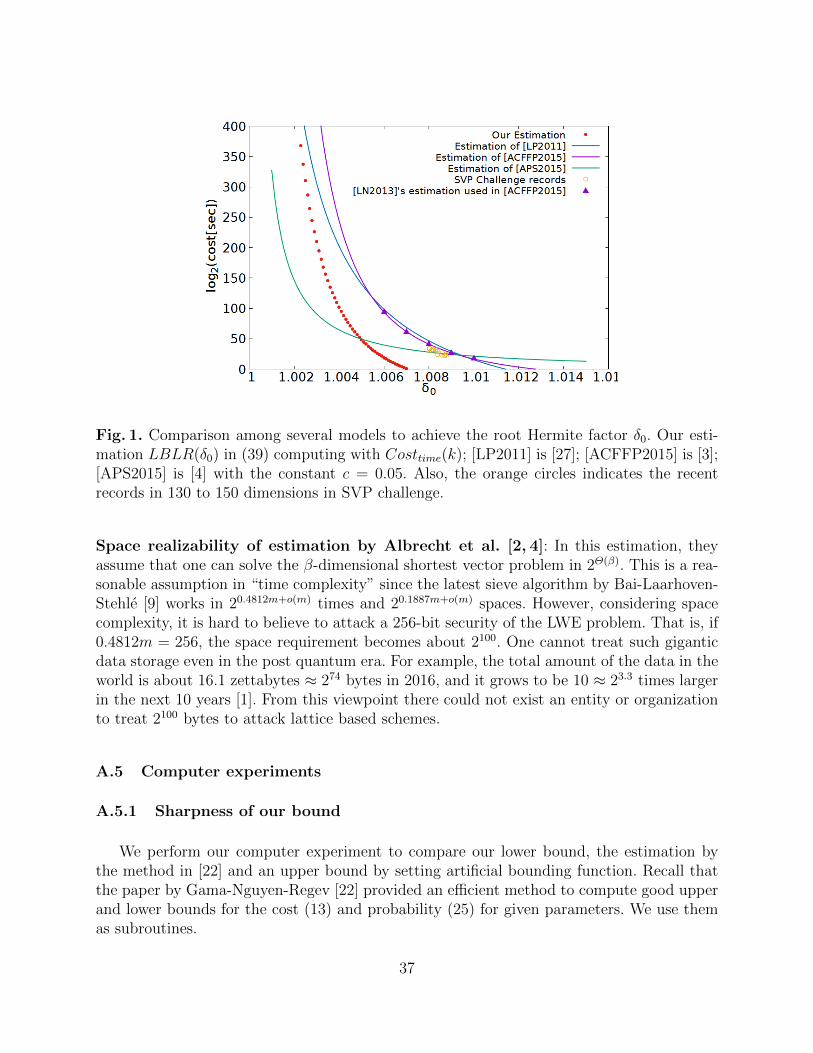
Fig. 1. Comparison among several models to achieve the root Hermite factor δ0. Our esti-mation LBLR(δ0) in (39) computing with Costtime(k); [LP2011] is [27]; [ACFFP2015] is [3];[APS2015] is [4] with the constant c = 0.05. Also, the orange circles indicates the recentrecords in 130 to 150 dimensions in SVP challenge.
Space realizability of estimation by Albrecht et al. [2, 4]: In this estimation, theyassume that one can solve the β-dimensional shortest vector problem in 2Θ(β). This is a rea-sonable assumption in “time complexity” since the latest sieve algorithm by Bai-Laarhoven-Stehle [9] works in 20.4812m+o(m) times and 20.1887m+o(m) spaces. However, considering spacecomplexity, it is hard to believe to attack a 256-bit security of the LWE problem. That is, if0.4812m = 256, the space requirement becomes about 2100. One cannot treat such giganticdata storage even in the post quantum era. For example, the total amount of the data in theworld is about 16.1 zettabytes ≈ 274 bytes in 2016, and it grows to be 10 ≈ 23.3 times largerin the next 10 years [1]. From this viewpoint there could not exist an entity or organizationto treat 2100 bytes to attack lattice based schemes.
A.5 Computer experiments
A.5.1 Sharpness of our bound
We perform our computer experiment to compare our lower bound, the estimation bythe method in [22] and an upper bound by setting artificial bounding function. Recall thatthe paper by Gama-Nguyen-Regev [22] provided an efficient method to compute good upperand lower bounds for the cost (13) and probability (25) for given parameters. We use themas subroutines.
37

Systematic Upper bound: To show the sharpness of our lower bound, and to show that oursubroutine to find ECprob,single,nodes(B; p, c) works well, we give a method to compute upperbound cost UBprob,single,nodes(B; p, c). In contrast to the lower bound situation, a possibleupper bound can be computed by setting feasible bounding coefficients. Thus, using a finiteset of bounding coefficients whose probability is larger than p, an upper bound is given bythe minimum cost among the coefficients. For this purpose, we define the pruning coefficientsin dimension m parametrized by α ∈ R and j ∈ [m] by Ri(α, j) = min((i/j)α, 1).
For given parameters (||b∗1||, . . . , ||b∗n||, c, p), and for each integer j, we can compute αso that the lower bound probability is p by the binary search. Then, by computing theminimum of upper bound cost among all j, we can obtain an upper bound of enumerationcost of probability p.
Comparison: Figure 2 shows the comparison among the systematic upper bound
UBprob,single,nodes(B; p, c),
cost of pruned enumeration ECprob,single(B; p, c), lower bound cost of single usage
LBprob,single,nodes(B; p, c)
and the lower bound for multiple usage LBprob,multi,nodes(B; p, c). We use the radius c =GH(L) and various success probability. We used two bases: a PBKZ-60 reduced 180 dimen-sional basis and a PBKZ-20 reduced 120 dimensional basis. The lattice bases are publishedinstances of SVP challenge, and PBKZ-β stands for Aono et al.’s progressive BKZ [7] withtarget blocksize β. In 180 dimension, for p < 10−4, we can see ratio
ECprob,single,nodes(B; p, c)/LBprob,single,nodes(B; p, c)
is less than 104.
A.5.2 Evidence for our Assumption 2Recall that Assumption 2 claims that
ECModel,single,Measure(B; params) ≥ LBModel,single,Measure(Bδ0 ; params)
for each Model ∈ {prob,many, LWE} and Measure ∈ {nodes, gates, time}, reasonableparameters, and δ0 = (‖b1‖/vol(L)1/m)1/m.
Figure 3 shows that the comparison among ECprob,single,node(B; p0 = 10−3, c = GH(L)),ECprob,single,node(Bδ0 ; p, c) and LBprob,single,node(Bδ0 ; p, c) for many reduced basis. We can seethe assumption holds in the all cases.
Additional experiments over several probabilities and dimensions are shown in Figure 4.These graphs show the ratios
ECprob,single(B; p0, c)
ECprob,single(Bδ0 ; p0, c)and
ECprob,single(B; p0, c)
LBprob,single(Bδ0 ; p0, c)(41)
38

Fig. 2. For two lattice bases, compare the systematic upper bound UBprob,single,nodes(B; p, c),cost of pruned enumeration ECprob,single,nodes(B; p, c), lower bound cost of single usageLBprob,single,nodes(B; p, c), and the lower bound for multiple usage LBprob,multi,nodes(B; p, c).We used a PBKZ-60 (resp. PBKZ-20) bases of random 180-dim. (resp. 120-dim) lattice.
in red and blue curves respectively. Assumption 2 claims that the right values (blue curves)always above 1. For a majority of situations, ECprob,single(B; p0, c) > ECprob,single(Bδ0 ; p0, c)holds and for all situations in our experiments, ECprob,single(B; p0, c) > LBprob,single(Bδ0 ; p0, c)holds. In the bottom-right picture, we used our version of primal-dual progressive BKZalgorithm that is a naıve combination of the primal-dual BKZ [32] and the progressiveBKZ [7].
39

Fig. 3. Comparison of various simulated costs between real reduced basis and equivalentGSA basis. (Left) 200-dimensional bases reduced by progressive BKZ [7] with many block-sizes; (Right) For LLL reduced basis of many dimensions; In all experiments, parametersare p = 10−3 and c = GH(L).
40

Fig. 4. Experiments to compare the ratios (41) for various lattice dimension m, searchingradius c, success probability p and target reduced level β of progressive BKZ. (Top-Left)Experiments using 12 bases, m = 200, c = GH(L), p = 10−3 and various β-reduced bases;(Top-Right) Experiments in using bases, c = GH(L), p = 10−3, β = 40 and various di-mensions; (Bottom-Left) Experiments using 16 bases, m = 200, c = GH(L), β = 40 andvarious success probabilities; (Bottom-Right) Experiments using 16 bases, m = 200, c =GH(L), p = 10−3. The bases are the outputs of our preliminary version of primal-dual pro-gressive BKZ.
41