Embed Size (px)
Citation preview
Max-Planck-Institut für demografische ForschungMax Planck Institute for Demographic ResearchDoberaner Strasse 114 · D-18057 Rostock · GERMANYTel +49 (0) 3 81 20 81 - 0; Fax +49 (0) 3 81 20 81 - 202; http://www.demogr.mpg.de
This working paper has been approved for release by: James W. Vaupel ([email protected])Head of the Laboratory of Survival and Longevity.
© Copyright is held by the authors.
Working papers of the Max Planck Institute for Demographic Research receive only limited review.Views or opinions expressed in working papers are attributable to the authors and do not necessarilyreflect those of the Institute.
Love and Death in Germany. The marital biography and its impact on mortality
MPIDR WORKING PAPER WP 2002-015APRIL 2002
Hilke Brockmann ([email protected]) Thomas Klein
1
Love and Death in Germany. The marital biography and its impact on mortality
by Hilke Brockmann and Thomas Klein1
Abstract
Most studies dealing with the impact of marriage on mortality treat being married as a once-
and-for-all status. However, multiple life changes in marital status characterize the modern
life course. The purpose of this paper is to analyze how the timing of these changes affect
mortality in Germany. Longitudinal data show that the positive effects of getting married
accumulate over long periods of time, while the negative effect of divorce and widowhood
attenuates after some time. We also find that the effect of any marital status wears out with an
individual’s age and differs between cohorts, which is partly due to selectivity. Both temporal
mechanism and selection processes demonstrate the plasticity of the marital biography and its
variable effect on mortality. (120 words)
1 We thank Jan Hoem for extremely helpful comments. We would also like to thank Jonathan MacGill for hispatient help with preparing the data. Conversations with Jutta Gampe and Rainer Walke have also been veryuseful. And thanks to Elizabeth Zach for polishing the English and Silvia Leek for improving the graphs. Theresearch was sponsored by and carried out at the Max Planck Institute for Demographic Research (MPIDR) inRostock, Germany.

2
Introduction
Since 1830, when Benoisten de Chateauneuf first researched the difference in life
expectancy between married and non-married persons, numerous studies have confirmed this
finding for many countries (Hu, Goldman 1990; Klein 1993; Lillard, Waite 1995; Hemström
1996; Cheung 2000). Researchers hold two distinct processes responsible for such disparities.
The first process is selection into marriage. Various studies have shown that those who find a
partner on the marriage market are healthier than those who stay alone (Goldman 1993;
Goldman, Korenman, Weinstein 1995). The second process refers to the protective
mechanism of a marriage: Being married guarantees emotional support, constrains risk-taking
behavior, stimulates a healthy life-style, provides additional resources, buffers critical
experiences and partly replaces professional health care.
Both explanations are highly plausible. But they do not capture an important element
of today’s family biographies. Men and women are much more likely today to move in and
out of different unions over the life course than they were fifty years ago. Most people live
without a partner for extensive periods of their adult lives (Settles 1999, 155). Considering
this, it is decisive to look into the timing patterns and their effect on mortality. Is being
married for 20 years twice as protective as being married for 10 years? Can married men and
women preserve their survival advantage over singles, divorcees, widowers and widows over
their whole life span? Is a marriage at the age of 40 as protective as a marriage at the age of
20? Does a marriage after a previous divorce prolong one’s life expectancy by more time
than a marriage after a previous widowhood?
The purpose of this paper is to examine, over the life course, the impact of marital
changes on mortality. There is a growing body of literature documenting that early-life events
(e.g., Barker 1998; Elo, Preston 1992; Doblhammer, Vaupel 2001) as well as mid-life

3
conditions (e.g., Manton, Stallard, & Corder 1997; Hart, Smith, & Blane 1998) are important
determinants of mortality later in life. However, all these studies focus on single life events,
and hardly ever analyze the impact of multiple event sequences. Also, they often neglect
marriage as a factor. In this paper, we trace people over long periods of time, potentially
covering multiple events, and focus on key events shaping their marital careers. Analyzing
the timing of these events should help to better understand when and why married people
have a higher life expectancy than divorced, widowed or single people. We distinguish four
different patterns of causation:
- Accumulation: Since mortality is highly correlated with age, theories of aging have
promoted the idea that the effects of negative events cumulate with time.
- Attenuation: Events do not always cumulate. Sometimes, people recover from severe
crisis. As time passes, negative influences peter out.
- Timing: Certain events may have an impact on later life only if they occur at certain
critical junctures of the life course.
- Ordering: Some events may have an impact only if they occur in a certain sequence.
For example, a divorce should be more harmful for those who stay alone than for those who
immediately move in with a new partner. By intuition, a divorce should be more harmful for
a sick than for a healthy person.
The paper is structured as follows. We first map the research background of marital
transitions and mortality differences. Next, we introduce our longitudinal data set and the
applied method, and present the empirical findings. Finally, we put our results into
perspective and conclude that a timing framework is essential for distinguishing between
path-dependent life-course effects and myopic selection effects.
4
Background
The advantageous effects of being married were first discovered in cross-sectional
data, based either on a single survey or on aggregate death registration (Gove 1973; Kobrin,
Hendershot 1977). Since the late 1970s, prospective studies are undertaken to explore the
relationship between marital status and health at baseline and mortality in the following
years. The findings from this partial panel approach confirm the health benefits and social
support of marriage even in the presence of controls for selection and socioeconomic factors
(Sorlie, Backlund, & Keller 1995; Lillard, Panis 1996; Cheung 2000).
Consistent with previous results, these later studies also demonstrate that men benefit
more from a marriage than women do. Moreover, individual differences in mortality between
divorced, widowed, single and married are larger among men than women. Depending on the
sample size, some differences turn out to be significant. Goldman et al. (Goldman,
Korenman, & Weinstein 1995) estimated from a representative sample of elderly US
Americans that widowers have about25% higher odds of dying compared to married men.
The marital status of elderly women, on the other hand, did not affect mortality. The pattern,
however, turns out to be significant when younger ages are included.
Generally, some studies show that the longevity advantage of the married tends to be
more pronounced among young and middle-age persons than among the elderly (Hu,
Goldman 1990; Korenman, Goldman 1993). However, these prospective studies consider
only baseline conditions and are unable to trace varied marriage dynamics over the whole life
span.
The significance of timing has been observed in large census-linked data, which
makes it possible to measure the consequences of marital transitions in chronological detail.
Martikainen and Valkonen (1996) have discovered excess mortality after bereavement among

5
more than 1.5 million Finns. This excess mortality is higher among men (17%) than among
women (6%). For both genders, it is highest during the first week after the death of the
spouse and drops slowly but steadily during the following 6 months.
Hemström (1996) based his study on 44,000 deaths in Sweden and analyzed the effect
of marriage dissolution on mortality. He confirms what has also been found in other countries
(Hu, Goldman 1990; Rogers 1995): a separation from one’s life-partner, particularly a
divorce, reduces one’s life expectancy. Linking several censuses with death registers, he
showed that marriage dissolution affects mortality even years after the event. However,
multiple, short- and medium-term transitions, as well as deaths that occur between censuses,
are missed.
A complete picture of the relationship between marital transitions and mortality can
only be drawn from longitudinal data. Since the 1990s, scholars analyze marital histories to
disentangle selection and protection processes over time (Zick, Smith 1991; Lillard, Waite
1995; Lillard, Panis 1996). A closer look into the dynamics of a marital biography shows that
both selection and protection processes have an effect on mortality. Furthermore, event-
history analysis makes clear that single transitions are embedded in a meaningful individual
biography, as well as in an age-graded institutionalized life course (Wunsch, Duchêne,
Thiltgès, & Sahlhi 1996).
The transition into marriage is an event from which both men and women benefit.
However, effects differ across the sexes. Men experience immediately reduced mortality risks
with marriage, and this advantage lasts through the entire life course. The transition out of
marriage –either through separation, divorce, or widowhood – immediately increases their
mortality. Women by contrast receive no immediate benefit with transition into marriage, but
survival advantages accumulate over time (Lillard, Waite 1995).
6
Furthermore, cohort and periodic timing seems to have some impact. For example,
Elder, Shanahan, and Clipp (1994) found among World War II veterans a higher risk of
divorce and a greater health decline among cohorts who entered the war after the age of 32.
And relative excess mortality of divorced persons has been shown during periods of
increased divorce rates (Mergenhagen, Lee, & Grove 1985; Trovato, Lauris 1989).
Scholars believe stress is the negative health effect of transitions out of marriage. (e.g.
Hemström 1996). It is also argued that the unmarried face generally more chronic stressors
than the married do (Pearlin, Johnson 1977). Moreover, women might encounter more stress
within a marriage than men because they have less bargaining-power and higher
expectations. For them, a divorce or widowhood might turn out to be more a relief than a
burden (Aneshensel 1992). In addition, collective experiences and secular trends may either
buffer or worsen stressful transitions.
Yet this nexus between social condition and physiological condition is assumed rather
than shown. Research on marital transitions and mortality often use stress only as a metaphor.
Data on the immediate physiological reactions to stressful marital events is lacking. However,
the way the social environment gets „under the skin“ (Taylor, Repetti 1997; Aneshensel
1992) has been shown by experimental stress research.
Endocrinologists have measured in vitro that the body immediately responds with
immune activation to physiological and psychological stressors caused by abrupt changes,
sudden events, or unexpected shocks. This is positive stress and can increase adaptive
capacities. After a short time, this activation begins to have the opposite effect. It suppresses
immunity and helps the immune system to return to baseline. At this point, stressful
experiences may not leave traces behind. It is only with major stressors of longer duration
that the immune system falls below its starting level thus qualifying it as immunosuppressing.
At this point the body becomes particularly vulnerable (Sapolsky 1998, 135p.). Repeated
7
passing through these phases of alarm, resistance, and exhaustion may elevate physiological
activity but may also cumulate damage to the organism (Selye 1956; Seeman et al. 1997).
And it also seems that the ordering of earlier experiences could compensate for later stress
(Singer, Ryff 1999).
The following paper cannot refer to physiological data, but exploits the experimental
findings. We address the marital biography as a potential source of supporting and stressful
processes, and assess their impact on mortality. To tackle the various advantageous and
deleterious influences of marital states and transitions, the analysis focuses on timing
mechanisms suggested by experimental research. We hypothesize that the effects of marital
transitions do not uniformly accumulate over time. Rather, we suspect that the effects of
certain marital transitions peter out as time goes by (attenuation), and that marital timing and
the experienced sequence of marital states (sequencing) are decisive.
Data and Method
1. Data source and sample description
Our analysis is based on the German Socio-Economic Panel Study (GSOEP) which is
held at the German Institute for Economic Research (DIW). The GSOEP is a longitudinal
household survey that provides information on individuals living in private households in
Germany (Haisken-DeNew, Frick 2000). The survey was started in Western Germany in
1984 and is conducted annually. We restrict our analysis to the West-German sample in order
to exclude both intervening social differences between the former Eastern and Western
Germany and the effect of the historical breakdown of the socialist regime. Our sample
consists of 12,484 persons, 6,019 men and 6,465 women. Between 1984 and 1998, 1,068

8
individuals participating in the survey died. Further descriptive sample statistics are displayed
in Table 1. Cases with missing information do not alter the results, even if the missing
information was interpolated and included or if all cases were excluded from the analysis.
The following results include all information.
Table 1
Graph 1 shows the survival curves of West-German men and women estimated from
our data using a simple hazard model with a constant baseline and a Gompertz age function.
We compare these estimates with the survival curves for the same cohorts in the total
population and see that our sample is fairly reliable. We may, however, have some selection
by virtue of survival or lifestyle and underestimated mortality at middle ages, particularly
among men.
Graph 1
2. Description of variables
Previous studies depend mainly on cross-sectional information. Their general
statements are based on the effect that a marital status measured at one point in time has on
subsequent mortality. These studies often implicitly assume, but fail to test, that the effects of
an advantageous or disadvantageous marital status would accumulate its effect on mortality
over time. Our analysis is based on longitudinal information that makes it possible to trace
precisely how a current marital status influences mortality and how such an influence might
9
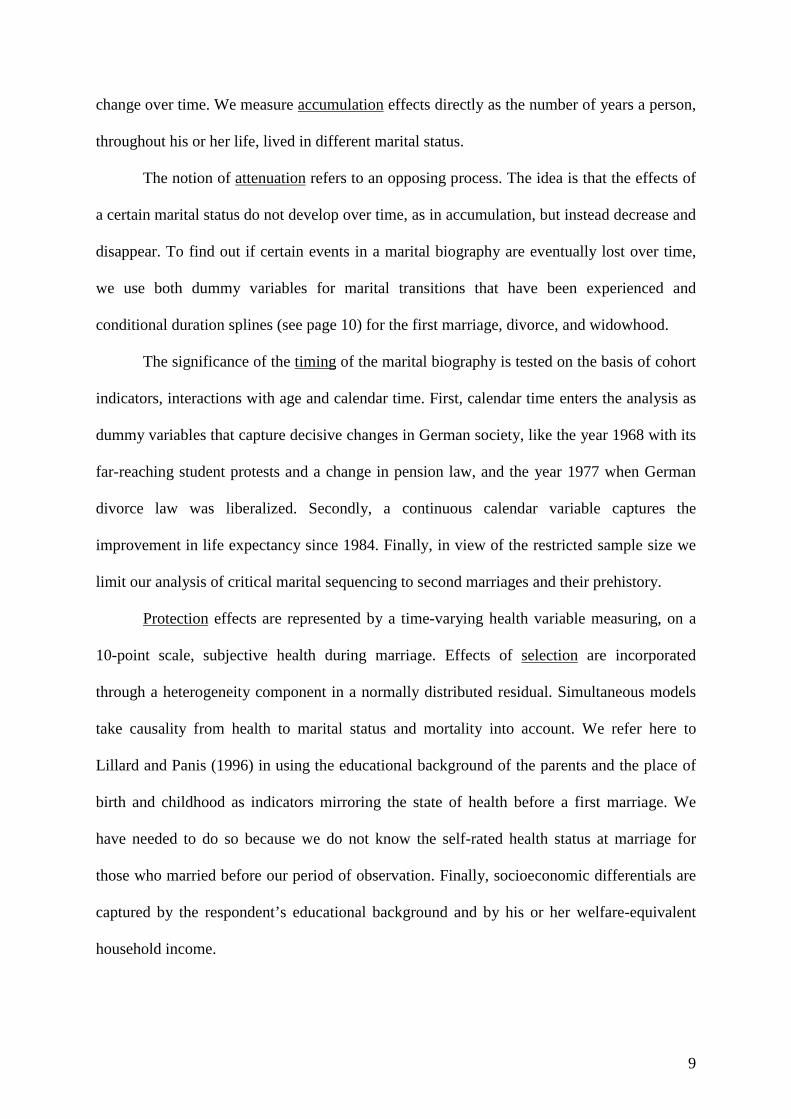
change over time. We measure accumulation effects directly as the number of years a person,
throughout his or her life, lived in different marital status.
The notion of attenuation refers to an opposing process. The idea is that the effects of
a certain marital status do not develop over time, as in accumulation, but instead decrease and
disappear. To find out if certain events in a marital biography are eventually lost over time,
we use both dummy variables for marital transitions that have been experienced and
conditional duration splines (see page 10) for the first marriage, divorce, and widowhood.
The significance of the timing of the marital biography is tested on the basis of cohort
indicators, interactions with age and calendar time. First, calendar time enters the analysis as
dummy variables that capture decisive changes in German society, like the year 1968 with its
far-reaching student protests and a change in pension law, and the year 1977 when German
divorce law was liberalized. Secondly, a continuous calendar variable captures the
improvement in life expectancy since 1984. Finally, in view of the restricted sample size we
limit our analysis of critical marital sequencing to second marriages and their prehistory.
Protection effects are represented by a time-varying health variable measuring, on a
10-point scale, subjective health during marriage. Effects of selection are incorporated
through a heterogeneity component in a normally distributed residual. Simultaneous models
take causality from health to marital status and mortality into account. We refer here to
Lillard and Panis (1996) in using the educational background of the parents and the place of
birth and childhood as indicators mirroring the state of health before a first marriage. We
have needed to do so because we do not know the self-rated health status at marriage for
those who married before our period of observation. Finally, socioeconomic differentials are
captured by the respondent’s educational background and by his or her welfare-equivalent
household income.
10
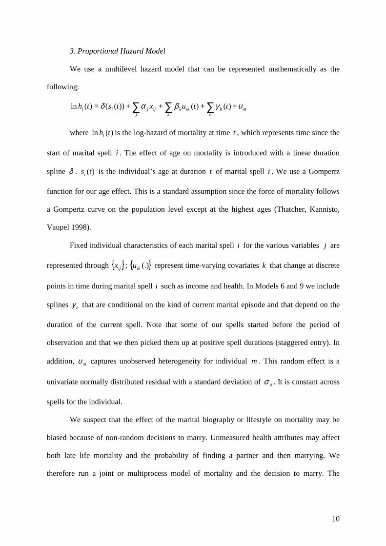
3. Proportional Hazard Model
We use a multilevel hazard model that can be represented mathematically as the
following:
∑ ∑∑ ++++=j
mh
hikk
kijjii ttuxtsth υγβαδ )()())(()(ln
where )(ln thi is the log-hazard of mortality at time t , which represents time since the
start of marital spell i . The effect of age on mortality is introduced with a linear duration
spline δ . )(tsi is the individual’s age at duration t of marital spell i . We use a Gompertz
function for our age effect. This is a standard assumption since the force of mortality follows
a Gompertz curve on the population level except at the highest ages (Thatcher, Kannisto,
Vaupel 1998).
Fixed individual characteristics of each marital spell i for the various variables j are
represented through { }ijx ; { }(.)iku represent time-varying covariates k that change at discrete
points in time during marital spell i such as income and health. In Models 6 and 9 we include
splines hγ that are conditional on the kind of current marital episode and that depend on the
duration of the current spell. Note that some of our spells started before the period of
observation and that we then picked them up at positive spell durations (staggered entry). In
addition, mυ captures unobserved heterogeneity for individual m . This random effect is a
univariate normally distributed residual with a standard deviation of υσ . It is constant across
spells for the individual.
We suspect that the effect of the marital biography or lifestyle on mortality may be
biased because of non-random decisions to marry. Unmeasured health attributes may affect
both late life mortality and the probability of finding a partner and then marrying. We
therefore run a joint or multiprocess model of mortality and the decision to marry. The
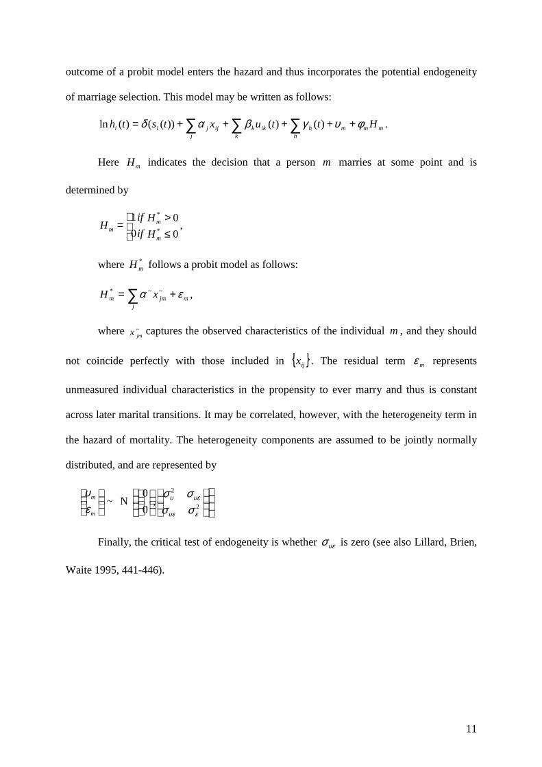
11
outcome of a probit model enters the hazard and thus incorporates the potential endogeneity
of marriage selection. This model may be written as follows:
mmj
mh
hikk
kijjii Httuxtsth φυγβαδ +++++= ∑ ∑∑ )()())(()(ln .
Here mH indicates the decision that a person m marries at some point and is
determined by
≤>
=0
0
0
1*
*
m
mm
H
H
if
ifH ,
where *mH follows a probit model as follows:
mj
jmm xH εα += ∑ ~~* ,
where ~jmx captures the observed characteristics of the individual m , and they should
not coincide perfectly with those included in { }ijx . The residual term mε represents
unmeasured individual characteristics in the propensity to ever marry and thus is constant
across later marital transitions. It may be correlated, however, with the heterogeneity term in
the hazard of mortality. The heterogeneity components are assumed to be jointly normally
distributed, and are represented by
m
m
ευ
~ N
2
2
,0
0
ευε
υευ
σσσσ
Finally, the critical test of endogeneity is whether υεσ is zero (see also Lillard, Brien,
Waite 1995, 441-446).

12
Results
1. The current status
Table 2
Model 1 in table 2 shows the gross effect of the current marital status on mortality. In
agreement with earlier findings single men have a significantly higher mortality than their
married reference group. The difference is smaller among women but, at 43 per cent, still
highly significant. A divorce shortens the life expectancy of men but not of women. In
contrast, women seem to suffer more from the death of a spouse than men do. This difference
between widows and widowers, however, vanishes when the health of the individual, his
educational background and further unmeasured characteristics summarized in a
heterogeneity factor are considered. Model 2 reveals the same detrimental effect of being
single and widowed for both men and women. It further confirms the negative impact of
being divorced on the longevity of men.
Not surprisingly, a higher subjectively rated health and a higher school education
lower mortality significantly for both sexes (model 3). Note, however, that including health
almost exclusively leads to an increasing risk to die among single women, from 43 to 67 per
cent compared to their married reference group. This suggests that there is health selection on
the female marriage market. German history may be a key to explaining this pattern. As a
consequence of World War I and II, female cohorts that contribute mainly to mortality in this
analysis are larger than their male counterparts. Therefore, these women faced high selection
pressure, whereas almost all men got married.
13
Household income indicates a further difference between the sexes. A higher income
has a positive effect on the life expectancy of women but not of men. Each thousand DM
earned lowers women’s mortality risk by 10 per cent. The traditional sex-specific division of
labor dominating among the older West-German population may explain this difference. Put
bluntly: The male breadwinner pays a price for a higher income, whereas the traditional
housewife primarily benefits from more material resources in terms of higher private
consumption. Being married does not simply stand for economic security as findings from the
United States suggest (Lillard, Waite 1995, 1144pp). On the contrary, the current marital
status remains a key explanatory factor of female mortality in West Germany, even if
heterogeneity is taken into account.
Finally, model 3 suggests that heterogeneity is only influential in the male sample.
The current marital status, health and socioeconomic factors are protective but do not explain
exhaustively the hazard of men’s mortality. The reasons may perhaps be found in their
previous biographical history.
2. The marital biography
2.1. Accumulation and attenuation
Model 4 gives a first insight into the effect of the marital biography on mortality. We
substituted the current marital status by dummy variables indicating whether a person has
never experienced a marriage or has ever experienced a divorce or the death of a spouse.
Although the information seems less meaningful than the current marital status, the
explanatory power of the model is larger. Single men face a 167 per cent higher mortality risk
than men who have been married at least once in their life. A first marriage is a better
protection for men than their current status. This difference does not exist for women.
14
Unlike the current status, whether one has ever experienced divorce or widowhood
has no significant effect on mortality in either men or women. This suggests that the impact
of negative events on mortality decline and disappear over time. Positive experiences such as
a marriage, by contrast, show an enduring protective influence.
Model 5 tests this notion in more detail. It confirms the presence of accumulation and
attenuation of marital protection. The longer men and women live in some other marital
status than single, the better their life expectancy. Women especially decrease their mortality
risk significantly the more years they remain married, divorced or widowed. The effect is
strongest for divorcees whose death risk declines by 18 per cent over ten years. But does the
force of mortality drop linearly?
Model 6 gives a first answer. Due to the sample size we introduce three splines
representing the duration of the first marriage, the first divorce segment and the first
widowhood segment. We set nodes after 7 years, in order to compare the effect of a marital
status at early and late years. As it turns out, any transition into a marriage, into a divorce or
widowhood increases the force of mortality. The stress of a new situation, even if anticipated,
may explain this shift in mortality. In addition, the reference category here includes all single
spells, men and women who never marry during their life, as well as singles who married
later. This second group adds exposure time but no events. It seems that unobserved
heterogeneity cannot absorb this selectivity completely. So, the force of mortality of the
reference category is comparatively low. However, when the clock of an episode starts
ticking, the risk of death drops immediately.
Precisely, the intercepts of the duration splines for the first marriage are highly
significant for both sexes. But for women, the effect is greater. This could be explained by
the profound change in lifestyle a woman experiences after getting married and becoming a
mother and housewife. Mortality already declines for husbands and wives during the first
15
year of their marriage. These results are not displayed here. If the first seven years are
grouped together the decline proves to be significant. The hazard of dying falls by 63 per cent
among men and 28 per cent among women2. Later years seem to be less beneficial. The
protective effect of years being married does not accumulate linearly. Rather, our results
suggest a declining marginal utility of a marriage.
Model 6 also shows a similar pattern for the duration of a divorce and widowhood.
Again, it is probably the sample size as to why these findings are not significant, except for
the intercept of a first widowhood of men and of a first divorce of women. Nevertheless, the
fit of the model, tested with a likelihood ratio test, increases significantly compared to model
5 and it left no heterogeneity in the female sample.
2.2. Timing and sequencing
Since the effect of the marital status on mortality depends on time, how do calendar
time and cohorts influence the relation of marital status and mortality? The timing of marital
transitions has turned out to be significant for many events like births or risk of a divorce, but
has not been tested for mortality. Model 7 depicts the significance of the date of the first
marriage on mortality. Men and women who got married before 1968 have a more than 50
per cent lower risk of dying than couples that married later, given that all other important
variables are controlled for.
Table 3
2 These figures result from )(exp( 1βα tn+ , where a represents the intercept of the conditional spline,
tn indicates the number of years, and 1β is the first slope estimate of the conditional spline.

16
The year 1968 marks a watershed in West-German history. The dissolution of
conventional family patterns based on the male bread-winner model accelerated. The
meaning of marriage changed. It turned from a union of two people who share the same
lifelong fate into a partnership based on love and sympathy that can be broken off at any
time. As a result, a marriage became less protective and more demanding and stressful. The
risk of death increased as compared to the earlier traditional marriage.
Moreover, birth cohorts are important. World War II reduced male cohorts drastically
and weakened survivors. This shows in their significantly higher mortality risks. Female
cohorts, by contrast, do not differ significantly. But mortality among the female population
decreases during the years of observation. A closer inspection reveals that mortality among
women declines after 1995. In that year, a new insurance for old age care had been
implemented. It is plausible that women who survive their husbands benefit from this law.
Unfortunately, we cannot test this proposition here. Finally, although the male sample
remains heterogeneous, the unobserved variance has been partly absorbed by the timing
variables.
The influence of timing carries on to individual aging. Model 8 shows that women
benefit more from any marital status. But this benefit wears out with age. For example, while
more than 74 per cent of divorced women survive up to their 60th birthday given that all other
influences are controlled for, only about 46 per cent of divorced men will likely live that
long3. This difference of nearly 30 per cent decreases, however, to 4 per cent among those 80
years old. And the trend is even stronger for widowed men and women. Finally, a 25 per cent
higher survival probability of married 60 year-old-women changes into the opposite after the
age of 87. At that point, old men are more likely to live longer than their female counterparts.
17
Graph 2
Graph 2 illustrates how age and marital status interact during the female life course.
The age variable appears as an intermediate variable that changes the significance of being
single and married as life passes. Being single is the most harmful status for women during
all their life until they become 70 years old. After the age of 70, their chances of survival are
higher than that of being widowed and, some years later also, than that of being married or
divorced. However, there seems to be not much difference left between single, married,
divorced, or widowed women in their seventies and eighties. For men, marital status and age
do not interact until late in their life. The surprisingly high survival chances of single men is a
spurious result of the small size of older male cohorts: There are only very few older men
who did not marry. By contrast, younger cohorts and men who married later in life dominate
the sample of singles and lead to an overestimation of the survival chances of single men.
Timing patterns refer to the life-course as a social institution. It is shaped by period,
cohort and aging effects that are beyond individual control. In contrast, marital transitions
express individual preferences and decisions. Their individual sequences may have an impact
on mortality. Model 9 tests this hypothesis. We restrict our analysis to second marriages that
happened after a divorce or widowhood. Both effects do not turn out to be significant,
probably because of the small sample size. However, the results point in the expected
direction. A second marriage after a divorce is more beneficial than after the death of a
spouse.
3 Given that all covariates are controlled, the baseline of the hazard model )()(ln tbathi += with intercept a
and log hazard )(tb can be translated into the survivor function: ))).exp(1()exp(/1exp()( tbabts ⋅−⋅⋅=

18
2.3. Reverse causality
Is the effect of accumulated years of being married on mortality a cause or
consequence of good health? Is the timing effect of marital transitions on mortality a cause or
a consequence? Adding heterogeneity can control for selection, but we do not know if we
control for health selection. Following Lillard and Panis (1996), we estimate a joint probit
and hazard model that brings, through marriage, health selection and health protection into
the correct chronological order.
Table 4
For men, model 10 shows that the harmful effect of remaining single is exclusively
caused by health selection into marriage. The significant gross effect on mortality of never
having been married is absorbed by the probit model which takes into account the early
health condition as a determinant of a probable marriage. The opposite seems to be true for
women. Separating the effect of selection into a marriage reveals an even higher mortality
risk for women who have never been married. This could be explained by the change in life-
style women experience due to marriage. Being a wife and mother is usually associated with
a low-risk and far-sighted way of life.
We didn’t expect that coefficients in the probit model would change when we
estimated the model jointly. This result indicates another endogeneity bias issue in the
equation. Health selection into marriage is also captured with the hazard model. So far, we
have not been able to separate early health selectivity and late life mortality completely with
data from the German Socio-Economic Panel.
Even so, the correlation between the heterogeneity component in the probit and
hazard model is significant for men in Model 10. The negative sign indicates that men who
19
have a lower than average risk to marry face a higher than average risk to die. In contrast, the
positive but not significant correlation for women may show that women with a higher than
average risk to marry face also a higher than average risk to die. Although counterintuitive at
first glance, this finding may mirror the significant interaction of marital status and age in the
female biography. Model 11 takes into account these interactions and here the correlation
������������ ���������� ���������������� ����������������������������������� ���
lower net coefficients, particularly for women. Consequently, the beneficial and harmful
effects of the marital biography are substantially understated if the health selection into a
marriage is ignored.
Discussion
(West-) Germany is no exception when it comes to love and death. The present study
confirms many results on the impact of marital status on mortality that have been found in
other countries. The marital status has a significant effect on mortality. It also seems that
West-German men benefit more from a marriage than do women. Moreover, differences in
mortality between marital status groups are larger among men than women. Also, we found
health selection on the marriage market for both sexes.
All these singular findings and single transitions are part of a meaningful individual
biography. Considering the whole life-story reveals the importance of past experiences: A
long-lasting first marriage is more protective than the current marital status; positive
transitions seem, in general, effective on a long-term basis. The impact of negative events on
life expectancy, by contrast, is often lost after a short period of time.
20
Accumulation and attenuation do not describe linear effects. Both men and women
benefit immediately from a marriage, but women benefit more than men. This finding
supports the idea of positive stress since both men and women experience a prompt change in
life-styles with their marriage. However, women undergo a more fundamental change than
their husbands, especially when they become housewives and mothers. Overtime, the
marginal utility of a first marriage declines for both partners.
Applying timing mechanisms to the calendar of the individual life course shows how
the effect of any marital status wears out with individual age. This is especially true for
women. For them, staying single is the most harmful status with respect to their longevity.
However, if they live longer than 75 years, single women do not differ from married or
divorced women and have an even lower mortality risk than widowed women. But also,
divorced men lose their survival advantage over widowed men after the age of 90. The short
of this is that the marital status changes its meaning during the life course.
Finally, each individual calendar is embedded in a social time frame. Significant
cohort effects that absorb nearly all heterogeneity in the male sample prove the direct and
indirect impact of historical events on individual mortality. The two World Wars drastically
reduced and probably weakened the health of certain male cohorts and, as a result, increased
their likelihood to find a partner and marry. The year 1968 indicates another radical change in
German society. Contraceptives, student revolts, and women’s liberation at home and on the
labor market alter the meaning of marriage and its effect on mortality. This change is more
influential than the improvement of widows’ pensions and the liberalization of the divorce
law in 1977.
What follows from these results? First, the analysis of marital status and mortality has
to go back to the individual biography. Accumulation and attenuation represent simple
mechanisms that structure the biographical time horizon. The accumulation of positive
21
experiences somewhat contradicts the general notion of aging. Aging is often equated with an
accumulation of negative events and frailty. By comparison, our finding points to the wealth
of experiences that older people possess and which may prolong their life. The attenuation of
negative events on the other hand undermines what life-course research has promoted: a
lifelong mode of action and path-dependency. Our findings show a less deterministic
connection between negative earlier events and later mortality. Attenuated effects also
suggest that life course research overestimate the significance of biographical continuity.
What appears to be a detrimental biographical effect may be a selection effect. It is important
to distinguish between both. This brings us to a second conclusion.
Cohort and period effects as well as interactions with age prove the importance of
timing. The timing of a marital transition and its effect on mortality refer to different
selection processes. The mortality disadvantage for younger single women i.e. that converts
partly into an advantage after the age of 75 can be explained either biologically by the earlier
deaths of frail singles or socially by the shift in majorities. Most women are single at that age.
They may establish new support-networks or benefit from the same institutional help more
easily than older widowed or divorced women do. The latter argument seems most plausible
since interactions that have been found for women do not exist for men. For men, cohort
effects translate into low selection pressure on the marriage market and absorb heterogeneity
to a large extend in the sample. The significant period effect, we found, indicates the change
of a marriage as a social institution. The liberalization of private ways of living goes hand in
glove with new selection rules. Having strong affections for somebody does not necessarily
describe a stable condition that is good for one’s health.
Both, temporal mechanism and social selection processes demonstrate the plasticity of
the marital biography and its effect on mortality.

22
References
Aneshensel, C.S. (1992) Social Stress: theory and research. Annual Review of Sociology 18,
15-38.
Barker, D.J.P. (1998) Mothers, babies and health in later life. Edinburgh: Churchill
Livingstone.
Cheung, Y.B. (2000) Marital status and mortality in British women: a longitudinal study.
International Journal of Epidemiology 29, 93-99.
Doblhammer, G., Vaupel, J.W. (2001) Life span depends on month of birth. Proceedings of
the National Academy of Sciences of the United States of America 98, 2934-2939.
Dohrenwind, B.P., Dohrenwind, B.S. (1976) Sex differences and psychiatric disorders.
American Journal of Sociology 81, 1447-1454.
Elder, G.H., Shanahan, M.J., Clipp, E.C. (1994) When war comes to men’s lives: life-course
patterns in family, work, and health. Psychology and Aging 9, 5-16.
Elo, I.T, Preston, S. (1992) Effects of early life conditions on adult mortality. Population
Index 58, 186-212.
Goldman, N. (1993) Marriage selection and mortality patterns: Inferences and fallacies.
Demography 30, 189-208.
Goldman, N., Hu, Y. (1993) Excess Mortality among the Unmarried: A Case Study of Japan.
Social Science & Medicine 36, 533-546
Goldman, N., Korenman, S., Weinstein, R. (1995) Marital status and health among the
elderly. Social Sciences & Medicine 40, 1717-1730.
Gove, W.R. (1973) Sex, Marital status, and mortality. American Journal of Sociology 79, 45-
67.
Haisken-DeNew, J.P., Frick, J.R. (eds) (2000) Desktop Companion to the German Socio-
Economic Panel Study. DIW, Berlin.
http://www.diw.de/deutsch/sop/service/dtc/index.html
Hart, C.L., Smith, G.D., Blane, D. (1998) Inequalities in mortality by social class measured at
3 stages of the life-course. American Journal of Public Health 88, 471-474.
Hemström, Ö. (1996) Is marriage dissolution linked to differences in mortality risks for men
and women? Journal of Marriage and the Family 58, 366-378.
Hu, Y., Goldman, N. (1990) Mortality differentials by marital status: An international
comparison. Demography 27, 233-250.

23
Kessler, R.C. (1979) Stress, social status, and psychological distress. Journal of Health &
Social Behavior 20, 259-272.
Klein, T. (1993) Soziale Determinanten der Lebenserwartung. Kölner Zeitschrift für
Soziologie und Sozialpsychologie 45, 712-730.
Kobrin, F.E., Hendershot, G.E. (1977) Do family ties reduce mortality? Evidence from the
United States, 1966-1968. Journal of Marriage and the Family 39, 737-745.
Korenman, S., Goldman, N. (1993) Health and mortality differentials by marital status at
older ages: economics and gender. Working paper No. 93-8. Office of Population
Research, Princeton, NJ.
Lillard, L.A., Brien, M.J., Waite, L.J. (1995) Premarital cohabitation and subsequent marital
dissolution: a matter of self-selection? Demography 32, 437-457.
Lillard, L.A., Waite, L.J. (1995) Til death do us part: marital disruption and mortality.
American Journal of Sociology 100, 1131-1156.
Lillard, L.A., Panis, C.W.A. (1996) Marital status and mortality: the role of health.
Demography 33, 313-327.
Manton, K.G., Stallard, E., Corder, L. (1997) Changes in the age dependence of mortality and
disability: cohort and other determinants. Demography 34, 135-157.
Martikainen, P., Valkonen, T. (1996) Mortality after death of spouse in relation to duration of
bereavement in Finland. Journal of Epidemiology and Community Health 50, 264-
268.
Mergenhagen, P.M., Lee, B.A., Grove, W.R. (1985) Til death do us part: recent changes in
the relationship between marital status and mortality. Sociology & Social Research
70, 53-56.
Pearlin, L.I., Johnson, J.S. (1977) Marital status, life-strains and depression. American
Sociological Review 42, 704-715.
Rogers, R.G. (1995) Marriage, sex, and mortality. Journal of Marriage and the Family 57,
515-526.
Sapolsky, R.M. (1998) Why zebras don’t get ulcers: a guide to stress, stress-related diseases
and coping. New York: Freeman.
Seeman, T.E., Singer, B.H., Rowe, J.W., Horwitz, R.I., McEwen, B.S. (1997) Price of
adaptation-allostatic load and its health consequences. Archives of Internal Medicine
157, 2259-2268.
Selye, H. (1956) The stress of life. New York: McGraw-Hill.
24
Settles, B.H. (1999) The Future of families. In M.B. Sussman, S.K. Steinmetz, G.W. Peterson
(Eds.) Handbook on marriage and the family. (2nd ed) (pp. 143-176). New York:
Plenum.
Singer, B., Ryff, C.D. (1999) Hierarchies of life histories and associated health risks. Annals
of the New York Academy of Sciences 896, 96-115.
Sorlie, P.D., Backlund, E., Keller, J.B. (1995) US mortality by economic, demographic, and
social characteristics: The National Longitudinal Mortality Study. American Journal
of Public Health 85, 949-956.
Taylor, S.E., Repetti, R.L., Seeman, T. (1997) Health psychology: what is an unhealthy
environment and how does it get under the skin? Annual Review of Psychology 48,
411-447.
Thatcher, A.R., Kannisto, V., Vaupel, J.W. (1998) The force of mortality at ages 80 to 120.
Monographs of Population Aging 5, Odense: Odense University Press.
Trovato, F., Lauris, G. (1989) Marital status and mortality in Canada. Journal of Marriage
and the Family 51, 907-922.
Turner, R.J., Wheaton, B., Lloyd, D.A. (1995) The epidemiology of social stress. American
Sociological Review 60, 104-125.
Wunsch, G., Duchêne, J., Thiltgès, E., Sahlhi, M. (1996) Socio-Economic Differences in
Mortality. A life course approach. European Journal of Population 12, 167-185.
Zick, C.D., Smith, K.R. (1991) Marital transitions, poverty, and gender differences in
mortality. Journal of Marriage and the Family 53, 327-336.

Graph 1: Survival curves of West-German cohorts, GSOEP and total population
0
20
40
60
80
100
20 30 40 50 60 70 80 90Age
%men
women
male pop
female pop

Graph 2: Survival curves by marital status
Men:
Women:
0
20
40
60
80
100
20 30 40 50 60 70 80 90Age
%single
married
divorced
widowed
0
20
40
60
80
100
20 30 40 50 60 70 80 90Age
%
single
married
divorced
widowed
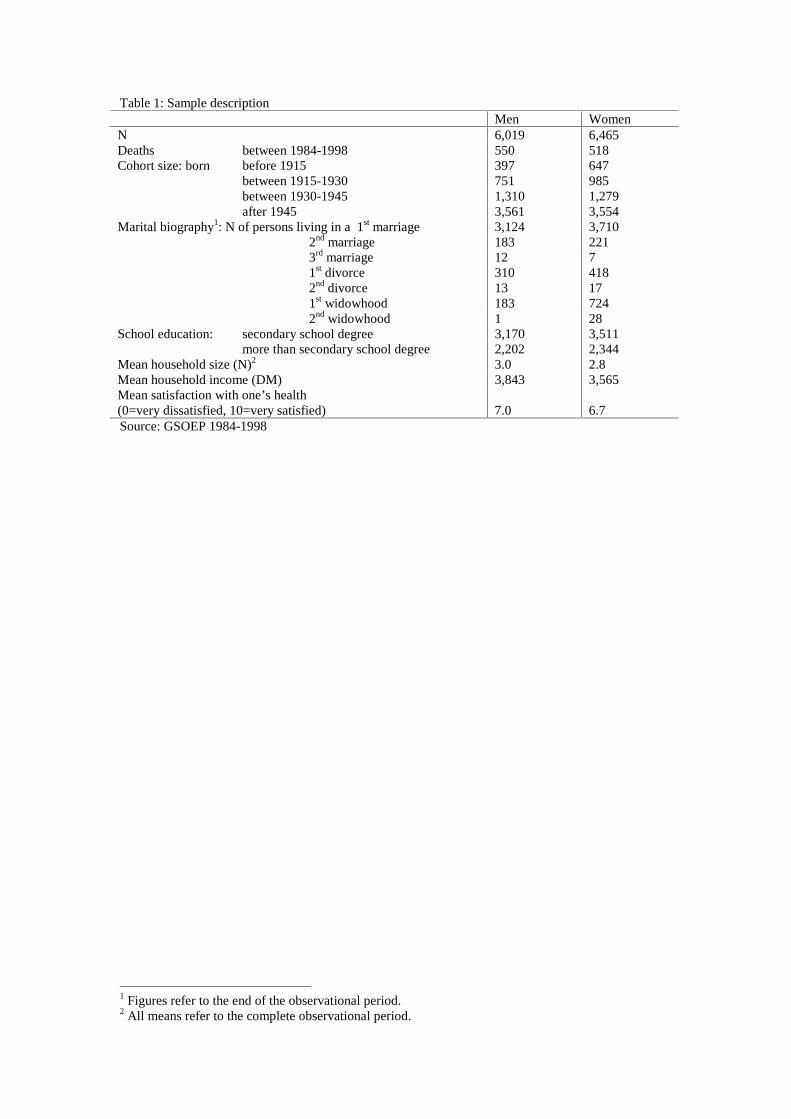
Table 1: Sample descriptionMen Women
N 6,019 6,465Deaths between 1984-1998 550 518Cohort size: born before 1915 397 647
between 1915-1930 751 985between 1930-1945 1,310 1,279after 1945 3,561 3,554
Marital biography1: N of persons living in a 1st marriage 3,124 3,7102nd marriage 183 2213rd marriage 12 71st divorce 310 4182nd divorce 13 171st widowhood 183 7242nd widowhood 1 28
School education: secondary school degree 3,170 3,511more than secondary school degree 2,202 2,344
Mean household size (N)2 3.0 2.8Mean household income (DM) 3,843 3,565Mean satisfaction with one’s health(0=very dissatisfied, 10=very satisfied) 7.0 6.7Source: GSOEP 1984-1998
1 Figures refer to the end of the observational period.2 All means refer to the complete observational period.

Table 2: Accumulated and deleted effects of marital transitions on mortalityMen WomenModel 1 Model 2 Model 3 Model 4 Model 5 Model 6 Model 1 Model 2 Model 3 Model 4 Model 5 Model 6
ge slope (in years) 1 0.096(***) 0.090(***) 0.090 (***) 0.096 (***) 0.106 (***) 0.094 (***) 0.098(***) 0.084 (***) 0.083(***) 0.090(***) 0.0967(***) 0.089 (***)
onstant -10.204(***) -8.635(***) -8.531(***) -8.929 (***) -8.764 (***) -7.990 (***) -10.987(***) -8.756 (***) -8.449(***) -8.685(***) -8.697(***) -8.374(***)
arital status:Currently single 1.584(***) 1.628(**) 1.634(**) 1.428(**) 1.562 (***) 1.665(***)
divorced 1.510(*) 1.577(*) 1.555(*) 1.038 0.892 0.966
widowed 1.190 1.378(**) 1.353(**) 1.377(***) 1.369 (***) 1.350(**)
never been married 2.671 (***) 1.667(***)
ever been divorced 1.183 0.749
widowed 0.843 0.860
Divorced/widowed 0.992 1.191
ccumulated years (in tens of years)ever been married 0.784 (***) 0.860(***)
divorced 1.001 0.819(**)
widowed 0.967 0.924(**)
onditional splines:Years of 1st marriage
intercept 1.237 (***) 1.506 (***)
0-7 -0.317 (***) -0.262 (***)
7+ 0.001 -0.006
Years of 1st divorceintercept 0.617 1.029
0-7 -0.063 -0.202
7+ 0.006 0.008
Years of 1st widowhoodintercept 0.473 (*) 0.414 (*)
0-7 -0.053 -0.015
7+ 0.001 -0.002
ealth 0.777(***) 0.780 (***) 0.781 (***) 0.779 (***) 0.781 (***) 0.751 (***) 0.756(***) 0.756(***) 0.755(***) 0.760 (***)
igher income2 (in thousands of DM) 1.010 1.026 1.022 1.020 0.900(***) 0.898(***) 0.905(***) 0.925 (**)
igher school education3 0.731 (***) 0.720 (***) 0.738 (***) 0.741 (***) 0.741(**) 0.729(**) 0.710(***) 0.737 (**)
eterogeneity υσ 1.745(***) 1.700 (***) 1.712 (***) 1.647 (***) 1.632 (***) 1.467 (*) 1.411 1.415 1.505(**) 1.272
erson-years 63,106 63,106 63,106 63,106 63,106 63,106 68,251 68,251 68,251 68,251 68,251 68,251
vents 550 550 550 550 550 550 518 518 518 518 518 518
og-likelihood -2,416.67 -2,300.24 -2,295.92 -2,284.67 -2,275.52 -2,256.16 -2,300.61 -2,165.56 -2,159.11 -2,153.92 -2,148.87 -2,139.15
Significance: *=10%, **=5%, ***=1%
1��������������� ������������ ������������� ���� ���������������� ����� ��� ������������������� ������������������������ ��������� ������������ ��������� �� �������� �standard deviations.2 Household income is displayed as welfare equivalent household income3 Higher school education stands for more than secondary school degree Source: GSOEP 1984-1998

Table 3: Timing and sequencing effects of marital transitions on mortalityMen1 WomenModel 7 Model 8 Model 9 Model 7 Model 8 Model 9
Age slope (in years)2 0.078(***) 0.097(***)
Constant -8.496(***) -9.029(***)
Date of 1st marriage before 1968 0.457(***) 0.397(***) 0.396(***) 0.427(***) 0.323(***) 0.327(***)
Date of 1st divorce before 1977 1.338 1.966
Date of 1st widowhood before 1968 0.983 0.725
Interactions:Intercept currently single -7.755(***) -7.745(***) -7.995(***) -7.990(***)
Age * single 0.057(***) 0.057(***) 0.079(***) 0.079(***)
Intercept currently married -8.044(***) -8.083(***) -9.413(***) -9.409(***)
Age * married 0.084(***) 0.084(***) 0.102(***) 0.102(***)
Intercept currently divorced -7.562(***) -7.591(***) -10.123(***) -10.095(***)
Age * divorced 0.080(***) 0.080(***) 0.112(***) 0.111(***)
Intercept currently widowed -6.810(***) -6.797(***) -9.829(***) -9.784(***)
Age * widowed 0.070(***) 0.070(***) 0.110(***) 0.109(***)
Conditional splines:Intercept 2nd marriageafter a divorce 0.045 -0.280
Slope 2nd marriageafter a divorce 0.011 0.008
Intercept 2nd marriage afterwidowhood -0.057 0.108
Slope 2nd marriage after widowhood -0.014 -0.010
Cohorts born before 1915 3.248(***) 2.590 (**) 2.667(**) 0.958 0.792 0.792
between 1915-1925 2.509(***) 2.272 (**) 2.281(**) 0.874 0.820 0.819
1925-1935 2.741(***) 2.682(***) 2.696(***) 1.022 1.110 1.098
Calendar time since 1984 0.992 0.988 0.989 0.956(***) 2.2143(***) 2.213 (***)
Heterogeneity υσ 1.497(**) 1.345 1.355(*) 1.180 1.521 (*) 1.499(*)
Person-years 63,106 63,106 63,106 68,251 68,251 68,251
Events 550 550 550 518 518 518
Log-likelihood -2,252.88 -2,246.75 -2,244.82 -2,132.64 -2,122.45 -2,121.60
Significance: *=10%, **=5%, ***=1%; Source: GSOEP 1984-1998
1 All models account for health, income, and school education. Model 7 and model 9 control also for accumulated years ever been married, divorced, and widowed.2��������������� ������������ ������������������������ ���� ���������������� ����� ��� ������������ ������������������������ ��3 The continuous year variable has been exchanged by a dummy variable differentiating between the time before and after 1995. Reference category are the years 1995 andlater.
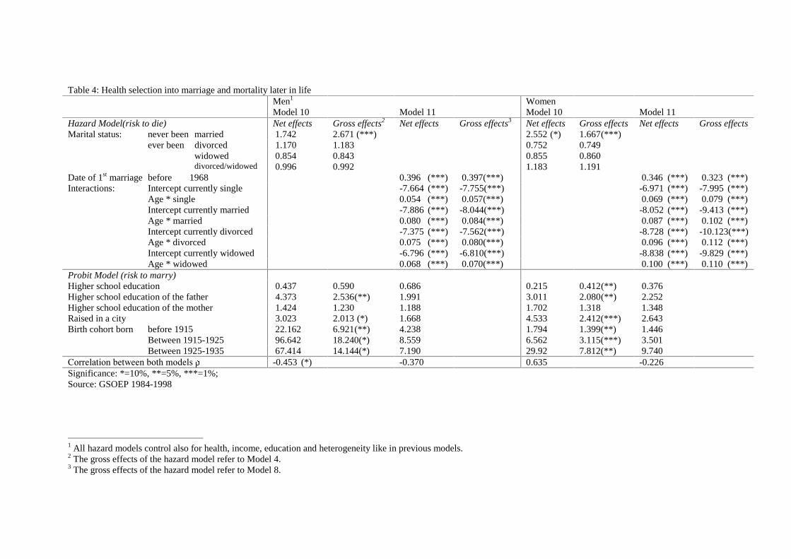
Table 4: Health selection into marriage and mortality later in lifeMen1 WomenModel 10 Model 11 Model 10 Model 11
Hazard Model(risk to die) Net effects Gross effects2 Net effects Gross effects3 Net effects Gross effects Net effects Gross effectsMarital status: never been married 1.742 2.671 (***) 2.552 (*) 1.667(***)
ever been divorced 1.170 1.183 0.752 0.749widowed 0.854 0.843 0.855 0.860divorced/widowed 0.996 0.992 1.183 1.191
Date of 1st marriage before 1968 0.396 (***) 0.397(***) 0.346 (***) 0.323 (***)Interactions: Intercept currently single -7.664 (***) -7.755(***) -6.971 (***) -7.995 (***)
Age * single 0.054 (***) 0.057(***) 0.069 (***) 0.079 (***)Intercept currently married -7.886 (***) -8.044(***) -8.052 (***) -9.413 (***)Age * married 0.080 (***) 0.084(***) 0.087 (***) 0.102 (***)Intercept currently divorced -7.375 (***) -7.562(***) -8.728 (***) -10.123(***)Age * divorced 0.075 (***) 0.080(***) 0.096 (***) 0.112 (***)Intercept currently widowed -6.796 (***) -6.810(***) -8.838 (***) -9.829 (***)Age * widowed 0.068 (***) 0.070(***) 0.100 (***) 0.110 (***)
Probit Model (risk to marry)Higher school education 0.437 0.590 0.686 0.215 0.412(**) 0.376Higher school education of the father 4.373 2.536(**) 1.991 3.011 2.080(**) 2.252Higher school education of the mother 1.424 1.230 1.188 1.702 1.318 1.348Raised in a city 3.023 2.013 (*) 1.668 4.533 2.412(***) 2.643Birth cohort born before 1915 22.162 6.921(**) 4.238 1.794 1.399(**) 1.446
Between 1915-1925 96.642 18.240(*) 8.559 6.562 3.115(***) 3.501Between 1925-1935 67.414 14.144(*) 7.190 29.92 7.812(**) 9.740
������������������� ������ -0.453 (*) -0.370 0.635 -0.226Significance: *=10%, **=5%, ***=1%;Source: GSOEP 1984-1998
1 All hazard models control also for health, income, education and heterogeneity like in previous models.2 The gross effects of the hazard model refer to Model 4.3 The gross effects of the hazard model refer to Model 8.