Love wave dispersion in central North America determined ... pubs... · Love wave dispersion in central North America determined using absolute displacement seismograms from high-rate

Love wave dispersion in central North America determined

using absolute displacement seismograms from high-rate GPS

James P. Davis1 and Robert Smalley Jr.1

Received 31 December 2008; revised 6 July 2009; accepted 28 July 2009; published 3 November 2009.

[1] We use seismic array processing of high-rate GPS (HRGPS) displacement time seriesfrom the Great, 2004, Mw 9+, Sumatra-Andaman earthquake recorded at over 90nonuniformly distributed HRGPS stations in central North America to determine thefundamental Love wave phase velocity dispersion curve there. These measurements wereperformed using frequency domain beam forming, which we show reduces the effects ofGPS multipath and common mode noise on the measurement of surface wave phasevelocity and azimuth. Our HRGPS based results for surface wave phase velocity agreewell with those obtained from 28 broadband seismometers between periods of 20 to 300 s.By separating waves based on their apparent velocity, beam forming supports the simplemodel for relative displacement HRGPS time series as being the difference betweenthe reference and kinematic station’s absolute displacements. Beam forming alsodemonstrates that for differential GPS processing the infinite apparent velocity beam of anarray is composed of the sum of common mode noise and the reference station’s absolutedisplacements, multipath and noise. We show the infinite apparent velocity beam, whichwe call the generalized spatial filter, is similar to the spatial filter commonly used toremove common mode noise from HRGPS seismograms and can be used to produceabsolute displacement time series for the kinematic stations with reduced common modenoise. Beam forming also suggests a filtering method, complimentary to sidereal filtering,to produce GPS multipath reduced HRGPS time series.

Citation: Davis, J. P., and R. Smalley Jr. (2009), Love wave dispersion in central North America determined using absolute

displacement seismograms from high-rate GPS, J. Geophys. Res., 114, B11303, doi:10.1029/2009JB006288.

1. Introduction

[2] We apply seismic array processing analysis techni-ques to high-rate GPS (HRGPS) displacement time series tomeasure surface wave dispersion and investigate how arrayprocessing can improve HRGPS displacement seismo-grams. One significant result is that the spatial filter method,developed to remove common mode noise, can be general-ized to also remove the reference station’s contribution fromdifferential GPS displacements to produce absolute GPSdisplacements. This is because the generalized spatial filterwe introduce contains everything that is common mode,which beam forming demonstrates also includes the refer-ence station’s displacements, multipath and noise. Remov-ing the common mode signal is not required when beamforming, as the common mode signal is naturally separatedfrom other signals. Removing the common mode and beamforming the resulting absolute displacement time series,however, improves the signal-to-noise ratio for the seismicwaves and facilitates automating the measurement of phasevelocity and azimuth.

[3] Traditional GPS phase data is recorded at 30 s epochsand produces millimeter precision daily positions for tec-tonic and other applications [e.g., Bock et al., 1986]. Thecontinuously increasing number of geophysical observationtypes from these GPS data include: long-term secular platemotions [e.g., Sella et al., 2002], and interseismic loading[Kreemer et al., 2003], coseismic and postseismic faultmovements [e.g., Hudnut et al., 1994], details of activedeformation associated with ongoing orogeny [e.g., Brookset al., 2003], aseismic slip or slow earthquakes from anumber of tectonic environments [e.g., Dragert et al.,2001], and nonsecular vertical loading from a variety ofsources with periods of weeks to years [e.g., vanDam et al.,1994a].[4] As GPS technology and analysis techniques improved,

it became possible to obtain displacements at each GPSmeasurement epoch with precision between 1 and 2 mm anda centimeter using kinematic processing [vanDam et al.,1994b; Hatanaka et al., 1994], instantaneous positioning[Bock et al., 2000], differential processing [Herring, 2009a;Larson et al., 2003], or precise point positioning (PPP)[Kouba, 2003]. PPP, which produces absolute positionusing a single GPS station, is currently less precise thanthe other methods, which use some form of differential orrelative positioning between two or more stations.[5] Relative displacement time series from the MW 7.1,

1999, Hector Mine earthquake [Nikolaidis et al., 2001],

JOURNAL OF GEOPHYSICAL RESEARCH, VOL. 114, B11303, doi:10.1029/2009JB006288, 2009ClickHere

for

FullArticle

1Center for Earthquake Research and Information, University ofMemphis, Memphis, Tennessee, USA.

Copyright 2009 by the American Geophysical Union.0148-0227/09/2009JB006288$09.00

B11303 1 of 19

http://dx.doi.org/10.1029/2009JB006288

produced using instantaneous positioning, clearly showdisplacements associated with the surface waves. Nikolaidiset al. [2001] used 30 s data and short baselines, 10–30 km,for sites between 50 and 200 km epicentral distance.Because the time series are aliased, as noted by Nikolaidiset al. [2001], they cannot provide meaningful informationabout either their time history or spectral content of theground motion. In the epicentral region of moderate andlarger earthquakes, Fourier components of ground motionwith periods less than 1 min, the Nyquist limit for 30 ssampling, can have amplitudes of order cm or greater andfaster data collection rates are needed to properly recordsuch signals.[6] Until recently, the paucity of HRGPS stations severely

limited their use because the most precise processing, whichproduces relative positions, requires all the data used in theanalysis to be collected at the same rate. The 2002, Denaliearthquake was the first that was widely recorded at 1 Hz,and Larson et al. [2003] found displacements of kinematicstations in the epicentral area with respect to a distantreference station in Colorado. The reference station inColorado was assumed to be stationary, which was trueuntil the seismic surface waves arrived in Colorado wherethey were large enough to affect the GPS measurements.Before the surface waves arrived in Colorado, therefore, therelative displacement time series practically representedabsolute displacements in Alaska since the station in Colo-rado was stationary. By the time the surface waves arrivedin Colorado, seismic motion had died down in the epicentralarea in Alaska, so the relative displacement time series thenrepresented absolute displacements in Colorado. Absolutedisplacement surface waves from Denali were observed byHRGPS to distances of almost 4000 km by using longbaselines and selecting the reference station such that it wasnot simultaneously affected by seismic waves.[7] Using the instantaneous positioning method over

short baselines in a small aperture network of four 1 HzHRGPS stations in southern California, Bock et al. [2004]also observed surface waves from the Denali earthquake atan epicentral distance of 3900 km. Since the referencestation in this case was also being simultaneously affectedby the seismic waves the HRGPS time series representedrelative displacements. Interpretation of relative displace-ment time series is problematic as these time series do notrepresent the motion due to the seismic waves at any singleHRGPS station. Bock et al. [2004] compared sidereallyfiltered 1 Hz HRGPS displacement time series, both beforeand after spatial filtering, to absolute displacement seismo-grams from nearby broadband seismometers and found bothagreed well at periods longer than 1 s, with better agreementfor the spatially filtered data. We will show later that thespatially filtered time series in this case were actuallyabsolute displacements.[8] Since the Denali earthquake, HRGPS applications

have also observed a wider range of large amplitude, weakmotion, surface waves [Ohta et al., 2006; Takasu, 2006] andcaptured near field coseismic offset and strong motiondisplacement time series that have been used independentlyor together with seismic data to invert for fault slip [Larsonet al., 2003; Ji et al., 2004; Miyazaki et al., 2004; Kobayshiet al., 2006; Emore et al., 2007]. Visually, HRGPS datafrom epicentral areas compares well with integrated strong

motion data [Ji et al., 2004; Miyazaki et al., 2004; Bock etal., 2004], but the question of sampling rates required toprevent temporal aliasing of very near field coseismicdisplacements using HRGPS data has not been properlyaddressed. Integration of strong motion records at epicentraldistances of <5 km from M > 6 earthquakes, for example,shows that 1 Hz data there can be significantly aliased(Smalley, in revision). This is a pure signal processingconsideration, as the signal being recorded, including anypreconditioning antialias filtering that can be applied tolimit the bandwidth, is the determining factor here, not thecapability of the GPS receiver to track the GPS signal.[9] The Great, 2004, Mw 9+, Sumatra-Andaman earth-

quake produced the first opportunity to apply HRGPSseismology on a global scale. This earthquake generatedseismic waves of enormous amplitudes that clipped a largefraction of seismic recording systems globally. SparseHRGPS data resolved strains of 6 � 10�6 and recordeddisplacements of 5–10 cm amplitude from surface waves at2500–3000 km distance [Ohta et al., 2006]. Absolutedisplacement time series were obtained for HRGPS stationson Diego Garcia and Jakarta at 2000 to 2500 km epicentraldistance using differential processing and reference HRGPSstations in Kenya and Japan at over 6000 km epicentraldistance [Ohta et al., 2006]. The surface waves took �10min to arrive at the kinematic stations and �25 min to arriveat the reference stations. This time difference left an �15min window in which absolute displacements could befound using differential processing. The distance betweenthe stations being affected by the seismic waves and thereference station, which is restricted to being outside thearea affected by the seismic waves, is limited by thedifferential processing requirement that all stations see aset of common satellites. This condition limits the distancebetween the reference and nonreference stations, whichrestricts the time window available to obtain absolutedisplacements. For an earthquake as large as the Sumatra-Andaman event, which affected the whole earth, the con-ditions on the reference station make it difficult to obtainabsolute displacement time series during the time range overwhich surface waves pass by a given location.[10] Using PPP, which produces absolute displacements

for a single station, Takasu [2006] reported detection ofabsolute displacements associated with surface waves fromthe earthquake to a distance of 13,000 km, which is less thanthe distance at which they can be both observed and analyzedwith relative positioning. In addition to the dynamic, tran-sient seismic waves, the earthquake also produced a staticcoseismic displacement field that was measured using GPS.Ohta et al. [2006] were unable to observe any suchdisplacement from integration of the HRGPS displacementdata, but Kreemer et al. [2006], using standard dailyprocessing, found �4 mm of coseismic offset for the GPSstation on Diego Garcia and coseismic offsets that are atleast 1mm in magnitude globally.

2. Sumatra-Andaman Seismic Waves in CentralNorth America

[11] The back azimuth to the Sumatra-Andaman earth-quake from central North America (CNA) is �N, whichresults in the seismic waves being naturally polarized in the

B11303 DAVIS AND SMALLEY: LOVE WAVE DISPERSION FROM HIGH-RATE GPS

2 of 19

B11303

geographic coordinate system used by both GPS andseismology. The �N-S strike of the fault and the �westdirected thrusting also place CNA in the maximum andminima, respectively, of the Love and Rayleigh wave radi-ation patterns. Love waves, with periods >60 s and peak-to-peak displacement amplitudes >4 cm, were well recordedby broadband seismometers in CNA at epicentral distancesof over 14,000 km. Displacements this large should beeasily measurable with GPS. At the time of the Sumatra-Andaman earthquake, two 1 Hz HRGPS stations (PTGVand MACC) of the GPS Array for Mid-America (GAMA)were operating in the New Madrid seismic zone of centralNorth America (Figure 1). We used the TRACK kinematicGPS processing module [Chen, 1998; Herring, 2009b,2009c] of the GAMIT/GLOBK package [King and Bock,2000; Herring, 2009a] to produce kinematic HRGPS rela-tive displacement time series in which Love waves areclearly observed (Figure 2, middle).

[12] The two GAMA HRGPS stations are approximatelycollocated with two broadband seismic stations, PVMO andFVM, respectively, of the Cooperative New Madrid SeismicNetwork (Figure 1). HRGPS station PTGV is �5 m fromthe broadband seismometer PVMO, while HRGPS stationMACC is �15 km along raypath distance from the broad-band seismometer FVM. The MACC to FVM spacing ismuch less than a seismic wavelength for waves with aperiod greater than about 20 s, and we will consider themcollocated. Since both HRGPS stations were simultaneouslyaffected by the surface waves, the kinematic GPS analysisproduces a single time series of the relative positionbetween the two stations rather than a time series ofabsolute positions for each. To compare the HRGPS relativedisplacement time series to the broadband seismometerdata, we calculated a relative displacement seismogramusing data from the two seismic stations. As the broadbandseismometers record velocity, we removed the instrument

Figure 1. Map of HRGPS (open triangles) and broadband seismometers (gray triangles) used in thisanalysis (except one HRGPS station far to the north in Canada, CHUR, and one far to the south inBogota, BOGT). HRGPS stations PTGV (bold gray triangle) and MACC (star) are approximatelycolocated with broadband seismometers PVMO and FCM, respectively (all labeled). PTGV and MACCare on stable geodetic monuments designed for tectonic studies. The dense groups of HRGPS stations arenetworks operated by the states of Michigan, Ohio and North Carolina, while the more disperse stationsare mostly from the U.S. Continuously Operating Reference Stations (CORS) and the Federal AviationAdministration (FAA) networks. These networks were built to support surveying activity or airnavigation, and most of the antenna monuments are less stable than those installed for scientific studies.During the several hour period of interest of this study, however, these monuments are sufficiently stable.


3 of 19

B11303

Figure

2.

Comparisonofrelativedisplacementseismogramsfrom

apairofapproxim

atelycollocatedHRGPS(PTGVand

MACC)andbroadbandseismometers(PVMO

andFVM).

(See

Figure

1forstationlocations.)(top)Trace

isrelative

displacementforthebroadbandseismometer

data.

(middle)Trace

isHRGPS

relativedisplacementtimeseries

before

modifiedsiderealfiltering.(bottom)Trace

showsthesamedataafterapplyingmodifiedsiderealfiltering.Thedifference

betweentheseismic

andHRGPStimeseries

atthebeginningofthedispersedwavetrainis

dueto

theflat

response

of

HRGPS,and,therefore,continued

sensitivityatlonger

periods,in

comparisonto

theseismometer

response,whichrollsoff

atperiodslonger

than

300s.


4 of 19

B11303

response, integrated velocity to displacement, and differencedthe two absolute displacement seismograms to produce arelative displacement seismogram (Figure 2, top). We didnot adjust for the difference in travel time due to thedifference in path length between MACC and FVM in thecalculation of the differential seismogram. The travel timedifference is not a constant, it varies from 3 to 4 s withfrequency due to dispersion of the surface waves. A largepacket of Love waves is clearly visible in both the broad-band and HRGPS relative position time series (Figure 2, topand middle). The large amplitude, long period ‘‘signal’’ atthe beginning of the relative displacement HRGPS timeseries (Figure 2, middle) is due to GPS multipath. Multipathis a generic term for the reception of multiple, interferingversions of the same signal. In the case of GPS, the mostsignificant source of multipath is the reflection of the GPSsignal from objects in the vicinity of the antenna. GPSmultipath can be attenuated, but not completely removed,by sidereal [Bock et al., 2000] or modified sidereal filtering[Larson et al., 2003; Choi et al., 2004] (Figure 2, bottom).For a fixed GPS station, the receiver and the geometry oflocal reflectors of the GPS signal are assumed to be fixed intime, but the transmitter geometry varies in time withsatellite position. As GPS orbits approximately repeat eachsidereal day, at any given sidereal time, the GPS multipathenvironment, consisting of the instantaneous geometry ofthe satellites, receiver, and reflectors, should be the sameand produce the same GPS multipath effect. Genrich andBock [1992] used this observation to propose a GPSmultipath mitigation technique, sidereal filtering, in whichapparent displacements due to GPS multipath are estimatedusing data from nearby sidereal days otherwise free ofdisplacements, i.e., no seismic waves [Bock et al., 2000].Choi et al. [2004] further developed the method, renamedmodified sidereal filtering, by using cross correlation of the1 Hz HRGPS displacement time series during aseismicperiods to provide a better estimate of the sidereal timeshift. Sidereal and modified sidereal filtering are bothimplemented in the time domain and significantly reduceGPS multipath, but do not remove it completely.[13] Seismic waves can also be affected by multipath, and

we will use the adjectives ‘‘GPS’’ or ‘‘seismic’’ to distin-guish between the two types. Seismic multipath is part ofthe seismic signal in the earth and often produces quantifi-able features in the array processing analysis that can beused to estimate errors in the determination of azimuth andvelocity. Seismic multipath affects both the seismometerand HRGPS derived displacement time series. The packet ofwaves that arrives at about 9000 s (Figure 2) is the R2 Lovewave that comes the long way around the earth (this is asimple, and easily identified, form of seismic multipath).[14] Based on the clear signal observed in the HRGPS

seismograms from the GAMA stations, we obtained addi-tional data from the Sumatra-Andaman earthquake at over130 1 Hz HRGPS stations, of which over 90 providedusable data, and 28 broadband seismometers in CNA(Figure 1) for further analysis and application of HRGPSseismology. Most of these HRGPS stations were installedand are operated by the Federal or State governments tosupport surveying, state or national geodetic referenceframes, and navigation. As such, most of the antennas in

these networks are not mounted on the types of highlystable monuments typically used for tectonic GPS studies.The monuments, however, are more than sufficiently stablefor HRGPS seismology during the few hour period duringwhich the seismic waves passed by. For the case of weakmotion, we assumed that the instrument response, ortransfer function, of the GPS antenna mounting, or monu-ment, is 1.[15] Relative displacement time series (Figures 3a, 3b, 4a

and 4b) were obtained with TRACK [Herring, 2009b,2009c, also personal communication, XXXX] using thestation PTGV (Figure 1) as the reference station and IGSorbits. In order to improve the beam steering results,we applied a Hanning window, HW = 1 + cos (p(�1 +2*t/5100)), 0 � t � 5100, to the time series shown inFigures 3a and 3b and used in the beam steering. Themajority of baselines to the reference stations were in therange of 500 to 1200 km (Figure 5). While TRACK cansolve for a small number of kinematic sites in a networksolution, we found the processing to be more stable if weprocessed each kinematic station individually. TRACK usesdouble differences to estimate the positions, and the qualityof the solution depends on the success of fixing the GPSphase ambiguities to integer values. (Geodetic precisionGPS processing uses measurements of the phase of theGPS signal.) As in the analysis of seismic surface waves,phase measurements are ambiguous with respect to thenumber of whole cycles between two measurements. Justas one needs to estimate the number of whole (integer)cycles between the hypocenter and seismic stations tocalculate the spectral phase of the signal at the source [see,e.g., Brune et al., 1960; Nafe and Brune, 1960], one needs toestimate the number of whole cycles between the GPSreceivers and the GPS satellites at the time of the measure-ment to obtain the range or distance. The underminednumber of full cycles are known as ‘‘ambiguities,’’ or‘‘integer ambiguities,’’ in GPS processing. The GPS datawere initially processed to tune TRACK’s command fileand processing options. The final time series for each stationwas produced in a run of TRACK using these tuned options(T. A. Herring, personal communication, XXXX). Elimi-nating sites with large jumps, small maximum amplitudes,or obvious data or processing problems reduces the numberof stations for further processing to 92. The selected timeseries were windowed to include the 5100 s period duringwhich the surface waves were crossing the whole networkand band pass filtered between 1100 and 12.5 s period.

3. Data Analysis

[16] At regional to teleseismic distances the seismicwavefield is sufficiently coherent that array processingbeam forming can be applied to dense samplings of thewavefield. While array processing is common and wellunderstood in seismology [e.g., Burr, 1955; Burg, 1964;Green et al., 1965, Frosch and Green, 1966; Whiteway,1966;Gangi andDisher, 1968;Capon, 1969], it is worthwhileto present a short review here to point out some differences inits application to HRGPS time series ‘‘seismograms.’’ Arrayprocessing analyzes multiple samplings of a wavefield inboth time, using seismograms, and space, using simultaneous


5 of 19

B11303

sampling from seismograms at different locations. To illus-trate the basics of array processing, consider the D’Alemberttraveling wave solution to the wave equation, f(~k�~x ± vt).This solution describes a wave that is a function of theargument A = (~k �~x ± vt), and not x and t individually,traveling with constant velocity, v, in the direction given bythe wave number ~k. The shape of the wave in space, asnapshot, is constant and given by f(A). The position of thewave at any time, t, is determined by the relationship betweenx and t in the argument. We can, therefore, take snapshots ofthe wave at different times and line them up by shifting eachappropriately, where the shift is determined by the direction,~k, and speed, v, of the wave. Once the snapshots are lined up,we can add them together to obtain an estimate of f(A) with animproved signal-to-noise ratio. This process of shifting andadding is known as beam forming, and each shift represents abeam that is sensitive to a specific direction and velocity.Since f is not a function of either x or t individually, positionand time shifts are interchangeable, but related in thesnapshot and seismogram views of the data. Each of thebeams is a stack, and stacks calculated with shifts are often

called slant stacks. In 2-D the beam form is given by

z t; dtl;m;n� �

¼ 1

N

XNn¼1

rn xn; yn; t þ dtl;m;n� �

; dtl;m;n ¼ �~k l;mð Þ �~xn

w¼~s l;mð Þ �~xn:

The time shifts dtl,m,n are determined by the slowness,~s(l,m),of the beam being formed. Slowness is the inverse ofvelocity,

~s l;mð Þ ¼ 1

~vj j~v

~vj j ¼~k l;mð Þ

w;

and is parallel to~k and~v. The l, m terms are associated withthe x, y components, respectively, of the wave number orslowness vectors.[17] For a beam whose slowness matches that of a wave

crossing the array, the seismograms interfere constructivelyto produce a large signal with reduced noise, while in allother beams the seismograms interfere destructivelyresulting in cancellation. While beam forming is typically

Figure 3a. Record section of HRGPS relative displacement time series, band-pass filtered from 0.01 to0.02 Hz, through the Michigan and Ohio section of the array. Large amplitude Love surface waves areclearly observed. The individual trace at the bottom shows the absolute displacements of the referencesite estimated using the~k = 0 beam of the array as discussed in the text. A Hanning window (shown bythe dashed envelope about the bottom trace) has also been applied to all the data. This is why the traceshave much lower amplitudes at the beginning and end.


6 of 19

B11303

presented in the real distance and time domains, the com-putations are typically carried out in the frequency domain.Fourier transforming the time domain beam form, we obtain

Z ~k l;mð Þ;w� �

¼ 1

N

XNn¼1

Rn xn; yn;wð Þe�i~k l;mð Þ �~xn ;

Rn xn; yn;wð Þ ¼Z1�1

rn xn; yn; tð Þe�iwtdt:

Working in the frequency domain facilitates analysis ofdispersed waves, such as seismic surface waves, where theFourier components at different frequencies, w, travel atdifferent velocities, v(w). Dispersed waves do not correspondto D’Alembert’s solution as the variation of velocity withfrequency causes the shape of the wave to change as the wavepropagates. The wavefields in the snapshots at different timesare now different, and one cannot globally line up thewavefield in two snapshots. By performing the beam formingon band pass filtered versions of the seismograms, we canremove this variation and analyze wave properties such asapparent velocity as a function of frequency.

[18] All arrays have a response based solely on theirgeometry. This response defines their resolution, or abilityto separate two different wave numbers or slownesses, andgain, which determines the minimum signal/noise ratio toobserve a signal. The response of an array of regularlyspaced sensors is shown in Figure 6a. In general, arrayswith nonuniform or random spacing of the sensors havelower gain than regularly spaced arrays (Figure 6b, whichshows the response of the array in Figure 1). In the regularlyspaced array for example, the first side lobe to the north isabout 12 dB down, while in the nonuniform array it is about7 dB down. The response of nonuniform or irregular arrayscan be improved by weighting [Holm et al., 1997], althoughthis changes the response from linear to nonlinear. If thenoise is uncorrelated, beam forming also increases thesignal/noise ratio by

ffiffiffiffiNp

. The response of both regularlyand irregularly spaced arrays can be improved by nonlineartechniques such as maximum-likelihood processing [Caponet al., 1967], or Nth root stacking [Kanasewich et al., 1973].While such techniques are useful when the signal-to-noiseratio is very low, they distort the wave form, so they cannotbe used for the generalized spatial filter.

Figure 3b. Same as Figure 3a but for absolute displacement time series formed by subtracting theabsolute displacement of the reference site.


7 of 19

B11303

Figure

4a.

View

oftheseismic

portionoftheHRGPSrelativedisplacementsshownin

Figure

3aas

asurfaceplotwhich

illustratesthecoherence

ofthesurfacewaves

andthedataquality.

Thisisnotarecord

section;theverticalaxisisstation

number

ordered

bydistance.Notethetwodistinctlowfrequency

redcrestsonthetopleft,between2000and2400s,which

mergeinto

onecrestas

theepicentral

distance

increases(downward).Thecrestthat

moves

out,ortilts,

totherightas

distance

increasesis

that

ofasingle

seismic

surfacewavecrossingthearrayat

surfacewavevelocity.Thecrestthat

isverticalisthesamecrestofthesurfacewavebutatthereference

station,anditisfoundsimultaneouslyatallthekinem

atic

stationsas

acommonmodewithinfinitevelocity.Forthehigher

frequency

crestsfarther

totheright,oneobserves

vertical

sectionsthatshiftwithrespectto

oneanother

asthedistance

changes,butitisnotobviousthatthisfieldiscomposedoftwo

waves,onemovingacross

thearrayat

afinitevelocity

andoneat

aninfinitevelocity.


8 of 19

B11303

Figure

4b.

Presentationas

inFigure

4afortheseismicportionoftheHRGPSabsolutedisplacementsshownin

Figure

3b.

Wenowseeaclearseries

ofcrests,startingatlowfrequency

ontheleftandbecominghigher

infrequency

ontherightdue

todispersion,that

moveoutandcanbefollowed

continuouslyas

thewaves

cross

thearray.


9 of 19

B11303

[19] In order to analyze the spatial recording of the wavein the frequency domain, we must have two or moresamples per wavelength, the Nyquist condition in spacerather than time, to prevent spatial aliasing. This conditiondefines the short wavelength limit of the array. If thefrequency domain representation of the seismic waves haswavelengths shorter than this value with sufficient ampli-tude to be measurable by HRGPS, the data will be spatiallyaliased, and array processing may not provide useful infor-mation. Unfortunately, it is not possible to implement aspatial antialias filter, so one has to have an independentestimation of the signal to assure that aliasing is notoccurring. The problem of spatial aliasing is reduced inthe nonuniform or randomly spaced array. This can be seenby comparing the sampling of two arrays, one uniform andone nonuniform, where the spacing of the uniform array isequal to the spacing of the nonuniform array (Figures 6aand 6b). In a random array, the spacing between half thestations will be less than the average. Although for nonuni-form or random arrays, there is no simple rule for theminimum wavelength, as is the case for a regular array.The smaller spacing in the nonuniform or random arrayallows nonaliased recording to shorter wavelengths thanthat of the regular array. Ordering the stations by epicentraldistance and examining the along raypath spacing betweenadjacent stations, about half the separations are less than10 km. This indicates that spatial aliasing will not occur forwavelengths greater than about 20 km, which correspondsto periods longer than about 10 s.

[20] The array also has a limitation on the longestresolvable wavelength, which is on the order of the apertureof the array. For waves with wavelengths larger than theaperture of the array, to first order the array sees such wavesas a common mode effect. If we consider the central, dense,

Figure 6a. Array response for a uniform nine by ninearray. The hachured area outside the central portion from±0.5 in both x and y represents the region in which theuniform array records aliased data.

Figure 5. Histogram showing baseline lengths from the reference station, PTGV.


10 of 19

B11303

portion of the array shown in Figure 1, removing thenorthernmost and two southernmost stations, the apertureis approximately 1000–1500 km, which at a velocity of5 km/sec corresponds to waves of 200–300 s period. Forwaves in the proper range of wavelengths, beam formingcan determine the azimuth and phase velocity of wavescrossing the array directly. Beam forming can also used as abasis for frequency-wave number filtering (f � ~k filtering)which filters both the temporal and spatial components ofthe data. A simple model, which we present below, suggeststhat f � ~k filtering of HRGPS data can be used to improveGPS multipath mitigation.[21] For a single plane wave crossing the array, beam

forming shifts the array response from the origin to alocation in (kx, ky) space centered on the wave’s ~k vector.Using superposition, if several plane waves, with the samefrequency but different directions, simultaneously cross thearray they will each contribute a scaled, shifted copies of thearray response to the beam form, producing multiple peaks.We will show that this ability to differentiate waves with thesame temporal frequency content based on their spatialfrequency characteristics, such as apparent velocity orslowness and azimuth, (1) provides a way to estimate thecombination of common mode noise and the referencestation’s absolute displacement, noise and GPS multipathand (2) inherently reduces the effect of GPS multipath inarray processing. The reduction in GPS multipath comesfrom the observation that GPS multipath is incoherent and,therefore, has little effect on beam forming measurements of

the coherent seismic waves. Seismic multipath, on the otherhand is typically a coherent signal, which is caused by anumber of seismic waves crossing the array at the same timefrom slightly different directions. Seismic multipath has theeffect of widening the peak azimuthally; causing error in theestimated azimuth.

4. Array Processing Results

[22] A beam form of band-passed, HRGPS differentialdisplacements is shown in Figures 7a and 7b. Notice thatthere are two significant peaks of approximately the sameamplitude. This is interpreted as representing two planewaves. One, in the top center, crosses the array at a finiteapparent velocity appropriate for the phase velocity ofsurface waves. The second, whose amplitude is slightlylarger, is at the origin and crosses the array at an infiniteapparent velocity. This demonstrates that the kinematicHRGPS differential displacement time series for each non-reference kinematic station, Tn, can be modeled as beingcomposed of two waves,

Tn ¼ An þ A1;

where An is the measured absolute displacement at thekinematic station andA1, is a common simultaneous, infiniteapparent velocity, signal that appears across the whole array.[23] In Figure 8 the~k = 0 beam, or stack, responsible for

the central peak is shown together with the absolutedisplacements obtained from the collocated broadbandseismometer PVMO. The agreement between the two time

Figure 7a. Color contour plot of the beam form for band-passed (0.006–0.008 Hz), differential displacementsshowing double peak (two copies of the array ‘‘spot’’ fromFigure 6b), one at the center from the reference station andcommon mode noise and a second one for the Love wavecrossing the array with a slowness of 0.22 s/km, or 4.5 km/secphase velocity, and back azimuth of �N, determined by thepeak position. The axis are plotted in terms of slowness, s =1/n, rather than wave number, k = sw, to facilitate thecomparison of slowness as a function of frequency.

Figure 6b. Array response for nonuniform array of GPSstations used in this study. This array has a central responsesimilar to that of the uniform array, but the side lobes arehigher. One can also see that the nonuniform array isstrongly asymmetric. It has better resolution in NNW-SSEdirection than in the ENE-WSW direction. This is due to theoverall denser spacing along the NNW-SSE direction. Thearray response can be tuned for symmetry or ‘‘spot’’ size byselecting a subset of the available stations. The direction ofhighest resolution is close to optimal for the direction of theseismic waves. Aliasing does not occur in the range of kvalues shown for the nonuniform or random array.


11 of 19

B11303

series shows that the~k = 0 beam is a good estimation for theabsolute displacements there. The ~k = 0 beam includes allsignals that appear simultaneously at each element of thearray including common mode noise from the GPS process-ing and the GPS multipath and noise from the HRGPSstation PTGV. We can, therefore, write

A1 ¼ Acmn � Aref and Tn ¼ An þ Acmn � Aref

� �;

where Aref is the combined absolute motion, GPS multipathand noise of the reference station and Acmn is the commonmode noise. Since the common mode noise and referencestation contribution have the same spatiotemporal charac-teristics across the array, they cannot be separated orobtained individually using array processing.[24] Given N HRGPS stations, we therefore have N � 1

copies of the absolute displacements, GPS multipath, andnoise of the reference station plus the common mode noiselinearly combined with the absolute displacement, GPSmultipath, and local noise of each kinematic station. Whenwe form the ~k = 0 beam, the randomly located kinematicstations randomly sample the wavefield and their move-ments should be incoherent at any given time (snapshot)and destructively interfere in the stack in which uncorrelatednoise is reduced by a factor of

ffiffiffiffiffiffiffiffiffiffiffiffiN � 1p

. (The nonuniformarray in Figure 1 is not truly random, but the approximationis valid.) We investigated using a weighting scheme in thebeam forming based on station density as a function of thewavelength to down-weight coherent signals between near-by stations but found little improvement and, therefore, usedan unweighted stack. The success of estimating the dis-placements of the fixed site will depend on both the size ofthe array (larger is better) and how close to random theirregular spacing of the GPS network actually is.[25] An advantage of estimating the reference station’s

displacements from the HRGPS data itself, rather than using

a colocated broadband seismometer, is that the HRGPS dataalso estimate, and, therefore, remove from the nonreferencestation’s time series, the GPS network’s common modenoise and the reference station’s noise and GPS multipath.Another important advantage of estimating the referencestation’s absolute displacements, whether by stacking orusing colocated broadband seismometer data, is that thereference station no longer has to be stationary by beingoutside the region being affected by seismic waves. Thisremoves the requirement for extremely long baselines, thelimitations on the length of the absolute displacementseismic time series that can be produced and the need fora set of multiple reference stations that roll away from theepicenter with time. The ability to use shorter baselines alsosignificantly improves relative displacement processingcompared to longer baselines as the satellite geometry isstronger and ambiguity resolution more robust.[26] After removing the absolute displacements using the

~k = 0 beam or stack (Figures 3b and 4b), beam forming ofthe new time series has a single, clear peak at the azimuthand apparent slowness, or wave number, of the seismicwaves (Figure 7b). We now have only one wave crossingthe array, and the peak at the center has been completelyremoved. Note that without returning to the time domain,the result of the beam forming is immediately providinggeophysically useful information. Repeating the analysis fora range of frequencies, for both HRGPS and seismic data,we determined phase velocity versus frequency (Figure 9).The seismic and HRGPS results agree well, both betweenthemselves and also with respect to observed and theoreticalLove wave dispersion curves between 20 and 300 s periods,after which the seismometer response falls off for longerperiods and the seismic results become unreliable. TheHRGPS data continues to have coherent energy at periodsfrom 300 to 500 s, but the wavelengths are becoming toolong with respect to the array aperture, and the results ofbeam forming become unstable. This can be addressed witha larger aperture array or other types of processing. At thelongest periods, long period multipath outside the windowof the seismic signal causes a significant decrease in thebeam steer signal-to-noise ratio. The Hanning windowremoves this noise and allows the beam steer to identifythe seismic waves.[27] The basic beam forming method used here assumes

that the waves crossing the array are planar [Rost andThomas, 2002]. If the plane wave condition is not met, thismethod of beam forming will not work as a beam former(see Almendros et al. [1999] for example for an extension ofbeam forming to analyze circular wavefronts), but one canstill use the ~k = 0 beam stack to estimate both commonmode noise and the reference stations absolute displace-ments, GPS multipath and noise. Using the ~k = 0 beamstack in this manner works even if the earthquake is locatedwithin the network and for arrays with regular spacing.

5. HRGPS Displacement Time Series Model

[28] We will now examine a simple model for the HRGPStime series that takes into account two independent noisesources that affect all methods of GPS processing, reviewthe standard methods to reduce their effects, and investigatehow beam forming can compliment them. The starting

Figure 7b. Same as Figure 7a using absolute displace-ments, calculated as discussed in the text, now has a singlepeak with the same slowness but a slightly different (rotated<5� north) back azimuth.


12 of 19

B11303

Figure

8.

(top)Absolute

displacements

fortheHRGPSstationPTGV

andthebroadbandseismometer

PVMO.Both

signalsbeenbandpassfiltered

between0.009and0.08Hz.(bottom)Difference

betweenthetwo.TheHanningwindowis

notapplied

tothesetimeseries.


13 of 19

B11303

model for the measured absolute displacement, A, at stationn is

An ¼ Dn þ Nn;

where D is the actual displacement and N is errors andnoise. The first noise source we will examine is GPSmultipath. Considering GPS multipath separately from othernoise sources, the displacements at a station can be modeledas

An ¼ Dn þMn þ Nn;

where M is the contribution of GPS multipath and Ncontains all remaining errors and noise. Since M can beestimated, it can be subtracted from the displacementestimate to produce a GPS multipath reduced displacementtime series,

eAn ¼ An � Mnh i:

While called filtering, this is actually superposition and notthe standard signal processing use of the term filtering,which is a time domain convolution or frequency domainmultiplication. We will discuss the connection between thetwo ideas later.[29] Sidereal filters are usually produced by averaging

over several days, which has the additional affect of low-

pass filtering the estimate of hMi, and Bilich et al. [2008]report that modified sidereal filtering works best for periodsgreater than 10 s. In cases where the geometry or propertiesof the reflectors of the GPS signal change significantly andquickly the assumption of stationarity of the GPS multipathrequired for sidereal filtering may be compromised suffi-ciently that it fails. This was the case for several stationsfrom the Michigan HRGPS array due to a freezing rain/snow storm on the day of the Sumatra-Andaman earth-quake. The affect of GPS multipath, M, is dependent on thelocal reflection environment at each station and is unique toeach station. GPS multipath, therefore, should not becorrelated between stations, and array processing can beused to test this hypothesis. In the beam steering resultsshown in Figure 7a, we see only two coherent waves, andeach can be easily explained in terms of either seismicwaves or common mode and noise not associated withseismic waves.[30] How well beam forming works depends on whether

GPS multipath or other noise is coherent. If GPS multipathis coherent, it will produce a peak or peaks that competewith those of the coherent seismic signals. Since GPSmultipath is a local phenomenon, we expect it to beincoherent between stations, and, therefore, only raise thenoise floor in the beam forming process. It should notgenerate spurious peaks. The peaks associated with theseismic waves in Figures 7a and 7b are well defined withrespect to the background, and there are no other notablepeaks. Beam forming of HRGPS displacement time series

Figure 9. Measured phase velocities obtained by beam forming band-passed displacement time seriesfor broadband seismometer data (pluses) and GPS absolute displacements (circles). An observationaldispersion curve [Oliver, 1962] and a theoretical curve from velocity model AK135-F [Kennett et al.,1995] are shown are shown by dash-dotted and dashed lines, respectively.


14 of 19

B11303

data for a period without seismic waves (Figures 10a and10b) does not show the existence of coherent signalsgenerated by GPS multipath. The effect of GPS multipath,therefore, is only an increase in the noise floor in the (kx, ky)plane. An important advantage of beam forming, therefore,is a reduction of the effect of GPS multipath noise in thefrequency domain. Beam forming also does not rely on theassumption of sidereal stationarity of GPS multipath, so it isnot susceptible to problems from a changing GPS multipathenvironment, such as that documented due to soil moisturevariation [Larson et al., 2008a, 2008b]. We purposely didnot apply sidereal filtering to the HRGPS data before beamforming and observe that the beam associated with theseismic wave is well defined with respect to the noise floorin the (kx, ky) plane (Figures 7a and 7b) and that there is nocoherent energy in the aseismic time series (Figures 10aand 10b).[31] The second GPS noise source is common mode

noise. Wdowinski et al. [1997] developed spatial filteringto estimate and remove common mode noise in the dailynetwork position time series from traditional 30 s epochdata. In an analysis of the near field coseismic and post-seismic deformation associated with the 1992 LandersearthquakeWdowinski et al. [1997] used a stack, or average,

S tð Þ ¼ 1

N

XNn¼1

An tð Þ;

of the individual displacement time series, An(t), to estimatethe common mode noise. Comparing this to the expressionfor beam forming, we can see this is the expression for the~k = 0, or apparent velocity v =1, beam, when the An(t) arethe data used in the array processing beam forming. In theoriginal development by Wdowinski et al. [1997], the daily

solutions were network solutions which estimate absolutepositions relative to some reference frame such as ITRF. Asthere is no reference or fiducial station, the stack is just theaverage of the absolute displacement time series, and itprovides an estimate of the common mode noise.[32] The idea of spatial filtering is to estimate a time

series, S, which is common to all stations. As with siderealfiltering, since S can be estimated independently, it can beincluded in the model for the seismic time series,

An ¼ Dn þMn þ S þ Nn;

where Nn contains all the remaining, nonmodeled noise. Thecorrection for common mode noise is a filter that isimplemented using superposition. The final model for thedisplacement time series is

An

�¼ An � Mnh i � Sh i � N ;

where the individual sidereal, hMni, and global spatial, hSi,filter estimates are independent and can be applied in anyorder. In the case of the spatial filter of Wdowinski et al.[1997], we have shown using beam forming that it is simply1 � d(~k) in the frequency domain. The effect of the filter inthe time domain at each time is to subtract the average valueof the network of stations at that time. The frequencydomain filter operation to produce the spatial filter stack issimply d(~k) and subtracting the ~k = 0 beam from the timeseries at each station implements this filter. While thismethod of estimating absolute displacements was developedfor the case of plane waves crossing an array, it is moregeneral and will work with any network, including one inwhich the earthquake is inside the network.

Figure 10a. Beam form results for relative displacementtime series recorded during an aseismic period. The smallcentral peak represents the nonseismic component of thecommon mode signal. The absence of significant peaks inthe Sx � Sy plane indicates there are no coherent signalscrossing the array.

Figure 10b. Beam form results for absolute displacementtime series produced by removing the~k = 0 beam commonmode from the data in a. Note that the background noisepattern is similar to that in Figure 10a and there are nosignificant peaks. This indicates that multipath, which isthought to be the most significant contributor to the aseismictime series, is incoherent between stations across the array.


15 of 19

B11303

[33] Larson et al. [2007] and Bilich et al. [2008] appliedspatial filtering to 1 Hz HRGPS relative displacement timeseries of the Denali earthquake. They estimated absoluteseismic displacement time series at a number of HRGPSstations in the western United States at epicentral distancesof 150 to 4000 km using a reference station not affected byseismic waves at 5300 km epicentral distance. A smallnetwork of three additional stations, using the same referencestation, and also not being affected by the seismic waves, wasused to estimate the spatial filter. This method of estimatingthe spatial filter potentially introduces an unknown error asthe common mode noise for the data and spatial filternetworks may be different [Bilich et al., 2008].[34] Wang et al. [2007] compared 1 Hz HRGPS data, also

processed with TRACK, with accelerometer data from theepicentral region of the 2003, M 6.5, San Simeon earth-quake. Following the philosophy above to produce absolutedisplacement time series, Wang et al. [2007] selected asmall set of sites assumed to be outside the region affectedby the seismic waves and used one of these for the referencestation and the remaining ones to form the spatial filter.Surface waves, whose arrival times are consistent with thelocation of the reference station, are clearly observed in boththe spatial filter stack and in the displacement time series ofthe stations in the epicentral region. Subtracting the spatialfilter stack from the relative displacement time series forstations in the epicentral area removes the surface wavesaffecting the reference station, producing a time series thatrepresents absolute displacements at the epicentral stationonly.[35] As discussed earlier, Bock et al. [2004] also exam-

ined 1 Hz relative displacement time series of the Denaliearthquake from a network of 4 HRGPS stations with short(<50 km) baselines in southern California using instanta-neous positioning. Because this method is limited to shortbaselines, one of the stations, which was simultaneouslyaffected by the seismic waves, was used as the reference.Bock et al. [2004] note that the three resulting HRGPS timeseries are therefore ‘‘biased’’ by the reference stationmotion, although the bias was not quantified. Bock et al.[2004] used the same three relative displacement time seriesbeing analyzed to estimate the spatial filter. This is the sameas we have done here, but we have used a much largernumber of stations. Bock et al. [2004] interpreted the stackto represent only the common mode noise associated withGPS processing, and not to also include the absolutedisplacements of the reference site. The spatial filter stack,as we have shown here however, also includes the absolutedisplacements of the reference station, so application of thespatial filter in this case also changed the relative displace-ments at the nonreference stations to absolute displace-ments. After the spatial filtering, the RMS differencesbetween the integrated accelerometer data and the HRGPSdata at the three nonreference stations were reduced byamounts varying between approximately 3 and 20%. In thiscase, in which all the sites are being equally affected by theseismic waves, it is not obvious that one of the time series isrelative displacements, and the other is absolute displace-ments either visually or from the RMS differences.[36] Array processing beam forming clearly shows that

absolute displacement time series at the reference stationcan be obtained by using the~k = 0 beam of the array beam

steer to produce the spatial filter. This observation greatlysimplifies both the processing and the interpretation. Itremoves the constraint that the reference station is notaffected by the seismic waves, and shows that it is notnecessary to use an auxiliary network, also with the restric-tion it is not affected by the seismic waves, to estimate thecommon mode effects. By removing the ~k = 0 beamcommon mode, the time series at the nonreference stationscan now be interpreted as absolute displacement seismo-grams. This method also benefits statistically from thelarger number of stations that contribute to the estimationof the ~k = 0 beam common mode, especially when theassumption that the reference station is not being affected bythe seismic waves is violated.[37] We will now examine the relationship between

sidereal and spatial filtering and the formal signal process-ing definition of filtering. Since filtering is a linear opera-tion, one can take the difference in the time domain betweena filtered and unfiltered version of the same time series togenerate a new time series. An example of this is theimplementation of a high pass filter by subtracting a low-pass filtered version of a signal from the original signal,which can be done in either the time or frequency domain.This implementation is given in the time domain by

Ahp tð Þ ¼ Aunfiltered tð Þ � Alp tð Þ:

In general, the Alp(t) filter term is dependent on both thetime series to be filtered and the properties of the filter. Thisis how we implement the common mode filter above, bysubtracting the ~k = 0 beam from the time series at eachstation. To determine Afiltered(t) in the time domain, weconvolve the signal, Aunfiltered(t), with the filter’s timedomain representation, FC(t),

Afiltered tð Þ ¼ Aunfiltered tð Þ * FC tð Þ ¼Z1�1

Aunfiltered t � tð ÞFC tð Þdt:

To determine Afiltered(t) using the frequency domain, wemultiply the Fourier transforms of Aunfiltered(t) and FC(t) inthe frequency domain and transform the resulting productback to the time domain. Whichever method we use, thefilter has to be quantifiable in both the time or frequencydomains.[38] In the case of sidereal and modified sidereal filtering,

eAsidereallyfiltered tstð Þ ¼ Aunfiltered tstð Þ �M tstð Þ;

where tst is sidereal time, assume that the M(tst) siderealfilter term is approximately stationary and can, therefore, beestimated. If the assumption is correct, then the measuredsignal is the sum of a known signal, the GPS multipath, andan unknown signal, which is the desired signal. In this case,subtracting the known signal is an excellent way to obtainthe unknown signal. This is especially true if the spectrumof the known signal overlaps significantly with that of thedesired signal, as in this case frequency domain filteringwill not be able to separate the two. Beam forming showsthat GPS multipath can be separated from the seismic wavesin the spatial frequency domain, i.e., GPS multipath does


16 of 19

B11303

not significantly overlap in spatial frequency with thesignal, so we can use array processing to remove GPSmultipath in the frequency domain.[39] To use array processing to implement GPS multipath

filtering, a simple filter can be constructed in the frequencydomain using a set of curves containing the coherent wavesand inside of which the weight is 1, while outside thesecurves the weight is zero. One then multiplies this filter withthe Fourier transform of the signal in the frequency domainand inverse transforms back to the time domain to obtainmultipath reduced time series. One could also compute 1 �filter in the frequency domain, multiply it by the Fouriertransform of the signal, inverse transform this to the timedomain to generate the GPS multipath time series, andsubtract this from the original time series. This looks likesidereal filtering in that we are subtracting two time domainsignals, but the GPS multipath time series produced usingthe spatial frequency domain method is the measuredinstantaneous multipath, which should be similar to themultipath time series used in the sidereal filter if thestationarity assumption of sidereal filtering is valid. In eithercase we obtain a time series with the noncoherent part of theGPS multipath at each station removed. The spatial fre-

quency domain based method will not remove the contri-bution of multipath that is inside the f �~k passband for theseismic waves. The filtering process is straightforward foruniformly sampled data where we can use the FFT but ismore difficult for nonuniformly or randomly sampled datawhere the frequency domain representation is not uniqueand efficient computational tools such as the FFT do notexist.[40] We are developing techniques for the non uniform

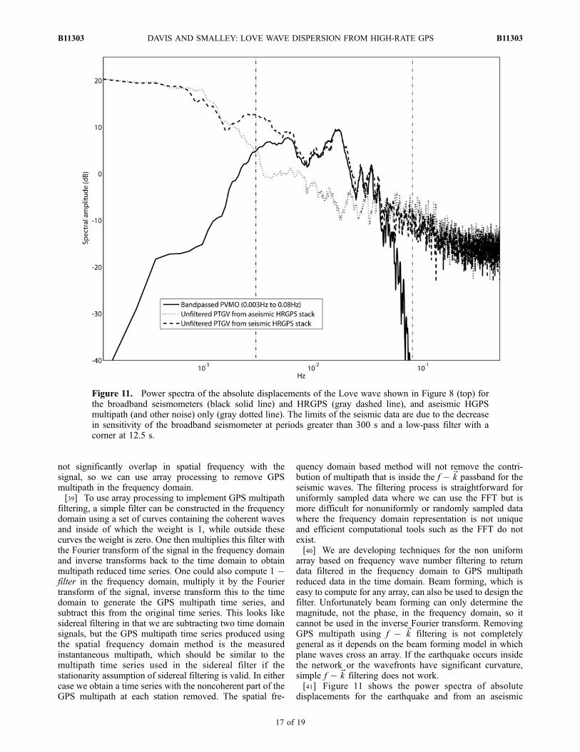
array based on frequency wave number filtering to returndata filtered in the frequency domain to GPS multipathreduced data in the time domain. Beam forming, which iseasy to compute for any array, can also be used to design thefilter. Unfortunately beam forming can only determine themagnitude, not the phase, in the frequency domain, so itcannot be used in the inverse Fourier transform. RemovingGPS multipath using f � ~k filtering is not completelygeneral as it depends on the beam forming model in whichplane waves cross an array. If the earthquake occurs insidethe network or the wavefronts have significant curvature,simple f � ~k filtering does not work.[41] Figure 11 shows the power spectra of absolute

displacements for the earthquake and from an aseismic

Figure 11. Power spectra of the absolute displacements of the Love wave shown in Figure 8 (top) forthe broadband seismometers (black solid line) and HRGPS (gray dashed line), and aseismic HGPSmultipath (and other noise) only (gray dotted line). The limits of the seismic data are due to the decreasein sensitivity of the broadband seismometer at periods greater than 300 s and a low-pass filter with acorner at 12.5 s.


17 of 19

B11303

day, one of the days used to generate the sidereal filter, fromthe colocated HRGPS (PTGV) and broadband (PVMO)stations. The HRGPS time series for PTGV represent theabsolute displacements of the reference site from the ~k = 0beam or spatial filtering stack. As reported by Bilich et al.[2008], but over a narrower frequency band, the HRGPSnoise floor is much higher than that for the broadbandseismometer data, but the two power spectra for the earth-quake data agree well from 0.002 to 0.04 Hz wheresignificant energy is seen in both spectra above their noisefloors. Comparison of the seismic and aseismic powerspectra suggests that the proposal of a dynamic cancellationof GPS multipath during seismic shaking by Bock et al.[2004] is unnecessary. If such a dynamic cancellationoccurred, then GPS multipath would be reduced or removedduring the passage of the seismic waves. Sidereal filteringwould, therefore, be unnecessary during that time, andapplication of sidereal filtering would insert the dynamicallycanceled GPS multipath back into the time series. As withthe case above, where it is not possible to distinguishabsolute from relative displacement HRGPS time serieswhen comparing them to absolute displacement seismicdata, it is not generally possible to see the effects ofmultipath on the seismic time series when the seismic wavesare well above the noise.[42] The Sumatra-Andaman earthquake also generated

large amplitude Rayleigh waves. The N-S azimuth toCNA is close to nodal for Rayleigh waves, however, andthe Rayleigh waves are smaller than the Love waves. Usingbeam forming we were able to detect, but not fully analyze,Rayleigh waves on the radial horizontal component (north-south), but not on the vertical, component. This is notsurprising as GPS is less precise, by a factor of 3–5, inthe vertical.

6. Conclusions

[43] We have shown HRGPS displacement time seriescan be used to produce surface wave dispersion curves thatcompare very well with those produced by broadbandseismometers. We have also used beam steering to showthat the differential displacement time series can be simplymodeled as the difference of the absolute motions of thereference and kinematic stations. Using the relative dis-placements of all the kinematic stations to form the spatialfilter, which is the~k = 0 beam of beam forming, we obtainestimates of the absolute displacement, multipath, and noiseof the reference station plus the GPS common mode noise.When this ~k = 0 beam or spatial filter time series issubtracted from the kinematic time series, we obtain abso-lute displacement time series with the common mode, whichcontains common mode noise plus the reference stationcontribution, removed. Using the ~k = 0 beam allowsestimation of absolute displacement time series whether ornot the reference station is being affected by seismic waves.Array processing also does not require processing of asecond network of stations unaffected by the seismic wavesto estimate the common mode noise. By using all the dataavailable, rather than a handful of distant stations, the arrayprocessing ~k = 0 beam produces a better estimation of thecommon mode filter as uncorrelated noise is reduced by afactor of

ffiffiffiffiNp

, where N is the number of stations. The

absolute time series of the reference station, which alsocontains the common mode noise, can be included in thebeam steer of the absolute displacement time series. Thiswould have a negligible effect on the results of the beamsteer with almost 100 stations, but would allow for bothmultipath and common mode noise removal from thereference station time series by the f � ~k filtering.[44] For large amplitude displacements at long and very

long periods at teleseismic distances, or associated withhigh accelerations in the epicentral region, HRGPS canprovide an important, and due to the large number ofHRGPS stations, dense seismic wavefield sampling thatcomplements traditional seismic data. For the largest signalsproduced by earthquakes, GPS data are also less susceptibleto clipping than broadband seismometers, although asmentioned earlier, the question of preventing temporallyaliased recording in the epicentral region has not yet beenproperly addressed. Other advantages of GPS are that itproduces an estimate of displacement directly and does nothave to be integrated once or twice from velocity oracceleration respectively as with broadband seismometeror accelerometer data and that the response continues tolonger periods than seismometers. Our preliminary analysisindicates application of frequency wave number ( f � ~k)filtering can provide a GPS multipath reduction method thatwill complement sidereal filtering, and we are currentlyworking on implementation of f � k filtering for nonuni-form or random arrays. GPS multipath and common modenoise reduced, absolute displacement seismograms willfacilitate using HRGPS seismograms for a wide range oftraditional seismic applications, especially slip inversionand estimation of strong motion in the region sufferingpermanent coseismic displacements.

[45] Acknowledgments. The seismic data were obtained from theANSS Cooperative New Madrid Seismic Network and the 1 Hz HRGPSdata from the Michigan, N. Carolina, and Ohio state reference networks, theDOT FAA WASS and CORS networks, and the MAEC GAMA network.This work was supported in part by the Mid-America Earthquake Center(MAEC), an Earthquake Engineering Research Center of the NSF, underaward EEC-9701785. We thank T. Herring, an anonymous reviewer, andthe Associate Editor for constructive reviews.

ReferencesKing, R. W., and Y. Bock (2000), Documentation for the GAMIT GPSanalysis software, Dep. of Earth and Planet. Sci., Mass. Inst. of Technol.,Cambridge.

Almendros, J., J. M. Ibanez, G. Alguacil, and E. Del Pezzo (1999), Arrayanalysis using circular-wave-front geometry: An application to locate thenearby seismo-volcanic source, Geophys. J. Int., 136, 159 – 170,doi:10.1046/j.1365-246X.1999.00699.x.

Bilich, A., J. F. Cassidy, K. M. Larson, and G. P. S. Seismology (2008),Application to the 2002 Mw 7.9 Denali Fault earthquake, Bull. Seismol.Soc. Am., 98(2), 593–606, doi:10.1785/0120070096.

Bock, Y., S. A. Gourevitch, C. C. Councelman, R. W. King, and R. I. Abbot(1986), Interferometric analysis of GPS phase observations, Manuscr.Geod., 11, 282–288.

Bock, Y., R. M. Nikolaidis, P. J. de Jonge, and M. Bevis (2000), Instanta-neous geodetic positioning at medium distances with the Global Position-ing System, J. Geophys. Res., 105(B12), 28,223–28,253, doi:10.1029/2000JB900268.

Bock, Y., L. Prawirodirdjo, and T. I. Melbourne (2004), Detection of arbi-trarily large dynamic ground motions with a dense high-rate GPS net-work, Geophys. Res. Lett., 31, L06604, doi:10.1029/2003GL019150.

Brooks, B. A., M. Bevis, R. Smalley Jr., E. Kendrick, R. Manceda,E. Laurıa, R. Maturana, and M. Araujo (2003), Crustal motion in thesouthern Andes (26�–36�S): Do the Andes behave like a microplate?,Geochem. Geophys. Geosyst., 4(10), 1085, doi:10.1029/2003GC000505.


18 of 19

B11303

Brune, J. N., J. E. Nafe, and J. E. Oliver (1960), A simplified method forthe analysis and synthesis of dispersed wave trains, J. Geophys. Res.,65(1), 287–304, doi:10.1029/JZ065i001p00287.

Burg, J. P. (1964), Three-dimensional filtering with an array of seismo-meters, Geophysics, 29, 693–713, doi:10.1190/1.1439406.

Burr, E. J. (1955), Sharpening of observational data in two dimensions,Aust. J. Phys., 8, 30–53.

Capon, R. (1969), High-resolution frequency-wavenumber spectrum analy-sis, Proc. IEEE, 57, 1408–1418, doi:10.1109/PROC.1969.7278.

Capon, R., R. J. Greenfield, and R. J. Kolker (1967), Multidimensionalmaximum-likelihood processing of a large aperture seismic array, Proc.IEEE, 55, 192–211, doi:10.1109/PROC.1967.5439.

Chen, G. (1998), GPS kinematics positioning for the Airborne Laser Alti-metry at Long Valley, California, Ph.D. thesis, 173 pp., Mass. Inst. ofTechnol., Cambridge.

Choi, K., A. Bilich, K. M. Larson, and P. Axelrad (2004), Modified siderealfiltering: Implications for high-rate GPS positioning, Geophys. Res. Lett.,31, L22608, doi:10.1029/2004GL021621.

Dragert, H., K. Wang, and T. S. James (2001), A silent slip event on thedeeper Cascadia subduction interface, Science, 292, 1525 – 1528,doi:10.1126/science.1060152.

Emore, G., J. Haase, K. Choi, K. M. Larson, and A. Yamagiwa (2007),Recovering absolute seismic displacements through combined use of1-Hz GPS and strong motion accelerometers, Bull. Seismol. Soc. Am.,97(2), 357–378, doi:10.1785/0120060153.

Frosch, R. A., and P. E. Green Jr. (1966), The concept of a large apertureseismic array, Proc. R. Soc. London, Ser. A, 290(1422), 368 –384,doi:10.1098/rspa.1966.0056.

Gangi, A. F., and D. Disher (1968), A space-time filter for seismic models,Geophysics, 33, 88–104, doi:10.1190/1.1439923.

Genrich, J. F., and Y. Bock (1992), Rapid resolution of crustal motion atshort ranges with the Global Positioning System, J. Geophys. Res.,97(B3), 3261–3269, doi:10.1029/91JB02997.

Green, P. E., R. A. Frosch, and C. F. Romney (1965), Principles of anexperimental Large Aperture Seismic Array (LASA), Proc. IEEE, 53,1821–1833, doi:10.1109/PROC.1965.4453.

Hatanaka, Y., T. Hiromichi, A. Yoshiaki, Y. Iimura, K. Kobayashi, andH. Morishita (1994), Coseismic crustal displacements from the 1994Hokkaido-Toho-Oki earthquake revealed by a nationwide continuousGPS array in Japan—Results of GPS kinematic analysis, paper pre-sented at Japanese Symposium on GPS, Natl. Comm. for Geod., Sci.Counc. of Jpn., GPS Consortium of Jpn., Tokyo.

Herring, T. A. (2009a), Documentation of the GLOBK software version10.35, Mass. Inst. of Technol., Cambridge.

Herring, T. A. (2009b), TRACK GPS kinematic positioning program,version 1.21, Mass. Inst. of Technol., Cambridge.

Herring, T. A. (2009c), Example of the usage of TRACK, Massachusetts’sInstitute Mass., Inst. of Technol., Cambridge. (Available at http://geoweb.mit.edu/�tah/track_example/)

Holm, S., B. Elgetun, and G. Dahl (1997), Properties of the beampattern ofweight- and layout-optimized sparse arrays, IEEE Trans. Ultrason. Fer-roelectr. Frequation Control, 44, 983–991, doi:10.1109/58.655623.

Hudnut, K. W., et al. (1994), Co-seismic displacements of the 1992 Landersearthquake sequences, Bull. Seismol. Soc. Am., 84, 625–645.

Ji, C., K. M. Larson, Y. Tan, K. W. Hudnut, and K. Choi (2004), Sliphistory of the 2003 San Simeon earthquake constrained by combining1-Hz GPS, strong motion, and teleseismic data, Geophys. Res. Lett., 31,L17608, doi:10.1029/2004GL020448.

Kanasewich, E. R., C. D. Hemmings, and T. Alpaslan (1973), Nth-rootstack nonlinear multichannel filter, Geophysics, 38, 327 – 338,doi:10.1190/1.1440343.

Kennett, B. L. N., E. R. Engdahl, and R. Buland (1995), Constraints onseismic velocities in the Earth from travel times, Geophys. J. Int., 122,108–124, doi:10.1111/j.1365-246X.1995.tb03540.x.

Kobayshi, R., S. Miyazaki, and K. Koketsu (2006), Source processes of the2005 west off Fukuoka Prefecture earthquake and its largest aftershockinferred from strong motion and 1-Hz GPS data, Earth Planets Space, 58,57–62.

Kouba, J. (2003), Measuring seismic waves induced by large earthquakeswith GPS, Stud. Geophys. Geod., 47, 741 – 755, doi:10.1023/A:1026390618355.

Kreemer, C., W. E. Holt, and A. J. Haines (2003), An integrated globalmodel of present-day plate motions and plate boundary deformation,Geophys. J. Int., 154, 8–34, doi:10.1046/j.1365-246X.2003.01917.x.

Kreemer, C., G. Blewitt, W. C. Hammond, and H.-P. Plag (2006), Globaldeformation from the great 2004 Sumatra-Andaman earthquake observedby GPS: Implications for rupture process and global reference frame,Earth Planets Space, 58, 141–148.

Larson, K., P. Bodin, and J. Gomberg (2003), Using 1-Hz GPS data tomeasure deformations caused by the Denali Fault earthquake, Science,300, 1421–1424, doi:10.1126/science.1084531.

Larson, K. M., A. Bilich, and P. Axelrad (2007), Improving the precision ofhigh-rate GPS, J. Geophys. Res., 112, B05422, doi:10.1029/2006JB004367.

Larson, K. M., E. E. Small, E. Gutmann, A. L. Bilich, J. Braun, andV. Zavorotny (2008a), GPS as a soil moisture sensor, Eos Trans. AGU,89(53), Fall Meet. Suppl., Abstract G41D-08.

Larson, K. M., E. E. Small, E. Gutmann, A. Bilich, P. Axelrad, and J. Braun(2008b), Using GPS multipath to measure soil moisture fluctuations:Initial results, GPS Solut., 12(3), 173–177, doi:10.1007/s10291-007-0076-6.

Miyazaki, S., K. M. Larson, K. Choi, K. Hikima, K. Koketsu, P. Bodin,J. Haase, G. Emore, and A. Yamagiwa (2004), Modeling the ruptureprocess of the 2003 September 25 Tokachi-Oki (Hokkaido) earthquakeusing 1-Hz GPS data, Geophys. Res. Lett., 31, L21603, doi:10.1029/2004GL021457.

Nafe, J. E., and J. N. Brune (1960), Observations of phase velocity forRayleigh waves in the period range 100 to 400 seconds, Bull. Seismol.Soc. Am., 50(3), 427–439.

Nikolaidis, R., Y. Bock, P. J. de Jonge, P. Shearer, D. C. Agnew, andM. Van Domselaar (2001), Seismic wave observations with the GlobalPositioning System, J. Geophys. Res., 106, 21,897–21,916, doi:10.1029/2001JB000329.

Ohta, Y., J. Freymueller, S. Hreinsdottir, and H. Suito (2006), A large slowslip event and the depth of the seismogenic zone in the south centralAlaska subduction zone, Earth Planet. Sci. Lett., 247, 108 – 116,doi:10.1016/j.epsl.2006.05.013.

Oliver, J. (1962), A summary of observed seismic surface wave dispersion,Bull. Seismol. Soc. Am., 52(1), 81–86.

Rost, S., and C. Thomas (2002), Array Seismology: Methods and Applica-tions, Rev. Geophys., 40(3), 1008, doi:10.1029/2000RG000100.

Sella, G. F., T. H. Dixon, and A. Mao (2002), REVEL: A model for Recentplate velocities from space geodesy, J. Geophys. Res., 107(B4), 2081,doi:10.1029/2000JB000033.

Takasu, T. (2006), High-rate precise point positioning: Observation ofcrustal deformation by using 1-Hz GPS data, paper presented at GPS/GNSS Symposium 2006, Tokyo Univ. of Mar. Sci. and Technol., Tokyo,15–17 Nov.

vanDam, T., G. Blewitt, and M. B. Heflin (1994a), Atmospheric pressureloading effects on Global Positioning System coordinate determinations,J. Geophys. Res., 99(B12), 23,939–23,950, doi:10.1029/94JB02122.

vanDam, T., G. Mader, and M. Schenewerk (1994b), GPS detects co-seismic and post-seismic surface displacements caused by the Northridgeearthquake, Eos Trans. AGU, 75(16), Spring Meet. Suppl., 103.

Wang, G.-Q., D. M. Boore, G. Tang, and X. Zhou (2007), Comparisons ofground motions from collocated and closely spaced one-sample-per-second Global Positioning System and accelerograph recordings of the2003 M 6.5 San Simeon, California, earthquake in the Parkfield region,Bull. Seismol. Soc. Am., 97(1B), 76–90, doi:10.1785/0120060053.

Wdowinski, S., Y. Bock, J. Zhang, P. Fang, and J. Genrich (1997), SouthernCalifornia permanent GPS geodetic array: Spatial filtering of daily posi-tions for estimating coseismic and postseismic displacements induced bythe 1992 Landers earthquake, J. Geophys. Res., 102, 18,057–18,070,doi:10.1029/97JB01378.

Whiteway, F. E. (1966), The use of arrays for earthquake seismology, Proc.R. Soc. London, Ser. A, 290(1422), 328 – 342, doi:10.1098/rspa.1966.0054.

��J. P. Davis and R. Smalley Jr., Center for Earthquake Research and

Information, University of Memphis, 3876 Central Avenue, Suite 1,Memphis, TN 38152-3050, USA. ([email protected])


19 of 19

B11303

Documents

Love wave dispersion in central North America determined ... pubs... · Love wave dispersion in central North America determined using absolute displacement seismograms from high-rate