Sensors 2011, 11, 10675-10690; doi:10.3390/s111110675

sensors ISSN 1424-8220

www.mdpi.com/journal/sensors

Article

Low-Cost Oil Quality Sensor Based on Changes in Complex Permittivity

Angel Torres Pérez * and Mark Hadfield

Sustainable Design Research Centre, Bournemouth University, Fern Barrow, Talbot Campus,

Poole, Dorset, BH12 5BB, UK; E-Mail: mhadfield@bournemouth.ac.uk

* Author to whom correspondence should be addressed; E-Mail: angeltp@gmail.com;

Tel.: +44-120-2965-560; Fax: +44-120-2965-314.

Received: 10 October 2011; in revised form: 31 October 2011 / Accepted: 4 November 2011 /

Published: 10 November 2011

Abstract: Real time oil quality monitoring techniques help to protect important industry

assets, minimize downtime and reduce maintenance costs. The measurement of a

lubricant’s complex permittivity is an effective indicator of the oil degradation process and

it can be useful in condition based maintenance (CBM) to select the most adequate oil

replacement maintenance schedules. A discussion of the working principles of an oil

quality sensor based on a marginal oscillator to monitor the losses of the dielectric at high

frequencies (>1 MHz) is presented. An electronic design procedure is covered which results

in a low cost, effective and ruggedized sensor implementation suitable for use in harsh

environments.

Keywords: oil quality; impedance spectroscopy; marginal oscillator; dielectric; permittivity;

lubrication oil; on-line monitoring

1. Introduction

Oil quality sensors provide an indication of the condition of oils by measuring different fluid

characteristics such as viscosity, density, optical (light scattering) and electrical properties (permittivity

and conductance).

Viscosity is an important indicator of oil condition because it changes abruptly when there is a

lubricant breakdown. There are several sensing techniques for performing viscosity and density

OPEN ACCESS

Sensors 2011, 11

10676

measurements. However, most common types of commercially available process rheometers rely on

resonators [1-10]. Resonator measurement principles are based on changes in the resonant frequency

and the damping or Q factor. If the mechanical structure of the resonator is brought into contact with a

fluid or solid medium both resonance frequency and damping are changed depending on the viscosity

and the elasticity of the fluid. A recent review of methods for on-line monitoring of viscosity of

lubrication oils is reported by [11].

Light scattering oil quality sensors rely on spectrometric techniques such as infrared, fluorescence

and Raman spectrometry. The most effective indication of oil condition requires a calibration process

using reference oil sample spectra and regression data analysis to isolate the influence of contaminants

within the spectra [12]. Commercial implementations vary from the simplest and lowest cost sensor

which only monitors the light absorbance at a few frequencies [13], whilst the most complex ones

implement high resolution interferometric spectrometers.

An indication of the condition of oil can be extracted from the fluid electrical properties. In the

current market, several types of oil quality sensors are available based on conductivity and permittivity

measurements at one frequency. The conductivity ones are based on potentiostat measurements. The

electrodes can be based on a polymeric bead matrix structure in which the detection principles are

based on changes to the resistance of the polymer that depend on oxidation products and free

water [14], or electrodes made with dissimilar metals where the potential difference between the

sensitive and reference electrodes can be detected (pH probe) [15] or detecting the point when the

lubricant starts to conduct applying an specific voltage waveform to the electrodes and using current to

voltage converters [16,17]. A conductivity sensor for monitoring degradation of automotive engine oil

based on polymers is studied in [18].

The sensors based on permittivity measurements are classified in two types depending on output.

The first ones only monitor changes in the real part of the permittivity and the output of the second

ones is related to the complex permittivity. The ones that monitor the real part of the permittivity

measure changes in the capacitance of the electrodes whilst the sensors that monitor the complex

permittivity provide output related to the capacitance and dielectric losses. The parameter that relates

these two quantities of the complex permittivity is the dissipation factor (D or tan δ) which is the ratio

between the imaginary part and the real part. The real part of the permittivity can be measured using

low cost electrodes [19] and very simple circuits such as bridges [20,21], resonant circuits [22], astable

multivibrators [23].

All measurement techniques for impedance spectroscopy (IS) are suitable to characterise the

dissipation factor for a broad range of frequencies. For frequencies less than 100 KHz, a voltage bridge

feed by a stable oscillator [24] or the use of an autobalancing bridge method [25] is typically used.

A more detailed description of impedance measurement methods is covered in [26]. This research

presents a low cost method to monitor the oil quality by monitoring changes of the complex

permittivity (tan δ) at high frequencies (>1 MHz).

The complex permittivity of lubrication oils changes with use, mainly because of the process of

oxidation and degradation of additives. This process is affected by the presence of contaminants such

as water, soot particles, acid combustion products, glycol, ferrous and non-ferrous metallic particles.

The degradation of most oils imply the generation of molecules that are generally more polar than the

previous ones. The base oil consists of large hydrocarbon molecules that are generally weakly polar, so

Sensors 2011, 11

10677

the presence of most contaminants results in an increase of one or both parts of the oil’s complex

permittivity [27]. Depending on the geometry of the electrodes, the complex permittivity is directly

related to complex impedance. For simple electrode geometries such as parallel plate and cylindrical

electrodes, the relationship between complex permittivity, capacitance and complex impedance vs.

frequency is analytically obtained. Expressions for the capacitance of parallel plate and cylindrical

capacitors are shown in Table 1. Using the concept of complex relative permittivity, Figure 1, the

complex impedance of a capacitor with losses (C*) can be determined using Equation (1): 1· (1)

The complex capacitance depends on the electrodes geometry and it corresponds to the same

expressions shown in Table 1 using the complex permittivity. The final complex impedance expression

is a function of the sensing electrodes geometry, excitation frequency and the condition of the oil

which is related to complex permittivity. For the cylindrical geometry the procedure for the impedance

determination is shown in Figure 2.

Figure 1. Definition of complex relative permittivity [26].

Table 1. Capacitance for different electrode geometries.

C

Capacitance for parallel plates (F)

AElectrode’s area (m2)

DDistance between electrodes (m)

C 2ln

Capacitance for a cylindrical capacitor (F)

Llength of the cylinder (m)

aradius of the inner cylinder (m)

bradius of the outer cylinder (m)

Sensors 2011, 11

10678

Figure 2. Equivalent circuit for cylindrical electrodes

Lubricating oil is a dielectric material with low losses (it is a good electrical insulator as it has low

conductivity). Therefore, the dissipation factor for oil can be considered much lower than unity and

hence, the real part of the complex permittivity is higher than the imaginary part. The complex

impedance expression suggests a simple circuit for the cylindrical electrode system as shown in

Figure 2. This equivalent circuit consists of one capacitor and one resistor connected in series

(equivalent series resistor, ESR). The equivalent circuit helps to understand the influence of the real

and imaginary parts of the complex permittivity in the final impedance expression. The real part of the

permittivity is related to the energy storage and the imaginary part to dielectric losses.

As a result, any measurement of complex impedance of the sensing electrodes is an indicator of the

degradation of the oils. In analytical chemistry the measurement technique of electrode impedance as a

function of frequency is commonly referred to as Electrochemical Impedance Spectroscopy (EIS).

The underlying idea of Impedance Spectroscopy (IS) is the measurement and characterization of a

material-electrode system. A complete impedance spectroscopy analysis involves more than a single

set of measurements of impedance vs. frequency. Frequently, full characterization requires that such

sets of measurements are carried out over a range of temperatures and/or other externally controlled

experimental variables [28].

During the last decade, several research studies considering the application of electrochemical

impedance spectroscopy in lubrication have appeared [29-34]. Important conclusions are drawn

from these studies; the impedance response is dependent on the electrode’s geometry and its contact

with the medium. A diagram of the effects in impedance of temperature, oxidation and water

contamination [29-34] is shown in Figure 3.

It is concluded from the electrochemical studies and patents of impedance measurements of

lubrication oils [29-34] and the Nyquist plots that low frequencies are the most sensitive to variations

in impedance due to changes of the dielectric constant of the fluid. However, the shortcoming of

performing low frequency impedance measurements is that small deviations of the measurement

frequency lead also to great changes in impedance. Yet, high frequency impedance measurements

provide similar readings of impedance at the vicinities of the nominal measurement frequency.

However, high frequency impedance measurements provide lower sensitivity to detect changes in the

dielectric constant of the fluid under test. Finally, this paper discusses the design of a low cost and

effective oil quality circuit capable to monitor changes in the real part of the impedance of the sensing

electrodes at high frequencies.

Sensors 2011, 11

10679

Figure 3. Nyquist diagram showing the influence of temperature and contamination in the

impedance.

2. Sensor Design

2.1. Operation Principles

The range of complex permittivity for different lubricant degradation stages can be obtained using

an impedance analyzer performing impedance frequency sweeps. According to Collister [27], the

values of the dissipation factor (tan δ) are between 0.001 and 0.1 within 1–300 MHz (0.001 for an

unused mineral oil and 0.1 for a heavily contaminated sample) and the real permittivity is typically

2.25 (unused oil) to 2.45 respectively ( ). A frequency sweep example of the dissipation factor

for lubricant at 75 °C without and with water contamination is shown in Figure 4. As it can be seen,

the dissipation factor increases with water contamination. At lower frequencies the increment in

dissipation factor for the oil without and with oil contamination is slightly larger than at higher

frequencies.

Figure 4. tan δ sweep for a lubricant without water contamination and contaminated with water.

Sensors 2011, 11

10680

The working range of impedance, Figure 5, is obtained using the expected range of complex

permittivity and the geometrical dimensions of the sensor’s cylindrical head (Table 2). The real part of

Z (ESR) is within the range of 1 to 1 kΩ within this frequency range. The impedance chart of Figure 5

highlights the real part of Z varies in a larger range (2 decades) than the imaginary part (low range of

values). Any circuit which monitors the real part of the impedance is more sensitive than a circuit

which only measures the imaginary part. Therefore, any method to monitor the degradation of oils

using capacitive measurements (imaginary part of the impedance) is not as effective as methods that

monitor the dielectric losses.

Table 2. Geometrical dimensions of sensor electrodes and expected capacitance.

Cylindrical head

L (mm) b (mm) a (mm) C0 (pF), ε0 C (pF),

(εr = 2.25) C (pF),

(εr = 2.45) 12 8 7 50 112 122

Figure 5. Operational range of impedance for the sensor (cylindrical head).

2.2. Circuit Design

The hardware schematic of the sensing part is shown in Figure 6. The complete sensor comprises a

sensing head which is a cylindrical capacitor made of copper with geometrical dimensions as shown in

Table 2, an LC oscillator circuit implemented with a current feedback amplifier (CFA), an oil

temperature sensor embedded in the sensor’s head (NTC thermistor), some signal conditioning stages

and one microcontroller (MCU). The MCU performs ADC conversions and it implements the

temperature and calibration functions. As an option, the MCU supports industrial communications

protocols such as RS232/RS485 and 4–20 mA.

106

107

108

10-1

100

101

102

103

104

Re

al p

art

of Z

106

107

108

-105

-104

-103

-102

Frequency Hz

Ima

gin

ary

pa

rt o

f Z

Sensors 2011, 11

10681

Figure 6. Hardware schematic (analog part).

2.2.1. Oil Temperature Sensing Circuit

Oil temperature is measured using an NTC thermistor embedded in the sensor head that is

contacting the inner electrode of the cylindrical capacitor (the outer electrode is grounded). The

selected thermistor has a resistance of 20 kΩ at 25 °C and its resistance is adjusted according to the

regression model proposed by Steinhart, Equation (2). 1 (2)

Sensors 2011, 11

10682

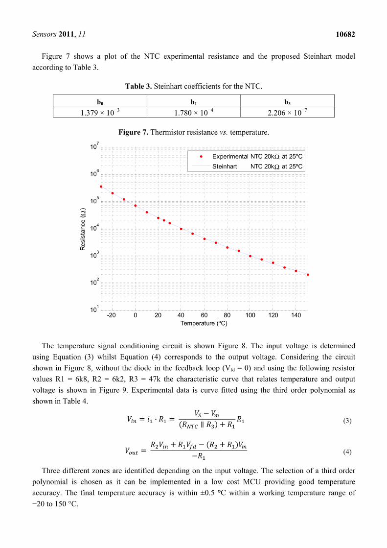
Figure 7 shows a plot of the NTC experimental resistance and the proposed Steinhart model

according to Table 3.

Table 3. Steinhart coefficients for the NTC.

b0 b1 b3

1.379 × 10−3 1.780 × 10−4 2.206 × 10−7

Figure 7. Thermistor resistance vs. temperature.

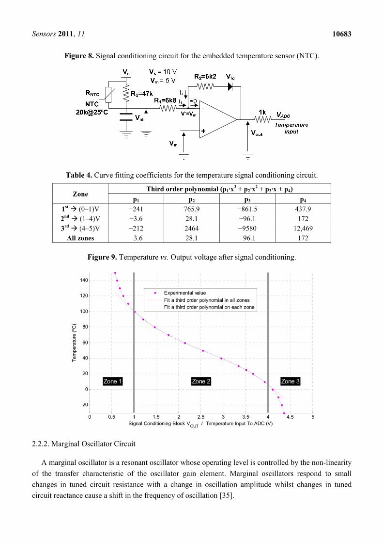
The temperature signal conditioning circuit is shown Figure 8. The input voltage is determined

using Equation (3) whilst Equation (4) corresponds to the output voltage. Considering the circuit

shown in Figure 8, without the diode in the feedback loop (Vfd = 0) and using the following resistor

values R1 = 6k8, R2 = 6k2, R3 = 47k the characteristic curve that relates temperature and output

voltage is shown in Figure 9. Experimental data is curve fitted using the third order polynomial as

shown in Table 4. · (3)

(4)

Three different zones are identified depending on the input voltage. The selection of a third order

polynomial is chosen as it can be implemented in a low cost MCU providing good temperature

accuracy. The final temperature accuracy is within ±0.5 °C within a working temperature range of

−20 to 150 °C.

-20 0 20 40 60 80 100 120 14010

1

102

103

104

105

106

107

Temperature (ºC)

Res

ista

nce

( Ω)

Experimental NTC 20kΩ at 25ºC

Steinhart NTC 20kΩ at 25ºC

Sensors 2011, 11

10683

Figure 8. Signal conditioning circuit for the embedded temperature sensor (NTC).

Table 4. Curve fitting coefficients for the temperature signal conditioning circuit.

Zone Third order polynomial (p1·x

3 + p2·x2 + p3·x + p4)

p1 p2 p3 p4

1st (0–1)V −241 765.9 −861.5 437.9 2nd (1–4)V −3.6 28.1 −96.1 172 3rd (4–5)V −212 2464 −9580 12,469

All zones −3.6 28.1 −96.1 172

Figure 9. Temperature vs. Output voltage after signal conditioning.

2.2.2. Marginal Oscillator Circuit

A marginal oscillator is a resonant oscillator whose operating level is controlled by the non-linearity

of the transfer characteristic of the oscillator gain element. Marginal oscillators respond to small

changes in tuned circuit resistance with a change in oscillation amplitude whilst changes in tuned

circuit reactance cause a shift in the frequency of oscillation [35].

0 0.5 1 1.5 2 2.5 3 3.5 4 4.5 5

-20

0

20

40

60

80

100

120

140

Tem

pera

ture

(ºC

)

Signal Conditioning Block VOUT

/ Temperature Input To ADC (V)

Zone 1 Zone 2 Zone 3

Experimental value

Fit a third order polynomial in all zonesFit a third order polynomial on each zone

Sensors 2011, 11

10684

2.2.2.1. Frequency of Oscillation

The oscillator circuit is shown in Figure 10. The transfer function of the product of amplifier and

feedback circuit is obtained from Figure 10(D). The transfer function of the circuit (Aβ) is shown in

Equation (5). The oscillation condition is obtained using the simplified small signal model,

Figure 10(D). According to Nyquist criterion, the oscillation condition is achieved when the phase of

Aβ is 0 and the gain is greater than 1 at the oscillation frequency ωosc Using the simplified CFA

model [36], the oscillation condition is determined for pure reactive elements, Equation (6). As it can

be seen the oscillation condition is imposed by the inductor and sensing capacitor. Therefore to satisfy

this condition, the term X2 + X3 should be 0 in equation to make Aβ real.

Figure 10. Simplified CFA model to obtain the oscillation condition.

A. Oscillator circuit B. Procedure to obtain Aβ

C. Simplified model for a CFA

D. Small signal circuit to obtain the oscillator transfer function Aβ

Sensors 2011, 11

10685

· · (5)

Considering pure reactive elements, the transfer function is reduced to Equation (6): , ,

·

(6)

Imposing the oscillation condition in Equation (6), the following relationship is obtained, Equation (7): 0° 0 · 1 (7)

The frequency of oscillation when X2 is an inductor and X3 a capacitor is fixed by Equation (8): 12 (8)

2.2.2.2. Criteria for Selecting the Optimum Oscillation Frequency

The sensor can be tuned at any frequency within the 1 to 100 MHz range. However, the optimum

design should be chosen considering the lowest measurement frequency (to gain more sensitivity)

that fulfills the requirement of impedance reading variations due to oscillator frequency drifts (e.g.,

ΔZ < 1%). Frequency drifts are due to changes in the reactive elements as shown in Equation (8).

Therefore, the inductor and the capacitors for the oscillator circuit should have a very low temperature

coefficient. Ceramic chip inductors are suitable for this application as they show very low core losses,

high Q values and relatively high inductance stability over the operating temperature ranges.

The optimum frequency selection can be graphically chosen from the frequency sweeps of the

dissipation factor bearing in mind that tan δ is directly related to the complex impedance, Figure 2. For

example, Figure 4 shows the frequency sweeps of the dissipation factor for hydraulic oil without and

with water contamination respectively. Possible candidates for the best operational frequencies seem to

be around 1 MHz where tan δ has almost the same value within a 1 MHz span and 13 MHz where tan

δ is almost constant for oscillator frequency drifts. The lower frequency is optimum because the tan δ

sensitivity of oil degradation is better than the 13 MHz region. As a result, considering these two

observations the best frequency to perform measurements is around the MHz region.

2.2.2.3. Signal Condition of the Oscillation Peak Amplitude

The amplitude of oscillation is buffered using a unity gain non-inverter CFA. The buffered signal

passes through a peak detection circuit which consists in a diode and one capacitor. This circuit stores

a voltage proportional to the peak of oscillation. A further stage is required to translate the peak

Sensors 2011, 11

10686

amplitude to MCU voltage levels (0 to 5 V). The amplifier inverts the input signal and performs

voltage translation in such way that an increase of output signal corresponds to an increase of ESR or

dissipation factor. The selected stage also compensates the peak detector circuit voltage drop due to the

forward voltage of the diode which is temperature dependant. The governing equation of the whole

peak amplitude detection circuit is plot in Figure 11.

Figure 11. Output voltage proportional to tan δ depending on the peak voltage of the

oscillation waveform.

3. Results and Discussion

The oscillator circuit of Figure 10(A) was simulated using ISIS v7.6 distributed by Labcenter

Electronics. The PSPICE amplifier model used by the simulator is more realistic than the simplified

one used to obtain the frequency of oscillation, therefore obtained results are closer to real circuit

operation. Simulation helps to understand the effect of R1, L2, C1, C3 in the voltage peak of oscillation

and oscillation frequency. The following list of components were used: the CFA is AD8001, R1 is 2 Ω,

R2 is 300 Ω, C1 is 820 pF and C3 is the equivalent load. The following sine wave parameters were

obtained for different equivalent sensor loads, Table 5. The sensitivity of the circuit is not linearly

dependant with the range of ESR. The circuit can detect small changes of ESR with excellent

resolution between 1 to 10 Ω which corresponds to the sensor output voltage within the range 0 to 3 V.

From 10 to 100 Ω the sensitivity is much lower which corresponds to the sensor output voltage within

the range 4 to 4.5 V and finally from 100 Ω onwards the sensors sensitivity is very coarse.

Lubricant samples were prepared under specific oxidation conditions. Air was pump into a vessel

containing lubricant. The temperature of the vessel is controlled using a heating bath with PID

temperature control. Copper wire catalyst is used to accelerate the oxidation process. Five samples at

different oxidation stages were obtained exposing an oil of grade 15W/40 under 150 °C for 0, 8, 16, 24,

32 h. After sample preparation the output of the sensor was recorded for a range of temperatures within

20 °C to 150 °C. Results are shown in Figure 12.

5 5.5 6 6.5 7 7.5 8 8.5 9 9.5 100

0.5

1

1.5

2

2.5

3

3.5

4

4.5

5

Peak voltage of the oscillation waveform, Vin (V)

Vol

tage

out

put

( in

dire

ctly

rel

ated

to

tan δ

), V

out

(V)

ESR / Dissipation factor increases

Sensors 2011, 11

10687

Table 5. Simulation results for the equivalent sensing circuit.

Equivalent load, sensing head Peak of voltage oscillation (V)

ESR (Ω) C (pF)

1 40 (air ε0) 6.1 1 112 >10 (CFA is saturated) 1 116 >10 (CFA is saturated) 1 120 >10 (CFA is saturated)

2.5 120 9.0 5 120 8.1

7.5 120 7.4 10 112 7.1 10 116 7.1 10 120 7.1 25 120 6.1 50 120 5.7 75 120 5.5

100 112 5.4 100 116 5.4 100 120 5.4

Figure 12. Sensor’s output voltage vs. temperature for different oil oxidation stages.

At a given temperature the output voltage is proportional to the oxidation stage. The experimental

data in Figure 12 is curve fitted to different regression models in order to obtain the temperature

dependency of the sensor’s output. As shown in Figure 13, a linear model fits the data (5 datasets) with

a good degree of accuracy (m = −0.01123, b = 2.422). The selected model can be implemented in a

MCU to compensate temperature drifts due to temperature variations.

20 40 60 80 100 120 140 0

0.2

0.4

0.6

0.8

1

1.2

1.4

1.6

1.8

2

2.2

2.4

2.6

2.8

3

Temperature (ºC)

Vo

ltag

e o

up

ut (

V)

oil A (0h)oil B (8h)oil C (16h)oil D (24h)oil E (32h)

Sensors 2011, 11

10688

Figure 13. Regression models to extract the temperature dependency. (All samples were

considered, Oil A,B,C,D,E)

The same procedure for temperature compensation can be applied to a specific machine lubricant.

The experimental dataset consists on lubricant samples at different degradation stages and sampling

time intervals. As a result, a custom based calibration approach could be performed providing a more

meaningful indication of the oil condition for a specific industry asset.

4. Conclusions

Impedance monitoring of lubricants is an important tool for detecting the condition of oils. A low

cost oil quality sensor based on a marginal oscillator is presented which monitors changes on the

impedance of the sensing electrodes at high frequencies. The circuit provides a voltage output related

to the dissipation factor and therefore, it provides an indication of the oil condition as the dissipation

factor tends to increase with the increasing presence of contaminants in lubrication oil. The proposed

sensor shows three important features: it is a very low cost design, it can be custom calibrated for a

specific lubricant and it provides effective oil quality detection. This conclusion means that this sensor

is an attractive alternative compared with other types of oil condition sensors.

Acknowledgments

The authors acknowledge the financial support of the EPRSC and RNLI.

References

1. Roth, W.; Rich, S.R. A new method for continuous viscosity measurement: General theory of the ultra‐viscoson. J. Appl. Phy. 1953, 7, 940-950.

20 40 60 80 100 120 140 0

0.2

0.4

0.6

0.8

1

1.2

1.4

1.6

1.8

2

2.2

2.4

2.6

2.8

3

Temperature (ºC)

Vo

ltag

e o

up

ut (

V)

oil A (0h)oil E (32h)linear modelquadratic modelcubic model

Sensors 2011, 11

10689

2. Roth, W.; Rich, S.R. Method and apparatus for measuring viscosity of fluid like materials. U.S.

Patent 2,839,915, May 1958.

3. Roth, W.; Rich, S.R. Temperature compensated viscometer. U.S. Patent 2,837,913, May 1958.

4. Loiselle, K.T.; Grimes, C.A. Viscosity measurements of viscous liquids using magnetoelastic

thick-film sensors. Sci. Instrum. 2000, 71, 1441-1446.

5. Jain, M.K.; Grimes, C.A. Effect of surface roughness on liquid property measurements using

mechanically oscillating sensors. Sens. Actuat. A 2010, 100, 63-69.

6. Farone, W.A.; Sacher, R.F.; Fleck, C. Acoustic viscometer and method of determining kinematic

viscosity and intrinsic viscosity by propagation of shear waves. U.S. Patent 6,439,034, August

2002.

7. Leonid Matsiev, J.B.; Mcfarland, E. Method and apparatus for characterizing materials by using

mechanical resonator. U.S. Patent 2004/0074302A1, April 2004.

8. Dual, J.; Sayir, M.; Goodbread, J. Viscometer. U.S. Patent 4,920,787, May 1990.

9. Agoston, A.; Ötsch, C.; Jakoby, B. Viscosity sensors for engine oil condition monitoring

application and interpretation of results. Sens. Actuat. A 2005, 121, 327-332.

10. Markova, L.V.; Myshkin, N.K.; Kong, H.; Han, H.G. On-line acoustic viscometry in oil condition

monitoring. Tribol. Int. 2011, 44, 963-970.

11. Markova, L.V.; Makarenko, V.M.; Semenyuk, M.S.; Zozulya, A.P. Online monitoring of

viscosity of lubrication oils. J. Frict. Wear 2010, 6, 433-442.

12. Meijer, G. Smart Sensor Systems; John Wiley & Sons: West Sussex, UK, 2008; pp. 129-130.

13. Agoston, A. Otsch, C. Zhuravleva, J. Jakoby, B. An IR-absorption sensor system for the

determination of engine oil deterioration. Sensors 2004, 1, 463-466.

14. Voelker, P.J.; Hedges, J.D. Oil quality sensor for use in a motor. U.S. Patent 5,789,665, August

1998.

15. Kuroyanagi, S.; Fujii, T.; Okada, K.; Nozawa, M.; Yamagucho, S.; Naito, K. Oil deterioration

detector. U.S. Patent 5,523,692, April 1996.

16. Schoes, J.N. Oil quality sensor system, method and apparatus. U.S. Patent 6718819B2, April

2004.

17. Wang, S.C.S.; Lee, H.S.; Mcgrath, P.B.; Staley, D.R. Oil sensor systems and methods of

qualitatively determining oil type and condition. U.S. Patent 5,274,335, December 1993.

18. Latif, U.; Dickert, F.L. Conductometric sensors for monitoring degradation of automotive engine

oil. Sensors 2010, 11, 8611-8625.

19. Raadnui, S.; Kleesuwa, S. Low-cost condition monitoring sensor for used oil analysis. Wear 2005,

259, 1502-1506.

20. Hopkins, E.L.; Irwin, K. Instrument for capacitively testing the condition of the lubricating oil.

U.S. Patent 3,182,255, April 1965.

21. Hopkins, E.L.; Wedel, J.L. Fluid condition monitoring system. U.S. Patent 4,064,455, November

1977.

22. Appleby, M.P. Wear Debris Detection and Oil Analysis Using Ultrasonic and Capacitance

Measurements. M.S. Thesis, University of Akron, Akron, OH, USA, 2010.

23. Liu, Y.; Liu, Z.; Xie, Y.; Yao, Z. Research on an on-line wear condition monitoring system for

marine diesel engine. Tribol. Int. 2000, 33, 829-835.

Sensors 2011, 11

10690

24. Allen, K.J.K. Design and Fabrication of a Laboratory Test Unit to Demonstrate the

Characterization and Collection of Data from Condition Monitoring Sensors; Contract Report

No. CR 2005-243; Defence R&D Canada-Atlantic: Dartmouth, NS, Canada, 2004.

25. Lin, Y.; Wang, S.; Resendiz, H. Liquid Properties Sensor Circuit. U.S. Patent 7659731B2,

February 2010.

26. Okada, K.; Sekino, T. Impedance Measurement Handbook; Agilent Technologies: Santa Clara,

CA, USA. Available online: http://cp.literature.agilent.com/litweb/pdf/5950-3000.pdf (accessed

on 31 October 2011).

27. Collister, C.J. Electrical measurement of oil quality. U.S. Patent 6,459,995, October 2002.

28. Macdonald, J.R. Impedance Spectroscopy. Ann. Biomed. Eng. 1992, 20, 289-305.

29. Ulrich, C.; Petersson, H.; Sundgren, H.; Björefors, F.; Krantz-Rülcker, C. Simultaneous

estimation of soot and diesel contamination in engine oil using electrochemical impedance

spectroscopy. Sens. Actuat. B 2007, 127, 613-618

30. Boyle, F.P.; Lvovich, V.F. Method for on-line monitoring of condition of non-aqueous fluids.

U.S. Patent 7,355,415, April 2008.

31. Smiechowski, M.F.; Lvovich, V.F. Characterization of non-aqueous dispersions of carbon black

nanoparticles by electrochemical impedance spectroscopy. J. Electroanal. Chem. 2005, 577, 67-78.

32. Lvovich, V.F.; Skursha, D.B.; Boyle, F.P. Method for on-line monitoring of quality and condition

of non-aqueous fluids. U.S. Patent 6861851B2, March 2005.

33. Lvovich, V.F.; Smiechowski, M.F. Impedance characterization of industrial lubricants.

Electrochim. Acta 2006, 51, 1487-1496.

34. Lvovich, V.F.; Smiechowski, M.F. Non-linear impedance analysis of industrial lubricants,

Electrochim. Acta 2008, 53, 7375-7385.

35. Idoine, J.D.; Brandenberger, J.R. FET marginal oscillator circuit. Rev. Sci. Instrum. 1971, 42,

715-717.

36. Current Feedback Amplifier Theory and Applications; Application Note AN9420; Intersil: Austin,

TX, USA, 1995.

© 2011 by the authors; licensee MDPI, Basel, Switzerland. This article is an open access article

distributed under the terms and conditions of the Creative Commons Attribution license

(http://creativecommons.org/licenses/by/3.0/).