Embed Size (px)
Citation preview
CAROLINA CORREIA GONÇALVES DENTE
LOW-FIELD MRI IN HORSES DIAGNOSED WITH
PALMAR FOOT PAIN
Coordinator: Prof. Doutor Manuel Pequito
Co-Coordinator: Dr. Med. Vet. Klaus-Peter Neuberg
LUSOFONA UNIVERSITY OF HUMANITIES AND TECHNOLOGIES
VETERINARY MEDICINE FACULTY
LISBON
2018
1
CAROLINA CORREIA GONÇALVES DENTE
LOW-FIELD MRI IN HORSES DIAGNOSED WITH
PALMAR FOOT PAIN
LUSOFONA UNIVERSITY OF HUMANITIES AND TECHNOLOGIES
VETERINARY MEDICINE FACULTY
LISBON
2018
Dissertation submitted to achieve the Master Degree in Veterinary
Medicine in the Integrated Course of Veterinary Medicine given by Lusófona
University of Humanities and Technologies (FMV-ULHT) on 16th of April,
2018. With the Rectory Dispatch number 118/2018 and with the following
constitution of the jury:
PRESIDENT: Profª Doutora Laurentina Pedroso
ARGUING: Prof. Doutor Mário Cotovio
COORDINATOR: Prof. Doutor Mário Pequito
VOWEL: Profª Doutora Sofia van Harten

2
It is only with the heart that one can see rightly. What is essential is
invisible to the eye.
Antoine de Saint-Exupery

3
To my mother, my father, my siblings
To my two stars in the sky
To those who supported me incondicionally
4
Acknowledgments
This dissertation is the result of a journey that started in the University of Lusófona, and
for that reason, I would like to start thanking to the city and to the University that gave me the
best moments of my live.
To all my teatchers and colleges that I met during the last 6 years but speacially to my
friends Sofia, Mariana, Pipa, Joana and Inês, for being part of my journey, for the crazy nights
before every exam, for the nights out and, the afternoons in the university bar, for supporting
me and being true friends.
To Ricardo, Margarida, Marta e Alexandre for introducing me to my university, the tips
for the exams and being part of my academic course.
To Professor Manuel Pequito, for the support and guidance given to do this work and
for being always available when I needed.
To Professora Inês Viegas, for all the support and help with the statistics. I am sure that
this work would be much harder without her help.
To all the team of Pferdeklinik Leichlingen, for taking me in and provinding me with
the best externship I could ever wished for. A special thank to my friends Alina, Greta, Larissa,
Rosa, Tarek and Vivien for all the support and good advices through the hard times, specially
when I was missing home so much.
To Dr. Nolting, Dr. Krebs and Dr.von Plato for giving me the opportunity to stay.
To Birte and Joost for teaching me everything I know about MRI, and for all the
pacience through the process.
To Carla Bom and Go4Word, for all the help and support. But also for being a friend of
the family.
To KP. I will never be able to repay everything and I can just hope, that one day, I will
be able to do for someone the same you did for me. The best teacher I could ever ask for, a
friend and someone to look up to, someone that cheered me up when I was felling down,
someone that supported me and believed in me uncondicionally. Thank you for everything and
for making the last 2 years the best experience in my life.

5
To my best friend Débora Oliveira e Miguel Durão just because they are the best friends
in the world. For everything we went through together and for being always there no matter the
distance.
To my uncle Tó Dente, for all the pressure, support and help to finish this work and for
everything else in the last 6 years.
To my two grandmothers, because I love you. And for my two guardian angels, because
I know that up there, they look up for me every single day.
To my family. My mother, my father and my siblings, Clara and Guilherme. The ones
that I love the most and for being so precious to me. To my father and my mother for all the
incondicional love and support everyday in my life, for believing in me, for being always there
no matter what, for making this dream come true and for being the best parents in the world.
To Clara and Guilherme for every joy, for the support and love, for being the best siblings and
for making me so proud of their everyday accomplishments.
To Tita, Chloe, Kiko and Maggy for making me realise that I wanted to be a veterinarian.
For all the love and for being my inspiration every single day.

6
Resumo
É reconhecido, hoje em dia, que o que até então era agrupado na vaga categoria
diagnóstica de síndrome podotroclear, pode ser o resultado de diferentes patologias em
diferentes tecidos no casco, que poderão ocorrer concomitantemente. O desenvolvimento de
técnicas imagiológicas mais sensíveis poderá proporcionar um melhor conhecimento acerca das
causas de dor proveniente da região do casco.
Visto que as imagens de ressonância magnética se baseam nas propriedades magnéticas
de protões, não são utilizadas radiações ionizantes como acontece em outras técnicas
imagiológicas. Ã grande vantagem em comparação às outras modalidades imagiológicas é o
potencial de deteção de lesões em tecidos moles, bem como lesões ao nível do osso e cartilagem.
O principal objectivo deste estudo foi avaliar a prevalência de lesões encontradas no
casco, em cavalos de desporto com claudicação crónica em membros anteriores e submetidos
a um exame de ressonância magnética. Secundariamente, foi avaliada a tendência para
ocorrência das lesões encontradas, uni- ou bilateralmente. Ainda, das lesões encontradas, foi
estudada a ocorrência de lesões em associação.
Neste estudo foram utilizados 95 cavalos de desporto de diferentes disciplinas. Lesões
no osso navicular foram as mais frequentes (38%), seguido de lesões na articulação
interfalângica distal (16%) e no tendão flexor digital profundo (15%). Diferentes combinações
de lesões foram encontradas entre diferentes tecidos. Lesões no osso navicular apareceram de
forma difusa (18%), com lesões que afetaram o bordo distal, superfície dorsal e flexora (12%),
com lesões que afetaram o bordo distal e superfície flexora (9%) e com lesões que afetaram a
superfície flexora e dorsal (1%). Na amostra estudada, não ocorreram lesões isoladas no bordo
proximal e na superfície dorsal do osso navicular.
A Ressonância Magnética é uma excelente ferramenta de diagnóstico de problemas de
casco quando comparada com as outras técnicas disponíveis. Devido aos elevados custos do
exame, não deverá ser utilizada rotineiramente e só após um exame de claudicação rigoroso e
quando não é possível chegar a um diagnóstico definitivo através de outras técnicas
imagiológicas.
Palavras-chave: Ressonância magnética, cavalos, síndrome podotroclear, técnicas
imagiológicas, osso navicular.

7
Abstract
It is well recognised today, that the underlying pathology for the so called “palmar foot
pain” or “navicular syndrome” can be a result of either single or multiple pathologies in
different tissues in the hoof. The development of advanced diagnostic imaging modalities such
as MRI, have taken the understanding of these conditions to a different level.
Since MRI is based on magnetic properties of protons, it uses no ionizing radiation
unlike other imaging techniques, such as radiology and CT. The main advantage of MRI in
comparison to the other tecnhiques is its ability to highlight soft tissue lesions, as well as
cartilage and bone.
The main objective of this study was to evaluate the prevalence of lesions in a population
of sport horses presented with a chronic forelimb lameness that underwent an MRI examination.
Also, was evaluated uni- or bilateral tendency of occurrence, of the lesions found and see if
they accurred in association.
This study contemplated 95 sport horses from different disciplines. Navicular bone
lesions were the most frequent (38%), followed by coffin-joint (16%) and DDFT (15%) lesions.
Several of different combinations of lesions were seen among all the tissues. Lesions in the
navicular bone appeared as a diffuse disease (18%), had lesions affecting the distal border,
dorsal and flexor surface (12%), had lesions affecting the distal border and flexor surface (9%)
and lesions affecting the flexor and dorsal surface (1%). Lesions of the proximal border and
dorsal surface of the navicular bone did not occur without association to other areas of the
navicular bone, in the population.
MRI proved to be an excellent tool to diagnose pathologies within the foot when
compared to the other imaging techniques available. An accurate clinical lameness examination
to include diagnostic analgesia is still crucial to confirm the localization to be within the foot.
Due to the high cost of MRI, it should only be considered if other and less cost imaging
tecnhiques fail to provide an accurate diagnosis.
Key words: MRI, horses, palmar foot pain, navicular syndrome, diagnostic imaging modalities,
navicular bone.

8
Resumo das secções em Português
Introdução à Ressonância Magnética
A ressonância magnética é uma técnica de diagnóstico de imagem que depende da
distribuição e concentração de iões de hidrogénio nos tecidos biológicos, das suas propriedades
e como cada um reage à presença de um campo magnético (Labruyère & Schwarz, 2013;
Lauterbur, 1973). Os iões de hidrogénio são um dos mais sensíveis aos gradientes de campo e
a sua elevada abundância nos tecidos biológicos tornam possível a criação de imagens sem a
necessidade de adição e/ou exposição a outras substâncias (Armstrong & Stephen, 1991).
Apesar de o sinal de ressonância magnética poder ser detetado em vários tipos de iões, são
utilizados iões hidrogénio devido aos benefícios já mencionados (Armstrong & Stephen, 1991;
Murray, 2011).
A ressonância magnética cria imagens através da deteção de sinal dos iões de
hidrogénio presentes na água e gordura dos tecidos biológicos (Armstrong & Stephen, 1991;
Damadian, 1971; Lauterbur, 1973). A parte do corpo a ser examinada deverá, para isso, ser
colocada sob influência de um campo magnético e sujeita a pulsos de radiofrequências. Os iões
de hidrogénio irão ganhar energia e vão emitir um sinal de radiofrequência em retorno que é
recolhido e utilizado para a formação da imagem (Armstrong & Stephen, 1991; Labruyère &
Schwarz, 2013). A intensidade do sinal varia de tecido para tecido devido às diferenças de
concentração e distribuição de iões de hidrogénio e ao estado dos mesmo, i.e. quimicamente
livres ou ligados. Estas diferenças resultam em aparências diferentes dos tecidos na mesma
imagem (Armstrong, 1991).
O casco a examinar é colocado num campo magnético e é posteriormente aplicada
uma bobina de transmissão e deteção de sinal. Os pulsos de radiofrequência são transmitidos
ao paciente pela bobina, absorvidos pelos iões de hidrogénio, que por sua vez ganham energia,
e retransmitem um sinal de radiofrequência, que é recolhido pela mesma bobina (Armstrong &
Stephen, 1991). O sinal de radiofrequência emitido pelos iões de hidrogénio vai depender da
densidade de protões, i.e. do número de iões de hidrogénio presentes em cada tecido, e dos
tempos de relaxamento T1 e T2 (Armstrong & Stephen, 1991; Murray, 2001).

9
Os tempos de relaxamento T1 e T2 refletem a taxa com que os iões de hidrogénio
perdem a energia (Armstrong & Stephen, 1991). Todas as imagens de ressonância magnética
contêm informação de ambos os tempos de relaxamento, contudo, através da manipulação dos
parâmetros do sistema, a imagem poderá ser maioritariamente dependente de um ou de outro
(Armstrong & Stephen, 1991). Várias combinações de pulsos e campos magnéticos podem ser
usados para criar imagens com diferentes contrastes (Labruyère & Schwarz, 2013).
Quando o paciente é colocado sob influência do campo magnético, os núcleos dos iões
de hidrogénio vão alinhar-se com a direção do mesmo (Armstrong & Stephen, 1991; Murray,
2011). Pulsos de radiofrequência que são emitidos pela bobina fazem com que algum dos
núcleos fiquem desalinhados relativamente à direção do campo magnético. Quando a bobina é
desligada e cessa a emissão de pulsos, os protões tendem a regressar ao equilíbrio original, i.e.
ao alinhamento com a direção do campo magnético.Este fenómeno é acompanhado por uma
libertação de energia sob a forma de sinal de radiofrequência, que será captado novamente pela
bobina (Labruyère & Schwarz, 2013).
O tempo de relaxamento T1 representa a velocidade em que os protões excitados
realinham com a direção do campo magnético.
O tempo de relaxamento T2 reflete a taxa de declínio do sinal devido ao desfasamento
dos protões no seu “spin” (Armstrong & Stephen, 1991).
As imagens são produzidas dentro de uma escala de tons cinza com vários tipos de
contraste, sendo o resultado da intensidade do sinal (Mair et al., 2005). A aparência do tecido
na imagem é afetada pela sua natureza, pelo sistema, sequência de pulsos e pelos parâmetros
de aquisição (Armstrong & Stephen, 1991; Labruyère & Schwarz, 2013). Quando existe uma
lesão num tecido, alterações na sua estrutura, composição bioquímica e distribuição de água
resultam em alterações na aparência da imagem de ressonância magnética (Murray, 2001).
O sinal provém maioritariamente dos iões de hidrogénio móveis presentes na gordura
e água dos tecidos (Armstrong & Stephen, 1991) e por essa razão, estruturas com pouca
quantidade de hidrogénio ou poucos iões móveis terão aparência negra (Mair et al., 2005;
Murray, 2001).
O contraste é determinado pela quantidade de iões de hidrogénio , tempos de
relaxamento T1 e T2 (Armstrong & Stephen, 1991) e pela manipulação da sequência de pulsos.

10
Por esta razão, o mesmo tecido terá aparências diferentes em imagens T1, T2 e PD (Labruyère
& Schwarz, 2013; Murray, 2001).
Imagens referidas como T1 ou T1W o contraste depende do tempo de relaxamento T1,
imagens referidas como T2 ou T2W o contraste depende do tempo de relaxamento T2 e imagens
referidas como PD ou PDW o contraste depende do número de protões de hidrogénio livre ou
móvel (Murray, 2011).
O tempo de relaxamento T1 é longo para fluídos, mas muito curto para tecidos
baseados em gordura. Em imagens T1W tecidos ricos em água irão ter uma aparência cinzenta
clara, dependendo da sua quantidade do tecido. Neste caso, o aumento da quantidade de água
irá tornar a imagem mais escura. Tecidos com um aumento do seu conteúdo de água devido a
edema ou aumento da permeabilidade capilar, irão aparecer mais escuros rodeados por uma
zona de tecido de “aparência normal”. Tecidos com composição elevada de gordura irão ter
uma aparência mais clara (Murray, 2011). Imagens T1W providenciam o melhor detalhe
anatómico e por isso são consideradas sequência “standart” para linha de base, num exame
imagiológico (Mair et al., 2005).
Em imagens T2W, a água aparece a branco enquanto que tecidos baseados em água
ou gordura terão sinal intermédio. Imagens T2W têm menos detalhe anatómico e menos
resolução que T1W, mas são extremamente úteis para deteção de patologias onde existe um
aumento da composição de água nos tecidos, tais como edema e inflamação. Neste casos, estas
lesões irão aparecer como áreas com o aumento de intensidade de sinal, i.e. mais claras,
rodeadas por tecido normal e mais escuro. Imagens T2W também são úteis para avaliação de
estruturas sinoviais (Mair et al, 2005; Murray, 2001).
O aumento de conteúdo de água em tecidos ricos em gordura, por uma lesão, tal como
a medula óssea, pode ser difícil de avaliar usando imagens T2W, devido ao sinal proveniente
da gordura. Nestes casos, é usado uma sequência chamada STIR, em que o sinal da gordura é
suprimido, sendo então possível a deteção do sinal de fluídos (Kleiter et al., 1999; Murray,
2011).
A qualidade da imagem em ressonância magnética é determinada pelo sinal, barulho,
contraste e artefactos. O barulho é gerado pelo movimento térmico de eletrões e medidas
deverão ser tomadas para prevenir quaisquer fontes de barulho provenientes do exterior, que
possam ajudar a degradar a qualidade da imagem. Isto pode ser conseguido durante a instalação
11
da sala de ressonância magnética, blindando as paredes, teto, chão e portas com cobre
impedindo ondas de radiofrequência provenientes do exterior. Devem ainda ser aplicadas
proteções especiais em todos os equipamentos eletrónicos dentro da sala de ressonância
magnética (Murray, 2011).
São chamados de artefactos todas as características numa imagem que não representem
a realidade, e que podem levar a mal interpretações ou a diagnósticos incorretos. Ocorrem
frequentemente e podem ser resultado de fatores relacionados com o paciente, com a natureza
da ressonância magnética, técnica de aquisição das imagens e imperfeições do sistema. São
classificados em artefactos de movimento, artefactos de campo magnético heterogéneo e
artefactos digitais (Murray, 2011).
Artefactos de movimento, tal como o nome indica são causados pelo movimento
involuntário ou voluntário durante a aquisição da imagem. São exemplos o movimento pulsátil
de vasos sanguíneos, a respiração ou mesmo pequenos movimentos em cavalos que tenham
recebido demasiada sedação. O resultado será uma imagem com manchas, borrões e
arrastamento de estruturas que poderá levar a uma imagem sem poder diagnóstico. Artefactos
de movimento podem ser minimizados pelo uso de scans MI, uma vez que eles permitem a
aquisição da imagem pelo sistema apenas quando existem movimentos mínimos e por reposição
das fatias quando movimento é detetado. Outas opção será encurtar o tempo de aquisição,
através do uso de scans rápidos ou super-rápidos (Murray, 2001).
Artefactos de campo magnético heterogéneo são causados habitualmente por
flutuações de temperatura ou objetos de metal. Artefactos causados por metal são observados
como áreas sem sinal rodeados por uma halo fino híper-intenso e com distorção das estruturas
adjacentes. A temperatura e humidade deverão ser controladas dentro da sala de ressonância
magnética, para minimizar a ocorrência destes artefactos, e a remoção de peças de metal na área
de segurança do campo magnético. Botas de biqueira de aço deverão ser evitadas, ferraduras
deverão ser removidas e o casco inspecionado para verificar a completa remoção dos pregos de
casco.
Artefactos digitais comtemplam: artefacto de desvio químico, ângulo mágico, e
volume parcial. O desvio químico manifesta-se quando o sinal da água e da gordura se cancelam
mutuamente. Por exemplo em áreas com o aumento de sinal em imagens T2 FSE, que aparecem
mais escuras em T2 GRE. A presença real de fluído pode ser então avaliada usando imagens
STIR. O ângulo mágico manifesta-se por um aumento de sinal em estruturas ricas em fibras de

12
colagénio que se encontram com uma orientação aproximada de 55º graus em relação ao campo
magnético. Imagens T1W e PDW são mais suscetíveis á ocorrência deste artefacto. Estruturas
comummente afetadas incluem os ligamentos colaterais da articulação interfalângica distal,
ligamentos sesamóideos oblíquos, flexor digital profundo e ligamento anular distal. Deve dar-
se preferência ao uso de scans em que este artefacto não ocorra, tais como T2W ou STIR, na
avaliação destas estruturas (Murray, 2001). O artefacto de volume parcial ocorre em
habitualmente em estruturas curvas ou irregulares, onde os limites de uma estrutura aparecem
na mesma fatia em aposição ou parcialmente cruzadas. Este artefacto pode ser evitando
diminuindo a espessura das fatias, através do uso de imagens de alta resolução (Murray, 2001).
Claudicação, Exame Físico e Técnicas Diagnósticas
O exame deverá começar pela recolha dos dados da anamnese e história clínica,
recolhendo informações essenciais como a idade, sexo, raça e uso do cavalo (Hinchcliff et al.,
2004). Perguntas mais detalhadas acerca da história clínica do paciente são essenciais aquando
a tentativa de descobrir a causa da claudicação ou falta de performance. Esta deverão incluir: a
duração do problema, se melhora ou piora com exercício e se sim com quais, como se tem feito
o maneio do problema até á data, história de problemas ortopédicos anteriores, alterações no
maneio ou ferração, entre outros (Ross & Dyson, 2003).
Deverá ser seguido o exame físico do cavalo, começando por observar o cavalo á
distancia, passando á palpação do pescoço, membros anteriores, tórax e coluna e por último os
membros posteriores. Nesta fase deverão ser notadas alterações como inchaços e quaisquer
assimetrias ou presença de dor á palpação.
De seguida é efectuado o exame dinâmico, observado o cavalo em andamento e em
trote em linha recta e em círculo. Nesta fase a claudicação deverá ser identificada bem como os
membros afectados.
Testes de flexão são efetuados na tentativa de exacerbar a claudicação, comparando
sempre com o membro contra lateral. Após o exame físico e identificada a claudicação seguem-
se os bloqueios anestésicos na tentativa de localizar a área do membro de onde provém a dor
(Auer & Stick, 1999; Ross & Dyson, 2003).
13
Antes de efetuar qualquer bloqueio anestésico, deverá ser aplicada uma pinça de casco
e verificar a existência de reação. Os bloqueios deverão ser aplicados da zona distal em direção
proximal do membro (Moyer, 2010). Cavalos com síndrome navicular na grande maioria
melhoram o grau de claudicação com bloqueio digital palmar ainda que muitas vezes a
claudicação só consegue ser completamente eliminada com o bloqueio sesamóideo abaxial
(Ross & Dyson, 2003). Muitos casos podem ainda responder a bloqueios intra-articulares da
articulação interfalângica distal (Moyer, 2010).
Após localização do casco como fonte de claudicação, através do exame físico e
bloqueios anestésicos, exames diagnóstico de imagem deverão ser efetuados. As ferraduras
deverão ser removidas, os cascos limpos e um conjunto de radiografias deverão ser tiradas que
incluem projeções lateromedial e dorsopalmar do casco em estação sobre um bloco, projeções
dorsoproximal-palmarodistal e palmaroproximal-palmarodistal.
Infelizmente, o exame radiográfico permite apenas a visualização de alterações ao
nível dos ossos e articulações (Rijkenhuisen, 2006; Kristoffersen & Thoefner, 2003; Butler et
al., 2000) e os bloqueios anestésicos ajudam apenas no isolamento da área de interesse não
indicando a distribuição nem a severidade do problema (Kristoffersen & Thoefner, 2003).
Ecografia é uma técnica de diagnóstico complementar á radiografia, usado
rotineiramente na avaliação de tecidos moles (Busoni & J.-M. Denoix, 2001). O exame
ecográfico ao aparelho podotroclear inclui duas abordagens: suprasesamoidana, realizada na
parte distal da quartela e infrasesamoidana, através da sola do casco (Jacquet & J.-M. Denoix,
2012; Busoni & Jean-Marie Denoix, 2001). Ambas as técnicas têm as suas limitações: na
abordagem suprasesamoidana, apenas a parte proximal do aparelho podotroclear é avaliado
(Busoni & Jean-Marie Denoix, 2001) enquanto que na abordagem infrasesamoidana está
limitada á conformação da ranilha do casco, em que se os sulcos forem muitos profundos
impendem o acoplamento entre a sonda e a superfície da ranilha (Jacquet & J.-M. Denoix,
2012).
Na abordagem infrasesamoidana a preparação do casco e da ranilha é essencial para
obtenção de imagens de qualidade. A ranilha deverá ser lavada com água quente e sabão e
aparada com a ajuda de uma faca de cascos (Kristoffersen & Thoefner, 2003). Posteriormente
deve ser aplicado um penso molhado de casco durante pelo menos 15 minutos para ajudar a
suavizar a superfície da ranilha (Busoni & J.-M. Denoix, 2001). Em casos de falha de
14
diagnóstico após a realização de exames radiográficos e ecográficos, exame de ressonância
magnética deverá ser visto como opção.
A ressonância magnética é a modalidade imagiológica com mais sensibilidade na
deteção de lesões e não só é considerada uma excelente ferramenta por conseguir ultrapassar
limitações de outras técnicas imagiológicas em avaliar as estruturas do casco, mas também
porque ajuda a redirecionar o tratamento e reabilitação e a fornecer prognóstico (Murray, 2011;
Barret et al., 2016 & Mair et al., 2005). Ajuda ainda na deteção de lesões subtis que
normalmente não são detetáveis por outras técnicas imagiológicas e por essa razão é
considerada técnica “standard” na deteção de lesões ao nível do casco. Também poderá ajudar
a determinar se um caso é candidato para neurectomia digital palmar ou não (Murray, 2001).
Antes de começar o exame o sistema deverá ser calibrado consoante as instruções do
fabricante. O cavalo é sedado e colocado em posição com o membro a ser examinado no centro
do íman. Em exames com o cavalo em estação, os movimentos do íman deverão ser
minimizados, para não assustar o cavalo, e por essa razão ele deve ser pré-colocado na posição
e altura desejada (Mair et al., 2005). Colocação de ligaduras no membro contra lateral pode ser
útil caso de o íman exerça pressão ou raspe em caso de necessidade de movimentação do mesmo
(Murray, 2001).
As técnicas de pré-medicação e sedação variam entre hospitais, mas o objetivo será ter
o cavalo relaxado, em posição de estação e evitar sobredosagem que poderá resultar em
movimentos de inclinar e balançar (Murray, 2001). Comumente utilizam-se drogas como
detomidina, romifidina, acepromazina e butorfanol. Após o posicionamento do cavalo é
escolhida a bobina de radiofrequência mais pequena para maximizar a qualidade das imagens
produzidas. São retiradas as imagens piloto para avaliar a posição e corrigir o posicionamento
para as imagens seguintes do protocolo do exame de ressonância magnética (Murray, 2001;
Mair et al., 2005).
Síndrome Navicular ou Podotroclear
Síndrome navicular ou podotroclear é caracterizada por claudicação crónica no membro
anterior associada a dor na área navicular ou estruturas adjacentes (Ross & Dyson, 2003; Dyson
et al., 2011). Pode ser causado por lesões no osso navicular (Rijkenhuisen, 2006) mas também
noutras estruturas adjacentes, tais como ligamentos colaterais da articulação interfalângica

15
distal ou do osso navicular, bursa navicular, tendão flexor digital profundo entre outras
(Schneider, 2007; Schramme, 2011).
Devido á grande variedade de lesões possíveis, diferentes manifestações clínicas
poderão ser observadas. Muito comum em Quarter Horses e Thoroughbreds, devido á sua
conformação do casco (Ross & Dyson, 2003; Dyson et al., 2011). Causa exata para o
desenvolvimento desta patologia ainda não foi encontrada e possíveis causas continuam
especulação: etiologia vascular, que levem a isquémia do osso navicular, fatores biomecânicos,
fraca conformação do casco, forma anatómica do osso navicular e envelhecimento que poderão
resultar em alterações degenerativas.
Lesões no osso navicular podem ocorrer ou não em conjunto com lesões noutras
estruturas tais como o tendão flexor digital profundo, o ligamento impar ou ligamentos
colaterais do osso navicular, e podem afetar diferentes áreas do osso navicular. Diferentes
lesões poderão afetar diferentes áreas que incluem o bordo distal, a área flexora, o bordo
proximal e a superfície dorsal e consoante a sua localização, poderão relacionar-se com lesões
em outras estruturas (Murray, 2001). Lesões frequentes incluem: fragmentos no bordo distal,
aumento do tamanho das invaginações sinoviais no bordo distal, formação de entesiófitos,
quistos e edema. Lesões que afetem a superfície flexora do osso navicular são frequentemente
associadas a lesões no tendão flexor digital profundo enquanto que lesões no bordo distal, são
frequentemente associadas a lesões no ligamento impar (Mair et al., 2005).
Lesões do ligamento impar são caracterizadas, em imagens de ressonância magnética,
pelo alargamento do diâmetro do ligamento associada a áreas de diminuição de sinal em
imagens T1W e aumento de sinal em imagens T2W e STIR, em lesões agudas. Por vezes podem
existir lesões associadas na sua origem no osso navicular ou na inserção distal, na falange distal
(Murray, 2001). Lesões no ligamento impar aparecem frequentemente associadas com lesões
no osso navicular, em que se verifica um aumento de sinal em imagens STIR na sua origem
(Murray, 2001).
Lesões dos ligamentos colaterais do osso navicular terão a mesma aparência das lesões
do ligamento impar e raramente ocorrem de forma isolada. O aparecimento de um aumento de
sinal de forma linear desde a inserção distal dos ligamentos colaterais até à origem do ligamento
impar é indicativo de patologia em ambos os ligamentos. Lesões crónicas aparecem
normalmente com formação de entesiófitos no bordo proximal do osso navicular e uma perda

16
na separação com o tendão flexor digital profundo, devido á formação de adesões (Murray,
2001).
Lesões no tendão flexor digital profundo é uma importante causa de claudicação que
pode ocorrer de forma isolada, mas muitas vezes aparece associada a lesões noutras estruturas
do casco (Murray, 2001). Lesões primárias podem ocorrer como resultado de sobrecarga ou
alterações degenerativas resultantes do envelhecimento. Estas lesões podem manifestar-se
como lesões difusas, abrasões na margem dorsal, “tearing”, “splits” e “core lesions” podendo
originar-se a qualquer nível do tendão (Barret et al., 2016). Abrasões na margem dorsal, “splits”
e “core lesions” ocorrem frequentemente ao nível no osso navicular e ligamentos colaterais do
osso navicular. Em casos em que existe lesões no osso navicular e tendão flexor digital
profundo, existem múltiplas lesões com envolvimento de ambos os lóbulos do tendão associado
a um defeito na superfície flexora do osso navicular e adesões com a bursa navicular (Murray,
2011). “Core lesions” associadas a inchaço do lobo afetado, resultam na perda da simetria
mediolateral normal. Neurectomia está contraindicada em casos de lesão do tendão flexor
digital profundo, devido à continuação de forças de sobrecarga do tendão comprometido, mas
dessensibilizado, podendo levar ao agravamento ou mesmo rutura do tendão (Barret et al.,
2016).
Distensão ou efusão da articulação interfalângica distal com ou sem proliferação da
membrana sinovial é um achado comum em cavalos com claudicação, mas não significa
necessariamente que esta seja a causa principal (Murray, 2001). Normalmente as lesões
aparecem com diminuição do sinal em imagens T1W ou com superfície irregular da cartilagem,
com a diminuição do espaço articular acompanhado por alteração no osso subcondral, detetadas
como diminuição de sinal em imagens T1W associadas a um aumento de sinal em imagens
T2W e STIR (Murray, 2001).
Lesões agudas nos ligamentos colaterais da articulação interfalângica distal são
caracterizadas por um aumento da intensidade de sinal em todas as sequências de imagens,
associadas a um inchaço de um dos ligamentos, ou ambos, com efusão na articulação
interfalângica distal. Imagens em plano transverso são mais sensíveis na deteção de lesões ainda
que planos frontais possam ser bastante úteis (Murray, 2001). As lesões podem estar
restringidas a uma porção do ligamento ou estendidas a todo o seu comprimento e muitas vezes
são acompanhadas por reações no periósteo e formação de entesiófitos na sua origem ou
inserção distal (Murray, 2001). Imagens T2W e STIR são preferíveis para evitar o artefacto de

17
ângulo mágico. A existência de lesão requer a presença de inchaço em um dos ligamentos e/ou
tecidos periligamentares, aumento de sinal em imagens T2W e STIR ou completa rotura do
ligamento com perda da arquitetura normal associada a alterações ósseas ou não (Murray,
2001).
As lesões mais comuns nas falanges média e distal incluem edema, quistos, fraturas e
defeitos no processo palmar da falange distal. Edema pode aparecer focalmente ou de forma
difusa e caracteriza-se por uma diminuição do sinal em imagens T1W e T2W associado a um
aumento de sinal em imagens STIR, ocorrendo frequentemente no especto dorsal da falange
média. Quistos aparecem normalmente no osso subcondral tanto da falange média como da
falange distal, podendo ou não envolver a articulação interfalângica distal e caracterizam-se
pelo aumento do sinal em imagens STIR. Fraturas aparecem normalmente como um aumento
de sinal em forma linear em imagens STIR, com diminuição da intensidade do sinal em imagens
T1W e T2W nas áreas adjacentes á fratura (Murray, 2001).
Materiais e Métodos
Foram usados 95 cavalos no presente estudo, trazidos como referência ou examinados
na clínica no período compreendido entre Setembro de 2015 e 2016. Exames de
acompanhamento foram efetuados num período máximo de 2 meses após o exame inicial.
Os cavalos utilizados neste estudo apresentaram claudicação aguda ou crónica em pelo
menos um membro anterior. A claudicação foi eliminada através do bloqueio digital palmar ou
bloqueio sesamoideu abaxial, e os resultados de outras técnicas imagiológicas foram
insuficientes ou inconclusivos na tentativa de explicar a causa da claudicação. Consoante o
caso, ambos ou apenas um membro foi objeto de estudo num exame de ressonância magnética,
incluindo o casco e a quartela.
Lesões no osso navicular foram separadas em áreas: bordo proximal, superfície dorsal,
bordo distal e superfície flexora. As lesões foram apenas classificadas em presente ou ausente
e não consoante a sua severidade.
As imagens de ressonância magnética, neste estudo, foram adquiridas usando o sistema
0,27 T Hallmarq. As sequências foram obtidas em três planos: sagital, frontal e transverso e
incluíram as seguintes sequências: T1 3D GRE, T1 SE, STIR FSE, T1 GRE HR e T2 FSE. Em
18
alguns casos foram usadas sequências extra incluindo T2 GRE, STIR GRE e PDW SE. Imagens
em plano transverso foram orientadas perpendicularmente á superfície flexora do osso
navicular. Imagens em plano sagital foram orientadas perpendicularmente á inserção distal no
tendão flexor digital profundo. Imagens em plano frontal foram orientadas paralelamente á
superfície flexora do osso navicular ou perpendicularmente á inserção distal do tendão flexor
digital profundo.
Descrição estatística foi efetuada para todos os dados para estabelecer a frequência de
ocorrência dos vários tipos de lesões no aparelho podotrochlear e incluíram lesões ao nível do
osso navicular, ligamento impar, ligamentos colaterais do osso navicular, tendão flexor digital
profundo, articulação interfalângica distal, ligamentos colaterais da articulação interfalângica
distal e falange média e distal. Foram apenas consideradas lesões se se verificasse repetição da
mesma em diferentes planos e em mais de uma sequência diferente. Artefactos e variações
anatómicas não foram classificados como lesões.
As correlações estatísticas entre o resultado e as variáveis de tratamento foram
analisadas utilizando um teste de qui-quadrado. Todas as análises foram realizadas com o
software de análise estatística, SPSS, com um nível de significância de 0,05.
Resultados
67,4% dos cavalos do estudo apresentaram claudicação unilateral em foram sujeitos a
exame de ressonância magnética em apenas um membro, ao passo que os restantes 32,6%
apresentaram claudicação bilateral e foram sujeitos a um exame em ambos os membros.
Os cavalos da população estudada são cavalos de desporto, cuja disciplina não foi tida
em conta, com o maior número de casos em cavalos da raça Hannoveraner (16%), seguidos de
cavalos da raça Westfalen (14%), Holsteiner (13%) e American Quarter Horse (12%).
Foram consideradas lesões todos os achados no exame que pudessem contribuir para a
claudicação ainda que alguns achados possam não ser a sua principal causa.
Lesões no osso navicular tiveram uma prevalência de 38% na amostra, sendo a lesão
mais comum, com maior incidência de lesões no bordo distal seguido de lesões na superfície
flexora, superfície dorsal e por último, lesões no bordo proximal.

19
Lesões na articulação interfalângica distal foram as lesões mais frequentes, seguidas á
lesões do osso navicular encontradas com uma prevalência de 16,4%. Estas foram seguidas de
lesões do tendão flexor digital profundo com uma prevalência de 15,3% e lesões no ligamento
impar com uma prevalência de 8,6%. Lesões com menor prevalência no estudo incluem lesões
na falange distal, lesões na bursa navicular, lesões na falange média e lesões nos ligamentos
colaterais do osso navicular.
Foram encontradas relações estatísticas entre o tipo de claudicação, i.e. uni- ou bilateral,
e lesões no ligamento impar, tendão flexor digital profundo e articulação interfalângica distal,
sendo que a presença destas lesões mostraram tendência para a bilateralidade.
Foi também estudada a possibilidade de associação de lesões no aparelho podotroclear,
dos quais várias relações estatísticas relevantes foram encontradas.
As relações estatísticas mais fortes foram encontradas entre as diferentes áreas do osso
navicular. A associação entre a presença de lesões na superfície dorsal e flexora tiveram a
relação estatística mais forte (p-value<0,001; phi-coefficient: 0,729), seguidos da associação
entre a presença de lesões no bordo proximal e superfície dorsal (p-value<0,01 , phi-coefficient:
0,704). Associação entre presença de lesões no bordo distal e bordo proximal foi a associação
com menor relação estatística entre todas as áreas do osso navicular, ainda assim com uma forte
e positiva relação estatística (p-value<0,001; phi-coefficient: 0,434). Os resultados parecem
sugerir que normalmente não existe apenas uma área afetada no osso navicular e que uma lesão
difusa deverá ser expectável. Outra explicação será a possibilidade de deteção de patologias no
osso navicular em estados mais preeliminares da doença ser díficil, devido á ausência de sinais
clínicos óbvios ou por adiamento por parte proprietários em vir a consulta.
38% dos cavalos da amostra não apresentaram qualquer lesão no osso navicular.
Nenhum cavalo apresentou lesões no bordo proximal ou superfície dorsal sem associação a
outras lesões noutras áreas do osso navicular. 18% dos cavalos no estudo apresentaram lesões
difusas, afetando todas as áreas do osso navicular, 12% dos cavalos apresentaram lesões que
afetaram o bordo distal, dorsal e superfície flexora, 9% dos cavalos apresentaram lesões no
bordo distal e superfície flexora e uma minoria de 1% com lesões na superfície flexora e dorsal.
Associações entre lesões presentes no tendão flexor digital profundo e ligamentos
colaterais na articulação interfalângica distal ou falange distal, bordo distal do osso navicular e
20
ligamentos colaterais da articulação interfalângica distal, ligamento impar ou ligamentos
colaterais da articulação interfalângica distal, tiveram uma relação estatística negativa.
Discussão
O principal objetivo foi estudar a prevalência de cada lesão associada com o aparelho
podotroclear em cavalos de desporto, que foram submetidos a um exame de ressonância
magnética. O segundo objetivo era estudar possíveis associações entre as lesões encontradas.
Os resultados suportam o facto de que dor ao nível do casco poderá ser o resultado de
alterações numa variedade de estruturas e que diferentes lesões em diferentes estruturas podem
ocorrer simultaneamente, provavelmente como resultado da próxima relação anatómica entre
as estruturas do casco (Dyson & Murray, 2007; Murray et al., 2006).
Lesões no osso navicular, articulação interfalângica distal, tendão flexor profundo e
ligamento impar predominaram na amostra. Associação de lesões ao nível do osso navicular,
tendão flexor digital profundo e ligamento impar são bem conhecidas (Wright et al., 1998).
O elevado número de lesões encontradas na articulação interfalângica distal, mas a falta
de associações com outras lesões nesta amostra, sugere que a mesma ocorre como um processo
separado e independente das outras estruturas (Murray et al., 2006). Outros estudos sugerem
que a relação anatómica próxima entre a articulação interfalângica distal e o osso navicular
poderá levar, potencialmente, a associação de lesões (Dyson & Murray, 2007) através da
pressão causada durante a locomoção e outras microlesões no ligamento impar ou no tendão
flexor digital profundo (Kimberly et al., 1997).
A sobrecarga mecânica desencadeia uma cascata de eventos moleculares que podem
levar à doença em indivíduos suscetíveis ao aumentar a produção e libertação de radicais livres,
citoquinas, catabolitos de ácidos gordos, neuropeptídeos e enzimas degradantes da matriz.
Essas moléculas podem estar envolvidas na remodelação articular e subcondral se exceder a
capacidade adaptativa da articulação, nos quais os biomarcadores serão detetáveis
(Rijkenhuisen, 2006). Mudanças em marcadores bioquímicos na articulação interfalângica
distal e bursa navicular foram observadas em cavalos com "doença navicular" clínica. Os
marcadores bioquímicos são uma expressão de um processo ativo e podem não refletir os danos
21
acumulados ao longo do tempo (van den Boom et al., 2004) e sua confiabilidade para indicar
patologia em qualquer articulação dada ainda não foi confirmada (McIlwraith, 2005).
Neste estudo, lesões na articulação interfalângica distal tiveram uma relação estatística
positiva com lesões na falange distal refletindo a extensão das lesões para a zona subcondral.
Houve também uma relação estatística positiva entre lesões desta articulação e lesões na
cartilagem articular e bursa navicular.
Lesões no ligamento impar não tiveram relação estatística com lesões no tendão flexor
digital profundo, osso navicular, ligamentos colaterais do osso navicular ou bursa navicular
como descrito em estudos prévios (Dyson & Murray, 2007; Murray et al., 2006). Uma relação
estatística negativa foi observada entre lesões do ligamento impar e ligamentos colaterais da
articulação interfalângica distal, indo contra estudos previamente publicados, podendo ser o
resultado da seleção de casos para o estudo.
Lesões no tendão flexor digital profundo foram comuns. Houve uma relação estatística
positiva entre estas lesões e lesões na bursa navicular. Associação de lesões entre o tendão
flexor digital profundo e a falange distal ou ligamentos colaterais da articulação interfalângica
distal tiveram uma relação estatística negativa. Estudos prévios demonstraram a associação
positiva entre lesões do tendão flexor digital profundo e lesões do ligamento impar ou
ligamentos colaterais do osso navicular (Dyson & Murray, 2007), não tendo isso sido observado
neste estudo. Associações de lesões no tendão flexor digital profundo e a bursa navicular podem
ser expectáveis devido à próxima relação anatómica entre ambas as estruturas, particularmente
em casos de lesões do bordo dorsal do tendão flexor digital profundo ou bursite navicular
(Schramme, 2011). Lesões no tendão flexor digital profundo são mais frequentemente
observáveis ao nível dos ligamentos colaterais do osso navicular e ao nível do osso navicular,
seguidos do ligamento impar e inserção distal (Dyson & Murray, 2007). Os resultados sugerem
que com o aumento de lesões no tendão flexor digital profundo existe uma diminuição no
número de lesões no processo palmar da falange distal e ligamentos colaterais na articulação
interfalângica distal, ainda que por lógica pensemos ao contrário devido á próxima relação
anatómica destas estruturas, podendo também refletir o resultado da seleção de casos da
amostra.
Uma relação estatística positiva foi observável entre lesões na bursa navicular e o bordo
distal do osso navicular, descritas previamente noutros estudos (Dyson et al., 2003; Dyson and
Murray, 2007).

22
Foi encontrada também uma relação estatística positiva entre lesões nos ligamentos
colaterais da articulação interfalângica distal e lesões na falange distal. Tem sido sugerido que
movimentos rotacionais e lateromediais da articulação poderão resultar em lesões dos
ligamentos colaterais que poderão ocorrer ao nível da origem, do corpo ou inserções distais do
ligamento na falange distal (Zubrod et al., 2005). Embora neste estudo não tenha sido observada
qualquer relação estatística entre lesões dos ligamentos colaterais e articulação interfalângica
distal, estudos prévios obtiveram os mesmos resultados (Murray et al., 2006).
Foi encontrada uma relação estatística negativa entre lesões dos ligamentos colaterais
da articulação interfalângica distal, bordo distal do osso navicular e tendão flexor digital
profundo, não suportada ainda por outros estudos.
Conclusão
“Síndrome navicular ou podotroclear continua a ser uma causa comum de claudicação
no cavalo, podendo ser o resultado de várias condições clínicas. Este estudo sustenta que várias
combinações de problemas podem contribuir para a claudicação.
A grande variedade de possíveis tecidos lesionados dentro do casco torna o diagnóstico
um desafio para os veterinários. É essencial uma investigação prévia e precisa da através de um
exame de claudicação antes de proceder a um exame de ressonância magnética. Bloqueios
anestésicos diagnósticos, deverão ser realizados para assegurar que o casco é a fonte de dor e
outras modalidades de diagnóstico de imagem aplicados, como radiologia e ultrassonografia,
para excluir ou confirmar diagnósticos diferenciais, quando possível.
Os exames de ressonância magnética são dispendiosos e, por esse motivo, só devem ser
realizados quando outras técnicas de imagem falham na obtenção do diagnóstico final, ou
quando é necessária mais informação sobre a natureza das lesões e distribuição. A ressonância
magnética é uma ferramenta útil, não apenas no diagnóstico específico do que anteriormente
foi agrupado num diagnóstico vago de síndrome podotroclear, mas também no fornecimento
de prognóstico e ajuda a direcionar o tratamento e a reabilitação.
A quantidade de lesões encontradas neste estudo ,e as suas possíveis associações é tão
vasta que tornam impossível categorizar todas as possibilidades de associações de lesões. Por
isso, cada caso deverá ser avaliado como situação singular.
23
O aumento do conhecimento acerca dos processos biológicos, anatomia, possíveis
patologias e as suas respostas a tratamento medico ou curúrgico e reabilitação ajudam a
conceber possíveis desfechos e evolução da própria patologia.
Patologias do osso navicular continuam a provar ser uma importante causa de
claudicação no membro anterior, mas, lesões noutras estruturas devem ser sempre consideradas,
uma vez que estruturas anatomicamente relacionadas são comumente acometidas.

24
Abbreviations and Symbols
1. MRI: Magnetic resonance imaging;
2. MR: Magnetic resonance;
3. DDFT: Deep digital flexor tendon;
4. DIPJ: Distal interphalangeal joint;
5. FSE: Fast spin echo;
6. SE: Spin echo;
7. GRE: Gradient echo;
8. RF: Radio-frequency;
9. DSIL: Distal sesamoidean impar ligament;
10. CSL: Collateral sesamoidean ligament;
11. P3: Distal phalanx;
12. T2W: T2-weighted;
13. T1W: T1-weighted;
14. SNR: Signal to noise ratio;
15. MI: Motion Insensitive;
16. STIR: Short Tau (τ) Invertion Recovery;
17. PD: Proton Density;
18. PDW: Proton Density –weighted;
19. PTA: Podotrochlear apparatus;
20. HR: High-resolution;
21. P2: Middle phalanx;
22. TE: Echo-Time.
25
General Index
I- EXTERNSHIP ............................................................................................................. 29
1. Pferdeklinik Leichlingen ............................................................................................. 29
2. Casuistry of Externship .............................................................................................. 30
II- LOW-FIELD MRI IN PODOTROCHLEOSIS ....................................................... 36
1. Introduction ................................................................................................................. 36
1.1. Basics of MRI ........................................................................................................ 36
1.2. MRI Safety, Equipment and Facilities ............................................................... 39
1.3. Image Interpretation ............................................................................................ 40
1.4. Image Quality and Artifacts ................................................................................ 42
1.4.1. Signal .................................................................................................................. 42
1.4.2. Noise ................................................................................................................... 42
1.4.3. Contrast ............................................................................................................... 42
1.4.4. Artefacts.............................................................................................................. 42
1.5. Clinical Approach to the Lame Horse ................................................................ 45
1.5.1. Anamnesis .......................................................................................................... 45
1.5.2. Physical Examination ......................................................................................... 47
1.5.3. Examination in Motion ....................................................................................... 48
1.5.4. Diagnosing Anesthesia ....................................................................................... 50
1.5.5. Diagnostic Imaging ............................................................................................ 51
1.5.5.3. Magnetic Resonance Imaging (MRI) ................................................................. 54
1.6. Podotrochleosis ..................................................................................................... 55
1.6.1. Pathological Changes in the Navicular Bone and Navicular Bursitis ................ 57
1.6.2. Distal Sesamoidean Impar Ligament Injurie ...................................................... 59
1.6.3. Collateral Sesamoidean Ligament Injuries ......................................................... 60
1.6.4. Deep Digital Flexor Tendinopathy in the Foot ................................................... 60
1.6.5. Distal Interphalangeal Joint (DIP) ...................................................................... 61
1.6.6. Collateral Ligaments of DIP Joint ...................................................................... 62

26
1.6.7. Middle and Distal Phalanges .............................................................................. 63
III- LOW-FIELD MRI IN PODOTROCHLEOSIS: CASELOAD ............................... 64
1. Material and Methods ................................................................................................. 64
2. Results ........................................................................................................................... 65
2.1. Case Frequency Analysis: Description of the Sample ........................................... 65
2.2. Prevalence of Lesions found on the MRI ............................................................... 66
2.3. Lesions in Unilateral and Bilateral Limb Lameness .............................................. 67
2.4. Association of Lesions ........................................................................................... 69
3. Discussion ..................................................................................................................... 71
4. Conclusion .................................................................................................................... 74
References................................................................................................................................ 75
Annexes .................................................................................................................................... 79

27
Table Index
Table 1 Differences between GRE and SE/FSE ...................................................................... 39
Table 2 Biological tissue appearance in the MRI scans .......................................................... 41
Table 3 Appearance of phase cancellation artefact in the different pulse sequences and its
difference to bone edema and sclerosis appearance. ................. Erro! Marcador não definido.
Table 4 Information to be included in the anamnesis .............................................................. 46
Table 5 Quantification of lameness severity ............................................................................ 49
Table 6 Classification of navicular bone findings in radiography. .......................................... 51
Table 7 Navicular bone lesions ................................................................................................ 57
Table 8 Statistical relationships found in the variables of the areas of the navicular bone. .... 69
Table 9 Negative statistical relationships found. ..................................................................... 70
Table 10 Positive statistical relationship found in the rest of the variables ............................. 70

28
Figure Index
Figure 1 Emergencies cases during weekend and nightshift duty. .......................................... 31
Figure 2 Total of procedures observed vs. done during weekend and nightshift duty. ........... 31
Figure 3 Total of surgeries and surgical field preparations during surgery duty..................... 32
Figure 4 Total of cases and procedures during internal medicine duty. .................................. 33
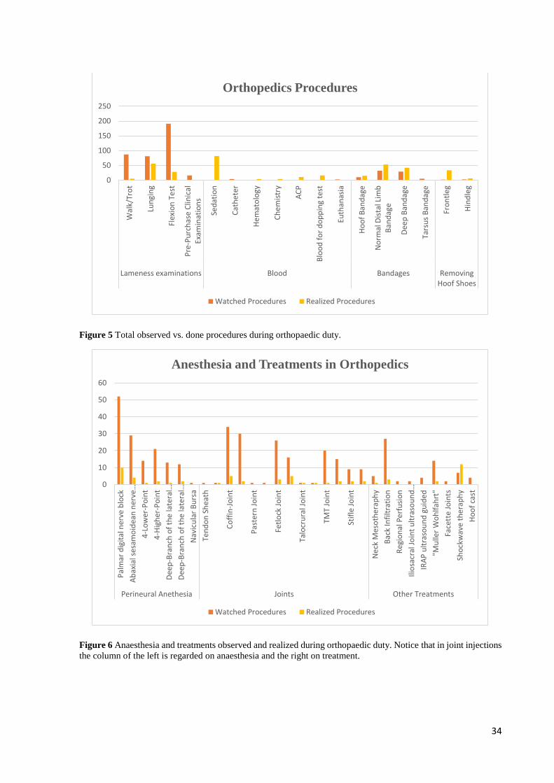
Figure 5 Total observed vs. done procedures during orthopaedic duty. .................................. 34
Figure 6 Anaesthesia and treatments observed and realized during orthopaedic duty. ........... 34
Figure 7 Imaging procedures watched and realized during orthopaedic duty. ........................ 35
Figure 8 GRE Pulse sequence Family Tree. ............................................................................ 38
Figure 9 SE and FSE Pulse Sequence Family Tree. ................................................................ 38
Figure 10 MRI Artefacts. ......................................................................................................... 45
Figure 11 X- Ray set from the hoof in a horse with a positive palmar digital nerve anesthesia.
.................................................................................................................................................. 52
Figure 12 Ultrasound of the PTA. ........................................................................................... 53
Figure 13 Sagittal (A) and Transverse (B) ultrasound scans from the PTA using the transcuneal
approach.................................................................................................................................... 53
Figure 14 Podotrochlear apparatus. ........................................................................................ 56
Figure 15 MRI Findings in the navicular bone. ....................................................................... 59
Figure 16 Lesion DSIL. .......................................................................................................... 60
Figure 17 Lesion DDFT. ......................................................................................................... 61
Figure 18 Lesion DIP Joint. ..................................................................................................... 62
Figure 19 Lesion collateral ligaments of the DIP joint ........................................................... 63
Figure 20 MRI findings in the middle and distal phalax. ........................................................ 63
Figure 21 Sex distribution in the sample. ................................................................................ 65
Figure 22 Distribution of the lameness: Unilateral vs. Bilateral ............................................. 65
Figure 23 Breed distribution in the sample ............................................................................. 66
Figure 24 Prevalence of lesions found in the MRI. ................................................................. 67
Figure 25 DSIL lesions in unilateral and bilateral lameness. .................................................. 68
Figure 26 DDFT lesions in unilateral and bilateral lameness.................................................. 68
Figure 27 Coffin-joint lesions in unilateral and bilateral lameness. ........................................ 68
Figure 28 MRI findings in the navicular bone......................................................................... 70

29
I- EXTERNSHIP
My final curricular externship to obtain the Master Degree in Veterinary Medicine
from FMV-ULHT, was made in the Pferdeklinik Leichlingen GmbH, in Germany, under
supervision of Dr. Klaus-Peter Neuberg and Dra. Juliane Veh.
The externship was carried between the 28 September 2015 and 1st April 2016,
approximately 6 months of duration. In the first 2 months, I had a rotative schedule within the
hospital wich included daily routine practice as well as nightshifts. In this initial 2 months
period I developed a strong interest in sports horse medicine, orthopedics and diagnostic
imaging. To further deepen my interest in this subjects, I was given the opportunity to work
with and support Dr. Neuberg in the Orthopedic department for the rest of my Externship. I was
assisting during the daily routine in a busy hospital with a high orthopedic caseload. Orthopedic
work included normal day orthopedic referral appointments, lameness examinations and pre-
purchase examinations, weekend-shifts and stable visits as well lameness investigation in
hospitalized horses and x-ray duty.
Every Thursday we had a Journal Club in which we discussed a special clinical case,
scientific articles or a chapter of the Equine Surgery Book. All of the procedures were carried
under supervision of a board certified veterinary surgeon.
1. Pferdeklinik Leichlingen
The Pferdeklinik Leichlingen was founded in 2011 by Dr. Björn Nolting, Dr. Matthias
Krebs and Dr. Guido von Plato, and is located between Düsseldorf and Cologne, in Germany.
The hospital provides referral and first opinion service and covers all aspects of modern equine
medicine such as Orthopedics, Sports Medicine and Diagnostic Imaging, Internal Medicine,
intensive Care and Emergencies as well Surgery.
The hospital is divided into different sections. The main building contains the
receptions desk and waittting room, pharmacy and administrative offices and is connected to
the emergency room. In the emergency room where receive all the emergencies, despite cases
suspitions of infectious disease, is equipped with a stock 1 ultrasound machine and a portable
x-ray machine. The laboratory is directly connected to the surgery room. Just next door to the
emergency room is close is the intensive care stable that houses 16 boxes, with 2 foal boxes and
2 stallion boxes.
30
The orthopedic building has 5 examination rooms, 3 ultrasound machines, 1 x-ray
room with a non-portable x-ray machine, and 1 MRI room. Outside there are two trot up strips,
a circle with firm sand for lunging on hard ground as well as a sand school outdoor arena, used
for ridding and lameness or pre-purchase examinations.
The Internal medicine building has 2 big rooms in which one has one stock used for
endoscopy and standing surgeries and the other normally is reserved for dentistry.
The hospital still has 2 more stables each one with 16 boxes, a isolation unit with 6
boxes and a nuclear scintigraphy building with 8 boxes and an outside grazing area for
hospitalized horses, and another barn. The barn there is a indoor lunging circle with soft sand
and another 8 boxes.
2. Casuistry of Externship
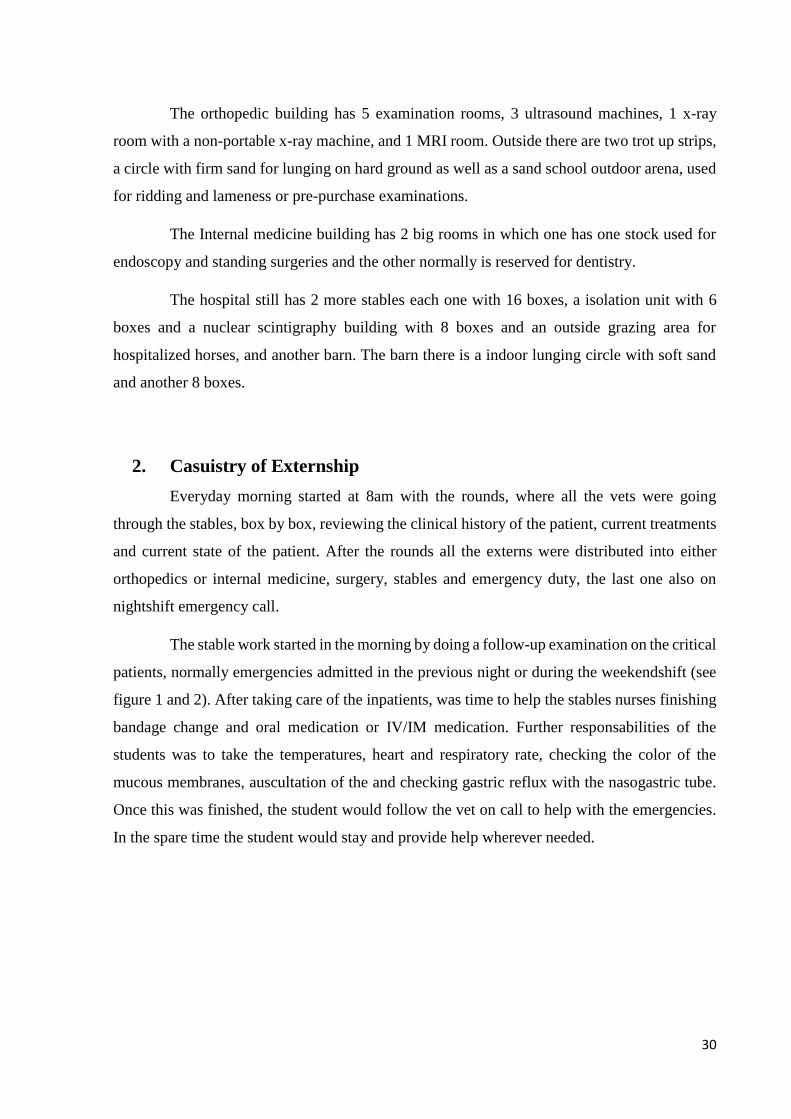
Everyday morning started at 8am with the rounds, where all the vets were going
through the stables, box by box, reviewing the clinical history of the patient, current treatments
and current state of the patient. After the rounds all the externs were distributed into either
orthopedics or internal medicine, surgery, stables and emergency duty, the last one also on
nightshift emergency call.
The stable work started in the morning by doing a follow-up examination on the critical
patients, normally emergencies admitted in the previous night or during the weekendshift (see
figure 1 and 2). After taking care of the inpatients, was time to help the stables nurses finishing
bandage change and oral medication or IV/IM medication. Further responsabilities of the
students was to take the temperatures, heart and respiratory rate, checking the color of the
mucous membranes, auscultation of the and checking gastric reflux with the nasogastric tube.
Once this was finished, the student would follow the vet on call to help with the emergencies.
In the spare time the student would stay and provide help wherever needed.

31
Figure 1 Emergencies cases during weekend and nightshift duty
Figure 2 Total of procedures observed vs. done during weekend and nightshift duty.
While on surgery duty (see figure 3), we started in the morning with a breef clinical
examination of all surgical candidates for the day. Before going into the knock-down-box the
horses were prepared by flushing the mouth with water, putting the stables bandages in all four
0
5
10
15
20
25
30
35
40
45
Lam
init
is
Ho
of
Ab
cess
Cel
ulit
is
Wo
un
ds
Co
lic
An
ore
xy
Dia
rrh
ea
Feve
r
Ata
xy
Swea
llin
g P
rep
uci
um
Ch
oke
Foal
s
Orthopedics Internal Medicine
Weekend and Nightshift Emergencys
0
20
40
60
80
100
120
140
Weekend and Nightshift Procedures
Watched Procedures Realized Procedures

32
legs and in colic patients a nasogastric tube was placed. In the knock-down-box there as usually
four people to anesthetize the horse. When the horse is oin the floor, the anesthetist puts the
endotraqueal tube in and the horse is lifted with a crain on to the surgery table. Depending on
the type of surgery the horse can be positioned right or left lateral recumbency or dorsal
recumbency. After its properly positioned, the surgical field is prepared and the nurses start
scrubbing with chlorhexidine solution followed by 70% alcoohol. During the surgery it self, the
student would either watch the surgeon, assisting the surgeon if necessary or help with the
anesthesia. Afterwards the student would help to recover the horse, while the anesthetist would
knock the next horse out and keep going. On a routine day the hospital would operate and
average from 5 to 7 horses.
Figure 3 Total of surgeries and surgical field preparations during surgery duty.
While on the Internal Medicine department (see figure 4), the day also started by making
a “to do” list of all the in patients, and normally included endoscopy as well as helping the
stables vet with emergencies and also laboratory work. Normally the first appiotments would
start before lunchtime.
0
10
20
30
40
50
60
Surgery
Surgery Surgical field preparation

33
Figure 4 Total of cases and procedures during internal medicine duty. *Liver and lung biopsy.
As mentioned before, I spent almost 3 months in Orthopedics were I was mostly
assinting Dr. Neuber and occasionally other vets. After the rounds, the student would start the
day by checking the list of all the appointments throughout the day and out to fit the inpatients
in between them. Depending on how busy the day was going to be, the day was started with
appointments or with inpatients. The student responsability was to constantly assist the vet
thought the day and discussing every case. In the early stages of the externship in orthopedics
the student started by assisting in basic things such as to trot the horses up and lounging them,
scrumbing for nerve blocks and sterile joint injections, preparing ultrasounds and process blood
samples in the laboratory. As time went on, the student was allowed to do all types of medical
procedures, like perineural anesthesia, joint injections and ultrasounds, always
undersupervision of Dr. Neuberg (see figure 6 and 7). In Orthopedics, there was a chance to see
the most variety of cases and choice of treatments or procedures and specially to see follow up
examinations and the course of recovery in every case (see figure 5).
0
5
10
15
20
25
30H
eart
Ult
raso
un
d
Hea
rth
X-R
ays
Ch
eck
Pre
gnan
cy c
on
tro
l
Ch
eck
Teet
h E
xtra
ctio
n
Man
dib
ula
r fr
actu
res
Ch
eck
Gas
tro
sco
py
Lari
ngo
sco
py
Bro
nch
osc
op
y
Gu
tura
l Po
uch
es
Fist
ula
(Te
eth
)
Frac
ture
s M
and
ibu
la (
Ce
rcla
ge f
ixat
ion
)
Surg
ery
pre
-ch
eck
Hem
ato
logy
Ch
esm
istr
y
Bio
psy
*
Rec
tal E
xam
inat
ion
Ab
do
min
alce
nte
sis
Ab
do
min
al u
ltra
sou
nd
Lun
ge U
ltra
sou
nd
Lun
ge/
Traq
ue
a x-
ray
Hea
d x
-ray
Cardiology Gineacology Dentistry Endoscopy Surgery Diagnostic
Internal Medicine
Watched Procedures Realized Procedures
34
Figure 5 Total observed vs. done procedures during orthopaedic duty.
Figure 6 Anaesthesia and treatments observed and realized during orthopaedic duty. Notice that in joint injections
the column of the left is regarded on anaesthesia and the right on treatment.
0
50
100
150
200
250
Wal
k/Tr
ot
Lun
gin
g
Flex
ion
Te
st
Pre
-Pu
rch
ase
Clin
ical
Exam
inat
ion
s
Sed
atio
n
Cat
he
ter
Hem
ato
logy
Ch
em
istr
y
AC
P
Blo
od
fo
r d
op
pin
g te
st
Euth
anas
ia
Ho
of
Ban
dag
e
No
rmal
Dis
tal L
imb
Ban
dag
e
Dee
p B
and
age
Tars
us
Ban
dag
e
Fro
ntl
eg
Hin
dle
g
Lameness examinations Blood Bandages RemovingHoof Shoes
Orthopedics Procedures
Watched Procedures Realized Procedures
0
10
20
30
40
50
60
Pal
mar
dig
ital
ner
ve b
lock
Ab
axia
l ses
amo
idea
n n
erve
…
4-L
ow
er-P
oin
t
4-H
igh
er-P
oin
t
Dee
p-B
ran
ch o
f th
e la
tera
l…
Dee
p-B
ran
ch o
f th
e la
tera
l…
Nav
icu
lar
Bu
rsa
Ten
do
n S
hea
th
Co
ffin
-Jo
int
Pas
tern
Jo
int
Fetl
ock
Jo
int
Talo
cru
ral J
oin
t
TMT
Join
t
Stif
le J
oin
t
Ne
ck M
eso
the
rap
hy
Bac
k In
filt
rati
on
Reg
ion
al P
erf
usi
on
Ilio
sacr
al J
oin
t u
ltra
sou
nd
…
IRA
P u
ltra
sou
nd
gu
ided
"Mu
ller
Wo
hlf
ahrt
"
Face
tte
Join
ts
Sho
ckw
ave
the
rap
hy
Ho
of
cast
Perineural Anethesia Joints Other Treatments
Anesthesia and Treatments in Orthopedics
Watched Procedures Realized Procedures

35
Figure 7 Imaging procedures watched and realized during orthopaedic duty.
0
5
10
15
20
25
30
35
40
45
Pas
tern
Fetl
ock
Can
on
Bo
ne/
Ten
do
n S
hea
th
Stif
le
Car
pu
s an
d c
arp
al t
un
nel
Tars
us
and
ten
do
n s
he
ath
Ilio
sacr
al J
oin
t
Ne
ck a
nd
nu
ca
Dis
tal L
imb
s
Car
pu
s
Tars
us
Can
on
Bo
ne
Splin
t B
on
es
Elb
ow
Sho
uld
er
Stif
le
Bac
k
Ne
ck
Hip
Lun
gs
Max
ila
Man
dib
ula
Inci
sivs
Tem
po
rom
and
ibu
lar
Join
t
Pre
-Pu
rch
ase
exa
min
atio
n
Ultrasound X-Rays
Imaging Procedures in Orthopedics
Watched Procedures Realized Procedures
36
II- LOW-FIELD MRI IN PODOTROCHLEOSIS
1. Introduction
MRI is a diagnostic imaging modality that depends on the distribution and
concentration of hydrogen nuclei in biological tissue, its properties and how each nuclei reacts
and resonates in the presence of a magnetic field (Labruyère & Schwarz, 2013; Lauterbur,
1973). Hydrogen is among the most sensitive nuclei to a magnetic field gradient and it is a
nuclei with natural abundance in biological tissue, making possible the creation of images with
no need to expose or add any other substance (Armstrong & Stephen, 1991).
When a magnetic field is applied to hydrogen protons, the MRI can create an image
by detecting the signal of these protons in the water and fat of biological tissues (Armstrong &
Stephen, 1991; Damadian, 1971; Lauterbur, 1973).
This is accomplished by placing the part of the limb to be imaged within a magnetic
field and to subject it to perturbing radiofrequency pulses (Armstrong & Stephen, 1991;
Labruyère & Schwarz, 2013). Magnetic resonance signal intensity vary widely in different
musculoskeletal tissues, due to differences in proton density and status of the chemically free
versus bound hydrogen nuclei, and for that reason, different tissues will appear differently in
the same image or scan (Armstrong, 1991). Applying a linear magnetic field i.e. a magnetic
field stronger on one side, the position of the nuclei can be determined by measuring the
resonance frequency. Because they are in different position in the field gradient, they resonate
in different frequencies (Armstrong & Stephen, 1991; Lauterbur, 1973).
Magnetic resonance signal can be detected from a wide range of nuclei, but as
explained above, only hydrogen nuclei are used because of their unique benefits, and the term
“nuclear” was dropped and the abbreviation MRI was used ever since (Armstrong & Stephen,
1991; Murray, 2011).
1.1. Basics of MRI
Magnetic resonance images depend on the absorption of radio-waves (radiofrequency
pulses) by hydrogen nuclei. The radiofrequency (RF) pulses are transmitted to the patient by a
RF transmitter coil and absorbed by hydrogen nuclei. The nuclei gain energy and reemit this
energy through RF signal wich is detected by a RF receiver coil (Armstrong & Stephen, 1991).
37
The size of the RF signal will depend on proton density i.e. the number of hydrogen nuclei in
the tissue, T1 and T2 relaxation times (Armstrong & Stephen, 1991; Murray, 2001). T1 and T2
relaxation times reflect the rate at which excited protons lose their energy (Armstrong &
Stephen, 1991). Every MR image contains both T1 and T2 information, but by choosing the
appropriate timing and length of the RF pulses, the images can depend mainly on one or the
other (Armstrong & Stephen, 1991). Different combinations of RF pulses and magnetic fields
can be used to create sequences of images with different contrasts (Labruyère & Schwarz,
2013).
The body part of interest has to be placed into a magnetic field. The stronger the
magnetic field, the greater the proportion of nuclei that will line up in the direction of the field,
and the stronger the signal will be received (Armstrong & Stephen, 1991; Murray, 2001). In
low-field, standing MRI, usually, it is used a 0,27T field strength. Since the spatial origin of the
signals can be localised, an image can be created (Armstrong & Stephen, 1991; Lauterbur,
1973).
In terms of physics, the nucleus of each atom is electrically positive due to the presence
of charge carrying-protons (Murray, 2001). Besides these properties, neutrons and protons have
another physical property called spin, that gives rise to the phenomenon of nuclear magnetic
resonance (NMR). (Armstrong & Stephen, 1991; Murray, 2011).
When the patient is placed into the magnet, the nuclei in the biological tissue will line
up with the direction of the field (Armstrong & Stephen, 1991; Murray, 2011). RF pulses
transmitted cause some protons to alter their alignment relative to the field. Once the RF coil is
turned off the protons return to their original equilibrium, accompanied by a release of energy
in the form of a RF signal, which will be captured by a receiver coil (Labruyère & Schwarz,
2013).
T1 relaxation time represents the rate at which the excited protons realign with the
field, after the transmitter RF coil is turned off (Armstrong & Stephen, 1991; Labruyère &
Schwarz, 2013). In MRI, the RF pulses excite the protons to a higher energy state but also put
them in to phase. When the pulse is turned off, the protons start to dephase. T2 is a relaxation
time, that reflects the rate of signal decay due to dephasing of the spinning protons (Armstrong
& Stephen, 1991).

38
In biological tissue, T1 is faster in fat and slower in fluid/water and this can be used to
distinguish both of them on images. By applying pulses in quick succession, the water nuclei
never get a chance to recover, contrary to the fat nuclei that do so repeatedly and generate a
strong signal. (Damadian, 1971; Damadian et al, 1974; Murray, 2011)
T2 relaxation is sensitive to the degree of mobility of a substance, being much longer
in fluids and shorter in solid material and also being extremely sensitive to the external
environment (Murray, 2011).
As mentioned above, pulse sequences can be defined to create images with different
contrasts (Labruyère & Schwarz, 2013). A pulse sequence are usually repeated many times
during a scan, whereareas the time interval between pulses and the amplitude and the shape of
the gradient waveforms will control the signal reception and affect the characteristics of the
MR images. Computer programs that control all hardware aspects of the MRI measurement
process drive pulse sequences. Gradient-Echo (GRE) and Spin-Echo (SE) are the two different
types, that are used most frequently (MR- Technology Information Portal, 2003; Murray, 2001).
Figure 8 GRE Pulse sequence Family Tree (Adapted from Hallmarq Veterinary Imaging, 2011)
Figure 9 SE and FSE Pulse Sequence Family Tree (Adapted fromHallmarq Veterinary Imaging, 2011).
Gradient Echo (GRE)
Pilot scans
T1 GRE (2D)
T1 3D + T1 3D
Isotropic
T2* GRE + T2W GRE
T2* 3D + T2W 3D
T2 Isotropic
STIR GRE
Spin Echo (SE)/ Fast Spin Echo (FSE) - 2D only
T1 SEPD SE + PD
FSEDual Echo
T2 FSE
STIR TEST
STIR FSE

39
The signal to noise ratio (SNR) is used in MRI to describe the relative contributions
of a detected signal to the true signal and to random superimposed signals ('background noise')
- a criteria for image quality (MR- Technology Information Portal, 2003; Murray, 2001).
GRE sequences have a higher signal to noise ratio and lower T2W contrast when
compared to SE that have higher T2W contrast and lower signal to noise ratio. For that reason,
SE sequences can have poorer image quality, when compared to GRE sequences, and
necessitate reduced spatial resolution and increased slice thickness. GRE sequences are more
susceptible to some artifacts and are more useful to obtain high anatomic resolution images and
T1W images of bone (Murray, 2001).
GRE SE/ FSE
Fast imaging sequences Slower sequences
Less sensitive to patient motion More sensitive to patient motion
High relative SNR Lower relative SNR
Less image contrast Greater image contrast
Sensitive to magnetic field distortions –
signal “drop out”
Relatively insensitive to magnetic field
distortions
Fat/water cancellation artefacts can occur Less susceptible to image artifacts
Mix of T1W and T2*W contrast Image contrast is easier to understand
2D or 3D scans 2D scans only
Table 1 Differences between GRE and SE/FSE (Adapted from Hallmarq Veterinary Imaging, 2011).
1.2. MRI Safety, Equipment and Facilities
Although MRI practice does not carry hazards like some other modalities in imaging
such as radiology and scintigraphy (Labruyère & Schwarz, 2013; Mair et al., 2005), there are
still some health and safety issues that should be avoided and minimised. Warning signs should
be positioned both on the front MRI door and inside. The MRI room should have restricted
access, and should be entered through a lockable door only (MR- Technology Information
Portal, 2003; Murray, 2001). All ferromagnetic objects including medical equipment such as
scalpelsblades and clippers, will be attracted to the magnet, this may cause issues for the
technicians or the horse and, if used too close can cause a magnetic field disruption, resulting
in image artifacts (Hartwig et al., 2009; Murray, 2011). To scan the hoof region, the hoof-shoes

40
have be removed before hands, and a dorsoproximal-palmarodistal x-ray picture should be
taken prior to the scan, to make sure there are no nail pieces left, that may cause artifacts
(Murray, 2001). It is essential that no metallic object are allowed to enter the MRI room, this
includes personal objects of the technicians like watches, mobile phones, coins and jewelry.
The same is applied to all magnetic material implanted into the horse or patient such as
pacemakers or other metallic implants that can have their function disrupted (Hartwig et al.,
2009; MR- Technology Information Portal, 2003; Murray, 2011).
1.3. Image Interpretation
The MR images are produced in a grey scale with a varying range of contrasts that are
a result of the level of signal intensity (Mair et al., 2005). The appearance of a tissue on the
image is affected by its nature, by the system, pulse sequence and acquisition parameters
(Armstrong & Stephen, 1991; Labruyère & Schwarz, 2013). When a tissue is injured, changes
in the tissue structure, biochemical composition or water distribution result in alterations in the
MR images appearance (Murray, 2011).
The signal comes mainly from the mobile hydrogen protons present in fat and water
(Armstrong & Stephen, 1991) and that is why structures that have just a few or no free hydrogen
protons appear black (Mair et al., 2005; Murray, 2001). The contrast in the images can be
determined by Proton Density (PD), T1 and T2 properties (Armstrong & Stephen, 1991) and
by manipulating the pulse sequences, and for that reason a tissue has different appearances on
T1, T2 and PD images (Labruyère & Schwarz, 2013; Murray, 2001). For images referred as T1
or T1-weighted, contrast is dependent mainly on T1 relaxation properties, for T2 or T2-
weighted, the contrast is dependent on T2 relaxation properties and PD or PD-weighted the
contrast is dependent on the proton density i.e. the number of free and mobile hydrogen nuclei
in the tissue (Murray, 2011).
Fluids have long T1 relaxation time but it is very short in fat-based tissues. On T1W
images water based tissues will appear in a mid-grey scale, depending on the water content as
with more water on the tissue the image becomes darker. Tissue with higher water content due
to edema or increased capillary content will appear darker than the surrounding normal tissue.
Fat based tissues, on T1W images will appear brighter (Murray, 2011). T1W provides the best
anatomical detail and for this reason is considered the standard accepted sequence for baseline
information of the musculoskeletal system (Mair et al., 2005).
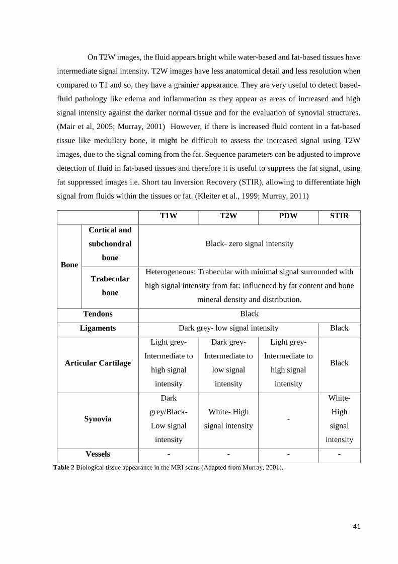
41
On T2W images, the fluid appears bright while water-based and fat-based tissues have
intermediate signal intensity. T2W images have less anatomical detail and less resolution when
compared to T1 and so, they have a grainier appearance. They are very useful to detect based-
fluid pathology like edema and inflammation as they appear as areas of increased and high
signal intensity against the darker normal tissue and for the evaluation of synovial structures.
(Mair et al, 2005; Murray, 2001) However, if there is increased fluid content in a fat-based
tissue like medullary bone, it might be difficult to assess the increased signal using T2W
images, due to the signal coming from the fat. Sequence parameters can be adjusted to improve
detection of fluid in fat-based tissues and therefore it is useful to suppress the fat signal, using
fat suppressed images i.e. Short tau Inversion Recovery (STIR), allowing to differentiate high
signal from fluids within the tissues or fat. (Kleiter et al., 1999; Murray, 2011)
T1W T2W PDW STIR
Bone
Cortical and
subchondral
bone
Black- zero signal intensity
Trabecular
bone
Heterogeneous: Trabecular with minimal signal surrounded with
high signal intensity from fat: Influenced by fat content and bone
mineral density and distribution.
Tendons Black
Ligaments Dark grey- low signal intensity Black
Articular Cartilage
Light grey-
Intermediate to
high signal
intensity
Dark grey-
Intermediate to
low signal
intensity
Light grey-
Intermediate to
high signal
intensity
Black
Synovia
Dark
grey/Black-
Low signal
intensity
White- High
signal intensity -
White-
High
signal
intensity
Vessels - - - -
Table 2 Biological tissue appearance in the MRI scans (Adapted from Murray, 2001).

42
As described above, STIR scans are a form of fat suppression that allows any
underlying fluid signal to be seen by suppressing the fat signal (Mair et al., 2005; Murray,
2001). STIR scans can be both GRE or FSE (Hallmarq, 2011).
1.4. Image Quality and Artifacts
Image quality is determined by signal, noise, contrast and artefacts, but signal, and
noise are often considered together as the signal to noise ratio (SNR) (Murray, 2011).
1.4.1. Signal
The MR signal comes from the hydrogen nuclei within the biological tissue. Increased
field strength and increased amounts of material, give more signal but this is sharply reduced
as the image resolution increases (Murray; 2011).
1.4.2. Noise
Electrical noise is generated by thermal motion of electrons in the sample, coil and
amplifiers and care should be taken not to allow any external sources of noise to further degrade
the image quality (Murray, 2011).
1.4.3. Contrast
If images were with no contrast at all and all tissues of the same grey intensity, they
wouldn’t have any diagnostic value. The contrast of the images comes from the different
amount of signal (proton density) within the different tissues but for diagnostic interpretation a
greater contrast is obtained at lower signal strengths. So normally, GRE images have more
signal but less contrast and on the other hand, SE images have more contrast but less signal
(Murray, 2011).
1.4.4. Artefacts
Artifacts is the term for everything in an image, that does not truly represented what is
being imaged. The dilemma of an artifact is that it can be interpreted as a pathologic finding
and, therefore, can lead to a false diagnosis. Artifacts do occur commonly. They can be caused
by patient related factors, acquision technique, nature of the MRI and also due to imperfections
in the system. They are classified into motion artifacts, magnetic field inhomogeneity and
digital imaging artifacts (Murray, 2011). The artifacts are:
1. Motion artifacts: Are caused by movement during scans acquisition, including
involuntary movements such as breathing, pulsatile movement in the vessels and blood
43
flow, or small movements in over sedated horses. This results in a smearing or blurring
and ghosting of the scans. Continuous movement of the area to be scanned can lead to
a non-diagnostic scan. This can be minimised by using motion insensitive (MI) scans,
as these allow the system to acquire the data only when the horse is stationary by
repositioning of the slices when motion is detected and acquirement of segments in real
time, but this lead to longer scans acquisition time. Other option is to use fast or super-
fast scans (Murray, 2011).
2. Magnetic field inhomogeneity artifacts: It is mandatory to have a homogeneous
magnetic field, in order to obtain a good quality in MR images. A heterogeneous field
often leads to artifacts and is normally caused by temperature fluctuations and metal.
Metal artifacts are seen as an area of zero signal within a high intensity rim and distortion
in adjacent tissues. Metal artifacts are more severe in GRE scans than in SE. In order to
minimise these artifacts, temperature and humidity should be controlled inside the MRI
room, and it is also important that all the metal is removed within the magnet area, shoes
and nails included. It is advised to take a dorsoproximal-palmarodistal x-ray view prior
to the scan, to look for any nail fragments after shoe removal as they can produce severe
metal artifacts. Steel toecap boots should also be avoided in the area near the magnet.
Hemosiderin artifact will appear as a black region on the image that can be useful to
determine the extension of a penetrating injury (Murray, 2011).
3. Fat/Water Cancellation: The resonant frequency of fat and water are different, at the
time the echo is collected. On T2* and T2W, both expected to show increased brightness
associated with increased fluid water content. This is the basis for their diagnostic use
in detecting edema and inflammation. Sometimes, the areas that appear bright in T2W
FSE, can appear dark in T2*W GRE, and this is due to the signal from fat and water
cancelling each other out. This phenomenon occurs in injured bone, where fluid and fat
can both occupy the trabecular spaces. The true presence of water can be determined by
using STIR sequence, but care must be taken not to misdiagnose the lesion as sclerosis.
(Hallmarq Veterinary imaging, 2007) If true sclerosis is seen, it should appear as a low
signal in all the sequences and on the other way fluid should appear with low signal on
T1 GRE but with high signal in STIR, Proton Density (PD) and T2 FSE. (Murray, 2011)
The T2*GRE may be also helpful in detecting fluid as fat/water cancellation does not
happen when the amount of fluid is bigger than the fat. (Murray, 2011).

44
4. Magic angle effect: When collagen fibers of tendons and ligaments are aligned at the
particular angle of 54.7° (+/- 10°) to the main magnetic field, the T2 relaxation increases.
Normally the T2 relaxation of normal tendon tissue is so fast, that the signal is gone
before it is collected and it is for that reason, that it appears dark. When the tendon is
aligned at the “magic angle”, the signal duration is increased and the tissue will have an
artefactual increased signal and will appear grey, which can be mistaken as pathology.
The magic angle effect is reduced as TE increases, so T2W FSE images are less,
susceptible while T1W and PDW are more susceptible because of their short TE. In the
low field standing MRI, it is often seen in the collateral ligaments of the DIPJ, oblique
sesamoidean ligaments, abaxial aspect of DDFT and in the distal annular ligament. It is
more likely to occur in the lateral collateral ligament, lateral lobe of the DDFT and
medial oblique sesamoidean ligament in the standing horse with the limb slightly
abducted, which is the most common position while scanning. It is recommended for
this reason, that the horse stands as squarely as possible in order to minimise magic
angle effect. Limb repositioning in the magnetic field should also be taken as an option
(Murray, 2011);
5. Partial volume effect: This occurs when a mixture of different tissue types is in the
same voxel, causing misleading pixel intensities in the images. When curved or irregular
T1
GRE PDW T2*W GRE T2W FSE STIR
Sclerosis Low
signal Low Signal Low signal Low signal Low signal
Fluid
(edema)
Low
signal
Intermediate
to high signal
Intermediate
to high signal
Intermediate
to high signal
Intermediate
to high signal
Phase
Cancellation
(Water =
Fat)
- - Low signal High signal High signal
Table 3 Appearance of phase cancellation artefact in the different pulse sequences and its difference to bone
edema and sclerosis appearance (Murray, 2001)

45
shaped surfaces or edges are scanned and parts of more than one structure appear in the
same slice in apposition, or even when they are partially cross, cut between or separated
into two different slices, the margins tend to appear less clearly defined and small
structures may be missed completely. By reducing the slice thickness, the effect is also
reduced but as the SNR is reduced, the imaging time increases. Using a combination of
sequences, including HR scans over the area of interest, might also be beneficial. For
curved articular surfaces, it is useful to acquire the images perpendicular to the articular
surface in several points across the joint (Murray, 2011);
6. Temperature effects: System parameters and image appearance can be affected by the
temperature of the magnet but also by the temperature of the tissues. This has more
impact when STIR sequences are being used because the optimal inversion time for fat
suppression or fluid attenuation is affected by the temperature. It is advised to take a
STIR test to find the optimal inversion time (Murray, 2011).
Figure 10 MRI Artefacts. From the left to the right the first picture represents the “noise” caused by a
heterogeneous magnetic field due to temperature floatation. The second picture represents a motion artefact from
the blood vessels. The third and fourth pictures a heterogeneous magnetic field due to radiofrequency interference
and a piece of metal from a nail, respectively.
1.5. Clinical Approach to the Lame Horse
1.5.1. Anamnesis
Clinical history, should be taken to obtain basic information such as age of the horse,
sex, breed and use, and additional information with questions tailored to the specific patient
(Ross & Dyson, 2003). An accurate history is an essential step in attempting to identify the
cause of a poor athletic performance or lameness (Hinchcliff et al., 2004).
Many pathologies are age-related and some problems also can get worse with
advancing age (Ross & Dyson, 2003). There are however situations, when attempting to acquire
an accurate history is a true challenge (Moyer, 2010). It is very important to directly ask the

46
owner about the duration and nature of the problem, if it gets better or worse with exercise and
how the problem was managed or treated so far (Moyer, 2010; Ross & Dyson, 2003).
Asking questions in a nonthreatening fashion and avoiding a condescending or
sarcastic manner is essential.
The role of the veterinarian is to collect as many information as possible, particularly
whether the problem is complex or not apparent (Hinchcliff et al., 2004).
Anamnesis: Basic and specific information
Signalment
Age
Sex
Breed
Use: Competitive activities such as Jumping or Dressage have a
subset of predictable/common injuries. Level of competition
Current
Lameness
What is the
problem?
History of trauma
Duration of lameness
Deterioration or improvement of lameness and its circumstances
Exercise effect on the lameness
Past lameness problems
Management
Changes
Changes in shoeing
Changes in training or performance intensity
Changes in surface
Changes in diet and health
Changes in housing
Current medication and response
Specific
information
Type of sporting activity and level of competition
Others:
Videotapes
Images
Records
Clinical records from other clinic/hospital
Discussions with others
Table 4 Information to be included in the anamnesis (Ross & Dyson, 2003).

47
Navicular disease is recognised in horses with a wide variety of hoof shapes like the
Quarter Horse with narrow and boxy upright feet, Thoroughbreds with flat hoofs and low and
collapsed heels and European Warmbloods (Dyson et al., 2010; Waguespack & Hanson, 2010).
In case of poor hoof conformation, it is worthwhile improving the trimming and shoeing and
re-assessing the lameness after several weeks and if the lameness has markedly improved, it is
unlikely to be a navicular problem. (Ross & Dyson, 2003)
1.5.2. Physical Examination
The lameness examination should always begin with the observation of the horse,
standing in a square position. (Ross & Dyson, 2003) It is very important at this stage to check
from the distance, if there is any muscle asymmetry, areas of swelling and to look for the
symmetry of the limbs, as well for limb conformation and hoof configuration (Auer & Stick,
1999; Hinchcliff et al., 2004). Palpation of the vertebra begins at the poll, continues down the
length of the cervical spine and ends with palpation of the withers. Limb palpation begins in
the front limbs at the level of the scapula and continues down until the hoof. The entire length
of the limb is palpated to include the weight-bearing surface of the foot and the shoe (Moyer,
2010). The degree of digital pressure might vary, but with the initial palpation we try to
appreciate differences like atrophy, swelling or heat. This is followed by applying increased
digital pressure to detect the presence or absence of pain (Auer & Stick, 1999; Ross & Dyson,
2003). The veterinarian should palpate, feel and manipulate every possible anatomical
structure, like soft tissue, i.e. muscles, tendons, ligaments and joints. If any finding or doubt, it
should be compared with the contralateral limb, always bearing in mind that both sides might
be affected (Moyer, 2010). In normal horses, digital pulse may be difficult to detect, especially
in cold weather, and so if it is with increased strength, it can be a sign of inflammatory
conditions like hoof abscess or laminitis. (Ross & Dyson, 2003)
Examination of the hoof is accomplished by cleaning the sole and the frog with a hoof
pick or with a hoof knife. Removal of the shoe is indicated, when a sub-solar abscess is
suspected (Moyer, 2010; Ross & Dyson, 2003). When the hoof is prepared, it should be
carefully examined with hoof testers. The veterinary should hold the hoof between the legs and
must be able to feel the horses reactions to subtle pressure.
Examination is continued to evaluate the length of the back beginning at the withers
and ending with the tail head. The initial assessment is followed by more aggressive digital

48
pressure to appreciate presence or absence of pain, muscle atrophy and symmetry (Ross &
Dyson, 2003). The pelvis and pelvic musculature is then palpated with the horse standing as
squarely as possible (Moyer, 2010). All the bony protuberances should be palpated, including
tubera coxae, tubera sacrale and tubera ischia, by standing behind the horse and palpating both
sides simultaneously (Ross & Dyson, 2003). After that the hip and thigh region is palpated and
manipulated followed by palpation of the stifle. Distal limb palpation mirrors the technique
utilized with the forelimbs (Moyer, 2010; Ross & Dyson, 2003).
1.5.3. Examination in Motion
After examination of horse at rest is completed, dynamic examination should be
performed. The horse should be observed at first in a straight line at walk and trot on hard
surface (Auer & Stick, 1999). Here it is important to note the synchrony, symmetry and
pathway of the limb swing and how each hoof contacts the ground (Auer & Stick, 1999;
Hinchcliff et al., 2004). Each foot should normally land heel first, then toe with the lateral and
medial aspects of the hoof nearly equally in time. Deviations from normal footfall may indicate
dynamic imbalance of the limb that could be due to abnormalities of conformation (Ross &
Dyson, 2003). The horse should be trotted in a straight line, away from and toward the
veterinarian, followed by in hand trotting on a circle on both right and left reign (Moyer, 2010).
Afterwards the horse should also be worked in a lounge line in walk, trot and canter on soft
ground, to observe the effects of differential loading between the inside and outside limbs
(Hinchcliff et al., 2004; Moyer, 2010; Ross & Dyson, 2003). Cantering or galloping may be
necessary to appreciate the lameness. The motion examination should be performed on both
soft and hard ground due to the fact that some lameness’s get worse and more obvious on soft
or on harder ground, depending on the cause (Ross &Dyson, 2003). It is also important to access
if the lameness is worsen with ridden work, because some horses thought to be lame are actually
victims of poor riding technique (Moyer, 2010).
Forelimb lameness is usually easier to identify (Ross & Dyson, 2003) as the head rises
immediately prior to and during weight bearing of the lame limb (head bob), and head dropping
as the sound limb contacts the ground. Hind limb lameness can be seen as elevation of the hip
(“hip hike”), dropping of the hip, toe dragging or decreased stride length, depending on the
nature of the lameness (Auer & Stick, 1999). Severe hind limb lameness is often associated

49
with head bob in the contralateral front limb, due to weight shifting to the front (Hinchcliff et
al., 2004; Ross & Dyson, 2003)
The lame limb is identified and the lameness is scored by its severity:
After determining the affected limb and the degree of lameness by watching the horse
in motion, identification of the region of the limb is pursued by manipulation and flexion test
(Auer & Stick, 1999; Moyer, 2010). The flexion tests are used to apply stress or pressure on an
anatomic region of the limb during a period of time with the purpose of lameness exacerbation
(Ross & Dyson, 2003). Following the flexion test, the horse is trotted and the effects of the
flexion on the gait are observed (Hinchcliff et al., 2004). The amount and duration of pressure
applied may affect the outcome, as horses are more likely to manifest a false positive response
as the force increases (Auer & Stick, 1999). Flexion test lack specificity because it is nearly
impossible to flex a single joint without to flex other joints or nearby tissues (Auer & Stick,
1999).
Clinical signs in horses with navicular disease are often first seen between 7 and 9
years of age, although it can occur earlier in age (Waguespack & Hanson, 2010). It is also very
common, that a lameness develops after change of ownership due to the change in trimming
and shoeing associated with different patterns and different periods of working and rest (Moyer,
2010; Ross & Dyson, 2003). Clinical signs in a horse with navicular disease can be extremely
variable. The horse may show a tendency to stumble, associated with a shortening of the stride,
may move better on a soft ground, may have coffin joint distention or even lameness. It is very
common that the horse shows no lameness at all, and the only complain of the owner could be
Grade Lameness scoring
0 Sound;
1 Lameness difficult to observe and not consistently apparent regardless of
circumstances;
2 Mild lameness and consistently apparent under certain circumstances;
3 Obvious lameness observable under all circumstances;
4 Severe lameness with extreme head nod and pelvic hike present;
5 No weight bearing.
Table 5 Quantification of lameness severity (Ross & Dyson, 2003).

50
loss of action, stiffness or unwillingness to jump (Hinchcliff et al., 2004). The response to distal
limb flexion is extremely variable in horses with navicular disease. The lameness is usually
worst on hard surface on a circle with the affected limb on the inside (Waguespack & Hanson,
2010). Often the horse response is negative when pressure is applied into the heels and frog
region, although some authors have described a positive response fairly consistent in horses
with navicular disease (Ross & Dyson, 2003, Waguespack & Hanson, 2010).
1.5.4. Diagnosing Anesthesia
After performing the dinamic examination, regional anesthesia should be performed
to check from which part of the limb the pain arises. Perineural anesthesia should always be
performed from distal to proximal (Moyer, 2010).
The first step is to perform a palmar digital nerve block, using no more than 2ml of
mepivacaine per site, immediately proximal to the cartilages of the foot after palpating the nerve
(Werner, 2013). The lameness is likely to improve in horses with navicular disease after 8
minutes, though sometimes an abaxial sesamoidean nerve block is necessary to achieve
soundness (Ross & Dyson, 2003). After waiting the 8 minutes, the horse should be re-evaluated
on both straight and circle, to determine if the lameness has improved and if it shifts to the
contralateral limb (Ross & Dyson, 2003; Schramme et al., 2007). In horses with severe
lameness, it is advised to perform lateromedial and dorsopalmar x-rays views of the foot, prior
to blocking, to prevent possible fractures after anesthesia (Auer & Stick, 1999).
For the abaxial sesamoidean nerve block, it should be used no more than 4ml of
mepivacine, 2ml per site, at the base of the sesamoidean bones, below the fetlock joint
Schramme et al., 2015, Werner, 2013).
Typically, perineural anesthesia should first be performed, and after having a positive
response intra-articular anesthesia can be considered. If a horse has a positive response to a
palmar digital nerve or abaxial sesamoidean nerve block, the next step should be performing a
DIPJ block. For that and independent of the approach, the area should be prepared sterile with
chlorhexidine solution, scrubbing for at least 5 minutes and cleaning after with alcohol to avoid
complications associated with sepsis (Auer & Stick, 1999; Werner, 2013). All the material used
to perform this block should be completely sterile, i.e. gloves, needles, syringes, anesthetic drug
bottle (Auer & Stick, 1999). For a coffin joint block, 6ml of mepivacaine its placed inside the
joint, and the horse is re-evaluate after 5 minutes (Ross & Dyson, 2003; Schramme et al., 2015).

51
Navicular bursa anesthesia can also be performed with 3 to 4ml of mepivacaine, and
similar to a coffin joint, the site of injection and material should be prepared in sterile fashion.
It is best performed under radiographic or ultrasonographic control and the needle should be
placed in the middle of the flexor surface of the navicular bone (Ross & Dyson, 2003;
Schramme et al., 2007). Like the DIPJ anesthesia, the horse should be re-evaluated 5min after.
A negative response to anesthesia of the distal limb makes it unlikely that the horse has
navicular disease (Ross & Dyson, 2003).
1.5.5. Diagnostic Imaging
1.5.5.1. Radiographic Examination
After localizing the foot as a source of pain, by clinic examination and diagnostic
anesthesia, radiographs should be taken. To improve the quality of the x-rays and to reduce
scatter, the shoes should be removed and the hoofs properly prepared (Ross & Dyson, 2003;
Butler et al., 2000). It should include at least a lateromedial and dorsopalmar view in weight
bearing position as well dorsoproximal-palmarodistal oblique and palmaroproximal-
palmarodistal views in a hickman-block. Some extra x-rays can be taken like dorsolateral-
palmaromedial and dorsomedial-palmarolateral views (Martinelli & Rantanen, 2002; Widmer
& Fessler, 2002). Packing the sole with playdough will eliminate air shadows that might be
confused with pedal bone fractures. (Butler et al., 2000).
Condition Radiographic findings
Excellent Good corticomedular differentiation with a flexor surface of uniform thickness
and with no lucent zones along the distal border or not more than 6 and all
similar and narrow.
Good As above but lucent zones on the distal border of the navicular bone are more
variable in shape.
Fair Slightly poor definition between cortex and medulla, less than 8 lucent zones
along the dorsal border and mild entheseophyte formation on the proximal
border of the navicular bone.
Poor Poor definition between cortex and medulla as a result of medullary sclerosis,
more than 8 lucent areas along the dorsal border.
Bad Cyst-like lesions in the medulla. Lucent region or new bone formation on the
flexor cortex of the navicular bone.
Table 6 Classification of navicular bone findings in radiography (Ross & Dyson, 2003).

52
For many years radiography was the only available tool in diagnosing hoof problems,
and as a result the veterinarians were limited to evaluating changes in bony structures
(Martinelli & Rantanen, 2002) such as cyst-like lesion, keratoma, ossification of the hoof
cartilages, laminitis, degenerative joint disease or fractures (Rijkenhuisen, 2006; Butler et al.,
2000).
1.5.5.2. Ultrasonography
Radiology of the foot can provide information but normally the diagnostic potencial is
limited to osteoarticular changes (Kristoffersen & Thoefner, 2003, Widmer & Fessler, 2002).
Local anaesthesia can help in isolating the area of interest but does not tell the distribution and
severity of the pathology. For these reasons it is common for the clinician to fail in obtaining a
definitive diagnose in horses suffering from palmar foot pain (Kristoffersen & Thoefner, 2003).
Ultrasonography is an widely available technique complementary to radiography and routinely
used in horses to assess soft tissues (Busoni & J.-M. Denoix, 2001). Ultrasound examination of
the podotrochlear apparatus (PTA) includes the suprasesamoidean approach, performed at the
distal part of the pastern over the bulbs of the heels, and an infrasesamoidean approach through
the frog (transcuneal approach) (Jacquet & J.-M. Denoix, 2012; Busoni & Jean-Marie Denoix,
2001). The main limitations in both techniques are that only the proximal aspect of the PTA
can be evaluated with the suprasesamoidean approach (Busoni & Jean-Marie Denoix, 2001)
and individual hoof and frog conformation, which will limit acess with the infrasesamoidean
approach. Transcuneal ultrasound examination can be difficult or even impossible on a foot
with a narrow frog or deep central cuneal sulcus limiting coupling between the probe and the
frog surface (Jacquet & J.-M. Denoix, 2012).
D
Figure 11 X- Ray set from the hoof in a horse with a positive palmar digital nerve anesthesia. (A)
Lateromedial view; (B) Dorsopalmar view; (C) Palmaroproximal-palmarodistal view; (D) dorsopalmar
with the focus in the navicular bone. Note in (D) the accentuated irregularity in the proximal border of the
navicular bone, X-rays from Pferdeklinik Leichlingen.

53
In the suprasesamoidean approach, the PTA is examined using a 7.5MHz microconvex
probe on sagittal, parasagittal and transverse section (J.-M. Denoix, 2011). In the transcuneal
approach the preparation of the frog is essential to obtain a ultrasound images with quality
(Jacquet & J.-M. Denoix, 2012). Before, the frog should be washed with water and soap,
cleaned with a brush and then trimmed with a hoof knife (Kristoffersen & Thoefner, 2003).
After a wet bandage should be applied around the hoof and with a wet cloth packed under the
sole. Ideally the horse should stand in a foot bath for 10-15 minutes (Busoni & J.-M. Denoix,
2001). Acoustic gel should be employed to improve the coupling of the probe with the frog
surface, but the use of stand-off pad is not required as target anatomical structures are deep
(Jacquet & J.-M. Denoix, 2012). The transcuneal ultrasound includes sagittal, medial and lateral
parasagittal scans entending from the navicular bone to the distal insertion of the DDFT on the
pedal bone. Transverse scans are performed at the level of the navicular bone, distal
sesamoidean impar ligament and pedal bone (Busoni & J.-M. Denoix, 2001).
Figure 13 Sagittal (A) and transverse (B) ultrasound scans from the PTA using the transcuneal approach: 1:
Navicular bone; 2: Pedal bone; 3: DSIL; 4: DDFT; 5: Distal digital annular ligament; 6: Navicular Bursa; 7: Digital
cushion; 8: Corium cunei; 9: Frog (Jacquet & J.-M. Denoix, 2012).
Figure 12 Ultrasound of the PTA. On the left side, the palmar aspect of the foot showing the position of the
probe to obtain sagittal (A), parasagittal (B and B’) and transverse (C, D) (Jacquet & J.-M. Denoix, 2012). On
the right, a diagram of the distal palmar pastern, showing the position of the probe to obtain sagittal (A) and
parasagittal (B) scans (Kristoffersen & Thoefner, 2003).
54
1.5.5.3. Magnetic Resonance Imaging (MRI)
MRI has become increasingly more important in imaging horses with palmar foot pain.
It is the most sensitive imaging modality in determining structural lesions in the navicular bone,
degenerative changes in the articular cartilage of the DIPJ, lesions of the DDFT and impar
ligament and collateral ligaments of the navicular bone and conditions previously grouped into
the vague diagnosis of palmar heel pain (Barret et al., 2016). It is not only a good tool in terms
of diagnostics, but it also helps in directing treatment and rehabilitation as well providing
prognostic information (Murray, 2011; Barret et al., 2016 & Mair et al., 2005).
1.5.5.3.1. Machine Preparation and Sedation
Before starting the exam, several preparations must be made to ensure that image
quality is optimized. Before the horse is sedated and placed into the magnet, the system should
be calibrated based on the requirements of the manufacturer to make sure that it is working
properly (Murray, 2001). In a standing procedure, moving the magnet up and down or back and
forward can scare the horse and also if the magnet touches the limb, the horse might try to go
out of the magnet. Positioning the horse before positioning the magnet might help to make the
limb to be scanned straighter, especially in more proximal located areas (Mair et al., 2005).
Bandages on the opposite limb can be useful, as the horse is less likely to feel the magnet if it
brushes up against it during magnet driving (Murray, 2001).
Sedation techniques will vary from practice to practice because different horses will
react differently. The goal is to have the horse standing relaxed in the magnet, and to avoid
over-sedating as this results in leaning and swaying (Murray, 2001). Positioning the horse into
the magnet is best accomplished with premedication. Most commonly, acepromazine,
detomidine, romifidine and butorfanol are used in combination (Mair et al., 2005). For scanning
areas located more proximal than the fetlock, it is advised to use romifidine with butorphanol,
instead of detomidine to try to minimised the over-sedation effect. After premedication, the
sedation can be administered by a continuous rate of infusion, that contains 10-15mg of
detomidine per 500ml of 0,9% sodium chloride or Ringer Lactate or just by topping up with the
same drugs used for premedication as necessary. In case of continuous rate of infusion, a
catheter needs to be placed prior to the exam. (Murray, 2001; Mair et al., 2005) It is very
important to create an environment that encourages the patients co-operation, with minimal

55
noise and with the horse standing has comfortable as possible reducing the wide-based stance
and with the head rest on a stool (Murray, 2001).
1.5.5.3.2. Scanning Procedure
After removing both hoof shoes, a dorsoproximal-palmarodistal flexed x-ray view is
taken to make sure that no pieces of the nails are left inside the hoof. After that, the horse gets
the premedication and when the drugs start to work, the horse is positioned into the magnet.
After positioning with the hoof straight and well centered into the magnet, the hoof or carpus
coil is fitted around the foot, depending on how big the hoof is, and the magnet is moved around
the leg as necessary to make some adjustment to the hoof positioning. To maximize image
quality, it is imperative to choose the smallest RF coil that will fit around the region of interest.
(Murray, 2001) Pilot sequences are then taken and used to check the correct positioning and
alignment for the subsequent scans (Murray, 2001; Mair et al., 2005).
The sequences are taken in three planes: frontal, sagittal and transversal. Different
clinics have different scanning protocols but normally can include 3-dimensional T1 scans, the
STIR test, STIR FSE, T2 FSE, T1 SE, T1 GRE and STIR GRE.
1.6. Podotrochleosis
Podotrochleosis is characterised by a chronic forelimb lameness associated with pain
in the navicular area and surrounding structures (Ross & Dyson, 2003; Dyson et al., 2011). The
syndrome maybe caused directly by a navicular bone lesion (Rijkenhuisen, 2006) but also by
all the closely related structures such as collateral ligaments of the navicular bone, the impar
ligament, navicular bursa and the deep digital flexor tendon (Schneider, 2007; Schramme,
2011). Because of the variety of problems that may cause the syndrome, several clinical
manifestations are likely to be seen.

56
Horses of all breeds and used for various disciplines can be affected. So far, no exact
cause as been found and several different theories exist (Ross & Dyson, 2003).
1. Vascular etiology with arteriosclerosis and thrombosis, resulting in ischemia in the
navicular bone;
2. Non-physiological biomechanical factors: The DDFT exerts compressive forces on the
distal third of the navicular bone, and some studies have demonstrated that the greatest
forces are applied during the propulsion phase of the stride, during extension of the
DIPJ, with increased tension on the DDFT and collateral ligaments;
3. Poor foot conformation: Horses with low heels have less flexion of the DIPJ resulting
in increased pressure concentrated on the distal aspect of the navicular bone;
4. Anatomical shape of the navicular bone: Proximal articular margin being concave or
undulating seem to be at highest risk of development of the disease;
5. Aging: Resulting in degenerative changes in the fibrocartilage, subchondral bone
remodeling and cortical thickening, with focal areas of lysis within the navicular bone.
Aging changes were documented in the region of insertion of the impar ligament and
DDFT.
MRI is exceptional on detecting such subtle abnormalities, that are often undetectable
by other imaging techniques and for that reason MRI is the gold standard technique to detect
injuries in the hoof region. Also, MRI is very helpful in determining whether a case is a suitable
candidate for palmar digital neurectomy or not (Murray, 2001).
Figure 14 Podotrochlear apparatus. (1) Navicular
bone; (2) Pedal bone; (3) DSIL; (4) DDFT; (5)
Distal digital anullar ligament; (6) Navicular bursa;
(7) Cushion; (8) Corion Cunae; (9) Frog. (Adapted
from Jacquet & Denoix, 2012).

57
1.6.1. Pathological Changes in the Navicular Bone and Navicular Bursitis
Navicular bone lesions can occur alone or together with injuries of other structures
such as the DDFT, distal sesamoidean impar ligament (DSIL) or collateral sesamoidean
ligament (CSL). These injuries can occur in different areas of the bone and they are labeled
bellow in table 4 (Murray, 2001).
Area Lesion
Distal Border
1. Entheseophyte formation;
2. Distal border fragment with no reaction;
3. Distal border fragment with change in contour and signal
intensity in adjacent navicular bone;
4. Enlargement of synovial invaginations;
5. Irregular thickness of distal cortex with mineralization.
Proximal Border
1. Entheseophyte formation;
2. Mineralization;
3. Proximal border fragment.
Flexor surface (Palmar
border)
1. Endosteal irregularity;
2. Increased thickness;
3. DDFT adhesions;
4. Focal increased signal in all sequences;
5. Focal increased signal in STIR;
6. Fibrocartilage loss;
7. Focal disruption with reaction extending dorsally into
the spongiosa.
Dorsal Border
(Spongiosa/ Medulla)
1. Periarticular osteophyte formation;
2. Cyst-like lesions;
3. Diffuse increased signal on STIR;
4. Focal increased signal on STIR (origin of DSIL or CSL);
5. Diffuse or focal decreased signal on T1- and T2-
Weighted images.
Table 7 Navicular bone lesions (Adapted from Murray, 2001).
58
1.6.1.1. Flexor Cortex and Spongiosa
There are some horses with no structural changes of the flexor cortex of the navicular
bone but with a significant thickening with or without endosteal irregularity, detectable on T1*
and T2*, and this has been associated with DSIL or CSL abnormalities. This place is susceptible
to early degenerative changes, even in clinically sound horses. Early clinical lesions are
characterised by focal fluid accumulation dorsal to the DDFT, reflecting loss of fibrocartilage,
and increased signal intensity in STIR in the flexor cortex. More advance lesions frequently
appear with increased signal on T1 and T2-weighted and STIR, associated with an area with
reduced signal on T1 and T2 weighted in the Spongiosa dorsal to the flexor cortex lesion and
often, as mentioned above, with focal lesions of the DDFT in the same plane as the flexor cortex
defect (Murray, 2001).
In some cases, the flexor cortex of the navicular bone has no abnormalities, but there
are diffuse abnormalities on the Spongiosa (medulla) characterised by an increased signal on
the STIR with decreased signal on T1W. Increased signal on STIR in the spongiosa can be
associated with trabecular thinning, widened intertrabecular spaces and perivascular or
interstitial edema, while increased signal on STIR in association with decreased signal intensity
on T1W and T2W is associated with generalised osteonecrosis and fibrosis with irregular
trabeculae, adipose tissue edema, capillary infiltration and adipose tissue disruption (Murray,
2001). Some studies from horses with less advanced pathological changes in the navicular bone
detectable by MRI revealed a spectrum of abnormalities associated with regions of high signal
intensity in fat-suppressed images that include perivascular or interstitial edema, enlarged bone
spaces, fibrovascular tissue in bone spaces, medullary fibrosis, focal bone necrosis, marrow fat
edema and adipose tissue disruption (Murray, 2001).
Incidence and etiology of primary bursitis is still not known as its relationship to the
development of navicular disease. Villous hypertrophy, hyperplasia of synovial vining cells and
venous congestion were described in association with navicular disease. In a study with horses
diagnosed with palmar foot pain, some of them showed no signs of acute inflammation within
the bursa but marked chronic synovial proliferation was seen . There also seems to be a positive
association, between abnormalities of the bursa and lesions in the dorsal aspect of the DDFT or
flexor surface of the navicular bone (Murray, 2001).

59
Figure 15 MRI Findings in the navicular bone. The left picture is a T1GRE Frontal scan showing two distal border
fragments (red arrows). The middle picture a T1GRE Sagittal scan showing a cyst defect in the proximal border a
flexor surface (blue arrow). The right picture also a T1GRE Sagittal scan showing a cyst defect in the flexor surface
(orange arrow). Notice in the right picture, the a general navicular bone reaction, represented as a “black navicular
bone” in this T1GRE sequence, unlike the middle picture showing a normal “greyish navicular bone” in the same
sequence.
1.6.2. Distal Sesamoidean Impar Ligament Injurie
Usually, lesions on the distal sesamoidean impar ligament (DSIL) are characterised by
enlargement of the ligament as areas with lower signal intensity on T1W and higher signal on
T2W and STIR in acute injuries, sometimes with changes on the distal insertion on P3, like
entheseophyte formation. Sometimes there is also a loss of separation between the DSIL and
DDFT due to adhesion formation (Murray, 2001).
In chronic injuries, the navicular bone appears with several cortical indentations
variable in size with elongation of the flexor cortex or with endosteal irregularity in the distal
insertions on P3 (Murray, 2001).
Lesions on the DSIL often appear in association with lesions on the navicular bone
involving the proximal or distal border or the medulla like entheseophyte formation, distal
border fragments and abnormal mineralization. In addition, increased signal intensity in STIR
on the origin of the DSIL in the navicular bone is likely to be seen in association with increased
signal intensity on the insertion of the CSL in the navicular bone as well. Lesions on both DSIL
and CSL were seen in association with navicular medulla lesions, particularly focal and linear
increase signal intensity in STIR extending from the CSL insertion to the DSIL origin (Murray,
2001).
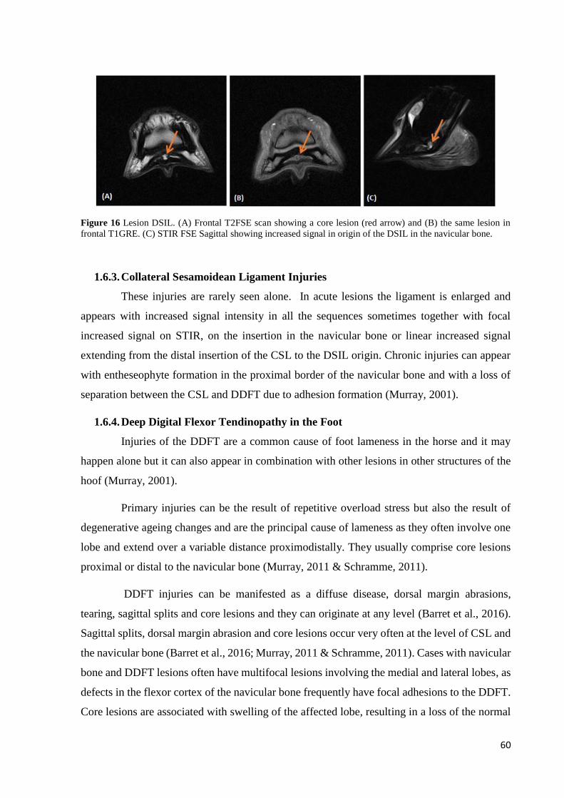
60
Figure 16 Lesion DSIL. (A) Frontal T2FSE scan showing a core lesion (red arrow) and (B) the same lesion in
frontal T1GRE. (C) STIR FSE Sagittal showing increased signal in origin of the DSIL in the navicular bone.
1.6.3. Collateral Sesamoidean Ligament Injuries
These injuries are rarely seen alone. In acute lesions the ligament is enlarged and
appears with increased signal intensity in all the sequences sometimes together with focal
increased signal on STIR, on the insertion in the navicular bone or linear increased signal
extending from the distal insertion of the CSL to the DSIL origin. Chronic injuries can appear
with entheseophyte formation in the proximal border of the navicular bone and with a loss of
separation between the CSL and DDFT due to adhesion formation (Murray, 2001).
1.6.4. Deep Digital Flexor Tendinopathy in the Foot
Injuries of the DDFT are a common cause of foot lameness in the horse and it may
happen alone but it can also appear in combination with other lesions in other structures of the
hoof (Murray, 2001).
Primary injuries can be the result of repetitive overload stress but also the result of
degenerative ageing changes and are the principal cause of lameness as they often involve one
lobe and extend over a variable distance proximodistally. They usually comprise core lesions
proximal or distal to the navicular bone (Murray, 2011 & Schramme, 2011).
DDFT injuries can be manifested as a diffuse disease, dorsal margin abrasions,
tearing, sagittal splits and core lesions and they can originate at any level (Barret et al., 2016).
Sagittal splits, dorsal margin abrasion and core lesions occur very often at the level of CSL and
the navicular bone (Barret et al., 2016; Murray, 2011 & Schramme, 2011). Cases with navicular
bone and DDFT lesions often have multifocal lesions involving the medial and lateral lobes, as
defects in the flexor cortex of the navicular bone frequently have focal adhesions to the DDFT.
Core lesions are associated with swelling of the affected lobe, resulting in a loss of the normal

61
mediolateral symmetry. (Murray, 2011) Possible risk factors for DDFT injuries include hoof
conformation and the angle of the DDFT as it passes over the navicular bone, the horse’s athletic
discipline as it appears that the risk increases with the height and intensity of jumping, previous
palmar digital neurectomy and the presence of navicular bone disease. Horses with palmar
nerve neurectomy have increased risk of progression and deterioration of existing DDFT
lesions, because of continued overloading of the compromised but desensitized DDFT
following surgical procedure (Schramme, 2011). Caution is warranted in horses with navicular
problems and even more in cases with flexor surface erosive lesions as they are often
accompanied by DDFT damage. Neurectomy in these cases can lead to further DDFT damage
or even a rupture and for that reason is contraindicated (Barret et al., 2016). Although dorsal
abrasion lesions on the DDFT are commonly diagnosed in association with navicular bone
disease, more exactly with degenerative changes in the flexor surface of the navicular bone, the
correlation between sagittal splits and core lesion on the DDFT with navicular disease is still
unclear (Murray, 2001).
Figure 17 Lesion DDFT. (A) T1GRE transverse showing a DDFT core-lesion distal to the navicular bone, before
the distal insertion on P3; (B) Transverse T1GRE with DDFT splits in both medial and lateral lobe, at the level of
the navicular bone; (C) T1GRE HR Transverse showing a big core lesion on the lateral lobe of the DDFT with
adhesions to the navicular bursa.
1.6.5. Distal Interphalangeal Joint (DIP)
MRI has provided a noninvasive way to assess the joint and evaluation of the
cartilage, subchondral bone and intra and extra-articular soft tissues as the joint capsule and
collateral ligaments (Barret et al, 2016).
Distention or effusion of the DIP with or without soft tissue proliferation, is a very
common but non-specific finding in many lame horses and does not necessarily reflect primary
joint disease (Murray, 2001). The articular cartilage is more difficult to evaluate in low-field

62
systems due to the inferior resolution. Normally it is associated with focal decreased signal in
T1 sequences or cartilage surface irregularity. If there is an excessive cartilage loss the joint
space will be thinner but variation within the joint space should be evaluated with extreme care
because it can be influenced by the way the horse is standing and the position of the limb in the
magnet (Murray, 2001). This can be accompanied by irregularities in the adjacent subchondral
bone, or increased signal in STIR images (Murray, 2001).
Figure 18 Lesion DIP Joint. (A) T1GRE HR Frontal showing thinning of the cartilage od the DIP joint in the
medial aspect (red circle); (B) T1 GRE 3D Sagittal showing a presence of a fragment (red arrow); (C) Osteophyte
formation in the dorsal aspect of P2.
1.6.6. Collateral Ligaments of DIP Joint
Acute injuries of a CL of the DIP joint is characterised by increased signal
intensity in all images sequences often with swelling and in association with DIP joint effusion.
Transverse images are the most sensitive in the detection of lesions but frontal images can also
be useful (Murray, 2001).
The lesions may be restricted to one portion of the ligament or extend throughout
is entire length. The medial CL is more frequently injured however, both ligaments maybe
injured (Murray, 2011). The lesions are often accompanied by endosteal or periosteal reaction,
i.e. subchondral bone reaction or entheseophyte formation at their origin (P2) or distal insertion
(P3) (Murray, 2001).
T2 FSE and STIR sequences are preferable as the lateral CL is susceptible to magic
angle artifact, resulting in an increased signal intensity in T1 and T2 GR and PD sequences.
Confirmation of a lesion requires a presence of swelling of the ligament and/or periligamentar
tissues, increased signal in T2 FSE and STIR sequences or complete disruption of the ligament
architecture reflecting partial rupture or associated osseous changes (Murray, 2001).

63
1.6.7. Middle and Distal Phalanges
The most common lesions include bone trauma, osseous cyst-like lesions
(OCLL), fractures and axial defects in the palmar process of P3. Bone trauma appears as focal
or diffuse reduced signal intensity in T1- and T2-W and increased signal intensity in STIR
images. The distal dorsal aspect of the middle phalanx is a common site for such lesions but not
necessarily involving other soft tissues. Mild and diffused decreased signal intensity in T1- and
T2-W images in the middle palmar process of P3 has been a common finding but appears to be
clinically irrelevant (Murray, 2001). OCLL normally occur in the subchondral bone on either
P2 or P3 and usually have high signal intensity in STIR. Fractures tend to appear as a linear
increased signal intensity in STIR with reduced signal intensity in T1- and T2-W adjacent to
the fractures (Murray, 2001).
Figure 20 MRI findings in the middle and distal phalax. From the left to the right: First picture, a STIR GRE
Frontal scan, showing a cyst in the pedal bone (red arrow); Sedond picture, a STIR FSE Sagittal, showing dorsal
P2 Bone edema (blue arrow); Third picture, a T1 GRE Frontal 3D, showing a cyst like lesion in the distal aspect
of P1 with connection to the pastern joint (orange arrow); Fourth picture, a T1 GRE Frontal HR, showing a pedal
bone wing reaction (green arrow).
Figure 19 Lesion collateral ligaments of the DIP joint (A) T1 GRE Transverse; (B) T2 FSE PSAT
Transverse; (C) PDW FSE Transverse. Note the increased size of the ligament (Red arrows) and increased
signal in both T2 FSE and PDW FSE showing the presence of inflammation. (D) T” FSE Frontal also
showing swelling and increased signal.

64
III- LOW-FIELD MRI IN PODOTROCHLEOSIS: CASELOAD
1. Material and Methods
The 95 horses in this study were brought as referral cases or examined as first opinion
in the clinic, between September 2015 and September 2016. Signalment included age and
breed. Follow-up examinations were conducted at least 2 months after the initial examination.
The horses selected for this study presented with an acute or chronic forelimb
lameness, uni- or bilateral and showed positive response to either digital palmar nerve or abaxial
sesamoidean anesthesia. The result of clinical and other imaging techniques were inconclusive
and did not explain the cause of lameness. Horses selected in this study had no evidence of
other forelimb pathology elsewere. Both feet or just one were examined on the MRI, depending
if the horse was bilateral or unilateral lame. Lesions in the navicular bone were divided
depending affected area as following: proximal border, spongiosa or dorsal surface, distal
border and flexor surface. The lesions were defined only by presence or absence and not by
their nature and severity.
The MR images were acquired by using a 0,27T Hallmarq. Pulse sequences were
obtained in three planes. Sequences used included T1 3D GRE, T1 SE, STIR FSE, T1 GRE HR
and T2 FSE. In some cases some extra scans were included like T2 GRE, STIR GRE and PDW
SE. Transverse images were orientated perpendicular to the flexor surface, sagittal pictures
were orientated perpendicular to the distal insertion of the DDFT and frontal pictures parallel
to the flexor surface or perpendicular to the distal insertion of the DDFT.
Descriptive statistics were performed on all data to establish the frequency of
occurrence of the lesions in the PTA that included lesions in the navicular bone, navicular bursa,
DSIL, collateral sesamoidean ligaments, DDFT, DIPJ, collateral ligaments of the DIPJ, middle
and distal phalanx. Abnormalities were only recorded if they were repeatable in more than one
plane and in more than one pulse sequence. Artifacts and common anatomic variations were
not classified as abnormalities. A certified veterinarian specialist in diagnostic imaging from
Pferdeklinik Leichlingen analyzed the images from this study and recorded the lesions found.
Statistical correlations between the outcome and variables of treatment were analysed
using a Chi-square test. All analyses were performed with statistical analysis software, SPSS,
with a significance level of 0,05.

65
2. Results
2.1. Case Frequency Analysis: Description of the Sample
As explained before, 95 horses were used in this study: 44 mares, 2 stallions, 46
geldings and 3 were the sex was not recorded.
Figure 21 Sex distribution in the sample.
67,4% of the horses were presented with unilateral lameness and therefore underwent
only unilateral MR examination. The other 32,6% of the horses presented with bilateral
lameness and were subjected to MR examination of both front feet.
Figure 22 Distribution of the lameness: Unilateral vs. Bilateral
This study comtemplated 95 sport horses, with the highest number of cases from the
breed Hannoveraner (16%), followed by Westfalen (14%), Holsteiner (13%) and American
Quarter Horses (12%). The riding disciplines were not recorded.
46%
49%
2% 3%
Mare
Gelding
Stallion
Unknown
67%
33%
1 Limb
2 Limbs

66
Figure 23 Breed distribution in the sample
2.2. Prevalence of Lesions found on the MRI
All findings that might contributed to a lameness were considered as a lesion, although
some findings might not have been the main cause. Anatomical variations and artifacts were
not taken into consideration.
Navicular bone lesions had a prevalence of 38%, most of them being lesions in the
distal border (14%), followed by lesions on the flexor surface (11%), dorsal surface (8%) and
the proximal border (4,6%). The second most common lesion found were coffin-joint lesions
with a prevalence of 16,4%, followed by DDFT lesions with a prevalence of 15,3% and DSIL
lesions with 8,6%. Lesions with less prevalence were pedal bone (6,7%), navicular bursa
(6,5%), collateral ligaments (5,9%), middle phalanx (2,2%) and CSL pathologies (0,8%).
American Quarter Horse Arabisches Halbblut Arabisches Vollblut
Belgisches Warmblut Connemara Pony Deutsches Reitpferde
Deutsches Sportpferde French Warmblood Haflinger
Hannoveraner Zweibrücker Hessisches Warmblut
Holsteiner Unkown Kroatisches Warmblut
KWPN Oldenburger Polnisches Warmblut
Westfale Württemberger Rheinländer
Trakehner
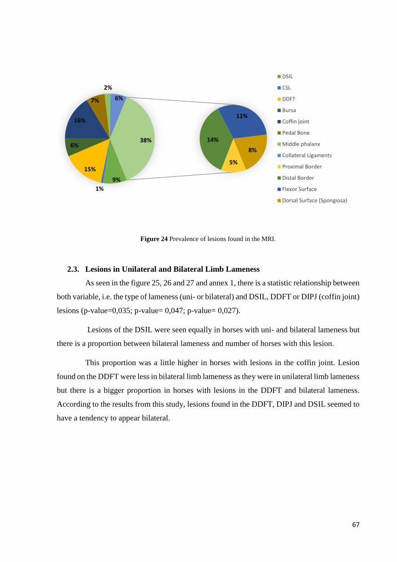
67
Figure 24 Prevalence of lesions found in the MRI.
2.3. Lesions in Unilateral and Bilateral Limb Lameness
As seen in the figure 25, 26 and 27 and annex 1, there is a statistic relationship between
both variable, i.e. the type of lameness (uni- or bilateral) and DSIL, DDFT or DIPJ (coffin joint)
lesions (p-value=0,035; p-value= 0,047; p-value= 0,027).
Lesions of the DSIL were seen equally in horses with uni- and bilateral lameness but
there is a proportion between bilateral lameness and number of horses with this lesion.
This proportion was a little higher in horses with lesions in the coffin joint. Lesion
found on the DDFT were less in bilateral limb lameness as they were in unilateral limb lameness
but there is a bigger proportion in horses with lesions in the DDFT and bilateral lameness.
According to the results from this study, lesions found in the DDFT, DIPJ and DSIL seemed to
have a tendency to appear bilateral.
9%
1%
15%
6%
16%
7%
2%
6%
5%
14%
11%
8%
38%
DSIL
CSL
DDFT
Bursa
Coffin joint
Pedal Bone
Middle phalanx
Collateral Ligaments
Proximal Border
Distal Border
Flexor Surface
Dorsal Surface (Spongiosa)

68
Figure 25 DSIL lesions in unilateral and bilateral lameness. Findings DSIL 0: Absent 1: Present. N__Membro 1:
Unilateral lameness 2: Bilateral lameness
Figure 26 DDFT lesions in unilateral and bilateral lameness. Findings DDFT (TBS) 0: Absent 1: Present.
N__Membro 1: Unilateral lameness 2: Bilateral lameness
Figure 27 Coffin-joint lesions in unilateral and bilateral lameness. Findings Coffin-Joint 0: Absent 1: Present.
N__Membro 1: Unilateral lameness 2: Bilateral lameness

69
2.4. Association of Lesions
It was studied the hypothesis of association between lesions found on the MRI of
horses with frontlimb lameness localized in the foot. Between all lesions found in the horses
that underwent a MRI study, it several relevant statistical relationships were seen.
The strongest statistical relationship was found between lesions in the different areas
in the navicular bone, i.e. proximal border, dorsal surface, distal border and flexor surface. The
association between the presence of lesions in the dorsal and flexor surface had the strongest
statistical relationship among them all (p-value<0,001; phi-coefficient: 0,729) followed by
association of lesions in the proximal border and dorsal surface ( p-value<0,01 , phi-coefficient:
0,704). The association between the presence of lesions in the proximal and distal border had
the lowest score between all areas of the navicular bone, but still with a strong positive statistical
relationship (p-value<0,001; phi-coefficient: 0,434). The results suggest that normally there is
not a singular area affected in the navicular bone but a more diffuse disease should be expected,
maybe the reflect of a rapid evolution. The exact results can be observed in table 8.
Variables Crossed Chi-square Phi
Findings_DorsalSurfaceSpongiosa * Findings_FlexorSurface p<0,001 0,729
Findings_ProximalBorder * Findings_DorsalSurfaceSpongiosa p<0,001 0,704
Findings_DistalBorder * Findings_DorsalSurfaceSpongiosa p<0,001 0,570
Findings_DistalBorder * Findings_FlexorSurface p<0,001 0,548
Findings_ProximalBorder * Findings_FlexorSurface p<0,001 0,513
Findings_ProximalBorder * Findings_DistalBorder p<0,001 0,434 Table 8 Statistical relationships found in the variables of the areas of the navicular bone.
Approximately 38% of the horses in this study did not present any lesion in the
navicular bone at all. As seen in the graphic bellow, no horse presented lesions in the proximal
border and dorsal surface without association to other areas of the navicular bone. 18% of the
horses presented with diffuse lesions, affecting all four different areas. 12% of the horses
presented lesions affecting the distal border, dorsal and flexor surface. 9% of the horses
presented lesions affecting the distal border and the flexor surface and a minority of 1% with
lesions affecting the flexor and dorsal surface.
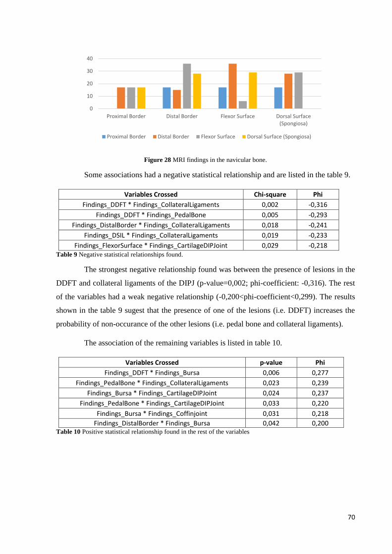
70
Figure 28 MRI findings in the navicular bone.
Some associations had a negative statistical relationship and are listed in the table 9.
Variables Crossed Chi-square Phi
Findings_DDFT * Findings_CollateralLigaments 0,002 -0,316
Findings_DDFT * Findings_PedalBone 0,005 -0,293
Findings_DistalBorder * Findings_CollateralLigaments 0,018 -0,241
Findings_DSIL * Findings_CollateralLigaments 0,019 -0,233
Findings_FlexorSurface * Findings_CartilageDIPJoint 0,029 -0,218 Table 9 Negative statistical relationships found.
The strongest negative relationship found was between the presence of lesions in the
DDFT and collateral ligaments of the DIPJ (p-value=0,002; phi-coefficient: -0,316). The rest
of the variables had a weak negative relationship (-0,200<phi-coefficient<0,299). The results
shown in the table 9 sugest that the presence of one of the lesions (i.e. DDFT) increases the
probability of non-occurance of the other lesions (i.e. pedal bone and collateral ligaments).
The association of the remaining variables is listed in table 10.
Variables Crossed p-value Phi
Findings_DDFT * Findings_Bursa 0,006 0,277
Findings_PedalBone * Findings_CollateralLigaments 0,023 0,239
Findings_Bursa * Findings_CartilageDIPJoint 0,024 0,237
Findings_PedalBone * Findings_CartilageDIPJoint 0,033 0,220
Findings_Bursa * Findings_Coffinjoint 0,031 0,218
Findings_DistalBorder * Findings_Bursa 0,042 0,200 Table 10 Positive statistical relationship found in the rest of the variables
0
10
20
30
40
Proximal Border Distal Border Flexor Surface Dorsal Surface(Spongiosa)
Proximal Border Distal Border Flexor Surface Dorsal Surface (Spongiosa)

71
3. Discussion
The main objective of this study was to investigate the prevalence of lesions associated
with the PTA in sport horses that underwent an MRI examination of the front feet. The second
aim was to investigate which lesions do commonly appear together.
The results support that pain localised to the foot may be associated with MR changes
in a variety of structures, and that lesions to several structures may occur concurrently, probably
due to the closed anatomical relationship between some of the structures (Dyson & Murray,
2007; Murray et al., 2006).
Abnormalities in the navicular bone (40%), DIPJ (16%), DDFT (15%) and DSIL (9%)
predominated in the investigated population. Concurrent lesions in the navicular bone, DDFT
and DSIL are already well documented (Wright et al., 1998).
In the investigated population, lesions or alterations in the DIPJ were usually not
associated with any other concurrent pathology of a adjacent structures. This suggests that it
seems to occur mostly as a separate disease process from the other structures supported by R.M
in 2006 (Murray et al., 2006). Other studies suggest that the close anatomical relationship
between the DIPJ and the navicular bone can potentially lead to an association of lesions (Dyson
& Murray, 2007) and to other microinjuries of the DSIL and DDFT (Kimberly et al., 1997).
This is caused by major-weight bearing pressures and dorsiflexion movements during normal
locomotion (Dyson & Murray, 2007). The mechanical loading triggers a cascade of molecular
events that may lead to disease in susceptible individuals by increasing the production and
release of free radicals, cytokines, fatty acid catabolites, neuropeptides and matrix-degrading
enzymes. These molecules may be involved in the remodeling of articular and subchondral
bone structures. If the adaptive capacity of a joint is exhausted, an increase in biomarkers may
be detectable (Rijkenhuisen, 2006). Changes in biochemical markers in the DIPJ and navicular
bursa have been observed in horses with clinical “navicular disease”. The increase of
biochemical markers are an expression of an active inflammatory process, but in chronic cases
they do not always reflect the damage accumulated over a long time period (Rijkenhuisen,
2006). Therefore their reliability for indicating pathology in any given joint has not been
confirmed yet (McIlwraith, 2005).
In this study, pathologic findings in the cartilage of the DIPJ had a positive statistical
relationship with findings in the pedal bone, reflecting the extension of the lesions to the
subchondral area. There was also a positive statistical relationship between cartilage defects of

72
the DIPJ and navicular bursa pathology. Concurrent lesions of the dorsal surface of the
navicular bone and DIPJ pathology were seen in several horses, but no statistical relationship
was found.
Findings in the DSIL had no statistical relationship to findings in the DDFT, navicular
bone, CSL or navicular bursa as it was described in previous studies (Dyson & Murray, 2007;
Murray et al., 2006). Findings of the DSIL had a negative statistical relationship with findings
of the collateral ligaments of the DIPJ, not supporting preview studies (Dyson et al., 2011).
This could be related to the population of horses which were included in this study.
Findings in the DDFT were a common feature. There was a positive statistical
relationship between findings on the DDFT and findings in the navicular bursa. Association of
DDFT lesions with pedal bone and collateral ligament injuries of the DIPJ had a negative
statistical relationship. In previews studies, there was found an association of lesions between
the DDFT and DSIL and/or CSL (Dyson & Murray, 2007), but this was not observed in the
horses in this study. Association of lesions between the DDFT and the navicular bursa can be
expected due to the close anatomy, particularly in cases with lesions of the dorsal surface of the
DDFT and navicular bursitis (Schramme, 2011). Lesions of the DDFT are more often seen at
the level of the CSL and navicular bone followed by the level of the DSIL and distal insertion
(Dyson & Murray, 2007). This study suggest that the increase of and DDFT injuries potentially
decreases the possibility of bone injuries at the level of the palmar process of the pedal bone
and the likelihood of collateral ligaments of the DIPJ pathology. Although when looking at the
biomechanical closed relationship of these two structures one would expect otherwise. This
also could be a result of case selection.
There was a positive association between lesions of the navicular bursa and distal
border lesions of the navicular bone as described previously in other studies (Dyson et al., 2003;
Dyson and Murray, 2007).
There was also a positive association between lesions in the collateral ligaments of the
DIPJ and lesions of the pedal bone. It has been suggested that lateromedial or rotational motion
of the DIPJ may result in damage to the collateral ligaments that might occur within the body
of the ligament or at the attachments of the ligament to the pedal bone (Zubrod et al., 2005).
Thought in this study, no relationship was found between lesions of the collateral ligaments and
coffin joint pathology (annex 4), the same results were observed in an other study (Murray et
al., 2006).

73
There was a negative statistical relationship in the association of lesions between the
collateral ligaments of the DIPJ and the distal border of the navicular bone and DDFT, not yet
supported by other studies.
Some of the associations already described in previous studies didn’t had a significant
statistic relashionship in the horses from this study. This and other not explainable
relashionships found in the sample or any association not described in the consulted references
might be a result of some limitiations. The limitations included the fact that horses with
unilateral limb lameness were only subjected to an unilateral MRI examination due to the costs
of the examination but decreasing the study rigorousness. Another limitation was that the
inclusion criteria of the horses in this study included the lack of findings in clinical examination
and other imaging diagnostic tecniques. This may lead to a loss of findings of expected
associations, since horses with lesions diagnosed by radiology were automatically non selected.

74
4. Conclusion
Palmar foot pain is a common cause of lameness in the horse and can be the result of
several clinical conditions. Results of this study support that several combinations of problems
might contribute to the lameness seen in affected horses.
The wide variety of possible injured tissues within the hoof makes it challanging to
the clinicians to define the exact diagnosis. It is essential to a obtain a detailed history and to
perform an accurate lameness investigation prior to the MR examination. Diagnostic anesthesia
should always be performed (except cases with suspected hairline fractures) to assure that the
hoof is the primary source of pain. Other diagnostic imaging modalities like radiology and
ultrasonography should also be performed prior to MR exam, to exclude or confirm differential
diagnoses, when possible.
MR examinations are expensive and for this reason should only be carried out when
other imaging techniques fail to achieve a final diagnosis, or when further information about
the nature of the lesions and distribution is necessary. MRI is a useful tool not only in providing
a specific diagnosis in cases that were previously grouped into the vague diagnosis of palmar
heel pain, but also in providing a more accurate prognosis and a more targeted treatment and
rehabilitation.
The amount of possible lesions and associations of lesions found in this study, were
quite extensive, which makes a more structured categorization of possible lesion associations
almost impossible. For this reason, every case should always be evaluated as a individual
situation.
The increasing knowledge of underlying molecular biologic processes, anatomy,
possible pathologies and their response to medical or surgical treatment and rehabilitation helps
in conceiving possible outcomes and evolution of the pathology itself.
Navicular bone pathologies continue to be a major cause of frontlimb lameness, but
concurrent or associated injuriess of other related structures such as the DDFT, DSIL or DIPJ
should always be considered due to their close anatomical relationship.
75
References
Armstrong, P. & Stephen, F.K. (1991) Magnetic Resonance imaging-1: basic principles of
image production. BMJ 303, 35-40.
Auer; J. & Stick, J. (1999) Equine Surgery (2nd Ed., pp. 611-619). USA
Barret, M.F., Frisbie, D.D., King, M.R., Werpy, N.M. & Kawcak, C.E. (2016) A review of how
magnetic resonance imaging can aid in case management of common pathological conditions
of the equine foot. Equine Veterinay Education, doi: 10.1111/eve.12542.
Busoni, V. & Denoix, J.-M. (2001) Ultrasonography of the podotrochlear apparatus in the horse
using a transcuneal approach: Technique and reference images. Veterinary Radiology and
Ultrasound, 42 (6), 534-540.
Butler, J., Colles, C., Dyson, S., Kold, S. & Poulos, P. (2000) Clinical Radiology of the Horse
(2ndEd) (pp. 27-83)
Dabareiner, R., Carter, G. & Honnas, C. (2001) How to Perform Navicular Bursa Injection and
Indications for its Use. Proceedings of the Annual Convention of the AAEP.
Damadian, R. (1971) Tumor Detection by Nuclear Magnetic Resonance. Science, 171, 1151-
1153.
Damadian, R., Zaner, K. Hor, D., DiMaio, T. (1974) Human Tumors Detected by Nuclear
Magnetic Resonance. PNAS USA, 71 (4), 1471-1473.
Damadian, R., Minkoff, L., Goldsmith, M., Stanford, M. Koutcher, J. (1976) Field focusing
Nuclear Magnetic Resonance (FONAR): Visualization of a Tumor in a Live Animal. Science,
Vol. 194, 1430-1432.
Dyson, S. & Murray, R. (2007) Magnetic resonance imaging evaluation of 264 horses with foot
pain: the podotrochlear apparatus, deep digital flexor tendon and collateral ligaments of the
distal interphalangeal joint. Equine Veterinary Journal. 39(4), 340-3.
Dyson, S., Murray, R., Schramme, M. & Blunden, T. (2011) Current concepts of navicular
disease. Equine Veterinary Education, 23 (1), 27-39.
Dyson, S., Murray, R., Schramme, M. & Branch, M. (2003) Magnetic resonance imaging of
the equine foot: 15 horses. Equine Veterinary Journal, 35 (1), 18-26.

76
Hallmarq Veterinay Imaging (2007) MRI Artifacts- and how to avoid them. Surrey, UK
Hallmarq Veterinay Imaging (2011) The Hallmarq MRI sequence library. Surrey, UK
Hartwig, V., Giovannetti, G., Vanello, N., Lombardi, M., Landini, L. & Simi, S. (2009)
Biological Effects and Safety in Magnetic Resonance Imaging: A Review. Int. J. Environ. Res.
Public Health, 6(6), 1778-1798.
Hinchcliff, K., Kaneps, A. & Geor, R. (2004) Equine Sports Medicine and Surgery. London,
UK.
Jacquet, S. & Denoix, J.-M. (2012) Ultrasonographic examination of the distal podotrochlear
apparatus of the horse: A transcuneal approach. Equine Veterinary Education, 24 (2), 90-96.
Kimberly K., Van Wulfen, B.S. & Bowker, R.M. (1997) Intersection of the DSIL and the DDFT
and Its Relationship to Navicular Syndrome. Proceedings of the 43rd AAEP Annual
Convention. Phoenix, Arizona. USA.
Kleiter, M.; Kneissl, S.; Stanek, C.; Mayrhofer, E.; Baulain, U. & Deegen, E. (1999) Evaluation
of magnetic resonance imaging techniques in the equine digit. Vet. Radiol. Ultrasound. 40, 15-
22.
Kristoffersen, M. & Thoefner, M.B. (2003) Ultrasonography of the navicular region in horses.
Equine Veterinary Education, 15 (3), 150-157.
Labruyère, J., Schwarz, T. (2013) CT and MRI in veterinary patients: an update on recent
advances. In Practice BMJ Journals, 35 (10) 546-563.
Lauterbur PC. (1973) Image formation by induced local interations: examples employing
nuclear magnetic resonance. Nature 1973; 242:190.
Magnetic Resonance- Technology Information Portal (2003). Acess in 3rd December 2017 in
www.mr-tip.com
Mair, T.S., Kinns, J., Jones, R.D. & Bolas, N.M. (2005) Magnetic resonance imaging of the
distal limb of the standing horse. Equine Veterinary Education, 17 (2), 74-78.
Martinelli, M. & Rantanen, N. (2002) The Role of Select Imaging Studies in the Lameness
Examination. Proceedings of the Annual Convention of the AAEP.

77
McIlwraith, C.W. (2005) Use of synovial fluid and serum biomarkers in equine bone and joint
disease: a review. Equine Veterinary Journal. 37 (5), 473-482.
Moyer, W. (2010) Practical Aspects of Diagnosing Lameness in Horses: A Suggested
Procedure for Performing the Physical and Motion Examination. AAEP.
Murray, R. (2001) Equine MRI. Newmarket, UK.
Murray, R.; Schramme, M.; Dyson, S.; Branch, M. & Blunden, T. (2006) Magnetic Resonance
Imaging Characteristics of the Foot in Horses with Palmar Foot Pain and Control Horses. Vet
Radiology & Ultrasound. 47 (1), 1-16.
Rijkenhuisen, A. (2006) Navicular disease: a review of what’s new. Equine Veterinary Journal,
38(1), 82-88.
Ross, M. & Dyson, S. (2003). Diagnosis and management of lameness in the horse. St. Louis,
Missouri, USA.
Schneider, R.K. (2007) Impar ligament injury can cause lameness in performance horses.
Equine Veterinary Education, 19 (3) , 121-122.
Schramme, M.C. (2011) Deep digital flexor tendonopathy in the foot. Equine Veterinary
Education, 23(8), 403-415.
Schramme, M., Schumacher, J. & Schumacher J. (2007) Clinical Examination, Differential
Analgesia and Imaging Modalities for Investigation of Distal Limb Lameness. American
Association of Equine Practitioners- AAEP- Fort Collins, Colorado, USA.
Schramme, M., Schumacher, J. & Schumacher J. (2015) Diagnostic Analgesia of the Foot:
Techniques & Interpretation. Proceeding of the Belgian Equine Practitioners Society. Leuven,
Belgium.
Waguespack, W. & Hanson, R. (2010) Navicular Syndrome in Equine Patients: Anatomy,
Causes and Diagnosis. Auburn University. ACVS.
Werner, H. (2013) How to perform basic nerve blocks in the field. 13th WEVA Congress.
Budapest, Hungary.
Widmer, W & Fessler, J. (2002) Review: Understanding Radiographic Changes Associated
with Navicular Syndrome- Are We Making Progress? Proceedings of the Annual Convention
of the AAEP.
78
Wright, I., Kidd, L. & Thorp, B. (1998) Gross, histological and histomorphometric features of
the navicular bone and related structures in the horse. Equine Veterinary Journal. 30 (3), 220-
234.
Zubrod, C., Farnsworth, K. Tucker, R. & Ragle, C. (2005) Injury of the collateral ligaments of
the distal interphalangeal joint diagnosed by magnetic resonance. Veterinary Radiology &
Ultrasound. 46 (1), 11-16.
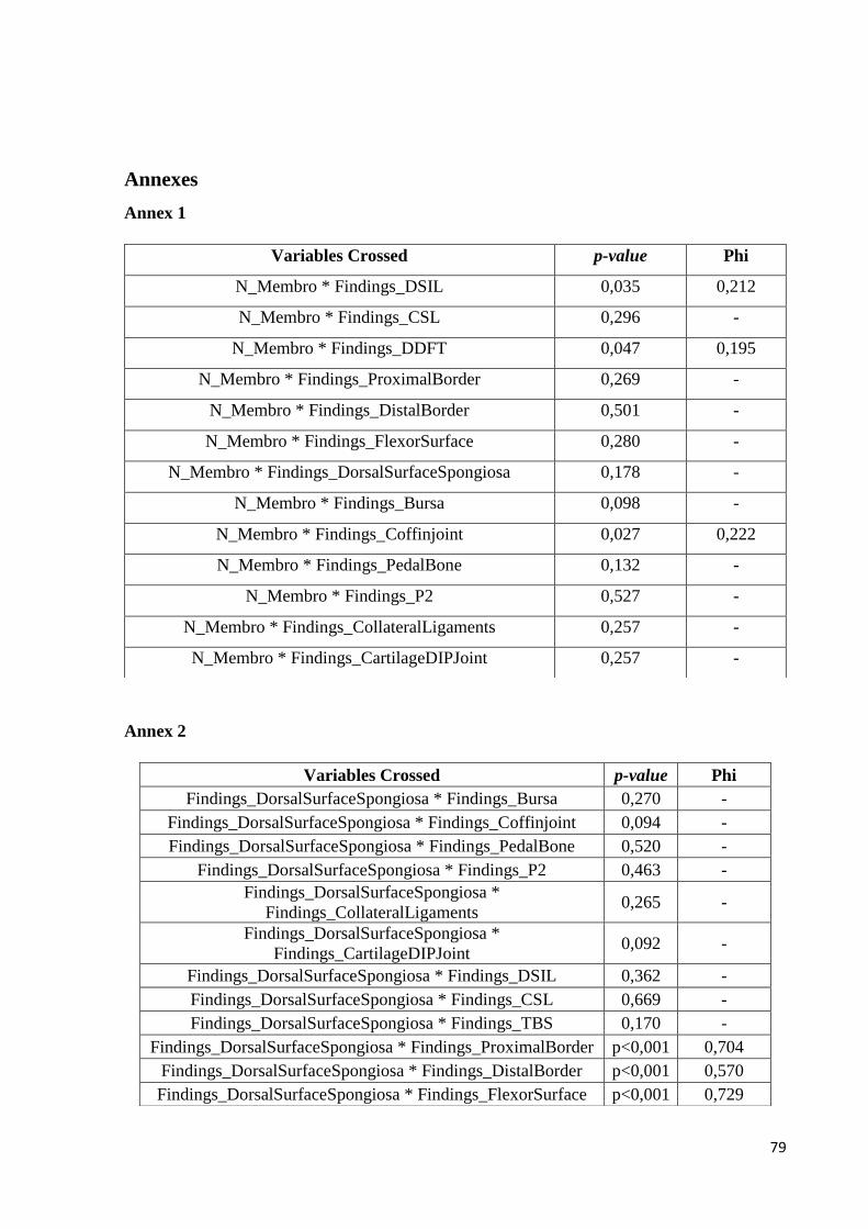
79
Annexes
Annex 1
Annex 2
Variables Crossed p-value Phi
N_Membro * Findings_DSIL 0,035 0,212
N_Membro * Findings_CSL 0,296 -
N_Membro * Findings_DDFT 0,047 0,195
N_Membro * Findings_ProximalBorder 0,269 -
N_Membro * Findings_DistalBorder 0,501 -
N_Membro * Findings_FlexorSurface 0,280 -
N_Membro * Findings_DorsalSurfaceSpongiosa 0,178 -
N_Membro * Findings_Bursa 0,098 -
N_Membro * Findings_Coffinjoint 0,027 0,222
N_Membro * Findings_PedalBone 0,132 -
N_Membro * Findings_P2 0,527 -
N_Membro * Findings_CollateralLigaments 0,257 -
N_Membro * Findings_CartilageDIPJoint 0,257 -
Variables Crossed p-value Phi
Findings_DorsalSurfaceSpongiosa * Findings_Bursa 0,270 -
Findings_DorsalSurfaceSpongiosa * Findings_Coffinjoint 0,094 -
Findings_DorsalSurfaceSpongiosa * Findings_PedalBone 0,520 -
Findings_DorsalSurfaceSpongiosa * Findings_P2 0,463 -
Findings_DorsalSurfaceSpongiosa *
Findings_CollateralLigaments 0,265 -
Findings_DorsalSurfaceSpongiosa *
Findings_CartilageDIPJoint 0,092 -
Findings_DorsalSurfaceSpongiosa * Findings_DSIL 0,362 -
Findings_DorsalSurfaceSpongiosa * Findings_CSL 0,669 -
Findings_DorsalSurfaceSpongiosa * Findings_TBS 0,170 -
Findings_DorsalSurfaceSpongiosa * Findings_ProximalBorder p<0,001 0,704
Findings_DorsalSurfaceSpongiosa * Findings_DistalBorder p<0,001 0,570
Findings_DorsalSurfaceSpongiosa * Findings_FlexorSurface p<0,001 0,729
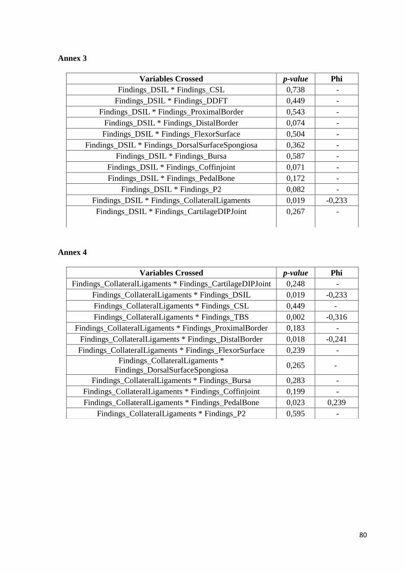
80
Annex 3
Annex 4
Variables Crossed p-value Phi
Findings_DSIL * Findings_CSL 0,738 -
Findings_DSIL * Findings_DDFT 0,449 -
Findings_DSIL * Findings_ProximalBorder 0,543 -
Findings_DSIL * Findings_DistalBorder 0,074 -
Findings_DSIL * Findings_FlexorSurface 0,504 -
Findings_DSIL * Findings_DorsalSurfaceSpongiosa 0,362 -
Findings_DSIL * Findings_Bursa 0,587 -
Findings_DSIL * Findings_Coffinjoint 0,071 -
Findings_DSIL * Findings_PedalBone 0,172 -
Findings_DSIL * Findings_P2 0,082 -
Findings_DSIL * Findings_CollateralLigaments 0,019 -0,233
Findings_DSIL * Findings_CartilageDIPJoint 0,267 -
Variables Crossed p-value Phi
Findings_CollateralLigaments * Findings_CartilageDIPJoint 0,248 -
Findings_CollateralLigaments * Findings_DSIL 0,019 -0,233
Findings_CollateralLigaments * Findings_CSL 0,449 -
Findings_CollateralLigaments * Findings_TBS 0,002 -0,316
Findings_CollateralLigaments * Findings_ProximalBorder 0,183 -
Findings_CollateralLigaments * Findings_DistalBorder 0,018 -0,241
Findings_CollateralLigaments * Findings_FlexorSurface 0,239 -
Findings_CollateralLigaments *
Findings_DorsalSurfaceSpongiosa 0,265 -
Findings_CollateralLigaments * Findings_Bursa 0,283 -
Findings_CollateralLigaments * Findings_Coffinjoint 0,199 -
Findings_CollateralLigaments * Findings_PedalBone 0,023 0,239
Findings_CollateralLigaments * Findings_P2 0,595 -