Low frequency passive seismic interferometry for

land data

Sjoerd de Ridder

ABSTRACT

Here we report results achieved by low-frequency seismic interferometry on a pas-sive seismic land dataset recorded at a field in Saudi Arabia. Computed spectrafor different portions of the data show a time varying ambient seismic wavefielddisplaying a diurnal pattern. At low frequencies (< 10 Hz) the ambient seismicwavefield mainly consists of surface waves in two modes, the fundamental modepropagates with a velocity of about 1250 ms. Results suggest that sufficientcoherent energy is recorded between 1 Hz and 7 Hz for retrieval of a Rayleighsurface wave. The strength of the ambient seismic field affects the convergencerate of the correlations. The directionality in the ambient seismic field affects theradiation pattern of the virtual sources. Retrieved Rayleigh waves at low frequen-cies show spatial variation and dispersive behavior. Dispersion curve estimationopens opportunities for reservoir monitoring by background velocity estimation.

INTRODUCTION

Seismic interferometry aims to retrieve the Green’s function between two receiver sta-tions by correlating measurements of seismic responses at both stations, effectivelyturning one station into a virtual source (Claerbout, 1968; Wapenaar, 2004). Re-cently, a variety of applications have been developed for active seismic data, such asthe virtual source method (Bakulin and Calvert, 2006), redatuming (Schuster et al.,2004; Schuster and Zhou, 2006), and imaging of multiples (Berkhout and Verschuur,2006). Commonly, active seismic (controlled source) interferometry attempts to re-construct the high-frequency (> 10 Hz) impulse response of the earth. Passive seis-mic interferometry has mainly focused on retrieving high-frequency virtual sourceswhere acquiring data with real sources is undesirable. Thus far, results of passiveseismic interferometry have been less than promising, partially due to directionalityof the ambient seismic wavefield and poor sampling of the medium by passive seis-mic sources. Early attempts of Cole (1995), (Artman, 2006, 2007) yielded less thansatisfactory results; more recently, Dragonov et al. (2007) retrieved high-frequencyreflection events from pre-selected body-wave events. Meanwhile, global seismolo-gists have been successful using seismic interferometry to retrieve Green’s functionsat much lower frequency. More recently, the ambient seismic field at lower frequencies(< 10) Hz has been shown to contain sufficient coherent and omnidirectional seismic

SEP–140

de Ridder 2 Low frequency passive SI

energy to yield low-frequency Green’s functions containing direct arrivals in a marineenvironment. Dellinger (2008) pointed out that conventional arrays record useableenergy at low frequencies, while Dellinger and Yu (2009), Landes et al. (2009) andBussat and Kugler (2009) have reported on the use of low-frequency seismic energyrecorded in marine environments to image shallow seafloor structures.

An ambient seismic field recorded above a field in Saudi Arabia has previouslybeen studied using novel imaging methods to locate microseismic events (Fu andLuo, 2009) and seismic interferometery to retrieve high frequency events (Xiao et al.,2009). Here we show interferometric retrieval of the Rayleigh surface waves at lowfrequencies. These surface waves are further studied for potential reservoir monitor-ing and imaging capabilities. Data availability limits the study to a conventionalmicrotremor dispersion-curve analysis technique (Aki, 1957), which assumes later-ally invariant media. However, more generally the retrieved Green’s function can bestudied and imaged without implicit lateral invariant assumptions.

AMBIENT SEISMIC WAVEFIELD

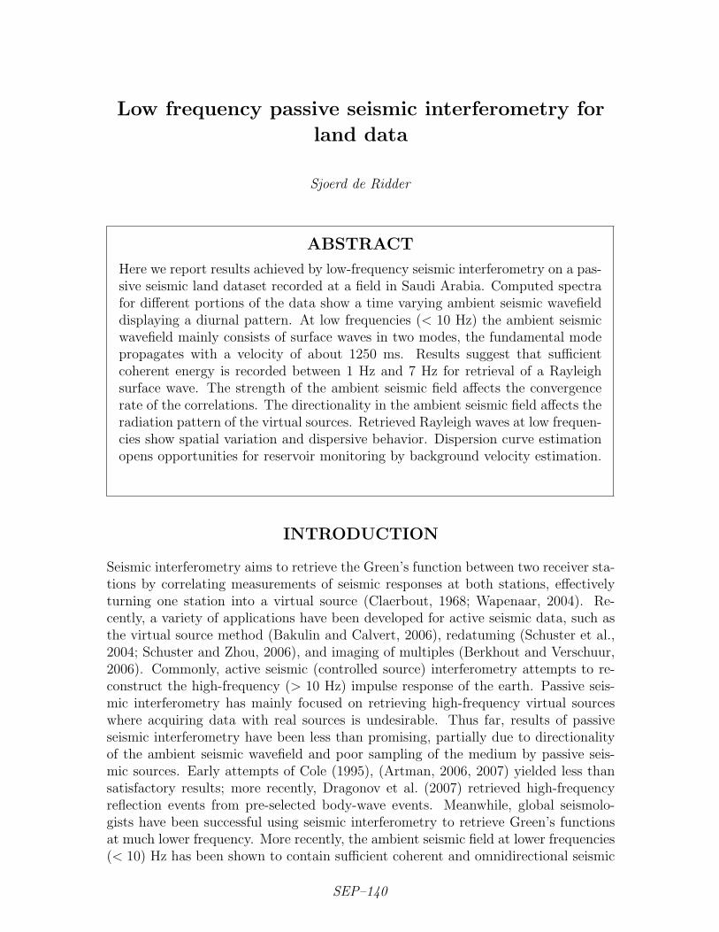
In 2007, Saudi Aramco initiated an experiment aiming to detect and characterizemicroseismic energy for reservoir monitoring (Jervis and Dasgupta, 2009). The surfacearray consisted of 225 buried 3-component stations placed in a 15 by 15 grid withstation spacing of 200 m, spanning an area 3 km by 3 km.

Figure 1: Geometry of theAramco passive experiment; 225stations (denoted by triangles)placed in a 15 by 15 grid. Thegeographic North is indicated byN. Open triangles denote stationsturned into virtual sources for Fig-ures 7 and 8. Lines denote receiverlines for sections shown in Figure7. [NR] gy [

m]0

1000

-1000-1000

0

1000

gx [m]

N

∆y = 200m∆x = 200m

Stanford University received a nearly continuous raw data record spanning 48hours divided over 3 days, starting on day 1 at 18:00 ending on day 3 at 18:00. Onlyvertical components were used, after removing the arithmetic mean over 30 s timewindows. The 48 hours of passive data were analyzed for their spectral characteristics.

SEP–140

de Ridder 3 Low frequency passive SI

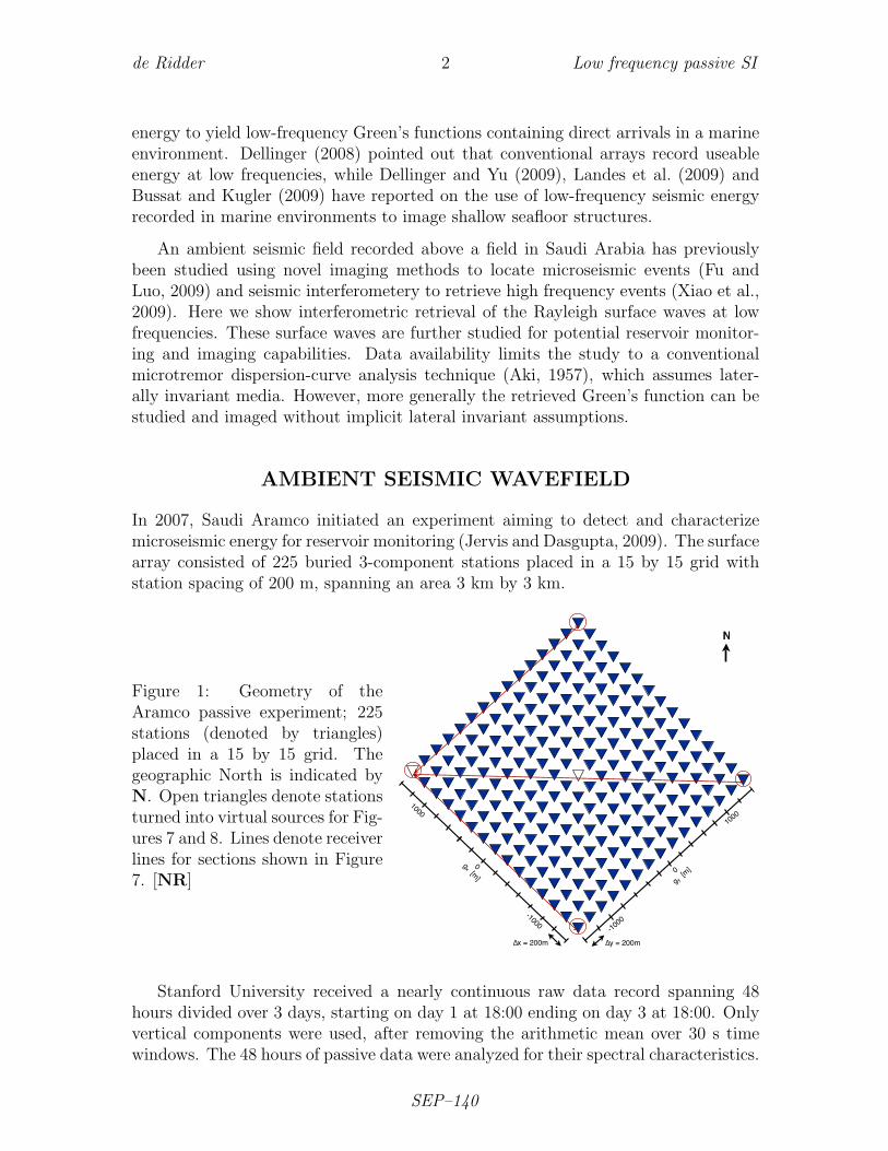
A frequency domain amplitude spectrogram averaged over the entire array is shownin Figure 2. Most energy was recorded between 2 Hz and 12 Hz and varies in a dailypattern with higher energy during the daylight hours and less energy at night. Figure3 shows the frequency-domain amplitude spectrum, averaged for all recordings duringthe hour from 20:00 to 21:00 on day 1, drawn as curve (a). We identify a peak atvery low frequencies, below 1 Hz.

0 20 40 60 80 100f [H

z]

0 4 8 12 16 20f [H

z]

day [#]32

day [#]32

a) b)

Figure 2: Frequency-domain amplitude spectrum averaged over the array as a func-tion of time for 48 hours. White grid lines denote 6 hour blocks. a) Frequency-domainamplitude spectrum between 0 Hz and 100 Hz; b) frequency-domain amplitude spec-trum between 0 Hz and 20 Hz; the black line denotes the frequency of the low-passfilter applied before interferometry. [CR]

amplitude

0 1 2 3 4 5 6 7f [Hz]

abc

Figure 3: Normalized frequency-domain amplitude spectrum, averaged over the ar-ray and data recorded between 20:00 and 21:00 on day 1. Curve (a) is the spectrumof the original data record, curve (c) is the spectrum after low-pass filtering for in-terferometry and curve (b) is the spectrum of the data after band-pass filtering forbeam-forming. [CR]

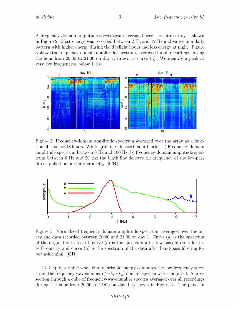
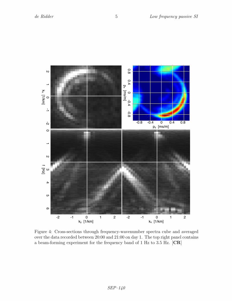
To help determine what kind of seismic energy composes the low-frequency spec-trum, the frequency-wavenumber (f−kx−ky) domain spectra were computed. A crosssection through a cube of frequency-wavenumber spectra averaged over all recordingsduring the hour from 20:00 to 21:00 on day 1 is shown in Figure 4. The panel in

SEP–140

de Ridder 4 Low frequency passive SI

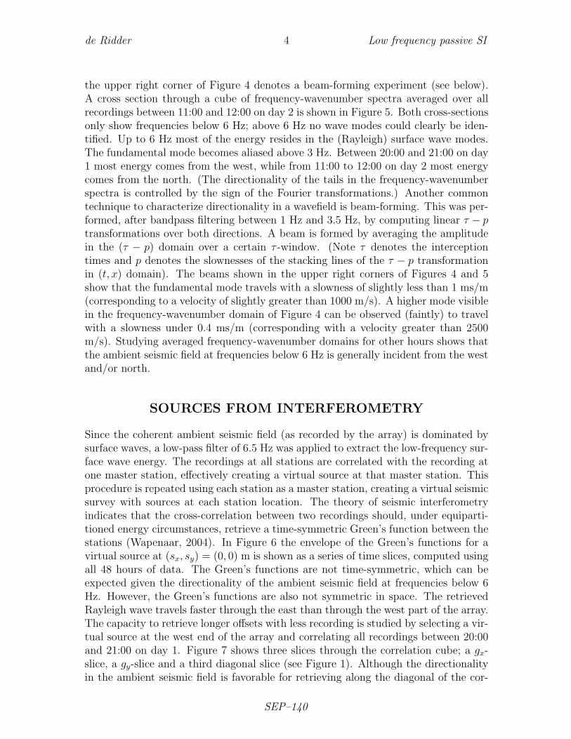
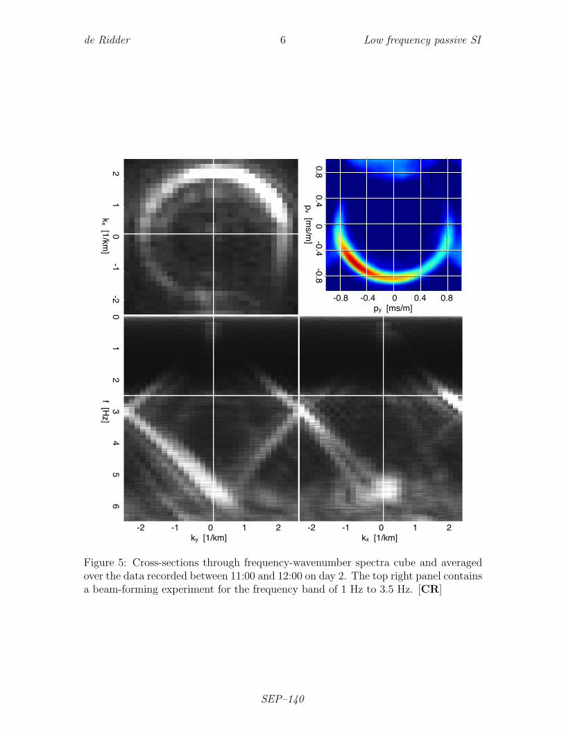
the upper right corner of Figure 4 denotes a beam-forming experiment (see below).A cross section through a cube of frequency-wavenumber spectra averaged over allrecordings between 11:00 and 12:00 on day 2 is shown in Figure 5. Both cross-sectionsonly show frequencies below 6 Hz; above 6 Hz no wave modes could clearly be iden-tified. Up to 6 Hz most of the energy resides in the (Rayleigh) surface wave modes.The fundamental mode becomes aliased above 3 Hz. Between 20:00 and 21:00 on day1 most energy comes from the west, while from 11:00 to 12:00 on day 2 most energycomes from the north. (The directionality of the tails in the frequency-wavenumberspectra is controlled by the sign of the Fourier transformations.) Another commontechnique to characterize directionality in a wavefield is beam-forming. This was per-formed, after bandpass filtering between 1 Hz and 3.5 Hz, by computing linear τ − ptransformations over both directions. A beam is formed by averaging the amplitudein the (τ − p) domain over a certain τ -window. (Note τ denotes the interceptiontimes and p denotes the slownesses of the stacking lines of the τ − p transformationin (t, x) domain). The beams shown in the upper right corners of Figures 4 and 5show that the fundamental mode travels with a slowness of slightly less than 1 ms/m(corresponding to a velocity of slightly greater than 1000 m/s). A higher mode visiblein the frequency-wavenumber domain of Figure 4 can be observed (faintly) to travelwith a slowness under 0.4 ms/m (corresponding with a velocity greater than 2500m/s). Studying averaged frequency-wavenumber domains for other hours shows thatthe ambient seismic field at frequencies below 6 Hz is generally incident from the westand/or north.

SOURCES FROM INTERFEROMETRY

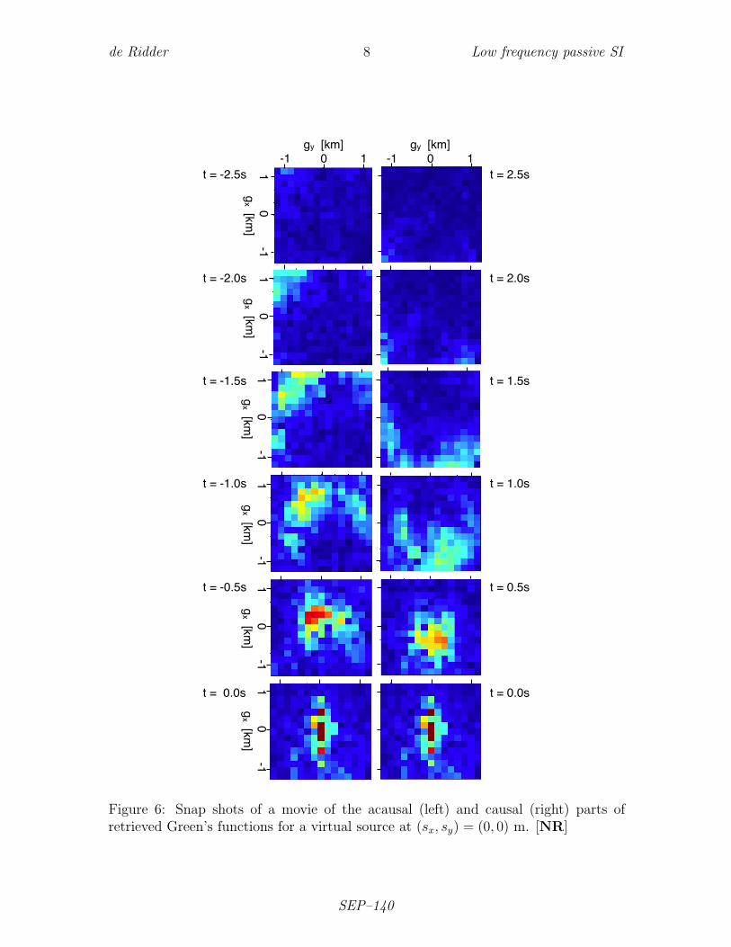
Since the coherent ambient seismic field (as recorded by the array) is dominated bysurface waves, a low-pass filter of 6.5 Hz was applied to extract the low-frequency sur-face wave energy. The recordings at all stations are correlated with the recording atone master station, effectively creating a virtual source at that master station. Thisprocedure is repeated using each station as a master station, creating a virtual seismicsurvey with sources at each station location. The theory of seismic interferometryindicates that the cross-correlation between two recordings should, under equiparti-tioned energy circumstances, retrieve a time-symmetric Green’s function between thestations (Wapenaar, 2004). In Figure 6 the envelope of the Green’s functions for avirtual source at (sx, sy) = (0, 0) m is shown as a series of time slices, computed usingall 48 hours of data. The Green’s functions are not time-symmetric, which can beexpected given the directionality of the ambient seismic field at frequencies below 6Hz. However, the Green’s functions are also not symmetric in space. The retrievedRayleigh wave travels faster through the east than through the west part of the array.The capacity to retrieve longer offsets with less recording is studied by selecting a vir-tual source at the west end of the array and correlating all recordings between 20:00and 21:00 on day 1. Figure 7 shows three slices through the correlation cube; a gx-slice, a gy-slice and a third diagonal slice (see Figure 1). Although the directionalityin the ambient seismic field is favorable for retrieving along the diagonal of the cor-

SEP–140

de Ridder 5 Low frequency passive SI

-0.8 -0.4 0 0.4 0.8py [ms/m]

0.8 0.4 0 -0.4 -0.8px [m

s/m]

0 1 2 3 4 5 6f [H

z] 2 1 0 -1 -2

kx [1/km

]

-2 -1 0 1 2kx [1/km]

-2 -1 0 1 2ky [1/km]

Figure 4: Cross-sections through frequency-wavenumber spectra cube and averagedover the data recorded between 20:00 and 21:00 on day 1. The top right panel containsa beam-forming experiment for the frequency band of 1 Hz to 3.5 Hz. [CR]

SEP–140

de Ridder 6 Low frequency passive SI

-0.8 -0.4 0 0.4 0.8py [ms/m]

0.8 0.4 0 -0.4 -0.8px [m

s/m]

0 1 2 3 4 5 6f [H

z] 2 1 0 -1 -2

kx [1/km

]

-2 -1 0 1 2kx [1/km]

-2 -1 0 1 2ky [1/km]

Figure 5: Cross-sections through frequency-wavenumber spectra cube and averagedover the data recorded between 11:00 and 12:00 on day 2. The top right panel containsa beam-forming experiment for the frequency band of 1 Hz to 3.5 Hz. [CR]

SEP–140

de Ridder 7 Low frequency passive SI

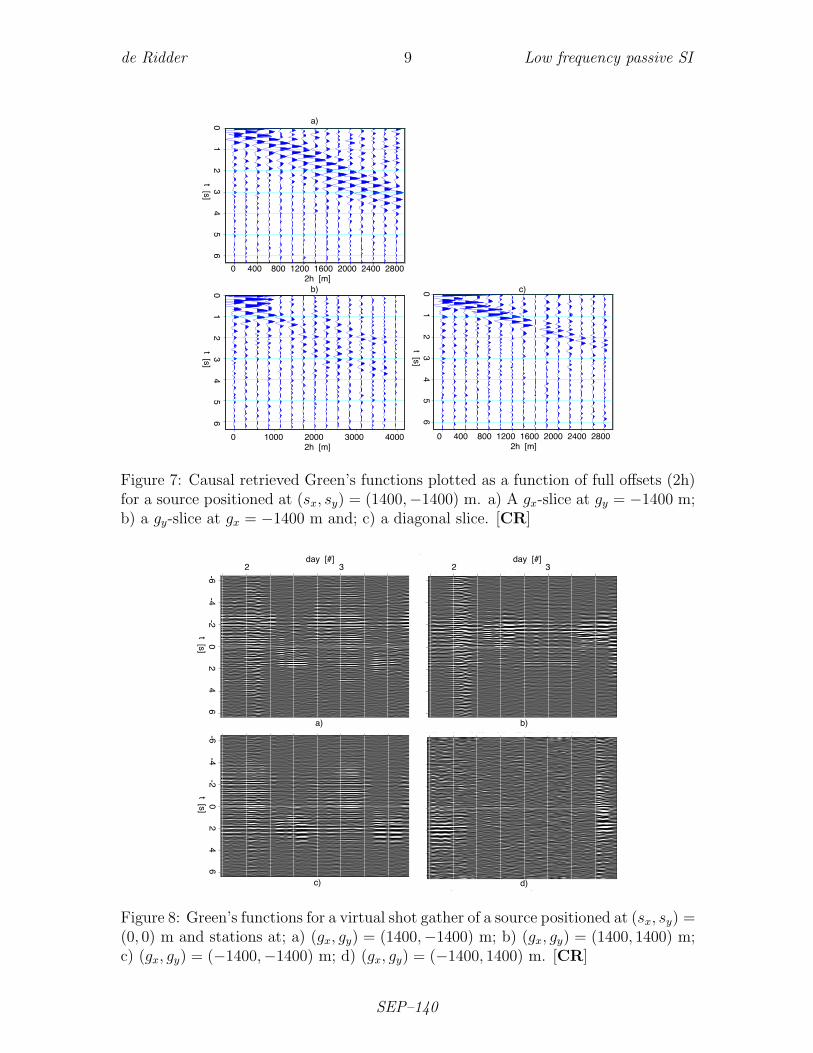
relation cube, correlating one hour of data was not sufficient to achieve convergencefor a Green’s function along the long offsets of the diagonal slice. For the smalleroffsets along gx and gy-slices, one hour of data was sufficient to achieve reasonableconvergence. The move-out of the arrivals indicate a velocity of approximately 1000m/s.

The quality of the retrieved Green’s functions depends on the portion of data usedand the directionality in the ambient seismic field. To illustrate this, a correlationwas computed using each hour of data, for a virtual source at (sx, sy) = (0, 0) mand stations at the 4 corners of the array. The gathers are shown in Figure 8. Thetime asymmetry of the retrieved result can be linked to the directionality of theambient seismic field. For example, for the retrieved signals on day 1 using the datarecorded from 20:00 to 21:00, the energy in the correlations is dominantly causal forthe station in the south and dominantly acausal for the station in the north, whichis consistent with the observation that energy is traveling southwards for this timeperiod. A high concentration of energy arriving at a station focused at approximatelyt = ±2 s corresponds to a good convergence rate. The observed convergence ratescan be related to the strength of the ambient seismic field (see the frequency spectraof figure 2). Notice the crisp causal Green’s functions for daylight hours arriving atthe south station.

SPATIAL VARIABILITY AND DISPERSION

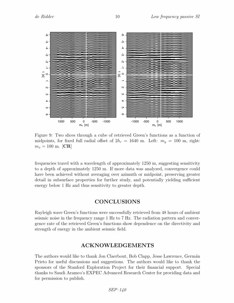
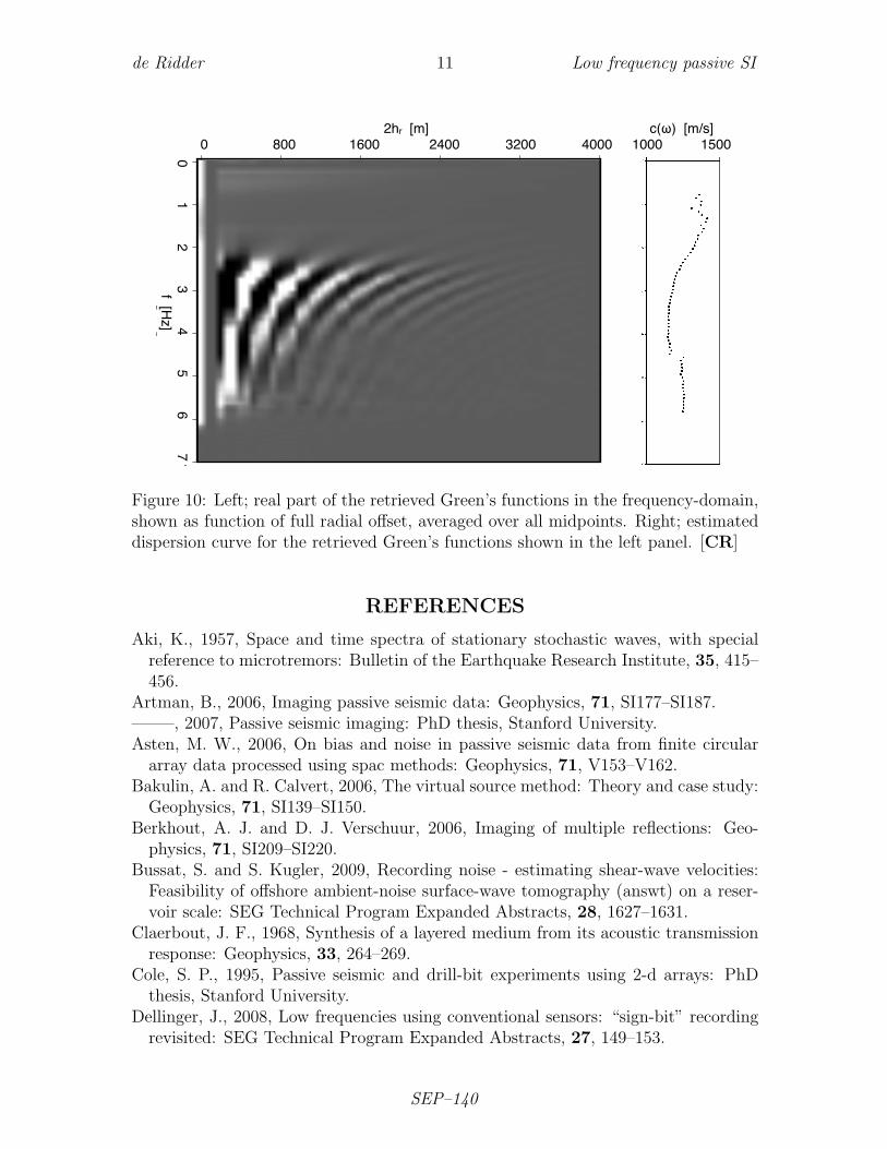
Stacking is required to further analyze the obtained virtual seismic survey. First,each spatial axis in the virtual seismic survey is transformed from source-geophonecoordinates (s, g), to midpoint (half)offset coordinates (m, h). Then, under a local1D approximation, the offset coordinates (hx, hy) are transformed into cylindricalcoordinates and stacked over azimuth. The result is a virtual seismic survey at eachmidpoint, as a function of radial offset hr. This result is analogous to the spatial auto-correlation of Aki (1957) (Asten, 2006; Yokoi and Margaryan, 2008). To investigateif there is any spatial variability despite the local 1D approximation, the retrievedGreen’s function for a full radial offset of 2hr = 1640 m are displayed in Figure 9for two midpoint slices at my = 100 m and mx = 100 m. Notice the Rayleigh wavesarrive earlier for midpoints with negative mx and positive my than for midpointswith positive mx and negative my. This is consistent with the observation of highervelocities on the east side than on that the west end of the array, see previous section.Notice how the dominant phase of the arrival-train travels with a different velocitythan the group velocity, indicating dispersion.The fundamental mode of a Rayleigh surface wave is represented by a zero-orderBessel function of the first kind, stretched by phase velocity, station distance andfrequency (Aki, 1957; Okada, 2003). In Figure 10, this is observed in a frequency rangebetween 1.5 Hz and 6 Hz, for retrieved Rayleigh waves averaged over all midpoints inthe array. The jump in the dispersion curve at 4.5 Hz is caused by a poor interpolationtechnique in the rotation from Cartesian to cylindrical offsets. The lowest retrieved

SEP–140

de Ridder 8 Low frequency passive SI

t = 2.5s

t = 2.0s

t = 1.5s

t = 1.0s

t = 0.5s

t = 0.0st = 0.0s

t = -2.0s

t = -2.5s

gy [km]-1 0 1

gy [km]-1 0 1

1 0 -1gx [km

]1 0 -1

gx [km

]1 0 -1

gx [km

]1 0 -1

gx [km

]1 0 -1

gx [km

]1 0 -1

gx [km

]

t = -1.5s

t = -1.0s

t = -0.5s

Figure 6: Snap shots of a movie of the acausal (left) and causal (right) parts ofretrieved Green’s functions for a virtual source at (sx, sy) = (0, 0) m. [NR]

SEP–140

de Ridder 9 Low frequency passive SI

0 1 2 3 4 5 6t [s]

0 1 2 3 4 5 6t [s]

0 1 2 3 4 5 6t [s]

0 400 800 1200 1600 2000 2400 28002h [m]

0 400 800 1200 1600 2000 2400 28002h [m]

0 1000 2000 3000 40002h [m]

a)

b) c)

Figure 7: Causal retrieved Green’s functions plotted as a function of full offsets (2h)for a source positioned at (sx, sy) = (1400,−1400) m. a) A gx-slice at gy = −1400 m;b) a gy-slice at gx = −1400 m and; c) a diagonal slice. [CR]

-6 -4 -2 0 2 4 6t [s]

-6 -4 -2 0 2 4 6t [s]

day [#]2 3

day [#]2 3

a) b)

c) d)

Figure 8: Green’s functions for a virtual shot gather of a source positioned at (sx, sy) =(0, 0) m and stations at; a) (gx, gy) = (1400,−1400) m; b) (gx, gy) = (1400, 1400) m;c) (gx, gy) = (−1400,−1400) m; d) (gx, gy) = (−1400, 1400) m. [CR]

SEP–140

de Ridder 10 Low frequency passive SI

-6 -5 -4 -3 -2 -1 0 1 2 3 4 5 6t [s]

-6 -5 -4 -3 -2 -1 0 1 2 3 4 5 6t [s]

1000 500 0 -500 -1000mx [m]

-1000 -500 0 500 1000my [m]

Figure 9: Two slices through a cube of retrieved Green’s functions as a function ofmidpoints, for fixed full radial offset of 2hr = 1640 m. Left: my = 100 m, right:mx = 100 m. [CR]

frequencies travel with a wavelength of approximately 1250 m, suggesting sensitivityto a depth of approximately 1250 m. If more data was analyzed, convergence couldhave been achieved without averaging over azimuth or midpoint, preserving greaterdetail in subsurface properties for further study, and potentially yielding sufficientenergy below 1 Hz and thus sensitivity to greater depth.

CONCLUSIONS

Rayleigh wave Green’s functions were successfully retrieved from 48 hours of ambientseismic noise in the frequency range 1 Hz to 7 Hz. The radiation pattern and conver-gence rate of the retrieved Green’s functions show dependence on the directivity andstrength of energy in the ambient seismic field.

ACKNOWLEDGEMENTS

The authors would like to thank Jon Claerbout, Bob Clapp, Jesse Lawrence, GermanPrieto for useful discussions and suggestions. The authors would like to thank thesponsors of the Stanford Exploration Project for their financial support. Specialthanks to Saudi Aramco’s EXPEC Advanced Research Center for providing data andfor permission to publish.

SEP–140

de Ridder 11 Low frequency passive SI

2hr [m]0 800 1600 2400 3200 4000

0 1 2 3 4 5 6 7 f [H

z]

c(ω) [m/s]1000 1500

Figure 10: Left; real part of the retrieved Green’s functions in the frequency-domain,shown as function of full radial offset, averaged over all midpoints. Right; estimateddispersion curve for the retrieved Green’s functions shown in the left panel. [CR]

REFERENCES

Aki, K., 1957, Space and time spectra of stationary stochastic waves, with specialreference to microtremors: Bulletin of the Earthquake Research Institute, 35, 415–456.

Artman, B., 2006, Imaging passive seismic data: Geophysics, 71, SI177–SI187.——–, 2007, Passive seismic imaging: PhD thesis, Stanford University.Asten, M. W., 2006, On bias and noise in passive seismic data from finite circular

array data processed using spac methods: Geophysics, 71, V153–V162.Bakulin, A. and R. Calvert, 2006, The virtual source method: Theory and case study:

Geophysics, 71, SI139–SI150.Berkhout, A. J. and D. J. Verschuur, 2006, Imaging of multiple reflections: Geo-

physics, 71, SI209–SI220.Bussat, S. and S. Kugler, 2009, Recording noise - estimating shear-wave velocities:

Feasibility of offshore ambient-noise surface-wave tomography (answt) on a reser-voir scale: SEG Technical Program Expanded Abstracts, 28, 1627–1631.

Claerbout, J. F., 1968, Synthesis of a layered medium from its acoustic transmissionresponse: Geophysics, 33, 264–269.

Cole, S. P., 1995, Passive seismic and drill-bit experiments using 2-d arrays: PhDthesis, Stanford University.

Dellinger, J., 2008, Low frequencies using conventional sensors: “sign-bit” recordingrevisited: SEG Technical Program Expanded Abstracts, 27, 149–153.

SEP–140

de Ridder 12 Low frequency passive SI

Dellinger, J. A. and J. Yu, 2009, Low-frequency virtual point-source interferometryusing conventional sensors: 71st Meeting, European Associated of Geoscientistsand Engineers, Expanded Abstracts, Expanded Abstracts, X047.

Dragonov, D., K. Wapenaar, W. Mulder, J. Singer, and A. Verdel, 2007, Retrieval ofreflections from seismic background-noise measurements: Geophys. Res. Let., 34,L04305–1 – L04305–4.

Fu, Q. and Y. Luo, 2009, Locating micro-seismic epicenters in common arrival timedomain: SEG Technical Program Expanded Abstracts, 28, 1647–1651.

Jervis, M. and S. N. Dasgupta, 2009, Recent mcroseismic monitoring results from vspand permanent sensor deployments in saudi arabia: EAGE Workshop on PassiveSeismic, Expanded Abstracts, A10.

Landes, M., N. M. Shapiro, S. Singh, and R. Johnston, 2009, Studying shallow seafloorstructure based on correlations of continuous seismic records: SEG Technical Pro-gram Expanded Abstracts, 28, 1693–1697.

Okada, H., 2003, The microtremor survey method. Geophysical Monograph, No. 12:Society of Exploration Geophysicists.

Schuster, G. T., J. Yu, J. Sheng, and J. Rickett, 2004, Interferometric/daylight seismicimaging: Geophys. J. Int., 157, 838–852.

Schuster, G. T. and M. Zhou, 2006, A theoretical overview of model-based and cor-relation based redatuming methods: Geophysics, 71, SI103–SI110.

Wapenaar, K., 2004, Retrieving the elastodynamic Green’s function of an arbitraryinhomogeneous medium by cross correlation: Phys. Rev. Lett., 93, 254301–1 –254301–4.

Xiao, X., Y. Luo, Q. Fu, M. Jervis, S. Dasgupta, and P. Kelamis, 2009, Locate micro-seismic by seismic interferometry: EAGE Workshop on Passive Seismic, ExpandedAbstracts, A22.

Yokoi, T. and S. Margaryan, 2008, Consistency of the spatial autocorrelation methodwith seismic interferometry and its consequence: Geophysical Prospecting, 56,435–451.

SEP–140