The Astrophysical Journal, 704:196–210, 2009 October 10 doi:10.1088/0004-637X/704/1/196C© 2009. The American Astronomical Society. All rights reserved. Printed in the U.S.A.

LOW MACH NUMBER MODELING OF TYPE IA SUPERNOVAE. IV. WHITE DWARF CONVECTION

M. Zingale1, A. S. Almgren

2, J. B. Bell

2, A. Nonaka

2, and S. E. Woosley

31 Department of Physics & Astronomy, Stony Brook University, Stony Brook, NY 11794-3800, USA

2 Center for Computational Sciences and Engineering, Lawrence Berkeley National Laboratory, Berkeley, CA 94720, USA3 Department of Astronomy & Astrophysics, The University of California, Santa Cruz, Santa Cruz, CA 95064, USA

Received 2009 May 22; accepted 2009 August 24; published 2009 September 21

ABSTRACT

We present the first three-dimensional, full-star simulations of convection in a white dwarf preceding a Type Iasupernova, specifically the last few hours before ignition. For these long-time calculations, we use our lowMach number hydrodynamics code, MAESTRO, which we have further developed to treat spherical starscentered in a three-dimensional Cartesian geometry. The main change required is a procedure to map theone-dimensional radial base state to and from the Cartesian grid. Our models recover the dipole structure ofthe flow seen in previous calculations, but our long-time integration shows that the orientation of the dipolechanges with time. Furthermore, we show the development of gravity waves in the outer, stable portion ofthe star. Finally, we evolve several calculations to the point of ignition and discuss the range of ignition radii.

Key words: convection – hydrodynamics – methods: numerical – nuclear reactions, nucleosynthesis, abundances– supernovae: general – white dwarfs

1. INTRODUCTION

Modeling highly subsonic convection in stars requires al-gorithms designed for long time integration. In the low Machnumber approximation, we filter out sound waves while keep-ing the compressibility effects important to describing the flow.In our previous work (see Almgren et al. 2006a, henceforthPaper I, Almgren et al. 2006b, henceforth Paper II, andAlmgren et al. 2008, henceforth Paper III), we developed alow Mach number stellar hydrodynamics algorithm for reactingfull-star flows in order to study the convective phase of TypeIa supernovae (SNe Ia). In Paper I, we derived the low Machnumber equation set. In Paper II, we included the effects of heatrelease due to external sources and allowed for a time-dependentbackground state. In Paper III, we incorporated reactions intothe system and also allowed the background state to evolve in re-sponse to large-scale convection and large-scale heating. Here,we extend the algorithm to spherical full-star problems using athree-dimensional Cartesian grid geometry.

Our target application for this algorithm is the period ofconvection that precedes the ignition of SNe Ia. The standardmodel of a SN Ia involves a white dwarf in a binary systemaccreting from a normal companion, and approaching theChandrasekhar mass (see for example Hillebrandt & Niemeyer2000). The increase in the central temperature and densityaccompanying the accretion seed carbon burning in the core,which in turn drives convection in the star. This convective“simmering” phase can last centuries, slowly increasing the coretemperature of the white dwarf (Woosley et al. 2004; Wunsch &Woosley 2004). A similar starting condition might be achievedin merging white dwarfs if mass is added slowly enough toavoid ignition at the edge of the stars (Yoon et al. 2007).During this phase, fluid heated by reactions buoyantly risesand cools via expansion, exchanging heat with its surroundings.The extent of the convective region grows with increasingtemperature, eventually covering roughly the inner solar massof the star. Outside of the convective region, the star is stablystratified.

The continued increase in central temperature, coupled withthe extreme temperature sensitivity of the carbon reactions,

means that eventually the reactions proceed vigorously enoughthat a hot bubble cannot cool fast enough, and a burning frontis born. This happens for a temperature of about (7–8) × 108 K(Nomoto et al. 1984; Woosley 1990). This burning front willquickly propagate through the white dwarf, converting mostof the carbon/oxygen fuel to heavier elements, and releasingenough energy to unbind the star. However, exactly where inthe star the ignition takes place is still unknown. Among theearliest work to consider the role of buoyancy in off-centerignition were Garcia-Senz & Woosley (1995), Bychkov &Liberman (1995), and Niemeyer et al. (1996). Additionally,some multidimensional studies of the dynamics of the firstbubbles to ignite in a white dwarf have been done (Iapichinoet al. 2006; Zingale & Dursi 2007). These papers made thecase that we really need to understand whether the ignition isat the center or off-center. As calculations have become moresophisticated, it has only become more clear that the outcome ofthe explosion is extremely sensitive to exactly how the burningfronts are initiated (Gamezo et al. 2005; Jordan et al. 2008;Ropke et al. 2007; Garcıa-Senz & Bravo 2005).

Less work has been done on multidimensional modelingof the convective phase preceding the explosion. To date, nomultidimensional calculation of the convection in the whitedwarf has modeled the entire star. The major contributionsthus far are two-dimensional simulations of a 90◦ wedge ofthe star using an implicit hydrodynamics code (Hoflich &Stein 2002; Stein & Wheeler 2006), and a three-dimensionalanelastic calculation (Kuhlen et al. 2006) of the inner convectiveregion of the star. All of these calculations cut out a smallpart of the central region of the star to avoid the coordinatesingularity at the origin in spherical coordinates. Furthermore,the Kuhlen et al. calculation modeled the star out to a radiusof only 500 km, leaving out part of the convective zone andthe surrounding, stably stratified region. The calculations byHoflich & Stein (2002) found ignition near the center of thewhite dwarf, produced by the fluid flow converging toward thecenter, with convective velocities of about 100 km s−1. However,the ignition they see was likely affected by the converginggeometry of their computational domain. The three-dimensionalcalculations by Kuhlen et al. (2006) showed that the large-scale

196

No. 1, 2009 LOW MACH NUMBER MODELING OF SNe Ia. IV. 197

flow took on a dipole pattern, suggesting that off-center ignitionin an outflow on one side of the star might be favored. Theyalso investigated the role of rotation. Finally, recent calculationsshown in Woosley et al. (2007) used an anelastic method on aCartesian grid, avoiding the singularity in the center, but still cutout the outer part of the convective region and the convectivelystable region surrounding it. Here the dipole was once againseen.

As seen from the wide range of explosion outcomes inthe literature, realistic initial conditions are a critical part ofSNe Ia modeling. Only simulations of this convective phasecan yield the number, size, and distribution of the initial hotspots that seed the flame. Additionally, the initial turbulentvelocities in the star are at least as large as the laminar flamespeed (Hoflich & Stein 2002), so accurately representing thisinitial flow may be an important component to explosionmodels. Perhaps owing to a limited number of convectioncalculations, with few exceptions (Livne et al. 2005), nearly allexplosion models to date begin with a quiet (zero velocity) whitedwarf.

Our goal in this study is to demonstrate that we havedeveloped low Mach number hydrodynamics to the point wherewe can perform detailed calculations of the convective flowpreceding the explosion, and to begin to understand the nature ofthe dynamics. In this work, we model the entire star, includingthe region surrounding the convective zone. Recently, it hasbeen suggested (Piro & Chang 2008) that the dynamics at theinterface between the convective and stably stratified regions ofthe star may be important during the flame propagation phase.Only full star calculations can capture this part of the flow. Theresulting simulations can then form the basis for simulationsof the flame propagation to build a more detailed picture ofSNe Ia.

2. NUMERICAL METHODOLOGY AND SETUP

The basic idea of low Mach number hydrodynamics is toreformulate the fluid equations to filter out sound waves whileretaining the compressibility effects important to the problem—in this case, local compressibility effects due to burning, andlarge-scale effects due to the background stratification of thestar. A full derivation of the equations of low Mach numberhydrodynamics is presented in Papers I–III. Here we show thefinal equations and discuss adjustments needed for the sphericalstar. We recall that the use of low Mach number equations ratherthan the fully compressible equations enables the use of a timestep based on the fluid velocity rather than the sound speed;this allows a 1/M increase in the time step over traditionalcompressible codes, where the Mach number, M, represents theratio of fluid velocity to sound speed. During the convectivephase preceding the first flames in SNe Ia, we expect the Machnumber to be O(0.01), making a low Mach number algorithman appropriate choice.

We choose to discretize our three-dimensional grid usingCartesian rather than spherical coordinates in order to avoida coordinate singularity at the center of the star. This gives riseto the most notable difference from Paper III—the base stateis a one-dimensional radial profile and is not aligned with anyof the axes in the three-dimensional Cartesian grid. We referto this as a spherical geometry, reflecting the fact that the basestate is discretized in one-dimensional spherical coordinates.Throughout this paper, we refer to the Cartesian coordinates ofthe center of the star as (xc, yc, zc).

2.1. Equation Set

The formulation of our equations relies on the existenceof a base state density, ρ0(r), and pressure, p0(r), that arein hydrostatic equilibrium, ∇p0 = ρ0ger , where er is a unitvector pointing in the radial direction from the center of thestar. In spherical geometries, the gravitation acceleration, g(r),is computed solely using the base state density as

g(r) = −GMencl(r)

r2, (1)

with the mass enclosed within a radius r defined as

Mencl(r) = 4π

∫ r

0ρ0(r ′)r ′2dr ′. (2)

As we discuss in Section 2.4, we use a cutoff density, ρcutoff ,in our initial model. The star is mapped onto the grid downto this cutoff density, surrounded by an ambient medium. Incomputing Mencl, we stop contributing to Mencl once the densitydrops below ρcutoff .

In this paper, we reuse much of the notation from Paper III.The overbar represents the average of a quantity over a layer ofconstant radius in the star

φ(r) = 1

A(ΩH )

∫ΩH

φ(x) dA, (3)

where ΩH is a region at constant radius in the star, andA(ΩH ) ≡ ∫

ΩHdA. In this notation, x represents the Cartesian

coordinates on the three-dimensional grid, and r is the basestate radial coordinate centered at (xc, yc, zc). A subscript “0”represents a base state quantity. We compute er in a cell indexedby (i, j, k) with Cartesian coordinates (xi, yj , zk) as

er = xi − xc

rex +

yj − yc

rey +

zk − zc

rez, (4)

with r2 = (xi − xc)2 + (yj − yc)2 + (zk − zc)2, and ex , ey , and ez

being the unit vectors for the Cartesian coordinate system.In our previous work, the total fluid velocity, U, was decom-

posed into a local velocity field, U, and base state velocity, w0,as

U = U(x, t) + w0(r, t)er . (5)

The base state velocity is used to adjust the base state in responseto the heating on the grid. In Paper II, we demonstrated thatwhen the heating is large, expanding the base state is critical toaccurately modeling the flow.

In the current application, convection in the white dwarf, theheating is small until the flame ignites. Therefore, for these firstcalculations, we use a background state that is fixed in time.We will later quantify the extent to which this assumption ofa fixed background state is valid. This simplifies the evolutionequations, and we can now use U for U and w0 = 0.

The full state evolves according to

∂(ρXk)

∂t= −∇·(UρXk) + ρωk, (6)

∂U

∂t= −U·∇U − 1

ρ∇π − (ρ − ρ0)

ρger . (7)

Equation (6) is the species evolution equation, where Xk isthe mass fraction of species k, with the creation rate ωk

provided by the nuclear reaction network. The mass density,

198 ZINGALE ET AL. Vol. 704

ρ, is simply ρ =∑k(ρXk). For the velocity evolution equation(Equation (7)), π is the dynamic pressure resulting from theasymptotic expansion of the pressure in terms of the Machnumber. In Paper III, we also evolved the enthalpy for the solepurpose of getting the temperature to feed into the reactionnetwork. For this paper, we instead define the temperature fromρ, p0, and Xk. Our experience has shown that, with the sphericalgeometry, the discretization errors are minimized by using thehydrostatic, radial base state pressure to define temperature. Wewill revisit this in a future paper. This system of equations isidentical to that presented in Paper III, with U = U, w0 = 0,and ∂p0/∂t = 0.

The velocity field is subject to a constraint equation

∇·(β0U) = β0S, (8)

with

β0(r) = ρ0(0) exp

(∫ r

0

1

Γ1p0

∂p0

∂r ′ dr ′)

, (9)

where Γ1 is the average over a layer of d(log p)/d(log ρ) atconstant entropy, and

S = −σ∑

k

ξkωk +1

ρpρ

∑k

pXkωk + σHnuc. (10)

Here, pXk≡ ∂p/∂Xk|ρ,T ,Xj,j �=k

, ξk ≡ ∂h/∂Xk|p,T ,Xj,j �=k, pρ =

∂p/∂ρ|T ,Xk, and σ = pT /(ρcppρ), with pT ≡ ∂p/∂T |ρ,Xk

and cp ≡ ∂h/∂T |p,Xkbeing the specific heat at constant

pressure. In these derivatives, h is the specific enthalpy, definedin terms of the specific internal energy, e, pressure, and densityas h = e + p/ρ. Finally, Hnuc is the nuclear energy release (withunits of erg g−1 s−1) as computed from our reaction network.Physically, S represents the local compressibility effects dueto heat release from reactions and composition changes. Thepresence of the density-like quantity β0 inside the divergence inthe constraint captures the expansion of a parcel of fluid as itrises in the hydrostatically stratified star.

We refer the reader to the extensive comparisons with com-pressible algorithms in Papers I through III that demonstrate thevalidity of the low Mach number approximation. For the mostpart, the algorithm to evolve the star follows closely that de-scribed in Paper III. For the construction of the advective terms,the interface states are again constructed using a piecewise lin-ear unsplit Godunov scheme based on that of Colella (1990),but we now use the full corner-coupling scheme developed bySaltzman (1994). In the subsections below, we point out thedifferences for the present application.

2.2. Mapping

Since the one-dimensional radial base state is not alignedwith any of the axes in the three-dimensional Cartesian grid,the discretization of quantities that involve both the base stateand the full state becomes complicated. Various parts of thealgorithm (such as the averaging operations) require a mappingbetween the base state and the full state. Because the basestate is not aligned with the Cartesian coordinate axes, weare free to choose the base state resolution independent of theCartesian grid spacing. Numerical experimentation has shownthat setting the base state resolution, Δr, to be finer than theCartesian grid resolution, Δx, gives the best results. (Herewe assume Δx = Δy = Δz.) For the present simulations,we use 5Δr = Δx. We refer to the procedure that maps data

Figure 1. Cartesian grid and spherical base state (shown here in two dimensionsfor simplicity, using 2Δr = Δx). Here we represent the spherical base state asconcentric shells (black curved lines). Since the base state is not aligned withthe Cartesian grid, we need to map between the two configurations. The “+”symbols represent the Cartesian zone centers. In our mapping from the radialprofile to the Cartesian grid, the zones marked with the “×” symbol are assignedthe value from the gray-shaded radial bin.

from one dimension to three dimensions as fill_3d, and thecomplementary procedure that maps from three dimensions toone dimension as average.

Figure 1 shows the Cartesian grid overlaid by the sphericalbase state (for simplicity, the figure is drawn in two dimensionsusing 2Δr = Δx). The fill_3d procedure computes thedistance of the center of cell indexed by (i, j, k) from the centerof the star:

r =√

(xi − xc)2 + (yj − yc)2 + (zk − zc)2. (11)

We use this radius to find the corresponding radial bin asn = int(r/Δr) (here, our convention is to use 0-based indexingfor the base state). We can then initialize a Cartesian cell quantityq from its corresponding base state quantity, q0, as qi,j,k = q0,n.

For the average process, we first define a coarseone-dimensional radial array with Δrc = Δx. Then, for eachcell indexed by (i, j, k), we again compute the radius, r, asabove, and define the index of the corresponding coarse radialbin, nc = int(r/Δrc). We define q0,nc as the average of all theqi,j,k whose Cartesian cell centers map into the coarse radialbin nc. Next, we construct edge-centered states on the coarseradial bin using the fourth-order approximation, q0,nc+1/2 =(7/12)(q0,nc + q0,nc+1) − (1/12)(q0,nc−1 + q0,nc+2). Finally, foreach coarse radial bin, we construct a quadratic profile usingq0,nc−1/2, q0,nc and q0,nc+1/2. This is based on the interpolatingpolynomial used by the PPM scheme to find edge states (Colella& Woodward 1984). Specifically, for ncΔrc � r � (nc + 1)Δrc,the interpolating polynomial is

q0(r) = q0,nc−1/2 + ξ (r){Δqnc + q6,nc [1 − ξ (r)]

}, (12)

with

ξ (r) = r − ncΔrc

Δrc, (13)

No. 1, 2009 LOW MACH NUMBER MODELING OF SNe Ia. IV. 199

Δqnc = q0,nc+1/2 − q0,nc−1/2, (14)

and

q6,nc = 6

[q0,nc − 1

2

(q0,nc+1/2 + q0,nc−1/2

)]. (15)

We note that since we are not evolving the base state in thesimulation presented here, the feedback from the full state tothe base state through average is limited to computing Γ1, asneeded for updating β0.

2.3. Microphysics

We use the general stellar equation of state described byTimmes & Swesty (2000) and Fryxell et al. (2000), which in-cludes contributions from electrons, ions, and radiation. Forthese calculations, we include the effects of Coulomb correc-tions included in the publicly available version of this EOS(Timmes 2008).

Our reaction network is unchanged from Paper III, and isa single-step 12C +12 C reaction using screening as describedin Graboske et al. (1973), Weaver et al. (1978), Alastuey &Jancovici (1978), and Itoh et al. (1979), resulting in 24Mg ash.We release the energy corresponding to the binding energydifference between the magnesium ash and carbon fuel. Paper IIIprovides full details on how the reaction network is solved.Our only change from the implementation there is that we nowupdate the temperature at the end of the reaction step. Finally,we note that we do not call the reaction network for densitiesbelow ρcutoff .

We note that by integrating the reaction rate equation, weare dealing with reactions differently than Kuhlen et al. (2006).There, an analytic approximation to the reaction rate was usedand evaluated given a temperature and density. Our methodextends more easily to a full reaction network. A seconddifference is that Kuhlen et al. (2006) burned to a mix of neonand magnesium, leading to a slightly lower energy release. Thisdifference may affect the timescales we see in the calculation,but we do not expect it to introduce qualitative differences.

2.4. Initial Model

We begin with an initial one-dimensional white dwarf modelproduced with the stellar evolution code, Kepler (Weaveret al. 1978). This model was evolved to the point where thecentral temperature is 6 × 109 K, and the central density is2.6 × 109 g cm−3. The composition is about half 12C and half16O, with a small amount (< 0.5%) of ash in the center of thestar. The total mass of the star is 1.382 M�.

We follow the procedure outlined in Zingale et al. (2002) toconvert the initial model from the one-dimensional Lagrangianmesh used by Kepler to the uniformly zoned Eulerian grid usedin our calculation. It is important that the initial model satisfyhydrostatic equilibrium discretely with our equation of stateon the base state grid we use for our simulation. In particular,we want to enforce the following discretization of hydrostaticequilibrium:

p0,i+1 − p0,i = 1

2Δr(ρ0,i + ρ0,i+1)gi+1/2. (16)

Hydrostatic equilibrium alone does not specify our initial model;therefore, we must also specify the initial temperature. Inthe interior of the star, where convection dominates, constantentropy is a good approximation. We use this constraint together

Figure 2. Initial model used for the full star convection calculation. The top panelshows the density, and the bottom panel shows the temperature. In both panels,the vertical dotted gray line represents the location of the low density cutoff—data outside of this cutoff are not used by our calculations. The vertical dashedgray line indicates where our sponge forcing term begins. For the temperatureplot, the solid line represents the initial model used in our calculation, andthe dashed line represents the temperature structure for a completely isentropicmodel.

with Equation (16) and the equation of state to find thetemperature, density, and pressure throughout the inner regionof the star. For the composition, we use the profile provided bythe Kepler model, but since we are using a reduced network, wegroup together the 20Ne and 24Mg ash into a single compositionvariable.

The convective region is surrounded by an outer, convectivelystable region. When the isentropic temperature profile dropsbelow the temperature provided by the Kepler model, we switchto using the Kepler temperature. Figure 2 shows our finaltemperature profile, along with a completely isentropic modelfor reference. The departure of the two temperature curves marksthe boundary of the convective region. The mass of the innerisentropic region of the star is 1.131 M�. We note that the spatialextent of the convective zone in the white dwarf is somewhatuncertain. Different assumptions about the accretion historyof the white dwarf would lead to different mass convectionzones.

Overall, this procedure results in a slight adjustment of thestructure of the star compared to the initial Kepler model. The

200 ZINGALE ET AL. Vol. 704

resulting model serves as the initial base state for our calculation.As discussed in Papers II and III, outside of the star we cannotbring the density down to arbitrarily small values, as that wouldresult in a velocity field that would too severely restrict the timestep (a consequence of our constraint equation). In practice, weimpose a cutoff at a moderately small density, ρcutoff , and set thedensity to this constant value outside of the star. For the maincalculation presented here, we choose ρcutoff = 3 × 106 g cm−3.While this may sound high, we note that the mass of the starenclosed by ρcutoff is 1.378 M�—a 0.2% difference from thetotal mass of the star. We note also that as in Paper III, we usean anelastic cutoff, the density below which the coefficient, β0,of our velocity constraint is defined by keeping β0/ρ0 constant.In this paper, we always set the anelastic cutoff to be ρcutoff .

The initial three-dimensional state is set by using the fill_3droutine in Section 2.2 to interpolate ρ0, p0, Xk,0, and T0 toeach cell center. The initial velocity field is not as well defined.The one-dimensional stellar evolution code used mixing lengththeory to describe convective mixing in the interior of the star.When we map the model onto our three-dimensional grid, thereis a region that is convectively unstable (corresponding to theregion in Figure 2 where r < 1.0×108 cm). However, there is notenough information in the one-dimensional model to initializea three-dimensional velocity field that correctly represents theconvective field.

If we start with zero initial velocity, then at t = 0 the reactionsnear the core generate a large amount of energy, and the highlynonlinear form of the reaction rate means that the energy releasequickly grows. Without an initial velocity field to advect someof this energy away from the core, the energy generation growstoo quickly, and an unphysical runaway occurs. However, bystarting with an initial nonzero velocity field, our simulationvery quickly finds a convective velocity field that balances theenergy generation at the core. Thus, we define a set of Fouriermodes

C(x)l,m,n = cos

(2πlx

σ+ φ

(x)l,m,n

)(17a)

C(y)l,m,n = cos

(2πmy

σ+ φ

(y)l,m,n

)(17b)

C(z)l,m,n = cos

(2πnz

σ+ φ

(z)l,m,n

), (17c)

and

S(x)l,m,n = sin

(2πlx

σ+ φ

(x)l,m,n

)(18a)

S(y)l,m,n = sin

(2πmy

σ+ φ

(y)l,m,n

)(18b)

S(z)l,m,n = sin

(2πnz

σ+ φ

(z)l,m,n

), (18c)

where σ is the characteristic scale of the perturbation, and theφ

{x,y,z}l,m,n are randomly generated phases between [0, 2π ]. We then

compute the total contribution to the velocity perturbation fromthe modes as

u′ =3∑

l=1

3∑m=1

3∑n=1

1

Nl,m,n

[−γl,m,nmC(x)l,m,nC

(z)l,m,nS

(y)l,m,n

+ βl,m,nnC(x)l,m,nC

(y)l,m,nS

(z)l,m,n

](19a)

v′ =3∑

l=1

3∑m=1

3∑n=1

1

Nl,m,n

[γl,m,nlC

(y)l,m,nC

(z)l,m,nS

(x)l,m,n

− αl,m,nnC(x)l,m,nC

(y)l,m,nS

(z)l,m,n

](19b)

w′ =3∑

l=1

3∑m=1

3∑n=1

1

Nl,m,n

[−βl,m,nlC(y)l,m,nC

(z)l,m,nS

(x)l,m,n

+ αl,m,nmC(x)l,m,nC

(z)l,m,nS

(y)l,m,n

], (19c)

where αl,m,n, βl,m,n, and γl,m,n are randomly generated ampli-tudes between [−1, 1], and Nl,m,n =

√l2 + m2 + n2 is the nor-

malization,A perturbational velocity field is then computed as

u′′ = Au′

2

[1 + tanh

(rpert − r

d

)](20a)

v′′ = Av′

2

[1 + tanh

(rpert − r

d

)](20b)

w′′ = Aw′

2

[1 + tanh

(rpert − r

d

)], (20c)

where the tanh profile gradually cuts off the perturbationat a radius rpert with a transition thickness d. Finally, theinitial velocity field is computed by applying the projection to(u,′′ v,′′ w′′) to ensure that it satisfies the divergence constraint.We pick the amplitude, A, to be small, and independent of thevelocities used in the one-dimensional stellar evolution model.Once the flow field is established, we expect the details of theinitial velocity field to be forgotten. This is an area we willexplore in a subsequent paper.

Throughout the calculation, we solve the reaction networkto compute the energy release that drives the convection. Bystarting at a low initial central temperature, we thus expect arealistic flow field to build up over time as the central tem-perature increases from the reactions. In this respect, we differfrom the initialization procedure used in Kuhlen et al. (2006).In their anelastic approximation, they carried the perturbationaltemperature separately from the base state temperature, and toinitialize the flow field they evaluated the carbon burning heat-ing term using only the base state temperature. By excluding theperturbational temperature, they left out the nonlinear feedbackin the extremely temperature-sensitive carbon reaction rate, andtherefore built a flow field without the chance of runaway. Oncethe flow field was established, they fed the temperature pertur-bations back into the reaction rate to watch the runaway.

2.5. Sponging

As described in Paper III, we use a sponge to damp thevelocities outside of our region of interest. We use the samefunctional form here, with the velocity forcing given by

Unew = Uold − Δt κfdampUnew, (21)

No. 1, 2009 LOW MACH NUMBER MODELING OF SNe Ia. IV. 201

Figure 3. Inner sponge function, fdamp, as a function of radius for ρcutoff =3 × 106 g cm−3 (solid line), and the outer sponge function for D = 5 × 108 cmand a 3843 grid (dashed).

where κ is a frequency. For all results presented here, we useκ = 10 s−1. The sponge factor has the form

fdamp =

⎧⎪⎨⎪⎩

0 if r < rsp1

2

{1 − cos

[π

(r − rsp

rtp − rsp

)]}if rsp � r < rtp.

1 if r � rtp.(22)

The quantity rsp represents the radius where the spongingterm gradually begins to turn on, and is set to the radiuscorresponding to 10·ρcutoff . The top of the sponge, rtp, wherethe sponge is in full effect is set as rtp = 2rmd − rsp, with rmdset to the radius corresponding to the ρcutoff . As noted above,we use a ρcutoff = 3 × 106 g cm−3 for these calculations,so the corresponding density where our sponging begins is3 × 107 g cm−3. Based on our initial model, 1.320 M� ofthe star is contained within rsp—the sponge only affects thevery outer portion of the star. Figure 2 shows the location ofrsp for our initial model—we see that it is well outside theconvectively unstable region. Figure 3 shows fdamp versus r forρcutoff = 3 × 106 g cm−3.

This sponge is effective in damping the velocities at the edgeof the star. Our domain is D = 5 × 108 cm on a side, sothe distance from the center of the star along one of thecoordinate axes to the edge of the domain is 2.5 × 108 cm. Thedistance from the center to a corner of the domain is

√3 larger.

Because we are placing a spherical star in a cubic domain, wefound that we need an additional sponge to damp the velocitiesin the outer corners of the domain—well outside of the star.We define an outer sponge of the same form as above, butwith rtp = D/2 and rsp = rtp − 4Δx, where Δx is the gridspacing, and κ set to 10 times the value of the inner sponge.This additional sponge is included in the momentum equationin the same fashion as the inner sponge. Figure 3 shows theprofile of this additional sponge as well.

3. RESULTS

Our main goal in these simulations is to study the convectionin the white dwarf up to the point of ignition. In this section,we present results for our main 3843 convection calculation,supporting calculations with lower resolution, as well as a testproblem. In each case, the code was run with an advective CFLnumber of 0.5 with the star centered in a domain 5 × 108 cm ona side.

3.1. Test Problem: Isentropically Stratified Star

To test the interaction between the spherical base state andthe three-dimensional Cartesian representation of the star, weperform a simple advection test with an analytic solution. First,we construct a completely isentropic initial model. This isachieved by picking a central density of 2.6 × 109 g cm−3 anda central temperature of 6 × 108 K, and a uniform compositionof 0.3 12C and 0.7 16O, and integrating outward using ourhydrostatic equilibrium constraint, Equation (16), and forcingthe entropy to be constant through the equation of state. Weinitialize the full state using the isentropic base state with noperturbations. We also set β0 = ρ0 discretely (which is trueanalytically for an isentropic base state and constant Γ1), anddisable all reactions and heating. The constraint is now identicalto the anelastic constraint, ∇ · (ρ0U ) = 0.

Under these conditions, the continuity equation becomes

∂ρ

∂t= −∇ · (ρU ) = −∇ · (ρ0U ) = 0, (23)

using the fact that ρ = ρ0 initially, and the anelastic constraint.As a result, we see that the density should remain constant inthe star regardless of the velocity field.

This provides a means to test our mapping procedure. If westart with an isentropically stratified star and seed a randomvelocity field, the density should not change with time. Forour test, we start with a random velocity field described byEquation (26). For the amplitude of the perturbation, we setA = 107 cm s−1—this is typical of the highest velocities weexpect to see in our convection calculations. For the size of theperturbation, we set rpert = 5 × 107 cm—this value representsabout half the size of the expected convective region in thewhite dwarf. Finally, we set the characteristic wavelength ofthe perturbation, σ = 107 cm. We make the transition betweenthe perturbation and the ambient star sharp, effectively smallerthan our grid resolution, setting d = 105 cm. The resolutionis 3843, the same as that used in the main calculation in thefollowing section.

To assess the change in density with time, we will look at theaverage density, 〈ρ〉, as a function of radius, and the deviationof the density as a function of radius, δρ. We define these as

〈ρ〉r = 1

NΩr

∑Ωr

ρ, (24)

where Ωr is the set of cells in the computational domain whosecenter falls within the radial bin at radius r, and NΩr is thenumber of cells in Ωr . The rms fluctuations are

(δρ)r =⎡⎣ 1

NΩr

∑Ωr

(ρ − ρ0)2

⎤⎦

1/2

. (25)

202 ZINGALE ET AL. Vol. 704

Figure 4. (δρ)r /〈ρ〉r vs. r for the test problem at 3 times. We see that the relativechange in density resulting from a large amplitude velocity perturbation is small.

Here we recognize that the base state density, ρ0, representsthe average density at a given radius. We compute and store(ρ −ρ0) for every zone in our computational domain directly inthe code as the simulation runs, and then compute (δρ)r usingEquation (33) with a radial bin spacing Δr = Δx—this ensuresthat no interpolation is needed to fill radial cells.

Figure 4 shows a plot of (δρ)r/〈ρ〉r versus r at several times.By normalizing to the average density, 〈ρ〉r , we are seeing ameasure of the relative error in the density from our advectionscheme. As the plot shows, even after 1500 s of evolution,the error at the center of the star is < 10−11. Once we areoutside of the star r > 2 × 108 cm, the error rises, but stillstays below 5 × 10−9 everywhere. This demonstrates that ouralgorithm accurately preserves ∂ρ/∂t = 0 in the limiting caseof an isentropic model with no heating and β0 = ρ0.

3.2. Convection in a White Dwarf

We model convection in the white dwarf by mapping theinitial model described in Section 2.4 onto our Cartesian grid.For the initial velocity field, we use A = 105 cm s−1, d =105 cm, rpert = 2 × 107 cm, and σ = 107 cm.

3.2.1. Diagnostics

To help us understand the character of the flow in ourcalculations, we make use of several diagnostic quantities.We define the region of interest of the domain, Ωstar, to bethose computational cells with ρ > ρcutoff , where we haveused ρcutoff = 3 × 106 g cm−3 unless otherwise specified.The diagnostics defined below are computed every time step, asthe code is running.

The peak temperature in the domain is simply

Tpeak = maxΩstar

{T }. (26)

As the temperature in the star increases considerably toward thecenter of the star, we expect the peak temperature to be close to(but not exactly equal to) the central temperature.

Motivated by previous results that suggest a dipole nature tothe flow (Kuhlen et al. 2006), we look at several diagnosticsbased on the radial fluid velocity. First, we define the radialvelocity to be vr = U·er . Then we compute components ofthe density-weighted average radial velocity in each coordinatedirection

〈vr〉x =∑NΩstar

ρvr

(x − xc

r

)/∑NΩstar

ρ, (27)

where r is the distance of a given zone from the center of the star,and NΩstar is the number of computational zones contained in thedomain Ωstar. We compute 〈vr〉y and 〈vr〉z analogously, using(y − yc) and (z − zc), respectively. The relative magnitudes ofthe components of 〈vr〉i tell us about the direction of any dipolenature to the flow. In particular, we can derive the directionalangles φ in the x–y plane, and θ as measured from the z-axis as

φ = tan−1

( 〈vr〉y〈vr〉x

)(28)

and

θ = tan−1

⎛⎝√

〈vr〉2x + 〈vr〉2

y

〈vr〉z

⎞⎠ . (29)

We could have instead computed the average radial velocitywithout a density weighting, but because we are summing overthe entire star (where ρ > ρcutoff), we are including the outerconvectively stable region in the average, where we do not expectto see much influence from the dipole. By density weighting,we are giving more weight to the center of the star, where theconvective pattern dominates.

Finally, to get a sense of scale for the radial velocity in thestar, we compute

(vr )peak = maxΩstar

{|vr |}. (30)

3.2.2. Long-term Convective Behavior

Our main result is a 3843 calculation of convection in a whitedwarf, starting from an initial model with a central temperatureof 6×108 K. Our computational domain is 5×108 cm on a side,giving us 13 km zones. Our goal is to follow the convection asreactions bring the central temperature up over 7 × 108 K andinto the regime of ignition.

As noted in Section 2.4, we started with a small velocityperturbation near the center of the star and the velocity otherwisezero. As the simulation begins, reactions heat the core of the star,and since the background of the star is isentropic, the heatedfluid at the core begins to buoyantly move radially outward.Figure 5 shows the magnitude of the vorticity (|∇ × U|) in thethree orthogonal slice planes through the center of the star atseveral different times. At early times, we see convective flowdeveloping near the center of the star. By 400 s, the convectiveflow has grown to fill the convectively stable region, and wesee gravity waves excited in the stable region above. The latertimes show the convective pattern continuing to strengthen, withsmall asymmetries in the vorticity moving through the innerconvective region. For most of the simulation, we see a sharpdistinction in the character of the flow at the boundary of theisentropic region in the star. However, toward the very end ofthe calculation, as shown in the very last pane of Figure 5, we

No. 1, 2009 LOW MACH NUMBER MODELING OF SNe Ia. IV. 203

Figure 5. Development of the convective flow in the 3843 calculation. Here we plot vorticity. The data scale is capped at 1.75 s−1, even though the maximum vorticitysteadily climbs as the simulation progresses, reaching over 13 s−1 by the last panel. From left to right, top to bottom, the panels show the vorticity at 50, 100, 200,400, 800, 1600, 3200, and 6400 s.

no longer see the separation between the two regions, and theconvective plumes appear to travel through the entire star.

Figure 6 shows contours of the radial velocity at four differenttimes. Qualitatively, these times represent the early period(panel a, 800 s), two intermediate snapshots (panels b andc, 3200 and 3420 s, respectively), and the very late stage ofthe calculation (panel d, 7132 s). Red color indicates fluidmoving radially outward, and blue color indicates fluid movingradially inward. The gray surface is drawn at a constant density(ρ = ρcutoff) and represents the surface of the star. Very early wesee the distinct asymmetric nature to the flow characteristic of adipole flow. The dipole is not nearly as symmetric as that shownin Kuhlen et al. (2006), perhaps due to differing resolutionor the inclusion of the stably stratified layer surrounding theconvective region in our study. In general, the outward movingfluid appears more coherent then the inward moving fluid.Comparing the images at different times, we see that the dipoledirection changes with time. Occasionally, the flow takes on amore organized form, with the inward moving fluid forming aconcentric ring around the outward flow, as shown in panel c.At the very late stages of the simulation (panel d), we see whatappears to be a breakdown in the distinction between the stableand unstable regions, with the flow much less organized andfilling most of the volume of the star. The narrow gap between

the velocity contours and the surface of the star at late timesarises from our sponging term. We look at the sensitivity of theresults to the position of the sponge in the following subsection.

To get a better feel for the change in direction of the dipole,we compute the spherical angles, θ and φ, from 〈vr〉i , as definedabove. Figure 7 shows these angles as a function of time. Wesee that both angles move through their full range many timesover the course of the simulation. We see that the characteristictimescale for φ to complete a circuit through 2π is between 500and 1000 s. At late times, it appears that the dipole is changingdirection with a faster period, especially in the θ plot.

Figure 8 shows the peak radial velocity, (vr )peak, inside thestar, as a function of time. We see that it slowly rises with time,with a typical peak radial velocity of ∼ 107 cm s−1. Takingthe convective region to have a radius of Rconv ∼ 108 cm,we define a lower bound to the convective turnover time of2Rconv/(vr )peak = 20 s.

Ignition will occur when the reactions proceed so strongly thathot, reacting bubbles are not quenched by adiabatic expansion inthe convective motions carrying the fluid away from the centerof the star. Since the 12C + 12C reaction rate is so stronglytemperature-sensitive, the peak temperature in the star servesas a good guide for observing the progression toward ignition.Figure 9 shows the peak temperature as a function of time for

204 ZINGALE ET AL. Vol. 704

Figure 6. Radial velocity shown at 4 different times: (a) 800 s; (b) 3200 s; (c) 3420 s; (d) 7131.79 s. The latter time corresponds to the point of ignition. Red contoursindicate outward moving fluid while blue contours indicate inward moving fluid. Two contour levels are used for each sign, ±1.2 × 106 cm s−1 and ±2 × 106 cm s−1.The gray contour is a surface of constant density, ρ = ρcutoff , marking the surface of the star.

this calculation. We see a short transient at the start of thecalculation where the temperature quickly rises and then settlesback down—this occurs from the nonlinear feedback of thetemperature into the reactions when the flow field is not yetfully developed. After a short amount of time, a convective flowfield develops that properly matches the energy generation at thecenter of the star, and the temperature settles into a long, gradualrise. About halfway through the calculation, we can clearlysee that the temperature rise is nonlinear, and the temperatureincrease accelerates toward the very end, up to the point ofignition. The inset in Figure 9 shows the behavior of Tpeak duringthe last 200 s.

The reactions dump energy into the star, and it heats upthroughout. Figure 10 shows the average temperature at a givenradius as a function of the radius at several different times. Aswe see, the temperature increases throughout the convectiveregion. At late times, we see a distinct change in the temper-ature structure at the boundary of the convective region. Thischange in the temperature structure corresponds to the penetra-tion of the vortical flow through the original boundary betweenthe stable and unstably stratified regions in the vortical plot(Figure 5) shown above. It is not clear how robust this change inthe character of the flow is to resolution—that is something thatwill be explored through higher resolution studies in the future.

No. 1, 2009 LOW MACH NUMBER MODELING OF SNe Ia. IV. 205

Figure 7. Spherical angles, θ and φ, computed from 〈vr 〉i as a function of timefor the 3843 calculation. The vertical dotted lines represent where the angle φ

crosses the 0◦–360◦ boundary, and are not really discontinuities. We see thatthe direction of the dipole changes constantly throughout the simulation.

Figure 8. Peak radial velocity as a function of time for the 3843 calculation.

It is also the case that those outer layers, near the transition to astably stratified fluid, are where we would expect the expansionof the star to be greatest, so we need to check if neglecting the

Figure 9. Maximum temperature in the white dwarf as a function of time forthe 3843 calculation. The temperature increase is highly nonlinear, ending atignition. To show detail, we restrict the vertical range of the plot to 8 × 108 K.The inset shows the structure of Tpeak during the last ∼200 s. We see large, butdamped excursions in central temperature just prior to ignition.

Figure 10. Average temperature as a function of radius in the white dwarf, shownat the initial time and three later times, for the 3843 convection calculation. Withtime, the energy dumped into the star by reactions causes the temperature toincrease throughout the star. The curve at 7132 s corresponds to the time ofignition.

base state evolution was warranted. Figure 11 shows (δρ)r/〈ρ〉rversus radius at several times. This is a measure of how muchexpansion of the star has taken place. If (δρ)r is large comparedto 〈ρ〉r , then the full state is carrying the expansion rather thanthe base state, and as we have shown in Paper II, this can lead to

206 ZINGALE ET AL. Vol. 704

Figure 11. (δρ)r /〈ρ〉r vs. r for the 3843 white dwarf convection problem atthree times. The curve at 7132 s corresponds to the time of ignition. We see thatat all times, (δρ)r /〈ρ〉r remains well below 1% everywhere inside the star.

inaccuracies. As Figure 11 shows, (δρ)r/〈ρ〉r is always below1%, indicating that the departure from the base state is small,and any expansion would be minimal. In each case, the curve at7132 s corresponds to the point is ignition, discussed below.

We can also look at the total kinetic energy in the star, whichwe compute as

K =∑Ωstar

ρ|U|2ΔxΔyΔz. (31)

At the point when the peak temperature reaches 8 × 108 K, thetotal kinetic energy inside the star is 6.24 × 1046 erg. To put thisin context, we can compare the gravitational potential energy ofthe star, defined from our base state as

U = −∫

Ωstar

GM(r)dM

r, (32)

with dM = 4πr2ρ0dr . For our model, the gravitationalpotential energy is −3.2 × 1051 erg. The internal energy ofthe gas is also quite large, Eint = 2.7 × 1051 erg, giving anenergy difference of ∼ −5×1050 erg that needs to be overcometo unbind the star. Therefore, kinetic energy release up to thepoint of ignition is a tiny fraction of what is needed to unbindthe star, as expected.

The 3843 calculation took 113,156 time steps to reach a sim-ulation time of 7131.8 s—at which point the peak temperaturehad risen to 8 × 108 K, and ignition shortly followed. Overall,the average time step is 0.063 s. At this same instant, the Machnumber, attained in the outer layers of the star, reached a value of0.079. Earlier in the calculation, the maximum Mach number inthe domain was considerably lower. For comparison, the highestsound speed in the star (at its center) is 9.5 × 108 cm s−1, whichwould give a corresponding time step of 7 × 10−4 s (assuming aCFL number of 0.5, and |U | cs , where cs is the sound speed).

3.2.3. Effect of ρcutoff

As we noted above, the behavior of the coefficient in ourconstraint term and the location of the sponge are set by the

Figure 12. Maximum temperature in the white dwarf as a function of time forthe two different choices of ρcutoff (106 g cm−3 and 3 × 106 g cm−3). Bothsimulations use a 2563 grid. Here we see excellent agreement between the twocases, indicating that the peak temperature is insensitive to our choice of ρcutoff .

density we refer to as ρcutoff . To assess the influence of ourchoice of ρcutoff , we perform a pair of simulations on a 2563 gridthat are identical except for the value of ρcutoff . For our controlcase, we use ρcutoff = 3 × 106 g cm−3, the value chosen for ourmain calculation. To explore the effects of lowering ρcutoff , wealso try a value of ρcutoff = 106 g cm−3. We note that the locationof the sponge in the momentum equation remains keyed to thechoice of ρcutoff , so with the lower value of ρcutoff , the locationof the start of the sponge moves outward from the center ofthe star. In terms of mass, ρcutoff = 106 g cm−3 means that themass of the star enclosed is 1.381 M�, compared to 1.378 M�with ρcutoff = 3 × 106 g cm−3. The location of the start ofthe sponge contains 1.363 M�, compared with 1.320 M� withρcutoff = 3 × 106 g cm−3.

Figure 12 shows Tpeak as a function of time for the twocalculations. As we see, the two curves track very well,indicating that the choice of ρcutoff has little influence on thetemperature behavior near the center of the star. The time atwhich final ignition occurs differs between these two cases byonly 38.4 s out of over 6000 s of evolution.

As noted above, the choice of ρcutoff is used to prevent thevelocities from growing too large as the fluid experiencesthe steep density gradient at the edge of the star. We note that thetime step the code takes with ρcutoff = 3 × 106 g cm−3 is 23%larger than with ρcutoff = 106 g cm−3. Thus, it is computationalfavorable to use the slightly higher value of the cutoff density.

3.2.4. Ignition

As the inset in Figure 9 shows, up to the point of ignition,the peak temperature rises rapidly, only to fall again, as a sparkfails to ignite. Figure 13 shows the temperature structure in thelast 500 s for the 3843 calculation and both 2563 calculations,shifted so the time of ignition lines up. All three runs show thepeak temperature fluctuating rapidly before ignition, indicatingsome hot spots failed to ignite. In each case, eventually, a hot spot

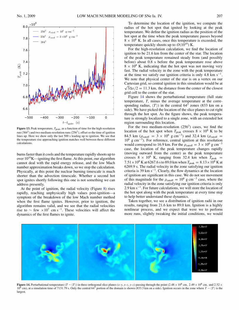
No. 1, 2009 LOW MACH NUMBER MODELING OF SNe Ia. IV. 207

Figure 13. Peak temperature, Tpeak, as a function of time for the high resolutionrun (3843) and two medium-resolution runs (2563), offset so the time of ignitionlines up. Here we show only the last 500 s leading up to ignition. We see thatthe temperature rise approaching ignition matches well between these differentcalculations.

burns faster than it cools and the temperature rapidly shoots up toover 1010K—igniting the first flame. At this point, our algorithmcannot deal with the rapid energy release, and the low Machnumber approximation breaks down, so we stop the calculation.Physically, at this point the nuclear burning timescale is muchshorter than the advection timescale. Whether a second hotspot ignites shortly following this one is not something we canaddress presently.

At the point of ignition, the radial velocity (Figure 8) risesrapidly, reaching unphysically high values post-ignition—asymptom of the breakdown of the low Mach number methodwhen the first flame ignites. However, prior to ignition, thealgorithm remains valid, and we see that the radial velocitiesrise to ∼ few ×107 cm s−1. These velocities will affect thedynamics of the first flames to ignite.

To determine the location of the ignition, we compute theradius of the hot spot that ignited by looking at the peaktemperature. We define the ignition radius as the position of thehot spot at the time when the peak temperature passes beyond8 × 108 K. In all cases, once this temperature is exceeded, thetemperature quickly shoots up to O(1010) K.

For the high-resolution calculation, we find the location ofignition to be 21.6 km from the center of the star. The locationof the peak temperature remained steady from (and possiblybefore) about 0.8 s before the peak temperature rose above8 × 108 K, indicating that the hot spot was not moving veryfast. The radial velocity in the zone with the peak temperatureat the time we satisfy our ignition criteria is only 4.8 km s−1.We note that physical center of the star is on a vertex on ourCartesian grid, so central ignition in this simulation would be at√

3Δx/2 = 11.3 km, the distance from the center of the closestgrid cell to the center of the star.

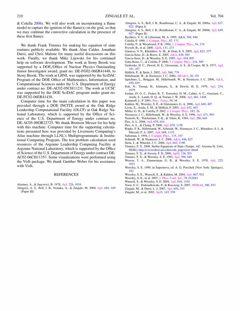
Figure 14 shows the perturbational temperature (full statetemperature, T, minus the average temperature at the corre-sponding radius, 〈T 〉) in the central 643 zones (833 km on aside). We have picked the location of the slice planes to cut rightthrough the hot spot. As the figure shows, the peak tempera-ture is strongly localized to a single zone, with an extended hotregion surrounding this location.

For the two medium-resolution (2563) cases, we find thelocation of the hot spot when Tpeak crosses 8 × 108 K to be84.5 km (ρcutoff = 3 × 106 g cm−3) and 32.4 km (ρcutoff =106 g cm−3). For reference, central ignition at this resolutionwould correspond to 16.9 km. For the ρcutoff = 3 × 106 g cm−3

case, the location of the peak temperature changes rapidly(moving outward from the center) as the peak temperaturecrosses 8 × 108 K, ranging from 32.4 km when Tpeak =7.51×108 K at 6267.6 s to 89.0 km when Tpeak = 8.13×108 K at6269.9 s. The radial velocity in the zone satisfying our ignitioncriteria is 39 km s−1. Clearly, the flow dynamics at the locationof ignition are significant in this case. We do not see movementof this magnitude for the ρcutoff = 106 g cm−3 case, where theradial velocity in the zone satisfying our ignition criteria is only2.9 km s−1. For future calculations, we will store the location ofthe hot spot along with the peak temperature at every time stepto help better understand these dynamics.

Taken together, we see a distribution of ignition radii in ourresults, ranging from 21.6 km to 89.0 km. Ignition is a highlynonlinear process, and we expect that were we to performmore runs, slightly tweaking the initial conditions, we would

Figure 14. Perturbational temperature (T −〈T 〉) in three orthogonal slice planes (x–y, x–z, y–z) passing through the point (2.48 × 108 cm, 2.49 × 108 cm, and 2.52 ×108 cm), at a simulation time of 7131.79 s. Only the central 643 portion of the domain is shown (833.3 km on a side). Ignition occurs in the zone where T − 〈T 〉 is thelargest.

208 ZINGALE ET AL. Vol. 704

Figure 15. Peak temperature, Tpeak, in the white dwarf as a function of timefor three different resolutions. We see that as we increase the resolution, thetemperature increase is slower. The lowest resolution case reaches ignitionvery quickly. Once it ignites, the peak temperature climbs to ∼ 1010 K almostinstantly. To show detail, we restrict the vertical range of the plot to 8 × 108 K.

observe different values, all of which sample the distributionfunction of possible ignition locations in the problem. Owingto the stochastic nature of the problem, to really understand theignition process requires performing a large number of slightlydifferent calculations to map out the distribution function.

3.2.5. Effect of Resolution

It has been suggested that the behavior of convectiveflow can dramatically change in character at high Rayleighnumber (Kadanoff 2001). In our simulation code, we donot explicitly add viscosity to the momentum equation(Equation (7)), so our Rayleigh number is determined by thenumerical viscosity inherent in our advection scheme. Further-more, the nature of the turbulence will depend on the Reynoldsnumber of the flow, which again in our simulations is deter-mined by numerical viscosity. Practically speaking, the way toincrease the effective Reynolds and Rayleigh numbers of thesimulation is to move to higher order advection methods and toincrease the resolution.

While no amount of resolution will bring our effectiveReynolds and Rayleigh numbers up to the O(1014) and O(1025)values, respectively, we expect in the true convecting whitedwarf (Woosley et al. 2004), it is interesting to look at howthe general results change with resolution. A second reasonto explore resolution is that it is not known what size regionwill ignite. One might imagine that a region the size of onlya few flame thicknesses needs to heat up to ignite a flame. Atthe central densities in the white dwarf, the flame thickness is

Figure 16. Peak radial velocity, (vr )peak, in the white dwarf as a function oftime for three different resolutions.

O(10−4 cm) (Timmes & Woosley 1992)—this is far below anyresolution that can be obtained by a large-scale simulation code.However, the flame will initially burn in place, growing until itis large enough (about 1 km) that buoyancy becomes significantand it begins to rise and deform (Zingale & Dursi 2007). Whilethis is still a smaller length scale than considered here, it is notout of reach with mesh refinement and larger computers.

To begin to understand the effect of resolution, we considerthree cases: 1283, 2563, and 3843, corresponding to physicalzone sizes of 39.1, 19.5, and 13.0 km, respectively. We notethat for the present study, computer resources prevent us fromconsidering a 5123 or higher case.

Figure 15 shows Tpeak versus time for the three differentresolutions. Immediately, we see that the 1283 case reachesignition much faster than the two higher resolution cases. Infact, from our starting temperature of 6 × 108 K, the highestresolution run takes more than twice as long in simulation timeto reach ignition. Also apparent in the coarsest resolution run isthat the temperature did not drop after the initial transient—thiscontributes to the faster overall evolution. Both of the higherresolution cases see a drop in the temperature after the initialtransient, as the developing velocity field carries the heatedfluid away from the center of the star. Close to ignition, the 2563

and 3843 runs show a similar slope in the Tpeak versus t curveshown in Figure 13. The peak radial velocity as a function oftime also shows differences between the resolutions, as shownin Figure 16. There does appear to be some convergence withresolution.

No. 1, 2009 LOW MACH NUMBER MODELING OF SNe Ia. IV. 209

4. CONCLUSIONS AND DISCUSSION

We have demonstrated that our simulation code, MAESTRO,is capable of following the convective flow in a white dwarfleading up to the ignition of a Type Ia supernova. We haveexplored the sensitivity of the results to resolution and to thechoice of low-density cutoff, ρcutoff . Our test problem showsthat discretizing the star on a Cartesian grid with a radial basestate leads to an accurate representation of the flow.

Over many convective turnover times, our simulations capturethe rise of the peak temperature in the white dwarf up toignition, recover the dipole nature of the convective flow firstshown in Kuhlen et al. (2006), and track the change in directionof the dipole. We see, for the first time in multidimensionalsimulations, the distinct change in the nature of the flow at theouter boundary of the convective region, as discussed in Piro &Chang (2008). The late time breakdown of this interface needsfurther investigation.

All of our models reached ignition. For the two medium-resolution runs, the ignition occurred at a radius of 32.4 and84.5 km. For the high-resolution run, it occurred at 21.6 km.These are the locations of the first flames. We note that this isa highly nonlinear problem, and small changes in the state ofthe star could affect the ignition process. To really understandthe statistical distribution of initial ignition points requiresrunning a suite of calculations, varying the initial model (centraldensity, size of initial convective region), and the initial state ofthe star. With an ensemble of such calculations, we could geta much better understanding of the ignition process. We alsoneed to understand how the ignition process differs with higherresolution.

A detailed comparison to Hoflich & Stein (2002) or Kuhlenet al. (2006) is difficult, because of the differing geometriesused. Hoflich & Stein (2002, henceforth HS) simulated a 90◦wedge in two dimensions, but cut out the innermost 13.7 km (intheir “extended computational domain” run). As we discussed inthe present calculation, the burning is strongly peaked near thecenter of the star, so cutting out the center would miss a great dealof the energy generation. It would also prevent the fluid fromflowing through the center of the star, which is the dominantpattern seen in the present calculation. Because HS used aspherical grid, and allowed the radial spacing to vary, thereis no single grid resolution for their simulation, but they statethat near the inner boundary, the grid resolution is “∼ 2 km”—about 6× finer than the uniform resolution we use throughoutthe star. In both their and our calculations, several hours of therunaway are followed leading up to the point of ignition (∼ 3 hrfor HS, ∼ 2 hr for our calculation). Also, in both cases, theignition takes place in a single zone. However, the details ofthe ignition differ, because HS have an inner boundary and awedge-shaped domain compression is generated that leads tothe ultimate ignition near the center. In our calculation, we haveflow through the center throughout the simulation. HS found theignition to take place at a radius of 27 km in their model, whichis within the range we report in our study. Furthermore, becausetheir initial model had a strong gradient in the carbon massfraction, with the outer portion of the star having a carbon massfraction of 0.4 and the core having a value close to 0.25 (seeHS, Figure 1), HS report that the expanding convective regionresults in an increase in the carbon mass fraction at the centerfrom 0.25 to 0.36. This is not the case in our model, where thecarbon burning caused a 0.5% decrease in the central carbonmass fraction over the time we modeled. HS quote convective

velocities between 40 and 120 km s−1 at ignition. In our case,the radial velocities were around 100 km s−1 for most of theevolution, rising to several times that just before ignition.

The calculation by Kuhlen et al. (2006, henceforth KWG)modeled the star in three dimensions, with an inner boundaryat 50 km, again cutting out the center of the star. They alsoput the outer boundary at 500 km, which is approximatelyhalfway through the convectively unstable region in the initialmodel (KWG and the present study use very similar initialmodels, generated from the Kepler stellar evolution code).Despite cutting out the center, KWG found that a large-scaledipole flow pattern dominates—similar to what we see (althoughwe note that they also did a rotating model, and saw the dipolebreak down). Unlike HS or the present calculation, KWG donot model the evolution continuously leading up to ignition, butrather model two snapshots in time, corresponding to centralwhite dwarf temperatures of 7 × 108 K and 7.5 × 108 K, withdurations of 70 and 41 s, respectively. This amounts to a fewturnover times (Kuhlen et al. 2006). It is difficult to compareresolution with KWG, as they use a spectral method for thespatial discretization. KWG quote typical velocities of 50–100km s−1—consistent with both HS and the present calculation.Finally, in contrast to both HS and our calculation, KWG didnot follow the evolution to the ignition of the first flame, butrather inferred from the size of the dipole flow pattern thatignition would likely be off-center. Overall the comparison tothese previous calculations, and the variation seen in our ownset of calculations, suggest that more full-star, three-dimensionalcalculations, with varying initial parameters, are needed to fullyunderstand the ignition process.

Future work will include both algorithmic improvements andmore realistic physics. The focus of the next set of calculationswill be to continue exploring the nature of the convection. On thealgorithmic front, we will switch to an unsplit implementationof the piecewise parabolic method (Colella & Woodward 1984;Miller & Colella 2002) for the advection scheme and begin toincorporate adaptive mesh refinement. Together with an increasein grid resolution, these changes will allow us to push to highereffective Reynolds numbers. Physically, we will improve thenuclear energetics, add an enthalpy equation to better definethe temperature throughout the simulation, incorporate theexpansion of the base state, and include rotation. Numerical(Kuhlen et al. 2006) and analytic (Piro 2008) works have shownthat the effects of rotation can be significant.

The present calculations show only the ignition of the firstflame, but the convection continues, and it is likely that otherflames will ignite. This process of ongoing ignition could becritical to the understanding of SNe Ia. To date, only limitedstudies (Schmidt & Niemeyer 2006) have been performedinvestigating the effects of temporally spaced ignition spots.By capturing the flames that ignite in our simulations andpropagating them in a controlled fashion, we can continue aconvective calculation to simulate the formation of additionalignition spots.

Presently, our algorithm is unable to follow the evolutionpast the point where ignition occurs. However, right up untilthat point, the model remains valid. Therefore, these modelscan still provide useful starting conditions for explosion modelsrun with fully compressible codes, simply by mapping the fullyconvective state right before ignition into a three-dimensionalcompressible code. On the longer term, an extension of ourmethod to include long wavelength acoustics would extend thevalidity of this method to M ∼ 1 (see, for example, Gatti-Bono

210 ZINGALE ET AL. Vol. 704

& Colella 2006). We will also work on incorporating a flamemodel to capture the ignition of the flame(s) on the grid, so thatwe may continue the convective calculation in the presence ofthese first flames.

We thank Frank Timmes for making his equation of stateroutines publicly available. We thank Alan Calder, JonathanDursi, and Chris Malone for many useful discussions on thiswork. Finally, we thank Mike Lijewski for his continuedhelp on software development. The work at Stony Brook wassupported by a DOE/Office of Nuclear Physics OutstandingJunior Investigator award, grant no. DE-FG02-06ER41448, toStony Brook. The work at LBNL was supported by the SciDACProgram of the DOE Office of Mathematics, Information, andComputational Sciences under the U.S. Department of Energyunder contract no. DE-AC02-05CH11231. The work at UCSCwas supported by the DOE SciDAC program under grant no.DE-FC02-06ER41438.

Computer time for the main calculation in this paper wasprovided through a DOE INCITE award at the Oak RidgeLeadership Computational Facility (OLCF) at Oak Ridge Na-tional Laboratory, which is supported by the Office of Sci-ence of the U.S. Department of Energy under contract no.DE-AC05-00OR22725. We thank Bronson Messer for his helpwith this machine. Computer time for the supporting calcula-tions presented here was provided by Livermore Computing’sAtlas machine through LLNL’s Multiprogrammatic & Institu-tional Computing Program. The test problem calculation usedresources of the Argonne Leadership Computing Facility atArgonne National Laboratory, which is supported by the Officeof Science of the U.S. Department of Energy under contract DE-AC02-06CH11357. Some visualizations were performed usingthe VisIt package. We thank Gunther Weber for his assistancewith VisIt.

REFERENCES

Alastuey, A., & Jancovici, B. 1978, ApJ, 226, 1034Almgren, A. S., Bell, J. B., Nonaka, A., & Zingale, M. 2008, ApJ, 684, 449

(Paper III)

Almgren, A. S., Bell, J. B., Rendleman, C. A., & Zingale, M. 2006a, ApJ, 637,922 (Paper I)

Almgren, A. S., Bell, J. B., Rendleman, C. A., & Zingale, M. 2006b, ApJ, 649,927 (Paper II)

Bychkov, V. V., & Liberman, M. A. 1995, A&A, 304, 440Colella, P. 1990, J. Comput. Phys., 87, 171Colella, P., & Woodward, P. R. 1984, J. Comput. Phys., 54, 174Fryxell, B., et al. 2000, ApJS, 131, 273Gamezo, V. N., Khokhlov, A. M., & Oran, E. S. 2005, ApJ, 623, 337Garcıa-Senz, D., & Bravo, E. 2005, A&A, 430, 585Garcia-Senz, D., & Woosley, S. E. 1995, ApJ, 454, 895Gatti-Bono, C., & Colella, P. 2006, J. Comput. Phys., 216, 589Graboske, H. C., Dewitt, H. E., Grossman, A. S., & Cooper, M. S. 1973, ApJ,

181, 457Hoflich, P., & Stein, J. 2002, ApJ, 568, 779Hillebrandt, W., & Niemeyer, J. C. 2000, ARA&A, 38, 191Iapichino, L., Bruggen, M., Hillebrandt, W., & Niemeyer, J. C. 2006, A&A,

450, 655Itoh, N., Totsuji, H., Ichimaru, S., & Dewitt, H. E. 1979, ApJ, 234,

1079Jordan, IV, G. C., Fisher, R. T., Townsley, D. M., Calder, A. C., Graziani, C.,

Asida, S., Lamb, D. Q., & Truran, J. W. 2008, ApJ, 681, 1448Kadanoff, L. P. 2001, Phys. Today, 54, 34Kuhlen, M., Woosley, S. E., & Glatzmaier, G. A. 2006, ApJ, 640, 407Livne, E., Asida, S. M., & Hoflich, P. 2005, ApJ, 632, 443Miller, G. H., & Colella, P. 2002, J. Comput. Phys., 183, 26Niemeyer, J. C., Hillebrandt, W., & Woosley, S. E. 1996, ApJ, 471, 903Nomoto, K., Thielemann, F.-K., & Yokoi, K. 1984, ApJ, 286, 644Piro, A. L. 2008, ApJ, 679, 616Piro, A. L., & Chang, P. 2008, ApJ, 678, 1158Ropke, F. K., Hillebrandt, W., Schmidt, W., Niemeyer, J. C., Blinnikov, S. I., &

Mazzali, P. A. 2007, ApJ, 668, 1132Saltzman, J. 1994, J. Comput. Phys., 115, 153Schmidt, W., & Niemeyer, J. C. 2006, A&A, 446, 627Stein, J., & Wheeler, J. C. 2006, ApJ, 643, 1190Timmes, F. X. 2008, Stellar Equations of State (Tempe, AZ: Arizona St. Univ,

SESE), http://cococubed.asu.edu/code_pages/eos.shtmlTimmes, F. X., & Swesty, F. D. 2000, ApJS, 126, 501Timmes, F. X., & Woosley, S. E. 1992, ApJ, 396, 649Weaver, T. A., Zimmerman, G. B., & Woosley, S. E. 1978, ApJ, 225,

1021Woosley, S. E. 1990, in Supernova, ed. A. G. Petschek (New York: Springer),

182Woosley, S. E., Wunsch, S., & Kuhlen, M. 2004, ApJ, 607, 921Woosley, S. E., et al. 2007, J. Phys. Conf. Ser., 78, 012081Wunsch, S., & Woosley, S. E. 2004, ApJ, 616, 1102Yoon, S.-C., Podsiadlowski, P., & Rosswog, S. 2007, MNRAS, 380, 933Zingale, M., & Dursi, L. J. 2007, ApJ, 656, 333Zingale, M., et al. 2002, ApJS, 143, 539