Embed Size (px)
Citation preview
Low pass-through and high spillovers in NOEM: what does help
and what does not
Gregory de Walque�, Thomas Lejeune�;x, Ansgar Rannenberg� and Raf Wouters�
July 2019
Abstract
This paper jointly analyses two major challenges of the canonical NOEM model: i) com-
bining a relatively important exchange rate pass-through at the border with low pass-through
at the consumer level, and ii) generating signi�cant endogenous international business cycle
synchronization. We show that introducing input trade for price-maker �rms rehabilitate
the model regarding the pass-through disconnect, while adding a distribution sector lacks
�exibility to do so. Moreover, these two extensions of the canonical model mitigate the
expenditure switching e¤ect, with implications in terms of international synchronization.
JEL classi�cation: E31, E32, F41, F44
Keywords: Exchange rate pass-through, International trade in intermediate goods, Inter-
national correlations, Small open economies.
�National Bank of Belgium, xHEC-University of Liège. e-mails: [email protected],
[email protected], [email protected] and [email protected]. This paper has bene�tted
from the debates held within the ESCB ERPT expert group, in particular with Massimiliano Pisani, Eva Ortega
and Chiara Osbat. We thank also Cédric Duprez for enriching discussions on the production structure of small
open economies. The views expressed in this paper are our own and do not necessarily re�ect those of the
National Bank of Belgium.
1
1 Introduction
New open economy macroeconomic models are well known to face two major challenges. First,
they have a clear di¢ culty to combine a relatively important exchange rate pass-through at
the border with low pass-through at the consumer level. Second, they struggle to replicate
endogenously the high empirically observed international synchronization of business cycles.
The literature has tackled the �rst or the second of these puzzles, but as far as we know, there
has been no clear attempt to link both issues. The low pass-through problem has been mainly
addressed by augmenting the standard model with a domestic distribution sector according to
the intuition of Burstein, Neves and Rebelo (2003) and Corsetti and Dedola (2005). The most
promising avenue to enhance the endogenous cross-border spillovers of country speci�c shocks
via the trade channel is the formal introduction of international trade in intermediate inputs
following the lines of Huang and Liu (2007), Burstein, Kurtz and Tesar (2008) or Johnson
(2014). In the present contribution, we bring a particular attention to the respective structural
implications of distribution sector and foreign intermediate input in an otherwise standard open
New Keynesian model before illustrating them in a general equilibrium framework examining
both real and nominal e¤ects. In this regard, our work complements the careful empirical partial
equilibrium analysis of Campa and Goldberg (2010) which focused on the nominal side and it
o¤ers an alternative way to verify their claim that "the dominant channel for CPI sensitivity is
through the cost arising from imported input use in goods production", what we will refer to as
"input trade" in this paper.
In the standard NOEM, the main culprit for the too close connection between the pass-
through to import and consumption prices is the simplifying assumption that all the imported
goods end-up in the consumption price index at their border price. This amounts to consider
that domestic end-users combine �nal home and foreign goods in a proportion dictated by the
ratio of imports to domestic demand. While relatively acceptable for economies in which this
ratio remains low, like the United States or Japan, such an assumption loses any credibility
when attempting to model the numerous very open economies characterized by imports equal
or larger than domestic demand. Input trade is shown to circumvent the issue by incorporating
a share of imported goods into the consumption basket indirectly, via the �nal home goods
produced from the combination of own and imported value added. In a world of �exible prices
and multilateral trade,1 the input trade assumption would yield exactly the same outcome as
1 i.e. where trade partners of a particular country are not necessarily the same on the import and the export
sides, implying among others di¤erent exchange rates.
2
the standard NOEM regarding the consumption price index. Switching to a pure bilateral
trade model, input trade neutralizes the structural pass-through to import prices at the pro-
rata of the requirement of home made goods for the production of foreign goods, following the
intuition developed in Georgiadis, Gräb and Khalil (2018). In addition, if one considers that
price stickiness might be di¤erent for foreign exporters and for domestic �rms when selling on
the home market, the channel through which import prices reach the consumption price index
is strongly modi�ed. Foreign goods that enter consumption with few transformations by the
domestic �rms are valued in the consumption basket at the (relatively �exible) border price,
while those that are integrated as factors in the production of the domestic output to satisfy
the domestic demand are valued at the (relatively sticky) domestic producers�price.2
On these grounds, we show that input trade is very e¢ cient in reproducing the disconnect
between short-run exchange rate pass-through at the border and at the consumer price level, the
former being estimated about ten times larger than the latter in the literature (see for example
Campa and Goldberg, 2010, Burstein and Gopinath, 2014, Table 4, or Ortega and Osbat, 2019).
On the contrary, the distribution channel lacks �exibility to do so. As highlighted by Corsetti et
al. (2008), the distribution channel modi�es the perceived mark-up of the foreign exporters on
the home market, partly substituting out the in�uence of their own marginal cost and exchange
rate by the price of the home distribution services. This increases the weight of the home
produced value added in the CPI, but reduces concurrently the pass-through to import price.
In this sense, the distribution sector mechanism su¤ers the same criticism as this addressed by
Corsetti et al. (2008) to strengthening import price nominal rigidity: any decrease in the pass-
through to the consumption price comes through a reduced import price pass-through. Instead
of combining home prices with foreign marginal costs, input trade operates exactly the other
way round, by combining import prices with domestic marginal costs. The �nal outcome on
consumer price might a priori be relatively similar, but the implied dynamics of the import price
are de�nitely di¤erent: the pass-through at the border is left relatively unchanged compared to
the canonical model while the relatively rigid domestic producers�prices delay the in�uence of
exchange rate and import prices on the consumer price index.
International input trade o¤ers a nice rationale for modelling very open economies: in a
globalized world, the production process does not care much about borders, and geographically
limited economies are more likely to observe an important international trade, linked to both
2See our discussion in Section 4.1 for the intuition why domestic producer prices would be stickier than import
price at the border.
3
transit and intermediate inputs. This intuition is con�rmed by OECD data which display a
strong positive relationship between trade openness and import content of exports in cross
section (see left subplot of Figure 2 below). This is not only true in levels, but also in growth
rates: in a cross-sectional average of OECD countries, the rise in import content of exports the
last two decades follows the trade openness increase nearly one by one (see right subplot of Figure
2 below). In this respect, input trade o¤ers a potential explanation for a stable consumption
price pass-through despite the observed surge of imports to domestic demand ratios in most
industrialized economies.
Beside their di¤erent implications regarding the pass-through to the price index of the �-
nal good bundle, both the foreign intermediate inputs in production and distribution services
assumptions alter the relative price of home versus foreign goods and the elasticity of imports
to this relative price. According to Huang and Liu (2007), and in the spirit of Obstfeld and
Rogo¤ (1995), the expenditure switching e¤ect, driven by this elasticity, is the very reason why
the terms of trade externality hinders the business cycles synchronizing role of the aggregate
demand externality in the aftermath of, e.g. country-speci�c monetary policy shocks. From
this perspective one may expect that both mechanisms might elicit cross-border co-movements.
Consistent with this intuition, we complement the literature in two directions. First, we under-
line that business cycle synchronization brought about by the two extensions of the canonical
NOEM is shock-speci�c: they improve international spillovers for country speci�c shocks for
which the country policy rate reacts countercyclically but business cycle synchronization is at
best unchanged for others, as e.g. demand shocks. Second, we compare the relative e¢ ciency
of the two extensions in improving international spillovers. For input trade, we show analyti-
cally why the elasticity of substitution between foreign and domestic goods at the intermediate
production level plays a critical role. As in Burnstein et al. (2008), the larger the complemen-
tarity, the stronger the e¤ect of trade input. Third, for all the shocks considered (monetary
policy, productivity, risk premium and preference), input trade helps concurrently to solve the
pass-through disconnect puzzle and to improve the cross-border correlation of CPI in�ations.
Section 2 below describes succinctly the households�preferences, the production structure
and the determinants of the demand for imports. The extensions of the model to a distribution
sector and to input trade have strong implications for the consumption home bias, computed
as the share of domestically produced goods in the consumption basket, foreign value added
included. This is underlined in Section 3 that motivates the careful introduction of input trade
by (i) the unrealistic implications of the standard model augmented or not with a distribution
4
sector and (ii) by the 85% correlation between trade openness and import content of exports
computed for OECD economies. Section 4 focuses on the nominal side of the economy and
establishes formally the structural exchange rate pass-through from the border to the consump-
tion basket. It derives the exact roles played by domestic distribution services and input trade
as well as the slope of the various Phillips curves, respectively. In Section 5, we compute the
elasticity of imports to the relative price of foreign/domestic goods, which drives the expenditure
switching e¤ect and a¤ects the real variables of the economy. The consequences of the structural
analysis conducted in Sections 3 to 5 are tested in Section 6 within a dynamic general equi-
librium exercise allowing to link the interactions between the nominal and real reactions. The
general equilibrium e¤ects bring an interesting contradiction to the partial equilibrium outcome
of Campa and Goldberg (2010) that more substitutability between home and foreign interme-
diate inputs reduces the price e¤ect of exchange rate shocks. In a �rst stage, the attention is
focused on exchange rate shocks, and in a second stage it is extended to others country spe-
ci�c shocks, with a particular attention to the implications of the studied mechanisms in terms
of international real and nominal spillovers. This part complements the structural analysis of
Sections 3 to 5 and show that input trade systematically dominates the distribution channel in
generating endogenously cross-border CPIs correlation while the reverse hold true concerning
real GDPs comovements. Section 7 concludes.
2 Households preferences and production structure
Households allocate consumption (Ct) and investment (It) between homogeneous �nal goods
produced domestically and imported from abroad according to the usual CES preference:
�t =h�H
1� �Dh;t
��1� + (1� �H)
1� �Df;t
��1�
i ���1
; � 2 fC; Ig (1)
with �H , the steady-state share of domestically produced �nal goods, also called home bias, and
�, the Armington elasticity of substitution between domestic and imported distributed goods.
"D" stands for "distributed", meaning that, in the spirit of Burstein et al. (2003), traded goods
require logistic services in order to reach the �nal users. For simplicity and as in Burstein et al.
(2003), let�s assume a Leontief distribution technology to produce retail goods, where � domestic
5
goods are required to bring one unit of homogenous good to retail stores,3 such that
�Dj;t = min
�(1 + �)Yj;t;
1 + �
�Y dh;t
�with j 2 fh; fg ,
where Yh;t (resp. Yf;t) represent the home produced homogenous goods and the "d" superscripts
stands for the homogenous goods used for distribution services. The corresponding price index4
is
Pt =h�HP
Dh;t1�� + (1� �H)PDf;t1��
i 11��
(2)
where PDj;t =1
1 + �Pj;t +
�
1 + �Ph;t, with j 2 ff; hg . (3)
Home homogenous goods (Yh;t) for domestic purposes and for exports are produced by �rms
acting on a perfectly competitive market. These �rms buy intermediate inputs on a market
in monopolistic competition and combine them using a Dixit-Stiglitz aggregator. Domestic
intermediate inputs, indexed by i on the unit circle, are obtained from domestic value added
(Yt) compounded with foreign homogenous �nal goods (Yf;t) through a CES technology. The
domestic value added is produced with a Cobb-Douglas technology from the services of capital
and labour rented from domestic households. On these grounds, all the domestic intermediate
�rms share the same marginal cost
MCh;t(i) =h(1� �m)MC1��my;t + �mP
1��mf;t
i 11��m , for i 2 [0; 1] (4)
with MCy;t =w1��h;t
�rkh;t
���� (1� �)1�� e"
ah;t
where rkt is the rental rate of capital, wt, the price of labor, �, the Cobb-Douglas capital share
and "at , the AR(1) total factor productivity exogenous process. The weight of foreign inputs
in the CES technology is represented by �m, while �m is the elasticity of substitution between
home and foreign inputs. The foreign production structure is exactly symmetric.
Beside the role of foreign goods for direct �nal use and production in the home economy, let
us extend the purposes of imports to transit goods (TGt), i.e. goods that enter the economy
and are re-exported without a substantial domestic value added.5 Therefore, the demand for
3We simplify somehow the structure of Corsetti and Dedola (2005) who distinguish traded and non-traded
goods. This re�nement is not necessary for the point we intend to make here.4For simplicity we assume that investment and consumption bundles share the same home bias and trade
elasticity. This implies that their price is alike and in the rest of the paper we will mostly refer to it as the
consumption price index.5Such transit goods can be important for very open and small economies such as Belgium (Duprez, 2014) or
The Netherlands, as they often relate to port e¤ects (e.g. Antwerp, Rotterdam).
6
foreign goods can then be written as
Mt =Cf;t + If;t1 + �
+ Yf;t + TGt , (5)
where �f;t = (1� �H) PDf;tPt
!���t, with � 2 fC; Ig (6)
and Yf;t = �m
�Pf;tMCh;t
���mYh;t . (7)
Note that the imported share of retail foreign goods within the home private domestic demand
is decreasing in the size of the distribution services.
The standard NOEM set-up considers implicitly a steady-state import content of exports
(�mx ) reduced to zero, against the empirical evidence. In our generalized set-up, the import
content of exports (�mx ) may be viewed as composed of transit goods (tg=�x) and of the foreign
goods contained in exported domestic production, such that
�mx =tg
�x+
�1� tg
�x
��yf�yh
: (8)
As long as the import content of exports is not accounted for, the larger the degree of trade
openness that characterizes an economy, the more unrealistic the consequences of the model in
terms of homes bias and exchange rate pass-through to consumption prices. This is underlined
in the next section.
3 Home bias and weights in the consumption price index
Equations (2), (4), (6) and (7) highlight the key role of the home bias parameter, �H , and of the
weighting parameter for foreign inputs in production, �m, for both the real and nominal features
of the modelled economy. On the real side, together with their respective associated substitution
elasticities � and �m, they translate the di¤erential between domestic and foreign prices into
demands for real imports. On the nominal side, they contribute to determine the weights of
border import prices in the consumption price index and in the producers�price index. This
section focuses on the latter aspect and analyses how trade openness, distribution margins and
import content of exports, either under the form of transit goods or foreign intermediate inputs,
a¤ect the share of the import price Pf;t in the end-user price Pt.
7
3.1 Home bias, trade openness, distribution, transit and input trade
Substituting equations (6) and (7) into (5) at steady-state highlights the direct relationship
between the home bias parameter, �H , and the import-to-absorption ratio, �m=(�c+�{).
Lemma 1: Assuming (i) balanced trade at steady-state and (ii) that only the production of goods
and services for private demand and exports requires foreign inputs, trade openness is computed
as
�m
�c+�{
�1� �mx1� �m
�=
�1� �H1 + �
+�m
1� �m
�(9)
with �m = �m
�pfmch
���m=�yf�yh
. (10)
Proof. From equations (5), (6), (7) and (8), the real imports can be expressed as
Mt =1� �H1 + �
PDf;tPt
!��(Ct + It) + �m
�Pf;tMCh;t
���mYh;t +
tg
�xXt . (11)
Under assumption (ii),6 the demand for the domestically produced homogeneous goods (private
demand, distribution services and exports) is given by
Yh;t =�H + �
1 + �
PDh;tPt
!��(Ct + It) +
�1� tg
�x
�Xt . (12)
At steady-state, assuming balanced trade and substituting for �yh into �m, one obtains
�m
�1� tg
�m
�= (�c+�{)
1� �H1 + �
+�m�pf=mch
���m1� �m
�pf=mch
���m!
.
Equation (8) allows to substitute out the transit good ratio.
The term on the left-hand side of equation (9) indicates that one considers only the imports
that actually enter the economy to be transformed in a way or another. The terms on the right-
hand side represent what imports will be used for: either they directly feed the private domestic
demand or they are used for production purposes. Finally, �m is the steady-state share of the
value of foreign inputs into the value of the domestic homogeneous good. Expression (9) helps
to assess how assumptions regarding parameters �, �mx and �m a¤ect the structural home bias.
6This amounts to say that governement consumption is produced from domestic value added only, i.e. that
for this particular type of good �H is equal to one and �m is zero.
8
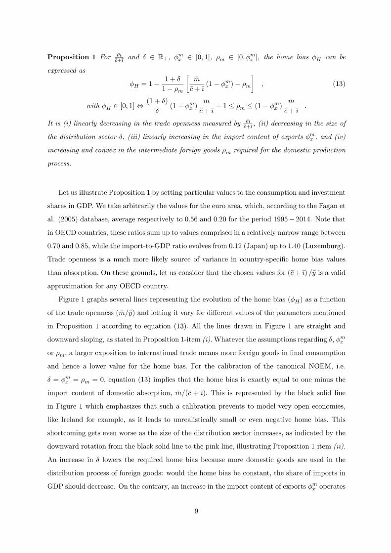
Proposition 1 For �m�c+�{ and � 2 R+, �mx 2 [0; 1], �m 2 [0; �mx ], the home bias �H can be
expressed as
�H = 1�1 + �
1� �m
��m
�c+�{(1� �mx )� �m
�; (13)
with �H 2 [0; 1],(1 + �)
�(1� �mx )
�m
�c+�{� 1 � �m � (1� �mx )
�m
�c+�{.
It is (i) linearly decreasing in the trade openness measured by �m�c+�{ , (ii) decreasing in the size of
the distribution sector �, (iii) linearly increasing in the import content of exports �mx , and (iv)
increasing and convex in the intermediate foreign goods �m required for the domestic production
process.
Let us illustrate Proposition 1 by setting particular values to the consumption and investment
shares in GDP. We take arbitrarily the values for the euro area, which, according to the Fagan et
al. (2005) database, average respectively to 0:56 and 0:20 for the period 1995� 2014. Note that
in OECD countries, these ratios sum up to values comprised in a relatively narrow range between
0:70 and 0:85, while the import-to-GDP ratio evolves from 0:12 (Japan) up to 1:40 (Luxemburg).
Trade openness is a much more likely source of variance in country-speci�c home bias values
than absorption. On these grounds, let us consider that the chosen values for (�c+�{) =�y is a valid
approximation for any OECD country.
Figure 1 graphs several lines representing the evolution of the home bias (�H) as a function
of the trade openness ( �m=�y) and letting it vary for di¤erent values of the parameters mentioned
in Proposition 1 according to equation (13). All the lines drawn in Figure 1 are straight and
downward sloping, as stated in Proposition 1-item (i). Whatever the assumptions regarding �, �mx
or �m, a larger exposition to international trade means more foreign goods in �nal consumption
and hence a lower value for the home bias. For the calibration of the canonical NOEM, i.e.
� = �mx = �m = 0, equation (13) implies that the home bias is exactly equal to one minus the
import content of domestic absorption, �m=(�c + �{). This is represented by the black solid line
in Figure 1 which emphasizes that such a calibration prevents to model very open economies,
like Ireland for example, as it leads to unrealistically small or even negative home bias. This
shortcoming gets even worse as the size of the distribution sector increases, as indicated by the
downward rotation from the black solid line to the pink line, illustrating Proposition 1-item (ii).
An increase in � lowers the required home bias because more domestic goods are used in the
distribution process of foreign goods: would the home bias be constant, the share of imports in
GDP should decrease. On the contrary, an increase in the import content of exports �mx operates
9
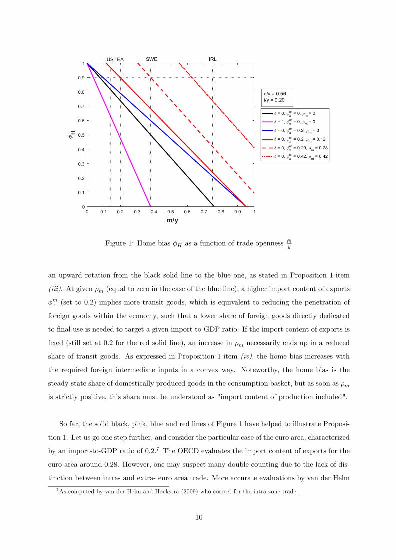
Figure 1: Home bias �H as a function of trade openness�m�y
an upward rotation from the black solid line to the blue one, as stated in Proposition 1-item
(iii). At given �m (equal to zero in the case of the blue line), a higher import content of exports
�mx (set to 0:2) implies more transit goods, which is equivalent to reducing the penetration of
foreign goods within the economy, such that a lower share of foreign goods directly dedicated
to �nal use is needed to target a given import-to-GDP ratio. If the import content of exports is
�xed (still set at 0:2 for the red solid line), an increase in �m necessarily ends up in a reduced
share of transit goods. As expressed in Proposition 1-item (iv), the home bias increases with
the required foreign intermediate inputs in a convex way. Noteworthy, the home bias is the
steady-state share of domestically produced goods in the consumption basket, but as soon as �m
is strictly positive, this share must be understood as "import content of production included".
So far, the solid black, pink, blue and red lines of Figure 1 have helped to illustrate Proposi-
tion 1. Let us go one step further, and consider the particular case of the euro area, characterized
by an import-to-GDP ratio of 0:2.7 The OECD evaluates the import content of exports for the
euro area around 0:28. However, one may suspect many double counting due to the lack of dis-
tinction between intra- and extra- euro area trade. More accurate evaluations by van der Helm
7As computed by van der Helm and Hoekstra (2009) who correct for the intra-zone trade.
10
and Hoekstra (2009) and by Amador et al. (2015) sets the import content of extra area exports
around 0:20. Figure 1 displays that, for �m=�y = 0:2, increasing �mx from 0 to 0:2 pushes the home
bias from 0:74 to 0:78 as long as �m = 0. For �m = 0:12, it raises up to 0:9 which is still on the
low side as it would imply, according to equation (8), that transit goods make 9 percent of euro
area exports, a most probably exaggerated value. Therefore, taking seriously empirical estimates
of the import content of exports into account allows to calibrate much higher home bias with all
the consequences it might have regarding, �rst, exchange rate volatility and the exchange rate
disconnect, as pointed by Wang (2010), and second, the pass-through to consumption prices, as
emphasized in the next sections of the present contribution.
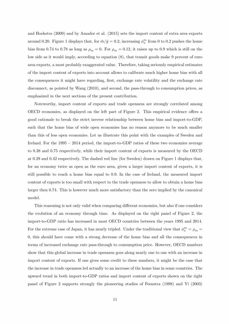
Noteworthy, import content of exports and trade openness are strongly correlated among
OECD economies, as displayed on the left part of Figure 2. This empirical evidence o¤ers a
good rationale to break the strict inverse relationship between home bias and import-to-GDP,
such that the home bias of wide open economies has no reason anymore to be much smaller
than this of less open economies. Let us illustrate this point with the examples of Sweden and
Ireland. For the 1995 � 2014 period, the import-to-GDP ratios of these two economies average
to 0:38 and 0:75 respectively, while their import content of exports is measured by the OECD
at 0:29 and 0:42 respectively. The dashed red line (for Sweden) drawn on Figure 1 displays that,
for an economy twice as open as the euro area, given a larger import content of exports, it is
still possible to reach a home bias equal to 0:9: In the case of Ireland, the measured import
content of exports is too small with respect to the trade openness to allow to obtain a home bias
larger then 0:74. This is however much more satisfactory than the zero implied by the canonical
model.
This reasoning is not only valid when comparing di¤erent economies, but also if one considers
the evolution of an economy through time. As displayed on the right panel of Figure 2, the
import-to-GDP ratio has increased in most OECD countries between the years 1995 and 2014.
For the extreme case of Japan, it has nearly tripled. Under the traditional view that �mx = �m =
0, this should have come with a strong decrease of the home bias and all the consequences in
terms of increased exchange rate pass-through to consumption price. However, OECD numbers
show that this global increase in trade openness goes along nearly one to one with an increase in
import content of exports. If one gives some credit to these numbers, it might be the case that
the increase in trade openness led actually to an increase of the home bias in some countries. The
upward trend in both import-to-GDP ratios and import content of exports shown on the right
panel of Figure 2 supports strongly the pioneering studies of Feenstra (1998) and Yi (2003)
11
Figure 2: Import content of exports �mx and trade openness�m�y in industrialized economies
on the rise of foreign value added in domestic production. It is clear from equation (2) that
this has direct implications for the respective weight of import and domestic production in the
consumption price index.
3.2 Composition of the consumption price index
According to equation (2), the price of consumption may be viewed as a weighted average of
the import price and the domestically produced goods price. Beside the reaction of each of these
prices to changes in the exchange rate, the steady-state proportion of the two homogenous goods
entering the composition of the �nal good is the key element of the pass-through to consumption
price. Log-linearized around steady-state, the price of the �nal good that is either consumed or
invested can be represented by
pt = �H ph;t +1� �H1 + �
(pf;t + �ph;t) ; (14)
where the second term is the retail price of the foreign good, i.e. after inclusion of domestic
distribution services.
12
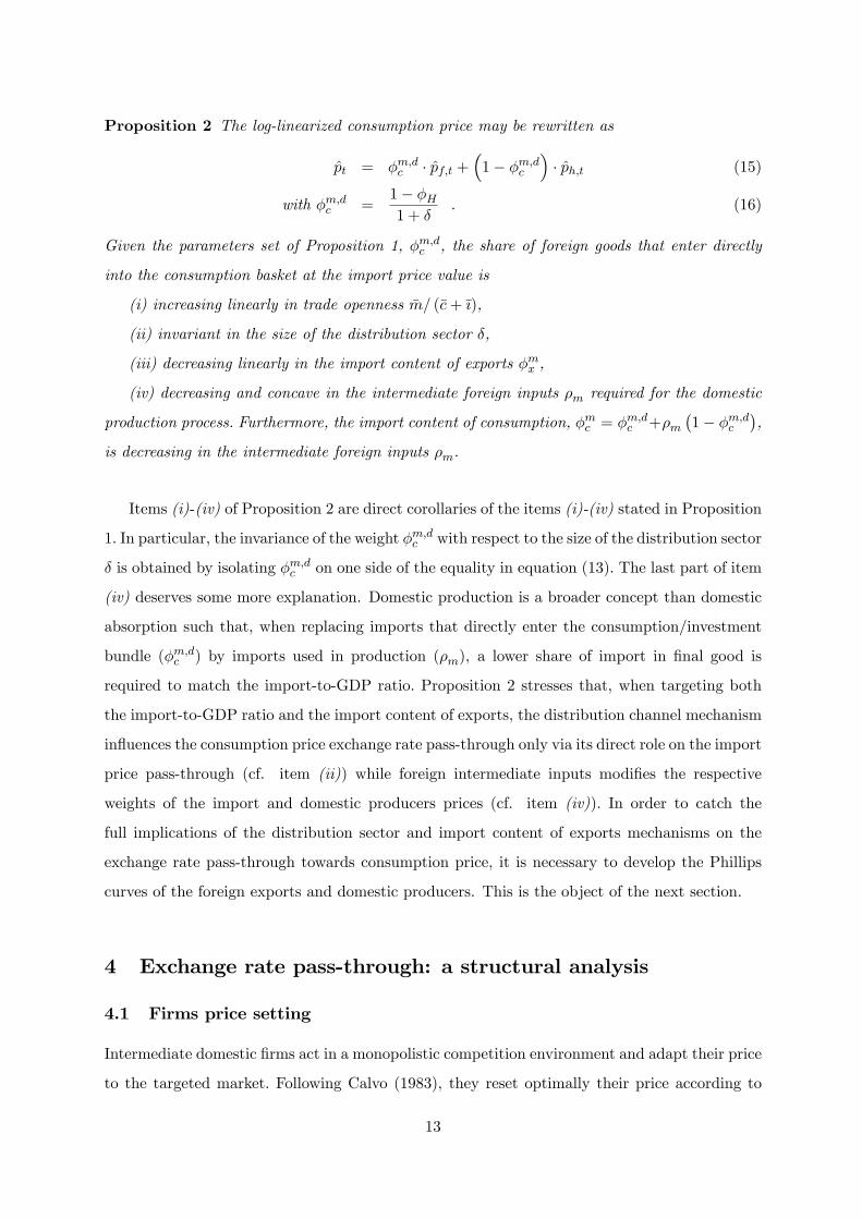
Proposition 2 The log-linearized consumption price may be rewritten as
pt = �m;dc � pf;t +�1� �m;dc
�� ph;t (15)
with �m;dc =1� �H1 + �
: (16)
Given the parameters set of Proposition 1, �m;dc , the share of foreign goods that enter directly
into the consumption basket at the import price value is
(i) increasing linearly in trade openness �m= (�c+�{),
(ii) invariant in the size of the distribution sector �,
(iii) decreasing linearly in the import content of exports �mx ,
(iv) decreasing and concave in the intermediate foreign inputs �m required for the domestic
production process. Furthermore, the import content of consumption, �mc = �m;dc +�m
�1� �m;dc
�,
is decreasing in the intermediate foreign inputs �m.
Items (i)-(iv) of Proposition 2 are direct corollaries of the items (i)-(iv) stated in Proposition
1. In particular, the invariance of the weight �m;dc with respect to the size of the distribution sector
� is obtained by isolating �m;dc on one side of the equality in equation (13). The last part of item
(iv) deserves some more explanation. Domestic production is a broader concept than domestic
absorption such that, when replacing imports that directly enter the consumption/investment
bundle (�m;dc ) by imports used in production (�m), a lower share of import in �nal good is
required to match the import-to-GDP ratio. Proposition 2 stresses that, when targeting both
the import-to-GDP ratio and the import content of exports, the distribution channel mechanism
in�uences the consumption price exchange rate pass-through only via its direct role on the import
price pass-through (cf. item (ii)) while foreign intermediate inputs modi�es the respective
weights of the import and domestic producers prices (cf. item (iv)). In order to catch the
full implications of the distribution sector and import content of exports mechanisms on the
exchange rate pass-through towards consumption price, it is necessary to develop the Phillips
curves of the foreign exports and domestic producers. This is the object of the next section.
4 Exchange rate pass-through: a structural analysis
4.1 Firms price setting
Intermediate domestic �rms act in a monopolistic competition environment and adapt their price
to the targeted market. Following Calvo (1983), they reset optimally their price according to
13
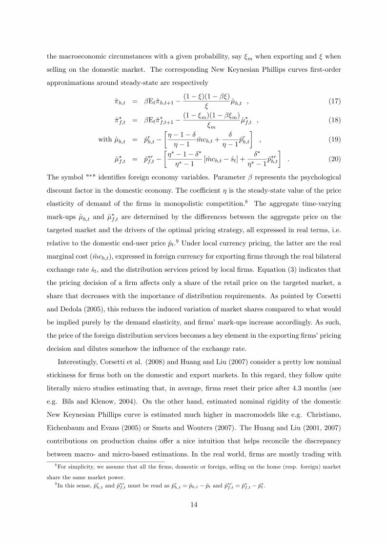
the macroeconomic circumstances with a given probability, say �m when exporting and � when
selling on the domestic market. The corresponding New Keynesian Phillips curves �rst-order
approximations around steady-state are respectively
�h;t = �Et�h;t+1 �(1� �)(1� ��)
��h;t , (17)
��f;t = �Et��f;t+1 �(1� �m)(1� ��m)
�m��f;t , (18)
with �h;t = prh;t ��� � 1� �� � 1 mch;t +
�
� � 1 prh;t
�, (19)
��f;t = p�rf;t ���� � 1� ��
�� � 1 [mch;t � st] +��
�� � 1 p�rh;t
�. (20)
The symbol "�" identi�es foreign economy variables. Parameter � represents the psychological
discount factor in the domestic economy. The coe¢ cient � is the steady-state value of the price
elasticity of demand of the �rms in monopolistic competition.8 The aggregate time-varying
mark-ups �h;t and ��f;t are determined by the di¤erences between the aggregate price on the
targeted market and the drivers of the optimal pricing strategy, all expressed in real terms, i.e.
relative to the domestic end-user price pt.9 Under local currency pricing, the latter are the real
marginal cost (mch;t), expressed in foreign currency for exporting �rms through the real bilateral
exchange rate st, and the distribution services priced by local �rms. Equation (3) indicates that
the pricing decision of a �rm a¤ects only a share of the retail price on the targeted market, a
share that decreases with the importance of distribution requirements. As pointed by Corsetti
and Dedola (2005), this reduces the induced variation of market shares compared to what would
be implied purely by the demand elasticity, and �rms�mark-ups increase accordingly. As such,
the price of the foreign distribution services becomes a key element in the exporting �rms�pricing
decision and dilutes somehow the in�uence of the exchange rate.
Interestingly, Corsetti et al. (2008) and Huang and Liu (2007) consider a pretty low nominal
stickiness for �rms both on the domestic and export markets. In this regard, they follow quite
literally micro studies estimating that, in average, �rms reset their price after 4:3 months (see
e.g. Bils and Klenow, 2004). On the other hand, estimated nominal rigidity of the domestic
New Keynesian Phillips curve is estimated much higher in macromodels like e.g. Christiano,
Eichenbaum and Evans (2005) or Smets and Wouters (2007). The Huang and Liu (2001, 2007)
contributions on production chains o¤er a nice intuition that helps reconcile the discrepancy
between macro- and micro-based estimations. In the real world, �rms are mostly trading with8For simplicity, we assume that all the �rms, domestic or foreign, selling on the home (resp. foreign) market
share the same market power.9 In this sense, prh;t and p
�rf;t must be read as p
rh;t = ph;t � pt and p�rf;t = p�f;t � p�t .
14
�rms, along a production process made of several intermediate steps and the price of the �nal
good is only set at the very last stage. The New Keynesian Phillips curve is built from the hor-
izontal integration of intermediate �rms acting in monopolistic competition and totally ignores
the vertical integration dimension. As a consequence, the dynamics of the observed macro price
series (e.g. the GDP de�ator) can only be reproduced through an estimated large degree of price
stickiness, which re�ects the modelling shortcut. However, when intermediate �rms export, be it
to foreign �rms or households, the cross-border price re�ects only one stage of production, such
that aggregate international price dynamics require much less nominal rigidity to be matched,
more in line with micro studies. In the absence of more information about intermediate prices,
the input-output structure and the average number of production steps, the empirical DSGE
literature estimates an overall large domestic producers�price rigidity that mimics the accumu-
lation of small intermediate price rigidities. In the rest of the paper we will rest on this simpli�ed
representation instead of following Huang and Liu (2001, 2007) in a more careful representation
of the production stages.10 In this logic, from then on we consider that �rms reoptimize their
price after 4:5 months when exporting (�m = 0:33) while they do it only after 3 quarters on the
domestic market (� = 0:75).
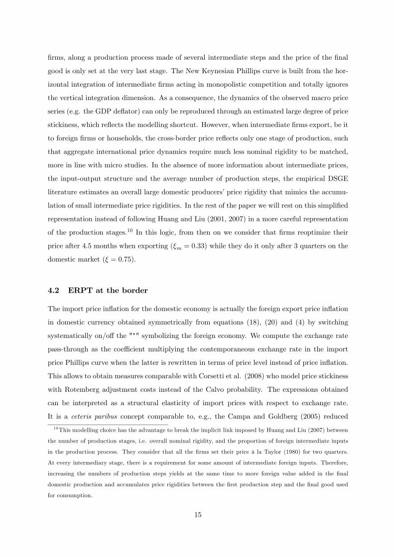
4.2 ERPT at the border
The import price in�ation for the domestic economy is actually the foreign export price in�ation
in domestic currency obtained symmetrically from equations (18), (20) and (4) by switching
systematically on/o¤ the "�" symbolizing the foreign economy. We compute the exchange rate
pass-through as the coe¢ cient multiplying the contemporaneous exchange rate in the import
price Phillips curve when the latter is rewritten in terms of price level instead of price in�ation.
This allows to obtain measures comparable with Corsetti et al. (2008) who model price stickiness
with Rotemberg adjustment costs instead of the Calvo probability. The expressions obtained
can be interpreted as a structural elasticity of import prices with respect to exchange rate.
It is a ceteris paribus concept comparable to, e.g., the Campa and Goldberg (2005) reduced
10This modelling choice has the advantage to break the implicit link imposed by Huang and Liu (2007) between
the number of production stages, i.e. overall nominal rigidity, and the proportion of foreign intermediate inputs
in the production process. They consider that all the �rms set their price à la Taylor (1980) for two quarters.
At every intermediary stage, there is a requirement for some amount of intermediate foreign inputs. Therefore,
increasing the numbers of production steps yields at the same time to more foreign value added in the �nal
domestic production and accumulates price rigidities between the �rst production step and the �nal good used
for consumption.
15
form pass-through estimates. In Proposition 3 below we operate a clear distinction between the
distribution sector and input trade assumptions for the sake of clarity.11 The fully general case
is developed in the technical appendix.
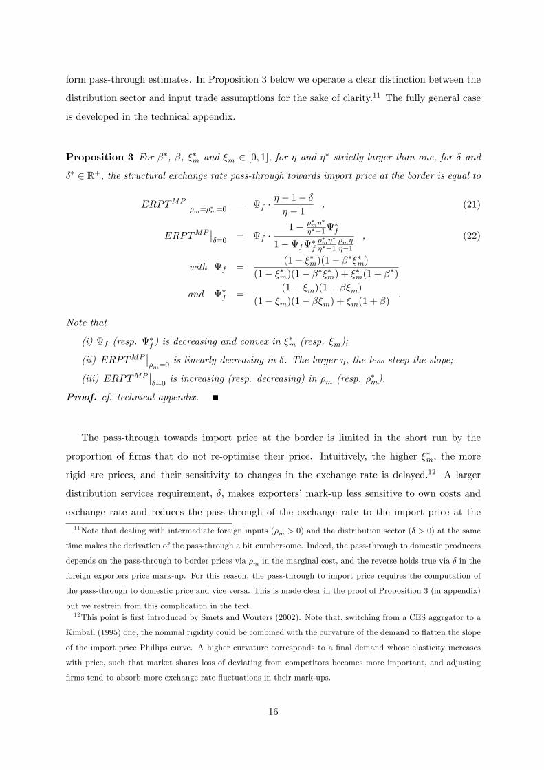
Proposition 3 For ��, �, ��m and �m 2 [0; 1], for � and �� strictly larger than one, for � and
�� 2 R+, the structural exchange rate pass-through towards import price at the border is equal to
ERPTMP���m=�
�m=0
= f �� � 1� �� � 1 , (21)
ERPTMP���=0
= f �1� ��m�
�
���1�f
1�f�f��m�
�
���1�m���1
, (22)
with f =(1� ��m)(1� ����m)
(1� ��m)(1� ����m) + ��m(1 + ��)
and �f =(1� �m)(1� ��m)
(1� �m)(1� ��m) + �m(1 + �).
Note that
(i) f (resp. �f ) is decreasing and convex in ��m (resp. �m);
(ii) ERPTMP���m=0
is linearly decreasing in �. The larger �, the less steep the slope;
(iii) ERPTMP���=0
is increasing (resp. decreasing) in �m (resp. ��m).
Proof. cf. technical appendix.
The pass-through towards import price at the border is limited in the short run by the
proportion of �rms that do not re-optimise their price. Intuitively, the higher ��m, the more
rigid are prices, and their sensitivity to changes in the exchange rate is delayed.12 A larger
distribution services requirement, �, makes exporters�mark-up less sensitive to own costs and
exchange rate and reduces the pass-through of the exchange rate to the import price at the
11Note that dealing with intermediate foreign inputs (�m > 0) and the distribution sector (� > 0) at the same
time makes the derivation of the pass-through a bit cumbersome. Indeed, the pass-through to domestic producers
depends on the pass-through to border prices via �m in the marginal cost, and the reverse holds true via � in the
foreign exporters price mark-up. For this reason, the pass-through to import price requires the computation of
the pass-through to domestic price and vice versa. This is made clear in the proof of Proposition 3 (in appendix)
but we restrein from this complication in the text.12This point is �rst introduced by Smets and Wouters (2002). Note that, switching from a CES aggrgator to a
Kimball (1995) one, the nominal rigidity could be combined with the curvature of the demand to �atten the slope
of the import price Phillips curve. A higher curvature corresponds to a �nal demand whose elasticity increases
with price, such that market shares loss of deviating from competitors becomes more important, and adjusting
�rms tend to absorb more exchange rate �uctuations in their mark-ups.
16
border. As highlighted by Corsetti and Dedola (2005), the lower the demand elasticity, the
stronger the potential of the distribution margin to decrease ERPTMP .
Interestingly, both the distribution channel and the input trade mechanisms allow to obtain
a pass-through to import prices at the border that is incomplete under �exible prices, i.e. for
f = �f = 1. For the distribution services, the reason for the path-through incompleteness
lies in the increased mark-up of the foreign exporting �rms, as reported supra. For the input
trade, the explanation comes from the marginal cost of the foreign exporting �rms, that include
a share ��m��=(�� � 1) of home produced goods. For the latter share, the exchange rate e¤ect
on the import price cancels out, as highlighted by Georgiadis, Gräb and Khalil (2018). This
is the economic intuition behind items (iii) of Proposition 3 that establishes that the pass-
through to import price decreases with the integration of home produced goods in the foreign
production process. On the contrary, if the home economy uses more foreign intermediate inputs,
the exchange rate is partially cancelled out back and forth, and pass-through increases.
4.3 ERPT towards domestic production price
In models that do not consider intermediate foreign inputs in the production process, the relative
price of currencies does not a¤ect the domestic price Phillips curve. However, given the inter-
nationalization of the production process brie�y documented in Section 3, the share of foreign
value-added contained into a domestic �nal good is certainly not negligible. In the production
process with �m > 0, the exchange rate a¤ects the marginal cost of domestic producers via its
role in the determination of import prices. The structural pass-through to domestic producers
prices, ERPTDP , is equal to the coe¢ cient multiplying the exchange rate in equation (17) when
the latter is rewritten in terms of price level rather than in�ation.
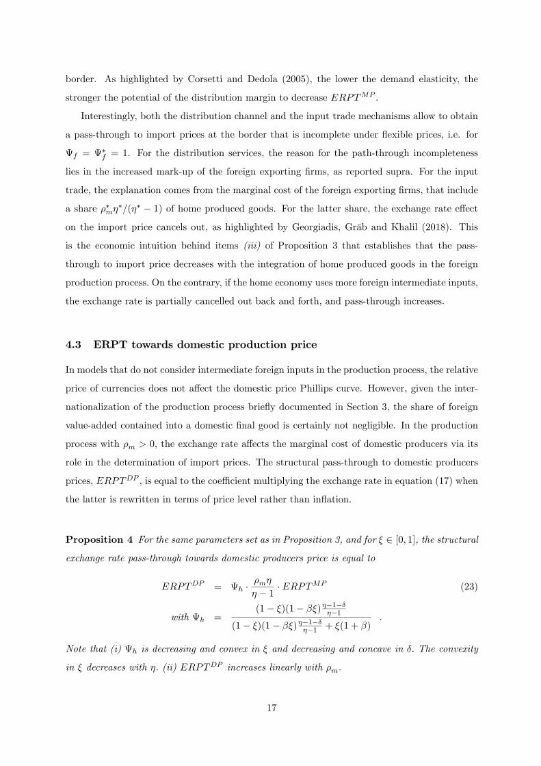
Proposition 4 For the same parameters set as in Proposition 3, and for � 2 [0; 1], the structural
exchange rate pass-through towards domestic producers price is equal to
ERPTDP = h ��m�
� � 1 � ERPTMP (23)
with h =(1� �)(1� ��)��1����1
(1� �)(1� ��)��1����1 + �(1 + �).
Note that (i) h is decreasing and convex in � and decreasing and concave in �: The convexity
in � decreases with �. (ii) ERPTDP increases linearly with �m.
17

Expression (23) makes clear that the pass-through of the exchange rate to the domestic
producers�price is limited twice: �rst via the combination of nominal and real rigidities that
apply to the price dynamics of imported intermediate goods, speci�ed supra, and second, via
the combination of nominal and real rigidities that drive the price dynamics of domestically
produced goods.
4.4 ERPT towards the consumption price index
All the results gathered at this stage allow to establish some conclusions regarding the trans-
mission of the relative value of the domestic currency to the consumption de�ator. They are
formally stated in the following Corollaries.
Corollaries of Propositions 2, 3 and 4
- C0: equation (15) may be turned into
ERPTCP = �m;dc ERPTMP +�1� �m;dc
�ERPTDP ; (24)
- C1: The parameters a¤ecting the slope of the import price Phillips curve, i.e. ��m, �, and
�, make it possible to match any ERPTMP . International trade in intermediate inputs
may also help, through ��m, though his potential is more limited in this respect and is
reduced further by �m (cf. Proposition 3);
- C2: for �m = 0 and �mx = 0, the relationship between ERPT
CP and ERPTMP is strictly
linear in �m= (�c+�{), which renders extremely unlikely to simultaneously match the two pass-
throughs, notably for large trade openness. Neither the slope of the import price Phillips
curve nor the distribution channel are able to break this linear relationship;
- C3: Allowing �mx > 0 o¤ers the required �exibility to circumvent C2 by decreasing �m;dc .
However, as long as �m = 0, it may induce an unrealistically large degree of import content
of export under the form of transit goods;
- C4: Allowing �m > 0 rebalances equation (24) away from the import price pass-through
towards the domestic production price pass-through, which is much smaller (cf. e.g. equa-
tion (23)). At given �mx > 0, a marginal increase of �m is much more e¢ cient to decrease
�m;dc than a marginal increase in �mx (cf. Proposition 2-items (iii) and (iv)), reducing the
need for large import content of exports in general and for transit goods in particular.
18
According to Corollaries C3 and C4, it is possible for a more open economy to face the same
consumption price structural pass-through as this of a less open economy. The intuition is exactly
similar to this developed supra for the home bias: the initial handicap of a large trade openness
can be circumvented by more import content of exports, which in OECD economies are indeed
observed to be strongly positively correlated with trade openness. Furthermore, the required
import content of exports may be relatively reduced if it is mainly composed of intermediate
foreign inputs rather than of transit goods.
4.5 A numerical illustration
In order to illustrate Corollaries C1-C4, let us give speci�c values to the most obvious ratios and
coe¢ cients to help assess numerically the implication of the reviewed pass-through attenuating
mechanisms for the euro area. As in Figure 1 we pose �c=�y = 0:56 and �{=�y = 0:20. The import-to-
GDP ratio for extra trade has been evaluated by van der Helm and Hoekstra (2009) at 0:20. The
parameters appearing in the Phillips curve equations are calibrated at fairly standard values:
the discount rate � is set equal to 0:99 and the elasticity of substitution between intermediate
goods on markets in monopolistic competition is set equal to 4:5.
Illustrating Corollaries C1-C4: �exible import prices Figure 3 depicts how three of
the mechanisms discussed so far a¤ect the pass-through to consumption price and via which
channel under perfectly �exible import prices (��m = 0) for an economy calibrated for the euro
area. The upper-left panel illustrates Corollary 2: as the size of the distribution sector increases,
the importance of the exchange rate in the foreign exporters pricing decision (cf. equations (20)
and (21)) declines, reducing the pass-through towards import price. The size of the distribution
sector does not a¤ect �m;dc , the weight of import price in the consumption price index, such that
the decrease in the pass-through to import price is transmitted directly to the consumption price
with a proportion factor equal to �m;dc , as emphasized by Corollary C2. The distribution margin,
i.e. �=(1 + �), has to increases up to 64% in order to reduce both ERPTMP and ERPTCP by
�fty percent.
Corollary C3 is put into perspective on the upper-right panel of Figure 3. The larger the
share of transit goods in the exports, the lower the steady-state share �m;dc of imports entering
the �nal good bundle at their border price, and a lower pass-through to consumption price can
be obtained with a given and unchanged pass-through to import price. In order to halve the
19
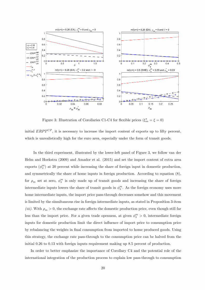
Figure 3: Illustration of Corollaries C1-C4 for �exible prices (��m = � = 0)
initial ERPTCP , it is necessary to increase the import content of exports up to �fty percent,
which is unrealistically high for the euro area, especially under the form of transit goods.
In the third experiment, illustrated by the lower-left panel of Figure 3, we follow van der
Helm and Hoekstra (2009) and Amador et al. (2015) and set the import content of extra area
exports (�mx ) at 20 percent while increasing the share of foreign input in domestic production,
and symmetrically the share of home inputs in foreign production. According to equation (8),
for �m set at zero, �mx is only made up of transit goods and increasing the share of foreign
intermediate inputs lowers the share of transit goods in �mx . As the foreign economy uses more
home intermediate inputs, the import price pass-through decreases somehow and this movement
is limited by the simultaneous rise in foreign intermediate inputs, as stated in Proposition 3-item
(iii). With �m > 0, the exchange rate a¤ects the domestic production price, even though still far
less than the import price. For a given trade openness, at given �mx > 0, intermediate foreign
inputs for domestic production limit the direct in�uence of import price to consumption price
by rebalancing the weights in �nal consumption from imported to home produced goods. Using
this strategy, the exchange rate pass-through to the consumption price can be halved from the
initial 0:26 to 0:13 with foreign inputs requirement making up 8:5 percent of production.
In order to better emphasize the importance of Corollary C4 and the potential role of the
international integration of the production process to explain low pass-through to consumption
20
prices, let us consider an economy for which trade is two times more important than for the euro
area, as Sweden for example (cf. Figure 1). According to Figure 1, for � = �mx = �m = 0, the
pass-through to consumption price would be equal to a huge 0:50. However, the OECD computes
that Swedish import content of exports amounts to 0:29 (average 1995-2014): As displayed on
the lower right panel of Figure 3, for �m = 0, this corresponds still to an unrealistically high
pass-through to consumption of 0:32. Rising foreign intermediate inputs up to the maximum,
i.e. 29 percent of the domestic production, the pass-through to consumption price decreases to
0:17, slightly above the targeted value in the three previous experiments.13 The latter exercise
con�rms the intuition raised earlier that the nominal side of a quite open economy is not neces-
sarily much more a¤ected by exchange rate �uctuations than this of a more closed one. Instead,
the e¤ect of exchange rate �uctuations on domestic prices strongly depends on the extent to
which the economy is integrated into global value chains, and whether that integration is lim-
ited to exports or extends to total domestic production. It is straightforward to carry on this
illustration to relationship between import price nominal stickiness and pass-throughs.
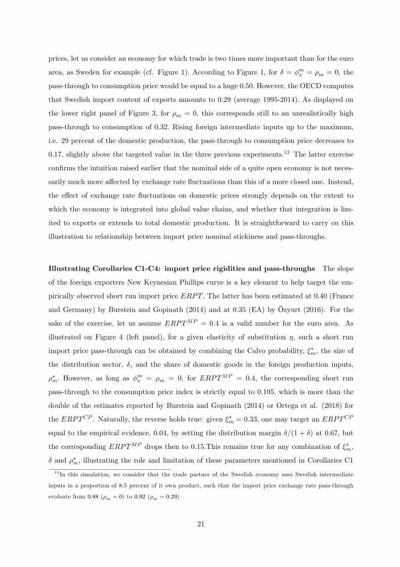
Illustrating Corollaries C1-C4: import price rigidities and pass-throughs The slope
of the foreign exporters New Keynesian Phillips curve is a key element to help target the em-
pirically observed short run import price ERPT . The latter has been estimated at 0:40 (France
and Germany) by Burstein and Gopinath (2014) and at 0:35 (EA) by Özyurt (2016). For the
sake of the exercise, let us assume ERPTMP = 0:4 is a valid number for the euro area. As
illustrated on Figure 4 (left panel), for a given elasticity of substitution �, such a short run
import price pass-through can be obtained by combining the Calvo probability, ��m, the size of
the distribution sector, �, and the share of domestic goods in the foreign production inputs,
��m: However, as long as �mx = �m = 0, for ERPTMP = 0:4, the corresponding short run
pass-through to the consumption price index is strictly equal to 0:105, which is more than the
double of the estimates reported by Burstein and Gopinath (2014) or Ortega et al. (2018) for
the ERPTCP . Naturally, the reverse holds true: given ��m = 0:33, one may target an ERPTCP
equal to the empirical evidence, 0:04, by setting the distribution margin �=(1 + �) at 0:67, but
the corresponding ERPTMP drops then to 0:15.This remains true for any combination of ��m,
� and ��m, illustrating the role and limitation of these parameters mentioned in Corollaries C1
13 In this simulation, we consider that the trade partner of the Swedish economy uses Swedish intermediate
inputs in a proportion of 8:5 percent of it own product, such that the import price exchange rate pass-through
evoluate from 0:88 (�m = 0) to 0:92 (�m = 0:29)
21
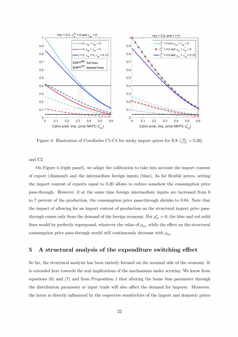
Figure 4: Illustration of Corollaries C1-C4 for sticky import prices for EA ( �m�c+�{ = 0:26)
and C2.
On Figure 4 (right panel), we adapt the calibration to take into account the import content
of export (diamond) and the intermediate foreign inputs (blue). As for �exible prices, setting
the import content of exports equal to 0:20 allows to reduce somehow the consumption price
pass-through. However, if at the same time foreign intermediate inputs are increased from 0
to 7 percent of the production, the consumption price pass-through shrinks to 0:04. Note that
the impact of allowing for an import content of production on the structural import price pass-
through comes only from the demand of the foreign economy. For ��m = 0, the blue and red solid
lines would be perfectly superposed, whatever the value of �m, while the e¤ect on the structural
consumption price pass-through would still continuously decrease with �m.
5 A structural analysis of the expenditure switching e¤ect
So far, the structural analysis has been entirely focused on the nominal side of the economy. It
is extended here towards the real implications of the mechanisms under scrutiny. We know from
equations (6) and (7) and from Proposition 1 that altering the home bias parameter through
the distribution parameter or input trade will also a¤ect the demand for imports. Moreover,
the latter is directly in�uenced by the respective sensitivities of the import and domestic prices
22
to exchange rate �uctuations. In this sense, any mechanism able to mitigate the pass-through
to the import price, producers�price or consumer price will not only a¤ect the nominal side of
the economy, but has real consequences by altering the channels and the determinants of the
demand for imports. This is made clear in the following proposition, illustrated by Figure 5
below.
Proposition 5 Substituting for (12) into equation (11) and loglinearizing, the real imports equa-
tion of the home economy may be written as
mt = (��) 1 (pf;t � ph;t) + (��m) 2 (pf;t � mch;t)
+3
�c
c+ ict +
i
c+ i{t
�+ xt�
mx (25)
with 1 =�c+�{
�m
(1� �H)(1 + �)2
[�H (1� �m)� �m�] ; 2 = 1�1� �H1 + �
�c+�{
�m� �
mx � �m1� �m
;
3 =�c+�{
�m
1� �H (1� �m) + �m�1 + �
.
According to this expression, a weaker slope of the import price Phillips curve obtained via
parameters ��m, � and ��m limits structurally the expenditure switching e¤ect linked to changes
in the import price relative to the domestic producers� price. This is also true for the import
content of exports, �mx , and the foreign value added in production, �m, as long as �m remains
contained with respect to �. Finally, as long as �mx = �m = 0, the distribution sector leaves the
elasticity of real imports to absorption (3) unchanged at 1, while this elasticity decreases in �mx
and �m.
Proof. Concerning the relative prices, Propositions 3 establishes that parameters ��m, � and
��m driving the slope of the import price Phillips curve either delay or limit the transmission
of relative currency �uctuations towards import price. Furthermore, both distribution services
and input trade establish a link between border import price and domestic producers�price that
reduces the price gap: the �rst one operates via the import price mark-up (cf. equation (20))
and the second one via the domestic producers�marginal cost (cf. equation (4)). Beside this,
the coe¢ cients of the relative prices in equation (25) also matter and one observes that
(i) 1 is decreasing and convex in � and 2 is invariant in �;
(ii) 1 is decreasing and concave in �mx and 2 is invariant in �mx ;
(iii) 1 is decreasing and concave in �m and 2 is increasing and convex in �m, such that,
for � su¢ ciently large compared to �m, the �rst one dominates.
23
In the absence of distribution services and input trade, the elasticity of imports to the
relative price of imports is simply equal to the Armington trade elasticity multiplied by the non-
imported share of absorption.14 From equation (3), we see that the requirement of distribution
services has the natural consequence of decreasing the volume of trade that is a¤ected by the
price competition between �nal home and foreign goods. From Proposition 2-items (iii)-(iv),
we know that the same holds true for the import content of exports and production: higher �mx
and �m involve a decrease of �m;dc = (1� �H)=(1 + �), i.e. the share of the border import price
in the consumption price index, which is a¤ected by the expenditure switching e¤ect linked
to variations in the relative price. However, once input trade is introduced, the demand of
domestic producers for imports depends also on the relative price of imports with respect to
the cost of the domestic production factors, via 2. This channel counterbalances the decrease
of �m;dc = (1� �H)=(1 + �) and reinforces the expenditure switching e¤ect in proportion of the
corresponding trade elasticity, �m. Finally, note that the elasticity between real imports and
absorption remains unchanged and equal to one as long as the import content of exports is set
to zero. Once the latter becomes positive, the motives behind imports are broadened to transit
and production purposes and the sensitivity of imports to private aggregate demand decreases.
Proposition 5 is illustrated on Figure 5 which produces a numerical example for the calibra-
tion used so far, i.e. �m=(�c +�{) = 0:26, corresponding to the euro area: The left panel displays
the strong e¤ect of an increase of the distribution margin �=(1 + �) from 0 to 67 percent on
the coe¢ cient of the relative price in the import demand, abstracting from the trade elasticity:
coe¢ cient 1 drops from 0:74 to 0:07. On the second panel, one observes that transit goods
have a lower potential in mitigating the expenditure switching e¤ect, but they a¤ect the im-
port/absorption relationship as synthesized by 3. Finally, the third panel illustrates the e¤ect
of foreign intermediate inputs in production on the expenditure switching e¤ect. In the case of
a Leontief production technology, the potential of this mechanism to reduce the expenditure
switching e¤ect is as important as this of the distribution sector. However, it is opposed by a
strong force in opposite direction once departing from the pure complementarity assumption.
We conclude from this that, assuming perfect complementarity between home and foreign inputs
in the domestic production process, input trade and distribution services have a rather similar
potential to reduce the expenditure switching e¤ect, but the sensitivity to absorption is reduced
in the former mechanism compared to the latter.
14One easily compute that 1(� = �mx = �m = 0) = �H = 1� �m�c+�{.
24
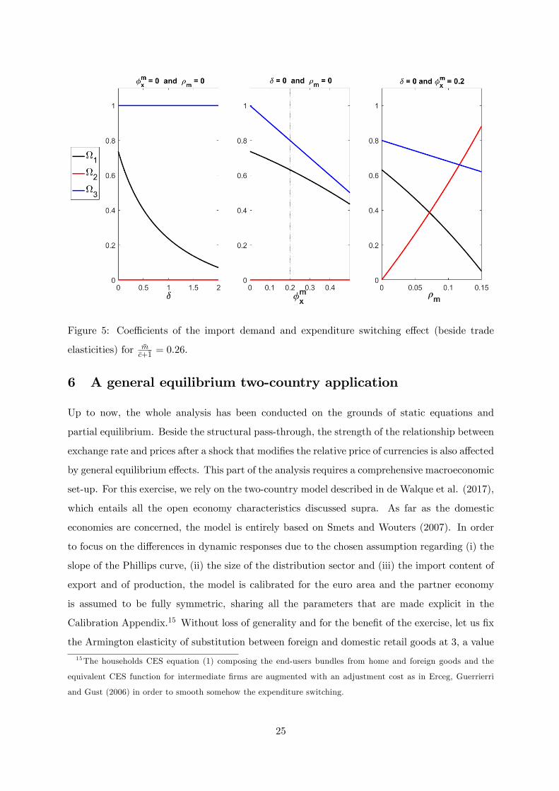
Figure 5: Coe¢ cients of the import demand and expenditure switching e¤ect (beside trade
elasticities) for �m�c+�1
= 0:26:
6 A general equilibrium two-country application
Up to now, the whole analysis has been conducted on the grounds of static equations and
partial equilibrium. Beside the structural pass-through, the strength of the relationship between
exchange rate and prices after a shock that modi�es the relative price of currencies is also a¤ected
by general equilibrium e¤ects. This part of the analysis requires a comprehensive macroeconomic
set-up. For this exercise, we rely on the two-country model described in de Walque et al. (2017),
which entails all the open economy characteristics discussed supra. As far as the domestic
economies are concerned, the model is entirely based on Smets and Wouters (2007). In order
to focus on the di¤erences in dynamic responses due to the chosen assumption regarding (i) the
slope of the Phillips curve, (ii) the size of the distribution sector and (iii) the import content of
export and of production, the model is calibrated for the euro area and the partner economy
is assumed to be fully symmetric, sharing all the parameters that are made explicit in the
Calibration Appendix.15 Without loss of generality and for the bene�t of the exercise, let us �x
the Armington elasticity of substitution between foreign and domestic retail goods at 3, a value
15The households CES equation (1) composing the end-users bundles from home and foreign goods and the
equivalent CES function for intermediate �rms are augmented with an adjustment cost as in Erceg, Guerrierri
and Gust (2006) in order to smooth somehow the expenditure switching.
25
close to the one estimated by de Walque et al. (2017) for the period 1970Q1-2014Q4.16 The
log-linearized uncovered interest rate parity condition is given by
St = EtSt+1 + r�t � rt � �nnfat + "st , (26)
where St represents the nominal exchange rate in relative deviation from steady-state, r�t is the
absolute percentage variation of the foreign short-term nominal interest, and rt its home coun-
terpart. nfat is the percentage deviation with respect to steady-state of the domestic holdings of
net foreign assets, ensuring the solution stability. Finally, "st is an auto-regressive process of order
one, capturing exogenous variations in international �nancial market conditions.17 Beside "st ,
any shock in the domestic or the foreign economy that a¤ects one of the interest rates through
the reaction of the monetary policy, will modify the bilateral exchange rate. The monetary
policy is represented by a Taylor rule based on Smets and Wouters (2007):
rt = �rrt�1 + (1� �r)����c;t + �ygy
gt
�+ ��yg
�ygt � y
gt�1�+ "rt
where ygt represents the di¤erential between real domestic value added and potential domestic
value added measured as the GDP prevailing in a counterfactual economy with �exible prices
and wages.
The strength of the relationship between prices and the exchange rate can then be assessed
by
PERRil;t =
Ptj=0 �
il;jPt
j=0�Sij
; l 2 ff; h; cg (27)
where PERR is the acronym for Price to Exchange Rate Ratio, a measure introduced in the
exchange rate pass-through literature by Shambaugh (2008). Index l associated with in�ation
speci�es for which speci�c price - import, f , domestic producers, h, or consumer, c - the rela-
tionship is computed. Index i on each variable stresses that the strength of this co-movement is
actually shock dependent.
16Such a value is admittedly high compared to the trade elasticities usually found in the NOEM literature,
that are more around unity. However, it is not the value of the elasticity per se which is of interest, but how its
implications in terms of expenditure switching e¤ect are modi�ed by the di¤erent variants examined. A careful
analysis of the interaction between the trade elasticities and the two mechanisms studied here - input trade and
distribution - is one of the topics of an estimated sequel of the present paper.17Note that in this two-country symmetric set-up, this term is the only potential source of assymetry. We limit
it by calibrating �n to 10�5, a fairly low value that still ensure stability and robustenss of the simulations.
26
6.1 Dynamic responses to an unexpected depreciation
As the �rst objective of the present contribution is to deal with the exchange rate pass-through,
it seems natural to start the exercise with the study of the macroeconomic dynamics after an
unexpected depreciation of the home currency. The persistence of the UIP autoregressive process
"st is set equal to 0:80 and the size of the shock is chosen to generate an on impact depreciation
by one percent for the benchmark NOEM with � = �mx = �m = 0. The UIP shock has the
distinctive feature to be common to both economies and the full symmetry assumption adopted
supra implies that the reaction of the foreign economy exactly mirrors this of the home economy.
Let us observe and discuss the implications of departing from the benchmark model by playing
with (i) the slope of the import price Phillips curve, (ii) the size of the distribution sector and
(iii) input trade in order to target a structural pass-through to consumption price, ERPTCP , of
0:04. The corresponding parametrizations can readily be inferred from Figure 4 and the impulse
response functions obtained for the four variants considered are displayed on Figure 6.
6.1.1 Varying the slope of the import price NKPC
In the benchmark simulation (full black line), the slope of the import price Phillips curve is
determined solely by the Calvo probability of not re-optimizing, ��m, which is set to 0:33 such
that ERPTMP = 0:4 and ERPTCP = 0:105 (cf. Figure 4). The admittedly high trade elasticity
implies that the di¤erence in import and producers�prices in the home (resp. foreign) economy
triggers a strong reallocation of the global demand away (resp. towards) from foreign (resp.
home) goods. The surge in foreign demand for home produced goods more than compensates
the negative e¤ect of the imported in�ation on the home private absorption and pushes domestic
producers price upwards.
The full red line on Figure 6 displays the consequences of increasing the Calvo probabil-
ity to 0:56, which corresponds to an average price duration of 7 months instead of the initial
4.5. This has the consequence of drawing the structural pass-through downwards such that
ERPTMP = 0:15 and ERPTCP = 0:04. The nominal rigidity determines the hump-shaped
pro�le of the import price reaction which is directly transmitted to the consumption price. As
the slope of the import price Phillips curve �attens, the price di¤erential is reduced, thereby
limiting the expenditure switching e¤ect and the general equilibrium forces that generate in�a-
tion in the domestic producers�price. Given the weight of the latter (1 � �m;dc = 0:74) in the
consumption price index, this e¢ ciently supplements the delayed reaction of import price to
27
limit the transmission of exchange rate to consumption price.
As already stated in the related literature, the low pass-through to consumption price ob-
tained via the nominal stickiness in the import price Phillips curve is reached at the cost of
unrealistically low transmission of the exchange rate to import price in the short run. Said dif-
ferently, the initial reduction of the PERRsc;t ratio the �rst four quarters after the shock is the
outcome of the modi�cation of the pro�le of the PERRsf;t ratio. Therefore, the lack of �exibility
found in the case of the ERPT disconnect in Section 4 also re�ects here in the PERRs. This is
one major argument on which Corsetti at al. (2008) grounds to introduce a distribution sector
à la Burstein et al. (2003) in NOEM, in the hope of circumventing this identi�ed weakness. Let
us observe in a dynamic framework whether their intuition is indeed veri�ed.
6.1.2 Varying the need for domestic distribution services
Setting the foreign exporters�Calvo probability back to its initial value of 0:33, a structural
pass-through to consumption price of 0:04 coherent with empirical �ndings can be obtained by
considering a distribution margin �=(1 + �) equal to 0:67. As stated in Propositions 3 and 5,
at given trade openness, the size of the distribution sector alters the import demand. First, in
the foreign exporters�mark-up, it partially substitutes the own marginal cost and exchange rate
for the price of home distribution services, reducing the relative price gap between foreign and
home goods. Second, it attenuates the import sensitivity to this relative price, 1. The latter
is reduced by a factor ten compared to the benchmark (cf. Figure 5, left panel). Both elements
contribute to limit sharply the expenditure switching e¤ect. The impulse responses to a UIP
shock (full blue lines) computed on Figure 6 for the net trade and real GDP displays how the
mechanism wipes the growth prospect of a depreciation o¤.
For the given UIP shock, the real and nominal consequences of increasing � reduce the
endogenous reaction of the monetary policy, which pushes upwards the exchange rate. It also
enhances the foreign marginal cost, mirror of the home one, but dampens the reaction of the
domestic producers�price, and thus of domestic distribution prices. As the distribution margin
increases, this second element opposes and dominates the �rst one within the foreign exporting
�rms�mark-up.18 Given the parametrization choice and according to equation (20), the domestic
producers�price represents now �=(��1) = 57 percent of the foreign exporters�mark-up, and the18The di¤erential beteen the nominal stickiness in the import price and domestic producers price Phillips curve
plays an important role here, through the increased persistence associated to the home real marginal cost compared
to this associated with the foreign one.
28

import price reaction is strongly tuned down with respect to the benchmark (black full line) or
the higher import price Calvo (red line). This also implies that the dynamics of the consumption
price are more in�uenced by the domestic producers�price which accounts now for 80 percent of
it, computed as (1� �m;dc ) + �m;dc f���1 . Finally, the producers�price itself is strongly a¤ected
by the depressed foreign demand for home goods relative to the benchmark NOEM (black full
line).
Figure 6: Impulse responses to a UIP shock
Domestic distribution services are more e¢ cient than nominal stickiness to obtain a low
transmission of exchange rate �uctuations to consumption price. However Figures 6 illustrates
29
that the general equilibrium mechanisms at work do not strongly modify the conclusion stated
in Corollary C2 for a static environment: in both cases, the lower transmission of exchange rate
towards consumption price is reached by reducing the (empirically observed large) transmission
to import price. This is particularly well illustrated by the Shambaugh (2008) PERRsf;t and
PERRsc;t indicators. Reducing the gap between import and consumption prices at the retail
level either via a �attening of the import price Phillips curve only (full red line) or through
distribution services (full blue line) pushes down the PERR concept of consumption price pass-
through but at the cost of an ab initio strong deformation of the exchange rate-import price
relationship. As such, when estimating an open economy model, the Calvo parameter will help
capture the import price dynamics, the assumption of a distribution sector may supplement the
trade elasticity � in dealing with some features of the observed real series, but none of them
o¤ers a credible potential to reconcile the high exchange rate/import price connectedness with
the low transmission of currency price to consumption price. This conclusion is not astonishing
as the very essence of both mechanisms is to bring the import price dynamics closer to the
producers�price one, reducing the relative price gap. This is obviously not the case for the trade
input extension (cf. Corollaries C3 and C4).
6.1.3 Varying the import content of exports and of production
Transit goods and intermediate foreign inputs operate directly by rebalancing the respective
weights of import price at the border and domestic prices within the end-user price index as
highlighted in Proposition 2. Integrating import content of exports under the form of transit
goods only by setting �mx = 0:2 (euro area calibration) and �m = 0 would be equivalent to
reducing the actual trade openness of the economies. As for the Calvo and the distribution sector,
Figure 6 (dashed black line) focuses on the case where ERPTCP = 0:04, which is obtained for an
import content of production, �m, set equal to 10 percent. It considers perfect complementarity
between home and foreign inputs in the production process (�m = 0 in equation (12)), such
that the expenditure switching e¤ect is fully driven by 1, which is reduced to 0:27 according
to Figure 5.
The larger �m, the stronger the domestic marginal cost reaction to the exchange rate, which
is translated into higher domestic producers�price. Concurrently, for the chosen calibration, the
respective weights of import price and domestic price into the consumption price index (i.e. �m;dc
and 1��m;dc ) are reset to 0:09�0:91 instead of 0:26�0:74 for the previous exercises displayed on
Figure 6. Indeed, a share �m=(1� �m) of imports enters the consumption price index indirectly,
30

via a �at domestic price Phillips curve (� = 0:75), instead than directly, through a much steeper
import price Phillips curve (��m = 0:33). Depreciation becomes less in�ationary and the real
private home (resp. foreign) demand reacts less negatively (resp. positively). For the Leontief
production function studied here, the foreign �rms�demand for home produced intermediate
inputs does not increase with the depreciation of the domestic currency. Furthermore, the
share of foreign goods concerned by the home households�decision regarding their �nal goods
composition is nearly divided by three compared to the benchmark case (black line) such that
the reaction of the real variables is strongly mitigated, as observed above for the distribution
services. At an horizon of four years, the import price to exchange rate relationship PERRsf;t
is left relatively unchanged with respect to the benchmark, while the relative sensitivity of the
consumption price, PERRsc;t, is strongly reduced, extending the validity of Corollaries C3 and
C4 to the case of a general equilibrium analysis.
6.1.4 On the role of foreign/domestic inputs substitutability (�m)
Let us now depart from the Leontief technology driving the mix of home/foreign intermediate
inputs for the domestic �rms in monopolistic competition and allow them to react more �exibly
to changes in the imports relative price. We �x the trade elasticity �m = � = 3 such that �rms
adopt the same behavior as the households regarding relative prices. A priori, one could think
that such a �exibility should help reduce further the transmission of exchange rates to domestic
prices. In the words of Campa and Goldberg (2010): "Calibrated price e¤ects of exchange rates
and import prices are smaller when economies can more �exibly substitute away from imported
components into domestic components when producers are confronted with an adverse cost
shock". However, Campa and Goldberg (2010) are reasoning in partial equilibrium and do not
take into account the consequences of substitutability (�m > 0) on the expenditure switching
e¤ect (cf. Proposition 5).
Figure 7 compares the benchmark NOEM economy (� = �mx = �m = 0, full black line)
with two variants with import content of exports (�mx = 0:2) and import content of production
(�m = 0:1): the previous Leontief case (�m = 0, dashed black line) and the CES case (�m =
� = 3, full blue line). We learned from Sections 4 and 5 that parameter �m does not intervene
in any of the structural equations driving the exchange rate pass-through, but that it indeed
a¤ects the expenditure switching e¤ect as in equation (25). Figure 5 displays that for �m = 0:1
and �m = �, the surge in 2 more than compensates for the drop in 1, and we observe in
Figure 7 that this results in a reaction of the real variables that is pretty close to this obtained
31
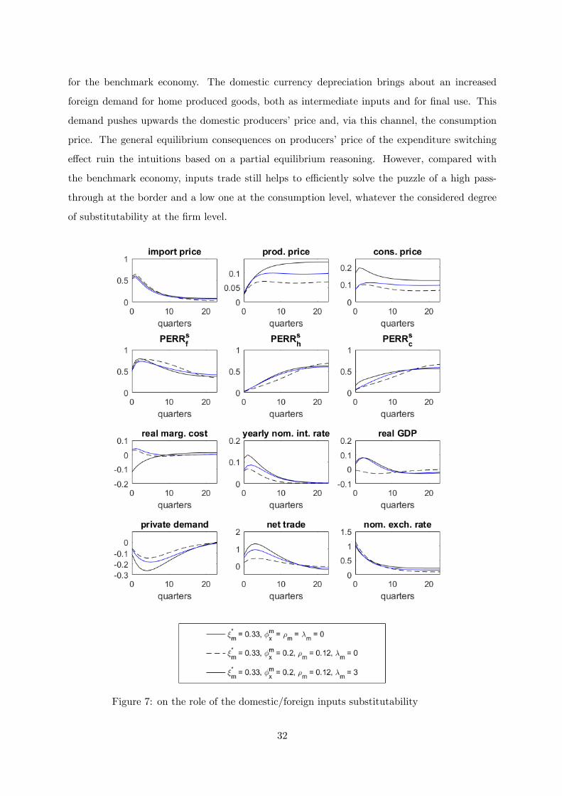
for the benchmark economy. The domestic currency depreciation brings about an increased
foreign demand for home produced goods, both as intermediate inputs and for �nal use. This
demand pushes upwards the domestic producers�price and, via this channel, the consumption
price. The general equilibrium consequences on producers�price of the expenditure switching
e¤ect ruin the intuitions based on a partial equilibrium reasoning. However, compared with
the benchmark economy, inputs trade still helps to e¢ ciently solve the puzzle of a high pass-
through at the border and a low one at the consumption level, whatever the considered degree
of substitutability at the �rm level.
Figure 7: on the role of the domestic/foreign inputs substitutability
32
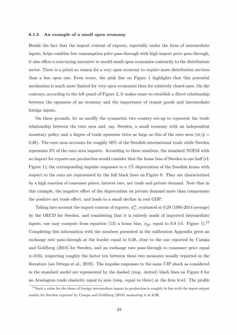
6.1.5 An example of a small open economy
Beside the fact that the import content of exports, especially under the form of intermediate
inputs, helps combine low consumption price pass-through with high import price pass-through,
it also o¤ers a convincing narrative to model small open economies contrarily to the distribution
sector. There is a priori no reason for a very open economy to require more distribution services
than a less open one. Even worse, the pink line on Figure 1 highlights that this potential
mechanism is much more limited for very open economies than for relatively closed ones. On the
contrary, according to the left panel of Figure 2, it makes sense to establish a direct relationship
between the openness of an economy and the importance of transit goods and intermediate
foreign inputs.
On these grounds, let us modify the symmetric two country set-up to represent the trade
relationship between the euro area and, say, Sweden, a small economy with an independent
monetary policy and a degree of trade openness twice as large as this of the euro area ( �m=�y =
0:38). The euro area accounts for roughly 50% of the Swedish international trade while Sweden
represents 3% of the euro area imports. According to these numbers, the standard NOEM with
no import for exports nor production would consider that the home bias of Sweden is one half (cf.
Figure 1); the corresponding impulse responses to a 1% depreciation of the Swedish krona with
respect to the euro are represented by the full black lines on Figure 8. They are characterized
by a high reaction of consumer prices, interest rate, net trade and private demand. Note that in
this example, the negative e¤ect of the depreciation on private demand more than compensate
the positive net trade e¤ect, and leads to a small decline in real GDP.
Taking into account the import content of exports, �mx , evaluated at 0:29 (1995-2014 average)
by the OECD for Sweden, and considering that it is entirely made of imported intermediate
inputs, one may compute from equation (13) a home bias, �H , equal to 0:9 (cf. Figure 1).19
Completing this information with the numbers presented in the calibration Appendix gives an
exchange rate pass-through at the border equal to 0:38, close to the one reported by Campa
and Goldberg (2010) for Sweden, and an exchange rate pass-through to consumer price equal
to 0:04, respecting roughly the factor ten between these two measures usually reported in the
literature (see Ortega et al., 2019). The impulse responses to the same UIP shock as considered
in the standard model are represented by the dashed (resp. dotted) black lines on Figure 8 for
an Armington trade elasticity equal to zero (resp. equal to three) at the �rm level. The pro�le
19Such a value for the share of foreign intermediate inputs in production is roughly in line with the input-output
results for Sweden reported by Campa and Goldberg (2010) measuring it at 0:26.
33
of the price responses is quite di¤erent from the benchmark, with producers�price rising quicker
on impact due to their imported inputs, and stabilizing after one year due to the reaction
of the domestic real activity. As noted earlier, the degree of substitutability between foreign
and domestic inputs matters a lot in this respect: the lower it is, the lower the expenditure
switching e¤ect and the less the depreciation is growth enhancing. The pro�le of the producers�
price is directly transmitted to the consumer price index, of which it constitutes 87%, reducing
considerably the transmission of the exchange rate shock in the short run with respect to the
traditional calibration (full black lines). In the medium to long run, the relationship between
exchange rate and consumption price depends critically on the � and �m trade elasticities. The
goal of the present contribution is only to draw the attention to this point, the next step, left
for future research, would be to try to extract this information from the data by estimating the
full model.
Figure 8: An illustration for a SOE, calibrated on Sweden, interacting with the euro area
In the blue solid lines of Figure 8, we consider a case where the home bias is imposed to be 0:9
by the modeler, without any rigorous calibration of inputs trade. Note that this is equivalent to
considering that the import content of exports, �mx , is equal to 0:74 instead of 0:29 and consists
34
only in transit goods. Such a modelling strategy allows to recover the empirical coherence of
a structural pass-through to import price ten times larger than this to consumption price, but
the corresponding dynamic reactions to an exchange rate shock are exaggeratedly muted by
such an arti�cial isolation of the nominal side of the economy. This illustrates that input trade
helps small open economies to reconcile their large trade openness with a limited transmission
of foreign prices to the consumption price in the short run, delaying it to further horizons via
the larger nominal stickiness observed at the aggregate domestic producing sector level.
6.2 On spillovers
The previous subsection established some important results. First, the conclusions of Corollaries
C1 to C4 still hold in general equilibrium for a set of fairly standard parameters. Second, under
this calibration the intuition behind Proposition 5 is con�rmed, reasserting the important link
between the exchange rate pass-through and the real economy via the expenditure switching
e¤ect. Backing on the pioneering logic of Obstfeld and Rogo¤ (1995), this settles a direct channel
between pass-through and international co-movements, formalized in the following corollary.
Corollary to Proposition 5 In a two-country symmetric framework, any mechanism that
reduces the expenditure switching e¤ect mitigates the terms of trade externality. This enhances
(resp. limits) the international synchronization of real business cycles in the aftermath of country
speci�c shocks to which the country policy rate reacts countercyclically (resp. procyclically). The
last sentence of Proposition 5 states that import contents of exports under the form of either
transit goods or foreign intermediate inputs reduce structurally the aggregate demand externality,
while the distribution sector does not. As a result, one may expect the last mechanism to be more
e¢ cient than the former in eliciting real synchronization, whatever the considered shock.
Let us consider the pure exchange rate shock studied so far that a¤ects both economies in
an inverse way and pushes them on divergent paths. In�ation increases in the economy with a
depreciated currency, depressing its domestic absorption. The larger the expenditure switching
e¤ect, the more this economy adjusts imports downwards and exports upwards, increasing the
chance that depreciation is growth enhancing. As the reverse holds for the trade partner, country
speci�c in�ations and outputs diverge. For this particular shock, any mechanism able to reduce
the expenditure switching e¤ect attenuates the discrepancy as illustrated on Figures 6 and 7.
35

Following Obstfeld and Rogo¤ (1995), the reasoning may be expanded to assess ex-ante the
international consequences of any country-speci�c shock, using the UIP condition. A shock that
pushes the home demand upwards requires more home and foreign productions. This is the
usual aggregate demand externality (cf. e.g. Huang and Liu, 2007) synthesized by parameter
3 in equation (25). If at the same time the monetary authority lowers its policy rate, either
as an endogenous expected reaction or as the initial unexpected shock, the monetary easing
sustains the initial increase in the home economic activity through the implied devaluation,
which handicaps the foreign economy. This is the so-called terms of trade externality. Again, the
larger the expenditure switching e¤ect, the more the terms of trade externality foils the aggregate
demand externality, reducing the capacity of the model to generate ample co-movements. On
the contrary, for all the shocks to which the central bank reacts by pushing the policy rate in
the same direction as this of output, the monetary policy tempers somehow the demand in the
home economy. The larger the expenditure switching e¤ect, the more the implied home currency
devaluation bene�ts to the foreign economic activity.
According to this typology, one expects that all the mechanisms mentioned in Proposition 5
contribute to improve the capacity of a model to generate endogenous co-movements by reducing
the terms of trade externality after country-speci�c monetary policy shocks, productivity shocks
and mark-up shocks.20 On the contrary, they would hinder this possibility in the aftermath of
demand shocks in general. However, note that for shocks emanating directly from the demand
for consumption and investment, the aggregate demand externality plays an important role. A
mechanism that downsizes the elasticity between import and domestic private demand would
inevitably reduce further the potential for demand shocks to drive real business cycles coordi-
nation. All this may be quickly veri�ed with the symmetric two-country model used so far in
Section 6 and running simulations for di¤erent types of shocks. The results of these experi-
ments are displayed in Tables 1 and 2 below, the �rst one focusing on monetary and technology
shocks, and the second one on risk-premium shocks à la Smets and Wouters (2007) and prefer-
ence shocks. The persistence of the exogenous shock processes are �xed at conventional values in
the literature. The two tables report cross-country correlations for real GDP and consumption
prices, and the shock-dependent correlations between exchange rate with import price in�ation
on the one hand and with consumption price in�ation on the other hand. In a two-country
20Following this reasonning, the results obtained in Proposition 5 regarding the role of the demand elasticity of
the CES domestic production function are fully coherent with the conclusion of Burnstein et al. (2008), i.e., that
low substitutability increases the potential of input trade to elicit real business cycle synchronization.
36
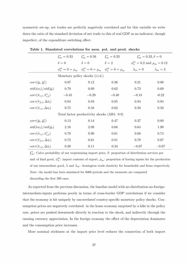
symmetric set-up, net trades are perfectly negatively correlated and for this variable we write
down the ratio of the standard deviation of net trade to this of real GDP as an indicator, though
imperfect, of the expenditure switching e¤ect.
Table 1. Simulated correlations for mon. pol. and prod. shocks
��m = 0:33 ��m = 0:56 ��m = 0:33 ��m = 0:33; � = 0
� = 0 � = 0 � = 2 �mx = 0:2 and �m = 0:12
�mx = 0 = �m �mx = 0 = �m �mx = 0 = �m �m = 0 �m = 3
Monetary policy shocks (i.i.d.)
corr(yt; y�t ) 0:07 0:12 0:36 0:21 0:00
std(nxt)=std(yt) 0:79 0:69 0:62 0:73 0:69
corr(�c;t; ��c;t) �0:45 �0:29 �0:40 �0:18 -0:22
corr(�f;t;�st) 0:94 0:83 0:85 0:94 0:94
corr(�c;t;�st) 0:75 0:58 0:62 0:50 0:50
Total factor productivity shocks (AR1: 0:9)
corr(yt; y�t ) 0:13 0:14 0:47 0:37 0:00
std(nxt)=std(yt) 2:16 2:09 0:68 0:64 1:90
corr(�c;t; ��c;t) 0:78 0:90 0:61 0:68 0:74
corr(�f;t;�st) 0:72 0:61 0:81 0:78 0:67
corr(�c;t;�st) 0:30 0:11 0:34 �0:07 �0:07
��m: Calvo probability of not reoptimizing import price, �: proportion of distribution services per
unit of �nal good, �mx : import contents of export, �m: proportion of foreing inputs for the production
of one intermediate good, � and �m: Armington trade elasticity for households and �rms respectively
Note: the model has been simulated for 6000 periods and the moments are computed
discarding the �rst 500 ones.
As expected from the previous discussion, the baseline model with no-distribution-no-foreign-
intermediate-inputs performs poorly in terms of cross-border GDP correlations if we consider
that the economy is hit uniquely by uncorrelated country-speci�c monetary policy shocks. Con-
sumption prices are negatively correlated: in the home economy surprised by a hike in the policy
rate, prices are pushed downwards directly in reaction to the shock, and indirectly through the
ensuing currency appreciation. In the foreign economy the e¤ect of the depreciation dominates
and the consumption price increases.
More nominal stickiness at the import price level reduces the connection of both import
37

and consumption prices with the exchange rate. The latter point implies an improvement in
the cross-border correlation of consumption price in�ations. The reduction of the expenditure
switching e¤ect observed from the relative volatility of net exports with respect to GDP helps
marginally to increase the GDPs�co-movement. The introduction of a (large) distribution sector
does also reduce the conditional correlation between consumer price in�ation and exchange rate
variations. As for the UIP shock (cf. PERRsf on Figure 6, full blue line), this outcome is obtained
at the cost of a reduction of the link between import price and currency price. This mechanism
does not help much to obtain more cross-border CPI co-movements, but it improves strongly
the GDPs synchronization by reducing the expenditure switching e¤ect. Finally, as long as
perfect complementarity is assumed at the �rm level, import content of exports and production
are also e¢ cient mechanisms to induce endogenous GDPs co-movements. This con�rms the
results obtained by Huang and Liu (2007). However, in their multi-stage production sector with
�rms setting prices according to �xed duration Taylor contract, these authors develop a set-up in
which the importance of intermediate foreign inputs raises together with overall producers�price
stickiness. We show that their results for GDPs synchronization still hold at constant slope for
the aggregate Phillips curve of the production sector. Furthermore, we extend their observations
to the pass-through puzzle. Indeed, foreign value added in domestic production reduces the
consumer price-exchange rate connection while leaving the import price strongly correlated
with the relative price of currency. This helps to improve the cross-border correlation of the
consumption price indices. The last column of the upper part of Table 1 is pretty interesting:
it indicates that when the expenditure switching e¤ect is revitalized via the substitutability
between home and foreign intermediate inputs, the cross border GDP synchronization collapses,
while all the properties observed in the previous column regarding the nominal side of the
economy remain valid. Finally, as highlighted in the Corollary to Proposition 5, the reduction of
the link between import and private aggregate demand induced by the alternatives demand for
import (cf. parameter 3 of equation (25)) limits the aggregate demand externality with respect
to the distribution sector mechanism, explaining the relative poorer performance in terms of real
GDPs coordination.
A home technology shock depresses the producers price and the central bank reacts by
decreasing its policy rate, depreciating the currency. The implied movements in import prices
mitigates somehow the drop in home consumption price while it decreases foreign consumption
prices, yielding a positive wealth e¤ect. For the benchmark NOEM calibration (left column)
such a shock yields some real GDP international co-movement and much more correlation in
38
CPI in�ations. When the import price stickiness is increased from 0:33 to 0:56 the expenditure
switching e¤ect is only slightly a¤ected and real synchronization is not much modi�ed. On the
nominal side, the increased persistence in import price emphasizes the above described import
price e¤ect and the CPI in�ations are even more connected. The distribution sector operates
exactly in the other direction: it strongly decreases the expenditure switching e¤ect, tuning down
the terms of trade externality and improving real co-movements. On the nominal side, as the
home economy exports less, domestic producers�prices decrease further, the central bank lowers
even more its policy rate. Among the drivers of the import price, the increase in the marginal
cost of the foreign producers more than compensates the reduction in the price of domestic
distribution services and the import price-exchange rate correlation increases relatively to the
benchmark NOEM. However, due to the relative drop in producers�prices, this is not translated
in the same proportion into an increased CPI-exchange rate correlation. In the foreign economy
the wealth e¤ect of the appreciation increases, but this demand is now more ful�lled by foreign
producers whose prices increase. In the end, the cross-border CPI in�ations correlation turns out
to be somewhat lower. Input trade produces very similar outcomes on the real side: under perfect
complementarity of home/foreign intermediate inputs the terms of trade externality is strongly
reduced and real outputs synchronization is enhanced.21 As already displayed and discussed by
Burstein, Kurtz and Tesar (2008) for technology shocks, and for the reasons made explicit in
Proposition 5, the more �rms have the possibility to switch between foreign and domestic inputs,
the lower the cross-border real correlation. On the nominal side, the input trade story is pretty
di¤erent from the distribution services one. The home currency depreciation rises the price of
the foreign intermediate input, braking the drop of domestic producers�marginal cost. At the
same time, the share of import price in the CPI index drops from 0:26 to 0:10, closing down the
CPI-exchange rate correlation independently of the degree of substitutability �m. Corollary to
Proposition 5 is still veri�ed for technology shocks that typically move economic activity and
the policy interest rate in opposite directions and input trade is the only mechanism allowing
to combine low exchange rate-CPI correlation while keeping a high exchange rate-import price
interrelationship.
Table 2 displays the same co-movements statistics for a Smets and Wouters (2007) risk-
premium shock, i.e. a shock that drives a wedge between the central bank risk-free rate and
the interest rate actually faced by households. Such a shock has the distinctive feature of
21Even though somewhat less than under the distribution sector mechanism, due to the above mentionned
decrease in aggregate demand externality, via parameter 3 (equation (25)).
39

moving investment and consumption together. The Corollary to Proposition 5 also applies to
this shock to which the policy rate reacts procyclically. If the risk-premium narrows in the home
economy, home domestic demand increases together with the demand for imports which is pushed
even further by the home currency appreciation resulting from the central bank endogenous
reaction. Confronted with increased import prices and home economy external demand, the
foreign economy reduces its own domestic demand. The strong positive GDPs correlation is
entirely driven by the respective net trades that slow down the home GDP and encourage the
foreign one. Any mechanism that reduces the terms of trade externality tends to decrease this
positive correlation and it is more particularly the case for the foreign intermediate inputs than
for the distribution sector, as the former also reduces the import elasticity to absorption, 3(cf.
Proposition 5), and therefore the aggregate demand externality. Under input trade (last two
columns on the right), the decrease in import price implied by the initial shock a¤ects the
producers�marginal cost and calm down their price increase compared to the other models.
This is translated in the CPI index with a larger weight as the home bias increases from 0:74
to 0:90, reducing the conditional correlation between consumption price and exchange rate and
eliciting cross-border CPIs�correlation.
40
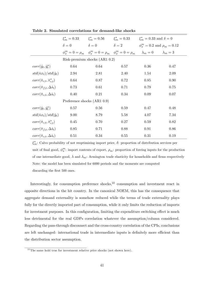
Table 2. Simulated correlations for demand-like shocks
��m = 0:33 ��m = 0:56 ��m = 0:33 ��m = 0:33 and � = 0
� = 0 � = 0 � = 2 �mx = 0:2 and �m = 0:12
�mx = 0 = �m �mx = 0 = �m �mx = 0 = �m �m = 0 �m = 3
Risk-premium shocks (AR1 0.2)
corr(yt; y�t ) 0:64 0:64 0:57 0:36 0:47
std(nxt)=std(yt) 2:94 2:81 2:40 1:54 2:09
corr(�c;t; ��c;t) 0:64 0:87 0:72 0:85 0:90
corr(�f;t;�st) 0:73 0:61 0:71 0:79 0:75
corr(�c;t;�st) 0:40 0:21 0:34 0:09 0:07
Preference shocks (AR1 0.9)
corr(yt; y�t ) 0:57 0:56 0:59 0:47 0:48
std(nxt)=std(yt) 9:00 8:79 5:58 4:07 7:34
corr(�c;t; ��c;t) 0:45 0:70 0:27 0:59 0:82
corr(�f;t;�st) 0:85 0:71 0:88 0:91 0:86
corr(�c;t;�st) 0:51 0:34 0:55 0:31 0:19
��m: Calvo probability of not reoptimizing import price, �: proportion of distribution services per
unit of �nal good, �mx : import contents of export, �m: proportion of foreing inputs for the production
of one intermediate good, � and �m: Armington trade elasticity for households and �rms respectively
Note: the model has been simulated for 6000 periods and the moments are computed
discarding the �rst 500 ones.
Interestingly, for consumption preference shocks,22 consumption and investment react in
opposite directions in the hit country. In the canonical NOEM, this has the consequence that
aggregate demand externality is somehow reduced while the terms of trade externality plays
fully for the directly imported part of consumption, while it only limits the reduction of imports
for investment purposes. In this con�guration, limiting the expenditure switching e¤ect is much
less detrimental for the real GDPs correlation whatever the assumption/column considered.
Regarding the pass-through disconnect and the cross-country correlation of the CPIs, conclusions
are left unchanged: international trade in intermediate inputs is de�nitely more e¢ cient than
the distribution sector assumption.
22The same hold true for investment relative price shocks (not shown here).
41
7 Conclusion
In the previous lines we have tried to better understand the respective macroeconomic impli-
cations of a distribution sector and of the inclusion of foreign inputs in production before price
di¤erentiation. The �rst mechanism has usually been advocated to be e¢ cient in solving the
exchange rate pass-through puzzle and the second one to signi�cantly improve the international
synchronization of business cycles. Our systematic comparison brings the surprising conclusion
that the allocation of roles should actually be reversed. The distribution sector is very good
at mitigating the connection between the exchange rate and the consumption price, but this
occurs via an attenuation of the exchange rate/import price relationship, in opposition to em-
pirical evidence. On the contrary, this mechanism is pretty e¢ cient in generating cross-border
real spillovers after country speci�c shocks. It improves strongly spillovers after shocks that
move output and the relative price of currency in opposite directions and they are not much
deteriorated, if at all, after demand-like shocks.
This reversal of the outcome with respect to the primary goal also holds for input trade,
that is the inclusion of import price in the marginal cost of domestic producers with a market
power and staggered prices. It systematically reduces the link between consumption price and
exchange rate in the short run without a¤ecting the strong relationship between import price
and exchange rate. For all the shocks considered, the mechanism increases the cross-border
correlation between consumption prices. Under perfect complementarity, it is also e¢ cient in
improving the synchronization of the real economic activity except after demand-like shocks. In
our view, the input trade mechanism provides a strong economic rationale for potentially high
home bias even for the very open economies, with all the bene�ts in terms of exchange rate
disconnect it may imply.
The ultimate test would be to bring the model to the data and to check how a two-country
estimated model endowed with the two channels discussed at length in this paper allows to
indeed (i) improve the estimation of both the import and consumption price dynamics and (ii)
increase the real and nominal synchronization of macro-variables. This is at the agenda of future
research.
42

References
[1] Adolfson, M., Laseen, S. Linde, J. and Villani, M. (2008), �Evaluating an estimated New
Keynesian small open economy model�, Journal of Economic Dynamics and Control 32, 8,
2690-2721.
[2] Amador, J., Cappariello, R. and Stherer, R. (2015), �Global value chains: a view from the
euro area�, Asian Economic Journal, 29, 2, 99-120.
[3] Berman, N., Martin, P. and Mayer, T. (2012). �How do di¤erent exporters react to exchange
rate changes?�, Quarterly Journal of Economics, 127, 1, 437�492.
[4] Bils, M. and Klenow, P. (2004), �Some evidence on the importance of sticky prices�, Journal
of Political Economy, 112, 5, 937-985.
[5] Burstein, A., Neves, J. and Rebelo, S. (2003), �Distribution costs and real exchange rate
dynamics during exchange-rate-based stabilizations�, Journal of Monetary Economics, 50,
6, 1189-1214.
[6] Burstein, A., Kurz, C. and Tesar, L. (2008), �Trade, production sharing, and the interna-
tional transmission of business cycles�, Journal of Monetary Economics, 55, 4, 775-795.
[7] Burstein, A. and Gopinath, G. (2014), �International prices and exchange rates�, Handbook
of International Economics, Elsevier.
[8] Calvo, G.A. (1983), �Staggered prices in a utility-maximizing framework�, Journal of Mon-
etary Economics, 12, 3, 383-398.
[9] Campa, J. and Goldberg, L. (2005), �Exchange rate pass-through into import prices�,
Review of Economics and Statistics, 87, 4, 679�690.
[10] Campa, J. and Goldberg, L. (2010), �The sensitivity of the CPI to exchage rates: distrib-
ution margins, imported inputs and trade exposure�, Review of Economics and Statistics,
92, 2, 392�407.
[11] Christiano, L., Eichenbaum, M. and Evans, C. (2005), �Nominal rigidities and the dynamic
e¤ects of a shock to monetary policy�, Journal of Political Economy, 113, 1, 1-45.
[12] Corsetti, G. and Dedola, L. (2005), �A macroeconomic model of international price dis-
crimination�, Journal of International Economics, 67, 1, 129-155.
43
[13] Corsetti, G., Dedola, L. and Leduc, S. (2008), �High exchange-rate volatility and low pass-
through�, Journal of Monetary Economics, 55, 6, 1113-1128.
[14] Dedola, L. and Lombardo, G. (2013), �Financial frictions, �nancial integration and the
international propagation of shocks�, Economic Policy, 27, 70, 319-359.
[15] de Walque, G., Jean�ls, Ph., Lejeune, T., Rychalovska, Y. and Wouters, R. (2017), An
estimated two-country EA-US model with limited exchange rate pass-through, NBB WP
n�317.
[16] Dotsey, M. and King, R. (2005), �Implications of state-dependent pricing for dynamic
macroeconomic models�, Journal of Monetary Economics, 52, 1, 213-242.
[17] Eichenbaum, M. and Fisher, J. (2007), �Estimating the frequency of price re-optimization
in Calvo-style models�, Journal of Monetary Economics, 54, 7, 2032-2047.
[18] Erceg, C., Guerrierri, L. and Gust, C. (2006), �SIGMA: a new open economy model for
policy analysis�, International Journal of Central Banking, 2, 1, 1-50.
[19] Eyquem, A. and Kamber, G. (2014), �A note on the business cycle implications of trade in
intermediate goods�, Macroeconomic Dynamics, 18, 1172-1186.
[20] Fagan, G., Henry, J. and Mestre, R. (2005), �An area-wide model for the auro area�,
Economic Modelling, 22, 39-59.
[21] Feenstra, R.C. (1998), �Integration of trade and disintegration of production in the global
economy�, Journal of Economic Perspectives, 12, 31-50.
[22] Georgiadis, G., Gräb, J. and Khalil, M. (2018), Global value chain participation and ex-
change rate pass-through, ECB mimeo.
[23] Gust, C., Leduc, S. and Vigfusson, R. (2010), �Trade integration, competition, and the
decline in exchange-rate pass-through�, Journal of Monetary Economics 57, 3, 309-324.
[24] Huang, K. and Liu, Z. (2001), �Productions chain and general equilibrium aggregate dy-
namics�, Journal of Monetary Economics, 48, 437-462.
[25] Huang, K. and Liu, Z. (2007), �Business cycles with staggered prices and international
trade in intermediate inputs�, Journal of Monetary Economics, 54, 1271-1289.
44

[26] Jean�ls, Ph. (2008), Imperfect exchange rate pass-through : the role of distribution services
and variable demand elasticity, NBB WP n�135.
[27] Johnson, R. (2014), �Trade in intermediate inputs and business cycle comovement�, Amer-
ican Economic Journal: Macroeconomics, American Economic Association, 6, 4, 39-83.
[28] Kamber, G. and Thoenissen, C. (2013), �Financial exposure and the international trans-
mission of �nancial shocks�, Journal of Money, Credit and Banking 45, s2, 159-195.
[29] Kimball, M. (1995), �The quantitative analytics of the basic neomonetarist model�, Journal
of Money, Credit and Banking, 27, 4, 1241�1277.
[30] Kollman, R. (2013), �Global banks, �nancial shocks and international business cycles: evi-
dence from an estimated model�, Journal of Money, Credit and Banking, 45, s2, 159-195.
[31] Lane, Ph. and Stracca, L. (2018), �Can appreciation be expansionary? Evidence from the
euro area�, Economic Policy, 33, 1, 225-264.
[32] Obstfeld, M. and Rogo¤, K. (1995), �Exchange rate dynamics redux�, Journal of Political
Economy, 103, 3, 624-660.
[33] Ortega, E., Osbat, C. Rubene, I., Gunnella, V., Pisani, M., Comunale, M., Bruha, J. and
Mavromatis, K. (2019), Exchange rate pass-through in the euro area and EU countries,
ECB Occasional Paper (forthcoming).
[34] Özyurt, S. (2016), Has the exchange rate pass-through recently declined in the euro area?,
ECB WP n�1955:
[35] Schmitt-Grohe, S. and Uribe, M. (2001), �Stabilization policy and the costs of dollariza-
tion�, Journal of Money, Credit and Banking 33, 2, 482-509.
[36] Shambaugh, J. (2008), �A new look at pass-through�, Journal of International Money and
Finance, 27, 560-591.
[37] Shi, K. and Xu, J. (2010), �Intermediate goods trade and exchange rate pass-through�,
Journal of Macroeconomics, 32, 571-583.
[38] Smets, F. and Wouters, R. (2002), �Openness, imperfect exchange rate pass-through and
monetary policy�, Journal of Monetary Economics 49, 5, 947-981.
45
[39] Smets, F. and Wouters, R. (2007), �Shocks and frictions in US business cycles: A Bayesian
DSGE approach�, American Economic Review 97, 3, 586-606.
[40] Taylor, J. (1980), �Aggregate Dynamics and Staggered Contracts�, Journal of Political
Economy, 88, 1, 1-24.
[41] van der Helm, R. and Hoekstra, R. (2009), �Attributing GDP growth of the euro area to �nal
demand categories�, Paper prepared for the 17th international input-output conference,
July 13-17th, Sao Paulo, Brazil, Statistics Netherlands.
[42] Wang, J. (2010), �Home bias, exchange rate disconnect, and optimal exchange rate policy�,
Journal of International Money and Finance, 29, 55-78.
[43] Yi, K.-M. (2003), �Can vertical specialization explain the growth of world trade?, Journal
of Political Economy, 111, 1, 52-102.
46
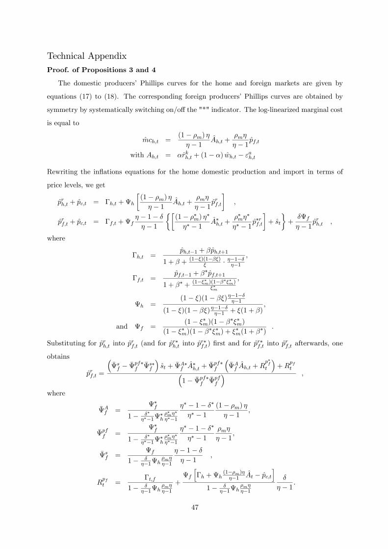
Technical AppendixProof. of Propositions 3 and 4
The domestic producers� Phillips curves for the home and foreign markets are given by
equations (17) to (18). The corresponding foreign producers�Phillips curves are obtained by
symmetry by systematically switching on/o¤ the "*" indicator. The log-linearized marginal cost
is equal to
mch;t =(1� �m) �� � 1 Ah;t +
�m�
� � 1 pf;t
with Ah;t = �rkh;t + (1� �) wh;t � "ah;t
Rewriting the in�ations equations for the home domestic production and import in terms of
price levels, we get
prh;t + pc;t = �h;t +h
�(1� �m) �� � 1 Ah;t +
�m�
� � 1 prf;t
�,
prf;t + pc;t = �f;t +f� � 1� �� � 1
��(1� ��m) ���� � 1 A�h;t +
��m��
�� � 1 p�rf;t
�+ st
�+�f� � 1 p
rh;t ,
where
�h;t =ph;t�1 + �ph;t+1
1 + � + (1��)(1���)� � ��1����1
;
�f;t =pf;t�1 + �
�pf;t+1
1 + �� + (1���m)(1�����m)��m
;
h =(1� �)(1� ��)��1����1
(1� �)(1� ��)��1����1 + �(1 + �);
and f =(1� ��m)(1� ����m)
(1� ��m)(1� ����m) + ��m(1 + ��).
Substituting for prh;t into prf;t (and for p
r�h;t into p
r�f;t) �rst and for p
r�f;t into p
rf;t afterwards, one
obtains
prf;t =
��sf � �pf�f
�s�f
�st + �A�f A
�h;t +
�pf�f
��Af Ah;t +R
p�ft
�+R
pft�
1� �pf�f�pff
� ,
where
�Af =�f
1� ��
���1�h��m�
�
���1
�� � 1� ��
�� � 1(1� �m) �� � 1 ,
�pff =�f
1� ��
���1�h��m�
�
���1
�� � 1� ��
�� � 1�m�
� � 1 ,
�sf =f
1� ���1h
�m���1
� � 1� �� � 1 ,
Rpft =
�t;f
1� ���1h
�m���1
+f
h�h +h
(1��m)���1 At � pc;t
i1� �
��1h�m���1
�
� � 1 .
47
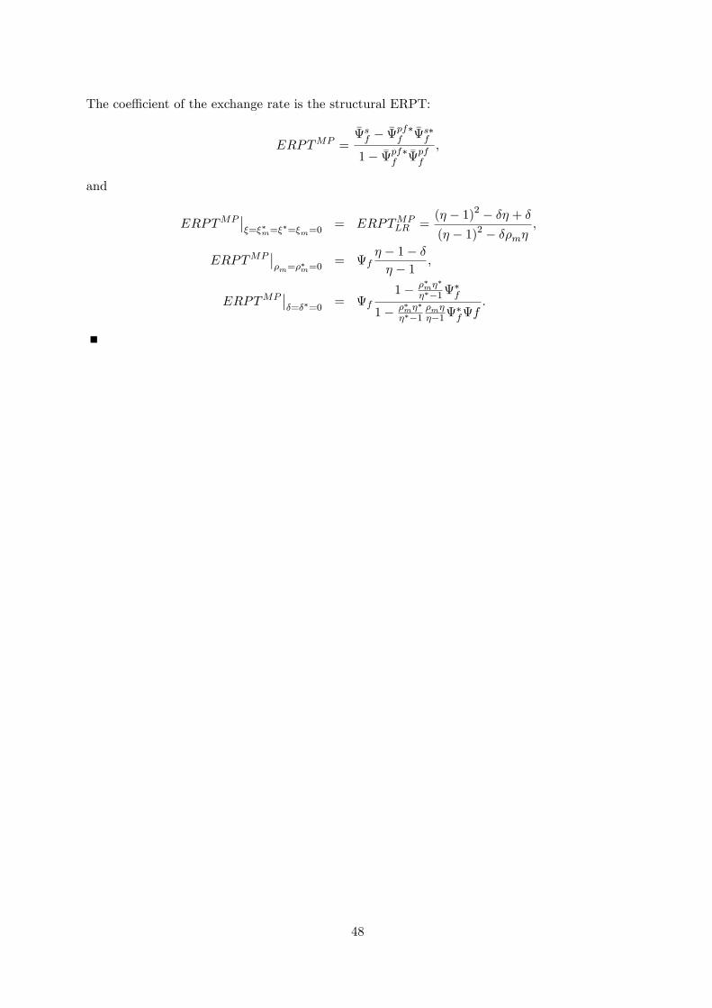
The coe¢ cient of the exchange rate is the structural ERPT:
ERPTMP =�sf � �pf�f
�s�f
1� �pf�f�pff
,
and
ERPTMP���=��m=�
�=�m=0= ERPTMP
LR =(� � 1)2 � �� + �(� � 1)2 � ��m�
,
ERPTMP���m=�
�m=0
= f� � 1� �� � 1 ,
ERPTMP���=��=0
= f1� ��m�
�
���1�f
1� ��m��
���1�m���1
�ff
.
48

Calibration of the two-country model
Table A1: Calibration of the two-country symmetric model (on euro area)
Big ratios Monetary policy
�c�y 0:56 interest rate persistence (�r) 0:9
�{�y 0:20 reaction to in�ation (��) 1:6
�m�y 0:20 reaction to output gap (�yg) 0:1
reaction to output gap variation (��yg) 0:1
Households Firms
external habit 0:7 Cobb-Douglas capital share (�) 0:33
hh relative risk aversion 1:2 capital depreciation rate 0:025
inv. elast. of e¤ort w.r.t. wage 2 inv. adjustment cost 4
Calvo prob. wage 0:75 demand price elasticity (�) 4:5
hh Armington trade elasticity (�) 3 Calvo prob. dom. price (�) 0:75
foreign/dom. goods adjust. cost 4 Calvo prob. imp. price (��m) 0:33
�rms�Armington trade elasticity (�m) 3 or 0
foreign/dom. goods adjust. cost 4
49