Low Reynolds Number Numerical Simulation of the

International Journal of Aviation, International Journal of Aviation,

Aeronautics, and Aerospace Aeronautics, and Aerospace

Volume 5 Issue 1 Article 8

2-21-2018

Low Reynolds Number Numerical Simulation of the Aerodynamic Low Reynolds Number Numerical Simulation of the Aerodynamic

Coefficients of a 3D Wing Coefficients of a 3D Wing

Khurshid Malik International Islamic University - Malaysia, [email protected] Waqar Asrar International Islamic University - Malaysia, [email protected] Erwin Sulaeman International Islamic University Malaysia, [email protected]

Follow this and additional works at: https://commons.erau.edu/ijaaa

Part of the Aerodynamics and Fluid Mechanics Commons

Scholarly Commons Citation Scholarly Commons Citation Malik, K., Asrar, W., & Sulaeman, E. (2018). Low Reynolds Number Numerical Simulation of the Aerodynamic Coefficients of a 3D Wing. International Journal of Aviation, Aeronautics, and Aerospace, 5(1). https://doi.org/10.15394/ijaaa.2018.1209

This Article is brought to you for free and open access by the Journals at Scholarly Commons. It has been accepted for inclusion in International Journal of Aviation, Aeronautics, and Aerospace by an authorized administrator of Scholarly Commons. For more information, please contact [email protected].

http://commons.erau.edu/

http://commons.erau.edu/

https://commons.erau.edu/ijaaa

https://commons.erau.edu/ijaaa

https://commons.erau.edu/ijaaa/vol5

https://commons.erau.edu/ijaaa/vol5/iss1

https://commons.erau.edu/ijaaa/vol5/iss1/8

https://commons.erau.edu/ijaaa?utm_source=commons.erau.edu%2Fijaaa%2Fvol5%2Fiss1%2F8&utm_medium=PDF&utm_campaign=PDFCoverPages

http://network.bepress.com/hgg/discipline/222?utm_source=commons.erau.edu%2Fijaaa%2Fvol5%2Fiss1%2F8&utm_medium=PDF&utm_campaign=PDFCoverPages

https://doi.org/10.15394/ijaaa.2018.1209

mailto:[email protected]

Historically, a large number of studies have been done on the capability of

simulation as a key tool in predicting aerodynamic behavior (Anderson, 2003;

Anderson et al., 1995) to determine the overall performance and stability of an

airplane, Unmanned Aerial Vehicle (UAV) and Micro Air Vehicle MAV. The

simulation consisting of the six aerodynamic components and their derivatives are

vital which may be obtained from wind tunnel experiments as well as through

Computational Fluid Dynamics (CFD) simulation (note: Please see appendix 1 for

terminology).

CFD can be used for the prediction of aerodynamic properties for 2D or 3D

wings. Several studies have been done on 2D/3D finite wings to investigate the

ability of STAR CCM+ to compute lift, drag, and pitching moments. (Sagmo et al.,

2016, Bui, 2016, Garcia et al., 2016, Shankara and Snyder, 2012, Narayana et al.,

2005).

Experimental data on the three main aerodynamic components; lift

coefficient (CL), drag coefficient (CD) and pitching moment coefficient (CM) on a

flat plate wing at low Reynolds numbers have been made available in the literature

by (Ananda et al., 2015, Pelletier and Mueller, 2000, Shields and Mohseni, 2012).

The behavior of a 3D wing, analyzing the forces (lift, drag & normal) on several

finite wings of small to large aspect ratio has been experimentally investigated at

low Reynolds number (Ortiz et al., 2015). Their results stated that lift to drag ratio

(L/D ratio) follows the inverse tangent of the angle of incidence for almost all

experimental cases.

Wind tunnel experiment on ten flat plates with different taper ratios (λ) 0.5,

0.75, & 1 and aspect ratio (AR) 2, 3, 4, & 5 was carried out at Reynolds number

ranging from 5 × 104 to 1.5 × 105 by Ananda et al., 2015, using a three-

component force balance. Similar work on the rectangular and tapered flat plate

wings (AR=0.75, 1, 1.5, and 3) were performed at Reynolds numbers between

5 × 104 and 1 × 105 in a wind tunnel by (Shields and Mohseni, 2012). The result

of CL, CD and CM variation with angle of attack and Reynolds number was

presented.

Mueller and Delauier, (2003), Pelletier and Mueller, (2000), experimentally

measured CL, CD and CM for various thin flat plates and cambered plates at Reynolds

numbers from 6 × 104 to 2 × 105. A detailed aerodynamic study has been

performed by (Abe, 2003) on different aspect ratio flat plates and cambered airfoils

at Reynolds numbers below 105 using two mechanical balance devices. Only

CL, CD, CM & roll moment coefficient (Cl) were measured using the two devices.

One device measures the CL & CD, and another device extracts the CM & Cl.

1

Malik et al.: SIMULATION OF A 3D WING

Published by Scholarly Commons, 2018

To estimate the low-speed longitudinal aerodynamic characteristics, a flat-

plate model of an advanced fighter configuration was experimented in the NASA

Langley Subsonic Basic Research Tunnel. Low-speed longitudinal aerodynamic

data were measured over a range of angles of attack from 0° to 40° and freestream

dynamic pressures from 7.5 psf to 30 psf (M = 0.07 to M = 0.14). They are presented

as CL, CD, CM and flow-visualization (McGrath et al., 1994).

CL, CD and CM investigation were studied on square plates mounted in a

Low-Speed Wind Tunnel (Fail el al., 1959). Study on the flat plate wing was done

using a hybrid continuum–particle approach for flows having a Reynolds number

varying between 1 and 200 and a Mach number of 0.2 (Sun and Boyd, 2004).

Laitone (1997) performed low turbulence wind tunnel testing on NACA 0012

rectangular wing at a low Reynolds number of 2 × 104. He measured only

CL, CD and compared with thin flat and cambered plates. The result indicated that

thin plate with 5% circular arc camber showed the best profile for Reynolds number

below 7 × 104 (Laitone, 1997).

This paper presents a CFD study of a finite flat plate wing to estimate the

six aerodynamic coefficients and their derivatives at a Reynolds number of 3 × 105

based on the chord length and free stream conditions. To the best of Authors

‘knowledge, most of the work on flat plate wings in the open literature report the

three components (lift, drag and pitching moment). It seems that there is a lack of

data on six aerodynamic coefficients and stability derivatives for a low aspect ratio

flat plate wing at low Reynolds number. This data is of vital importance in low-

speed aerodynamics and design for applications to MAVs and UAVs.

Method

For efficient CFD analysis, CFD geometry fidelity must be as precise as

possible. Experience, skill and proper assessment of the effect of flow condition

selection are required to study geometry simplification versus fidelity (Rumsey et

al., 2011). There are three major steps: 1) Pre-processing, 2) Numerical

simulation/Processing, and 3) Post-processing/Result. In pre-processing, a 3-D

model was developed using Solid Works. Then boundary and operating condition

on unstructured meshing were performed using STAR-CCM+.

Model Details

A flat plate 3D wing model is selected for this study. It has an aspect ratio

of three with no taper. Table 1 shows the 3D flat plate wing model specification.

The model and computational domain are shown in Figure 1.

2

International Journal of Aviation, Aeronautics, and Aerospace, Vol. 5 [2018], Iss. 1, Art. 8

https://commons.erau.edu/ijaaa/vol5/iss1/8DOI: https://doi.org/10.15394/ijaaa.2018.1209

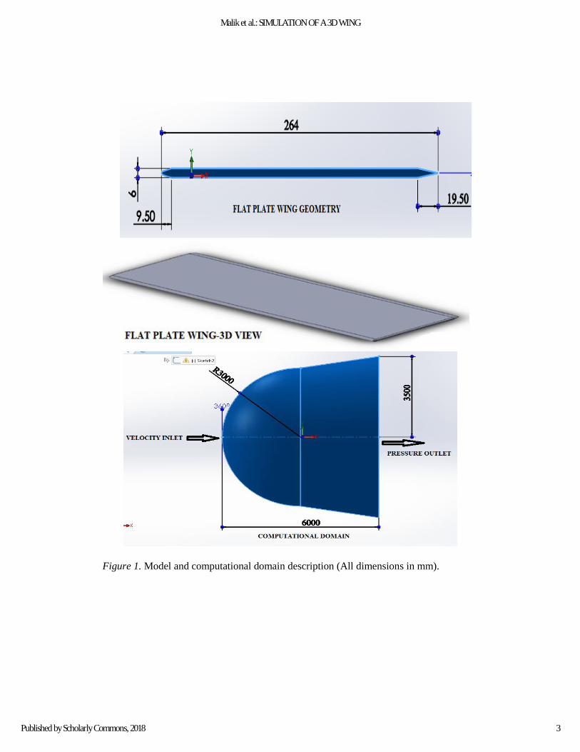
Figure 1. Model and computational domain description (All dimensions in mm).

3



Table 1

3D flat plate wing specification

Model: 3D Flat plate wing

Chord (c) 0.264 m

Area (A) 0.2122 m2

Span (b) 0.804 m

Aspect Ratio 3

Reynolds number 3 × 105

Mesh Details

The three-dimensional viscous, incompressible flow over the flat plate wing

was simulated in STAR CCM+. It is also used to generate the computational mesh

of the flat plate wing as the pre-processor. This consist of several types of volume

and surface mesh which are trimmed, tetrahedral and polyhedral. The polyhedral

method (a volume with 14 faces) was chosen because of its ability to fit around the

leading and trailing edges of the grid. Aerodynamic data can be achieved near wind

tunnel experiment using unstructured polyhedral meshing with steady-state RANS

(Reynolds-Averaged Navier-Stokes) approach and K-Omega SST turbulence

model (Sagmo et al., 2016, Bui, 2016, Garcia et al., 2016, Shankara and Snyder,

2012, Narayana et al., 2005). An unstructured 3D mesh was generated for the flat

plate wing in the computational domain. Approximately 15, 00,000 mesh count was

used in the polyhedral elements. There is an additional benefit of using the

polyhedral meshing because it is computationally more efficient compared to

another type of mesh. Figure 2 illustrates the surface and volume mesh and plane

section and mesh near the LE and TE. The prism layer is selected with 0.032Cref

thickness, and a total number of 12 layers is used to capture the flow near the wall.

In Figure 2, the boundary layer mesh has been shown for a closer view. Table 2

shows the main meshing parameters which are used in the simulation.

4



Table 2

Mesh Parameters

Number of Cells 4.1M

Number of Surface Faces 26.4M

Target Prism Layer Height 0.032Cref

Number of Prism Layers 12

Number of Vertices 21.6M

Figure 2. Flat plate wing meshing

Simulation physics

To set up an incompressible aerodynamics model using the steady-state

RANS approach, the physics model details are presented in Table 3. The Spalart-

Allmaras turbulence flow model was used. The Spalart-Allmaras turbulence model

can be used in cases of streamlined geometries without large base separation

regions. This model works best for attached boundary layers or mildly separated

flows (that is, flow past a wing at or below stall). This model is specially designed

5



for aerospace applications in the wall boundary flows, which is mainly used to

properly solve the areas of the boundary layer that is affected by viscosity and has

good convergence toward solid wall turbulent flow. It has the benefit of being

readily employed in an unstructured CFD solver. It has become a popular model in

unstructured CFD methods in the aerospace industry (Baldwin and Lomax, 1978,

Johnson and King, 1985). Spalart-Allmaras and Realizable k-epsilon Turbulence

models showed good results for 2D and 3D wing models at low Reynolds number

(Sagmo et al., 2016)

Table 3

Physics setup

Group Box Model

Space Three Dimensional

Time Steady

Material Gas-Air

Flow Segregated Flow

Equation of State Constant Density

Viscous Regime Turbulent

Turbulence

Reynolds-Averaged

Navier-Stokes

Spalart-Allmaras

Results and Discussion

Three-dimensional steady turbulent flow at constant density was selected,

and no-slip wall boundary conditions are applied at the wing surface with velocity

inlet and pressure outlet boundary conditions. Flat plate wing simulations were

performed and ran for 1,500 to 2,000-time iteration (steps) for each case of study.

The quarter chord point on the wing was used as the moment reference point and

the point of rotation. One case simulation run time was between 8 to 20 hours.

After 1500-time iterations, the aerodynamic coefficients of flat plate wing

reached a constant value for angles of attack from −10𝑜 to 10𝑜. Beyond an angle

of attack of ± 10°, small variations in yaw moment coefficient (𝐶𝑁), roll moment

coefficient (𝐶𝑙) and side force coefficient (𝐶𝑌) are present even after 2500

iterations.

6



In the next sections, firstly, the validation results are discussed. Six

component results (effect of pitch angle) are discussed when only the pitch angle

(α) is varying. The roll (β) and yaw angles (γ) are zero for this part. Six components

result for cases of yaw, roll and the combination of all three angles (effect of yaw,

roll and pitch angles) will also be presented. Finally, flat plate wing aerodynamic

stability derivatives in the linear portions of the graphs for all aerodynamic

components are presented.

Validation of Simulation Data

For validation of the CFD solution, a case study was done on the rectangular

flat-plate AR-3 wing at a Reynolds number of 80,000. The CL, CD, and CM results

from the CFD simulation are plotted in Figs. 3 (a & b) and 4 with the experimental

data for the same wing at the same Re available in the open literature (Ananda et

al., 2015, Pelletier and Mueller, 2000, Shields and Mohseni, 2012). The CFD

simulation results agree quite well with the experimental values.

The flat plate wing experimental data by Ananda et al., 2015, was obtained

using a UIUCLRN-FB three-component wind tunnel force balance at Re 80,000.

The differences between the AR-3 wing tested with the UIUCLRN-FB (Ananda et

al., 2015) and the wing tested by (Pelletier and Mueller, 2000 and Shields and

Mohseni, 2012), is that, Ananda used a wing with 4.3% thickness-to-chord ratio

and 10-to-1 elliptical trailing edge thickness ratio compared to 2.6% and 5-to-1

ratios in the flat plate wing used by Pelletier and Mueller, 2000 and Shields and

Mohseni, 2012 respectively. Lift, drag, and pitching moment comparison results

are shown in the Figs. 3 (a & b) and 4.

The lift and drag coefficients plotted in Figure 3(a) show close agreement

between the CFD results [see Figure 3(a)] and the experimental data from (Ananda

et al., 2015, Pelletier and Mueller, 2000, Shields and Mohseni, 2012). The slight

differences found near the stall angle of attack and maximum lift coefficient

(𝐶𝐿 𝑚𝑎𝑥) may be because of the differences in the model’s geometry and mesh

design. Similarly, 𝐶𝐷 [Figure3(b)] shows good agreement with the experimental

results. The minimum drag coefficient (𝐶𝐷 𝑚𝑖𝑛) from (CFD data & Ananda et al.,

2015) are also found to be within the expected minimum drag range for a theoretical

flat-plate wing at the same Reynolds numbers. The CFD data and the experimental

data of Shields and Mohseni, 2012, show a slight disagreement. The CM versus α is

shown and validated in Figure 4 with data from (Ananda et al., 2015, Pelletier and

Mueller, 2000, Shields and Mohseni, 2012). These results show slight differences

that can be attributed to the geometry and mesh variations, including the differences

in the three wind tunnels and test models as also suggested by Shields and Mohseni,

2012.

7



The pitching moment (𝐶𝑀 is measured at the quarter chord from the leading

edge of the wing) results suggest that although the moment is approximately close

to zero for low angles of attack as shown in Figure 4, there is a variation in 𝐶𝑀 as a

function of the angle of attack. Figs. 3 (a & b) and 4, illustrate the results of the

simulations of the 𝐶𝐿 , 𝐶𝐷, and 𝐶𝑀 for a Reynolds number 80,000 and all data is

reproduced here to illustrate the effectiveness of STAR CCM+ as a CFD tool as its

results are validated with available experimental data for the flat plate wing of AR

3.

Figure 3. (a) Variation on lift coefficient and (b) drag coefficient with aoa

8



Figure 4. Variation of pitching moment coefficient with aoa

Effect of Pitch Angle

This section of the paper describes the behavior of the six aerodynamic

force and moment components (CL, CD, CM, CN, Cl & CY) of a flat plate 3D wing at

a Reynolds number of 3 × 105 with respect to variations in the angle of pitch. The

important characteristics discussed in this case relates to the maximum lift

coefficient and the lift curve slope. The angle of attack (pitch angle) was varied

from −200to 250. to identify post-stall effects of the flat-plate wing.

Lift, drag, and moment curves of the flat-plate wing are shown in Figs. 5 (a

& b) and 6(a). The CLmax for the flat plate wing was found be in the range of 0.67

to 0.7 at an angle of attack around 150. Before stall, the quarter-chord CM was

observed to be small for flat plate wing. In the post-stall regions, large negative

CM was found with larger magnitude [see Figure6(a)]. In the post-stall region, CL

and CM were found to be slightly constant over the range of angles of attack tested

(up to 25o). As shown in Figure 5(b), The CDmin values are estimated to be

approximately between 0.01 to 0.02.

9



CN, Cl, and CY, have perhaps not been previously reported for a flat plate

wing in the open literature. They are important factors in stability and control (Hull,

2007). As shown in Figure 6(b), The side force coefficient CY was mostly constant

with slight variations in the range of angle of attack from −100to 250, was

consistently close to zero. Some variation is found in CY at angles of attack below

−100.

The rolling moment Cl is plotted in Figure 7(a) for angles of attack from

−100 to 100. The value of the Cl was found approximately to be nearly zero

(±0.00005) with a slight increment for the range of angle of attack −80 to 80. In

contrast, a negative graph (value lying between -0.0175 to 0 for up to 90 angle of

attack) was reported by Abe, for roll moment coefficient at 6800 Reynolds number.

The computed Cl data converge to the values plotted for the range of angle of attack

from −100 to 100 (Pre-stall regions). Beyond this range of angle of attack (Post

stall regions), the Cl data did not converge, and fluctuations were observed during

STAR CCM+ simulation. Hence only the range from −100 to 100, rolling moment

coefficient data are plotted here. This may be because of initiation of lift stall and

start-up of flow separation. Similar behavior is observed for the yawing moment

CN .

Figure 7(b), describes the variation of the rolling moment CN vs. α for the

flat plate wing. The CN was moderately variable but is not appreciably different

from zero.

Figure 5. Variation of (a) lift and (b) drag with angle of attack

10



Figure 6. Variation of (a) pitching moment and (b) side force with angle of attack

Figure 7. Variation of (a) roll moment and (b) yaw moment with angle of attack

Effect of Yaw Angle

This section discusses the effect of the variation in the yaw angle on the

aerodynamic coefficients obtained from CFD simulation of the straight flat-plate

3D wing. Figures 8 to10 describe the effect of yaw (𝛾) from −50to 200 at 50

intervals at constant values of the pitch angle (angle of attack) on the aerodynamic

coefficients (CL, CD, CM, CN, Cl, CY ) of the flat plate wing. The pitch angle was

11



varied from 00to 150at 50intervals at a Reynolds number of 3 × 105. The roll angle

is set to zero.

Figure 8(a) shows the variation in the lift coefficient CL of the flat plate wing

as a function of yaw angle for constant angles of attack (pitch angle) of 00, 50,

100and 150. The effect of yaw angle combined with pitch is observed on CL. There

is no similarity in the trends in the lift coefficient CL for the selected pitch angle

positions of the flat plate wing. At 00pitch angle, CL is close to zero for all yaw

angles. At a pitch angle of 50, CL is different from zero but almost constant. The

significant effect of pitch and yaw angle on CL is observed when the pitch angles

are 100and 150. CLmax is 0.523 at 150 yaw angle for a pitch angle of 100 and

0.824 at 50 yaw angle for pitch angle 150. The effect of both pitch and yaw is

significant. The CL slopes are given in Table 3.

Figure 8(b) shows the variation of the drag coefficient CD of the flat plate

wing as a function of yaw angle for constant angles of attack (pitch angle) of 00,

50, 100, and 150. The trend of CD is similar to the behavior of the lift coefficient

for all pitch angles. In general, the drag coefficient remains constant for variations

in the yaw angle for pitch angles 00to 100. At a pitch angle of 150, the lift

coefficient fluctuates in a sinusoidal manner for yaw angles between −50 to 200.

The CDmin is approximately 0.0135 and 0.088 when pitch angles are 00 and 100.

The slopes of the curves are presented in Table 3.

Figure 9(a) describes the variation of the pitching moment CM, with yaw

angles at constant pitch angles from 00to 150. CM, at 00 pitch angle, is almost zero

for all yaw angles. For a pitch angle of 50, the pitching moment is positive and

remains so for all yaw angles. For pitch angles 100, and 150 the pitching moment

CM, changes sign and remains negative for all yaw angles below 170. The pitching

moment is positive again for higher yaw angles. There is considerable variation in

the magnitude and slope of the pitching moment curve when the pitch angle is 150.

The variation in the side force CY with respect to the yaw angle is shown in

Figure 9(b) for several positive pitch angles (angle of attack). CY is nearly zero for

pitch angles 00 and 50. At pitch angles of 100and 150, the behavior is markedly

different. The magnitude of the side force is small, but the slope changes

considerably. From the plots, it can be observed that side force values have changed

from approximately from 0 (at 00yaw angle) to 0.029 (at 200yaw angle) when pitch

angle is 100and 0 (at 00yaw angle) to 0.042 (at 200 yaw angle) when pitch angle

is 150. In conclusion, pitch angle plays a role in the variation in the side force CY,

but when the yaw angle changes with pitch angle, it is observed that the side force,

CY also depends on the yaw angle.

12



Figure 10(a) shows roll moment coefficient vs. yaw angle plots for some

positive pitch angles (angle of attack). The magnitude and the slope of the rolling

moment curve increases as the pitch and the yaw angles increase. The rolling

moment being zero for zero pitch angle.

The variation in the yawing moment CN as a function of the yaw angle can

be seen in Figure10(b) for several fixed angles of attack. The yawing moment

CN decreases when yaw angle increases for all pitch angles. For almost all yaw

angles the yawing moment curves have negative slopes. Although in terms of

magnitude, the yawing moment coefficient is small. The negative CN slopes are

computed and shown in Table 3.

Figure 8.Variation of (a) Lift and (b) Drag of flat plate wing as a function of yaw angle for

several pitch angles

13



Figure 9. Variation of (a) Pitching moment and (b) Side force of flat plate wing as a

function of yaw angle for several pitch angles

Figure 10. Variation of (a) Roll and (b) Yaw moment of flat plate wing as a function of

yaw angle for several pitch angles

14



Effect of Roll Angle

The roll angle plays an important part in aerodynamic properties which

affect the aerodynamic coefficients and hence performance and stability. Figure

11(a) describes the variation in the lift coefficient CL as a function of the roll angle

for different fixed pitch angles. The lift coefficient CL is zero for zero pitch angle

and steadily increases as the pitch angle increases. For a fixed pitch angle, the

variation in the lift coefficient as a function of the roll angle is small. A sinusoidal

variation in the lift coefficient with roll angle is observed for a pitch angle of 150.

The effect of roll angle can be seen on the drag coefficient CD in Figure11(b)

at different fixed pitch angles. The drag coefficient variation is very similar to the

variation in the lift coefficient for all roll angles at various pitch angles.

The pitching moment coefficient versus roll angle plots are shown in Figure

12(a). The pitching moment CM is zero for a range of roll angles at a pitch angle of

00. At pitch angle of 50, the pitching moment is positive for all yaw angles but with

a slightly negative slope. At pitch angles of 100and 150, the pitching moment is

negative for all roll angles. At these pitch angles, the pitching moment curve has a

sinusoidal behavior as the yaw angle is varied.

Figure 12(b) shows the behavior of the side force coefficient versus roll

angle for several fixed angles of attack (pitch angle). At zero pitch angle, the side

force is zero for all roll angles. The side force coefficient varies almost linearly with

a negative slope for all non-zero positive pitch angles

The rolling moment coefficient Cl versus roll angle graphs are shown in

Figure 13(a) for pitch angles 00, 50, 100and 150. The rolling moment is

approximately near zero with slight fluctuation when pitch angle is 00. At higher

values of fixed pitch angles, the rolling moment versus roll angle curves tend to

become increasingly negative in slope and magnitude. The computed Cl slopes are

shown in Table 3.

Figure 13(b) describes the variation in yaw moment coefficient with roll

angle at 00, 50, 100and 150 pitch angles. The yaw moment coefficient CN is near

zero for all roll angles when the pitch angle is zero. It varies linearly with the roll

angle, with a positive slope for a pitch angle of 50and a negative slope for pitch

angle 100. At a pitch angle of 150 the variation of the yawing moment with roll

angle is sinusoidal.

15



Figure 11. Variation of (a) Lift and (b) Drag of flat plate with as a function of roll angle

for several pitch angles

Figure 12. Variation of (a) Pitching moment and (b) Side force of flat plate with as a

function of roll angle for several pitch angles

16



Figure 13. Variation of (a) Roll and (b) Yaw moment of flat plate with a function of roll

angle for several pitch angles

Effect of combination of all angles (Pitch, Roll, and Yaw)

Figures 14 to 16, explain the impact of the combination of pitch, roll, and

yaw angle variation on aerodynamic coefficients of a flat plate wing. The pitch and

roll angles are held constant at −50 and 50while the yaw angle is varied from −100

to 100 at 50 intervals. The Reynolds number is 3 × 105.

Figure 14(a) shows lift coefficient CLvariation of a flat plate as a function

of yaw angle for pitch and roll angles of 50 and −50. The CL slope is positive at

pitch and roll angle 50 with CLmax around 0.319. A negative CL slope is observed

when the position of the flat plate was at pitch and roll −50. The behavior at the

positive and negative roll and pitch angles are mirror images, with CLmax around -

0.319 for roll and pitch angle of −50.

The drag coefficient CD vs. yaw angle graph is shown in Figure 14(b). There

is an increasing trend in the drag coefficient with positive drag coefficient slope for

both 50 and −50. pitch and roll angles. The CDmin is approximately 0.023.

Figure 15(a) shows the variation of the pitching moment CM vs. yaw angle

for pitch and roll angles of 50and −50. The pitching moment coefficient increases

17



as the yaw angle increases for 50 pitch and roll angle. The positive pitching moment

coefficient slope found is around 0.000246. When the flat plate position is at −50

pitch and roll angle, a negative trend is observed with negative values of the

pitching moment. The pitching moment curve behavior at −50(roll and pitch) is

almost a mirror image of the behavior at 50(roll and pitch).

The side force coefficient behavior is found to be significant when all three

angles of the wing change. In Figure 15(b), the side force coefficient CY vs yaw

angle for 50and −50pitch and roll angles are plotted. At 50pitch and roll angles,

values of CY are negative and nearly constant for all values of the yaw angle. The

side force is of the same magnitude as the drag force. For a pitch and roll angle of

−50the side force coefficient remains nearly constant at negative yaw angles but

increases to positive values for positive yaw.

Figure 16(a) shows the variation of the rolling moment Cl vs. yaw angle for

50and −50pitch and roll angles. The Cl increases as yaw angle increases with a

positive slope value of 0.0017 for 50 pitch and roll angles position. When the

position of flat plate wing is at −50pitch and roll angles, Cl decrease as yaw angle

increases with a negative slope value -0.0018.

The yaw moment coefficient CNvariation with yaw angle for 50and

−50pitch and roll angles, is shown in figure 16(b). The CN declines as yaw angle

increases for both 50and −50pitch and roll angles positions. Yaw moments

coefficient negative slope value is around -0.00023 for both cases.

Table 3 shows the computed slopes in the linear portions of the graphs for

all aerodynamic components (𝐶𝐿 , 𝐶𝐷 , 𝐶𝑀, 𝐶𝑁 , 𝐶𝑙, 𝐶𝑌). It was found that as pitch

angle increases lift derivative increases in all cases. The highest slopes are observed

for a pitch angle of 150 for all cases. Lowest slopes are found at pitch angle 00for

all cases. 𝛼, 𝛽, 𝑎𝑛𝑑 𝛾 are pitch, roll and yaw angles respectively (note: Please see

appendix 2 for Table 3).

18



Figure 14. Variation of (a) Lift and (b) Drag variation of flat plate as a function of yaw

angle for several pitch and roll angles

Figure 15. Variation of (a) Pitching moment and (b) Side force of flat plate as a function

of yaw angle for several pitch and roll angles

19



Figure 16. Variation of (a) Rolling and (b) Yaw moment of flat plate with a function of

yaw angle for several pitch and roll angle

Conclusion

This paper presents an estimation of the six aerodynamic coefficients and

their derivatives of a flat plate straight three-dimensional wing of aspect ratio 3, at

a Reynolds number of 3 × 105. The numerical simulation results have been

validated with existing available experimental data (𝐶𝐿 , 𝐶𝐷 , and 𝐶𝑀). The computed

data agrees well with benchmark results. They show that roll and yaw angle affect

the aerodynamic coefficients of the wing along with the pitch angle. There is no

doubt that pitch angle plays the most significant part. In case of pitch angle variation

when yaw & roll angle was zero, the side force, yawing moment and the roll

moment were near zero. For zero roll angle, the effect of variation in the yaw angle

is most significant on all aerodynamic coefficients only at pitch angles (angle of

attack) greater than 100. For zero yaw angle, the effect of variations in the roll angle

is significant for pitch angles (angle of attack) greater than 100. Significant effects

on the magnitude and slope of the lift, pitching, and rolling moments and the side

force was observed as a function of the yaw angle when pitch and roll angles were

not zero. The drag and yaw moment magnitude and slopes are unaffected by

changes in the yaw angle for a fixed pitch and roll angle. A Table of aerodynamic

20



stability derivatives has been added. The derivatives are computed using linear

approximations to the curves.

21



References

Abe, C. (2003). Aerodynamic force and moment balance design, fabrication and

testing for use in low Reynolds flow applications. Thesis. Rochester

Institute of Technology. Retrieved from

http://scholarworks.rit.edu/theses/5927.

Ananda, G. K., Sukumar, P. P., & Selig, M. S. (2015). Measured aerodynamic

characteristics of wings at low Reynolds numbers. Aerospace Science and

Technology, 42, 392-406. https://doi.org/10.1016/j.ast.2014.11.016

Anderson, J. D (2007). Introduction to flight. New York, NY: McGraw-Hill.

Anderson, J. D., & Wendt, J. (1995). Computational fluid dynamics (Vol. 206).

New York, NY: McGraw-Hill.

Baldwin, B. S., & Lomax, H. (1978). Thin layer approximation and algebraic

model for separated turbulent flows (Vol. 257). American Institute of

Aeronautics and Astronautic, AIAA 16TH AEROSPACE SCIENCES

MEETING Huntsville, AL, January 16-18,1978.

Bui, T. T. (2016). Analysis of low-speed stall aerodynamics of a swept wing with

seamless flaps. 34th AIAA Applied Aerodynamics Conference, AIAA

AVIATION Forum, (AIAA 2016-3720).

doi: https://doi.org/10.2514 /6.2016-3720.

Fail, R., Eyre, R. C. W., & Lawford, J. A. (1959). Low-speed experiments on the

wake characteristics of flat plates normal to an air stream. Retrieved from

http://naca.central.cranfield.ac.uk/reports/ arc/rm/3120.pdf.

Garcia, J. A., Melton, J. E., Schuh, M., James, K. D., Long, K. R., Vicroy, D. D.,

... & Stremel, P. M. (2016). NASA ERA Integrated CFD for Wind Tunnel

Testing of Hybrid Wing-Body Configuration. AIAA SciTec 2016.

doi: https://doi.org/10.2514/6.2016-0262.

Hull, D. G. (2007). Fundamentals of airplane flight mechanics. New York, NY:

Springer-Verlag.

22



https://doi.org/10.2514/6.2016-3720

http://naca.central.cranfield.ac.uk/reports/arc/rm/3120.pdf

http://naca.central.cranfield.ac.uk/reports/arc/rm/3120.pdf

https://doi.org/10.2514/6.2016-0262

Johnson, D. A., & King, L. S. (1985). A mathematically simple turbulence closure

model for attached and separated turbulent boundary layers. AIAA journal,

23(11), 1684-1692. doi: https://doi.org/10.2514/3.9152.

Laitone, E. V. (1997). Wind tunnel tests of wings at Reynolds numbers below 70

000. Experiments in Fluids, 23(5), 405-409. doi: https://doi.org/10.1007

/s003480050

Mcgrath, B. E., Neuhart, D. H., Gatlin, G. M., & Oneil, P. (1994). Low-speed

longitudinal aerodynamic characteristics of a flat-plate planform model of

an advanced fighter configuration. NASA-TM-109045,NAS 1.15:109045.

Mueller, T. J., & DeLaurier, J. D. (2003). Aerodynamics of small vehicles.

Annual Review of Fluid Mechanics, 35(1), 89-111. doi: 10.1146

/annurev.fluid.35.101101.161102

Narayana, P. A., & Seetharamu, K. N. (2005). Engineering fluid mechanics.

Harrow, UK: Alpha Science International, Ltd.

Ortiz, X., Rival, D., & Wood, D. (2015). Forces and moments on flat plates of

small aspect ratio with application to PV wind loads and small wind

turbine blades. Energies, 8(4), 2438-2453. doi: 10.3390/en8042438.

Pelletier, A., & Mueller, T. J. (2000). Low Reynolds number aerodynamics of

low-aspect-ratio, thin/flat/cambered-plate wings. Journal of Aircraft,

37(5), 825-832. doi: https://doi.org/10.2514/2.2676.

Rumsey, C. L., Long, M., Stuever, R. A., & Wayman, T. R. (2011). Summary of

the first AIAA CFD high lift prediction workshop. Journal of Aircraft,

48(6), 2068-2079.

Sagmo, K. F., Bartl, J., & Sætran, L. (2016). Numerical simulations of the NREL

S826 airfoil. Journal of Physics: Conference Series, 753(8), 082036.

Shankara, P., & Snyder, D. (2012). Numerical simulation of high lift trap wing

using STAR-CCM+. AIAA, 2920, 2012. doi: 10.2514/6.2012-2920

Shields, M., & Mohseni, K. (2012). Effects of sideslip on the aerodynamics of

low-aspect-ratio low-Reynolds-number wings. AIAA journal, 50(1), 85-99.

doi: 10.2514/1.j051151

23



https://doi.org/10.2514/3.9152

https://doi.org/10.1007

https://doi.org/10.2514/2.2676

Sun, Q., & Boyd, I. D. (2004). Flat-plate aerodynamics at very low Reynolds

number. Journal of Fluid Mechanics, 502, 199-206. doi: 10.1017

/s0022112003007717.

24



Appendix 1

Nomenclature

b = wing span, m

CD = drag coefficient

CL = lift coefficient

Cl = roll moment coefficient

CM = pitch moment coefficient at quarter chord

CN = yaw moment coefficient

CY = side-force coefficient

C = aerodynamic chord, m

Re = Reynolds number, ρVc/μ

S = Planform area, m2

aoa = angle of attack, degree

M = Mach number

CDmin = minimum drag coefficient

CL, max = maximum lift coefficient

CL𝛼 , CL𝛽 , CL𝛾 = wing lift curve slopes

CD𝛼 , CD𝛽 , CD𝛾 = wing drag curve slopes

CM𝛼, CM𝛽 , CM𝛾 = wing pitching moment curve slopes

CY𝛼, CY𝛽 , CY𝛾 = wing side force curve slopes

Cl𝛼 , Cl𝛽, Cl𝛾 = wing roll moment curve slopes

CN𝛼 , CN𝛽 , CN𝛾 =wing yaw moment curve slopes

α = pitch angle, deg.

β = roll angle, deg.

γ = yaw angle, deg.

25



Appendix 2

Table 4. Flat plate wing aerodynamic stability derivatives in the linear portions of

the graphs for all aerodynamic components (Unit is per degree)

Angles 𝑪𝑳𝜶 𝑪𝑫𝜶 𝑪𝑴𝜶 𝑪𝒀𝜶 𝑪𝒍𝜶 𝑪𝑵𝜶

𝛽 = 𝛾

= 0o

0.0528697

(0 ≥ 𝛼≥ −10)

0.0549925

(0 ≤ 𝛼 ≤ 10)

-0.0210642

(−8 ≥ 𝛼≥ −15)

0.0167611

(8 ≤ 𝛼 ≤ 15)

-0.017033

(−8 ≥ 𝛼≥ −15)

0.0027024

(−5 ≤ 𝛼 ≤ 5)

-0.0110713

(8 ≤ 𝛼 ≤ 15)

Angles 𝑪𝑳𝜸 𝑪𝑫𝜸 𝑪𝑴𝜸 𝑪𝒀𝜸 𝑪𝒍𝜸 𝑪𝑵𝜸

𝛼 = 𝛽= 0o

-0.0000143

(10 ≤ 𝛼 ≤ 20)

0.0000733

(−5 ≤ 𝛼≤ 20)

𝛽= 0o 𝛼

= 5o

0.000159293

(0 ≤ 𝛼 ≤ 15)

-8.598E-05

(15 ≤ 𝛼 ≤20)

0.000058886

(10 ≤ 𝛼≤ 20)

0.000477826

(10 ≤ 𝛼 ≤

20)

-9.045E-05

(0 ≥ 𝛼 ≥ −5)

-0.000104858

(10 ≤ 𝛼

≤ 20)

0.001648672

(−5 ≤ 𝛼 ≤

10)

-

0.000204667

(−5 ≤ 𝛼≤ 20)

𝛽= 0o 𝛼

=10o

-0.00074144

(0 ≤ 𝛼 ≤ 5)

0.00264214

(10 ≤ 𝛼 ≤

15)

-0.00074144

(15 ≤ 𝛼 ≤

20)

-0.002385782

(15 ≤ 𝛼 ≤

20)

0.004123282

(0 ≤ 𝛼 ≤ 10)

-0.00046808

(0 ≥ 𝛼 ≥ −5)

0.00010029617

−5 ≤ 𝛼 ≤ 5)

0.005766376

15 ≤ 𝛼 ≤ 20)

0.006792955

(−5 ≤ 𝛼

≤ 10)

-

0.001096801

(−5 ≤ 𝛼

≤ 5)

𝛽= 0o 𝛼

=15o

0.03101682

(0 ≤ 𝛼 ≤ 5)

-0.03912328

(5 ≤ 𝛼 ≤ 10)

0.0076776

(0 ≤ 𝛼 ≤ 5)

-0.00988834

(5 ≤ 𝛼 ≤ 10)

0.013779212

(5 ≤ 𝛼 ≤ 10)

-0.007133746

(0 ≤ 𝛼 ≤ 5)

0.000528704

(−5 ≤ 𝛼 ≤ 5)

0.007478717

(15 ≤ 𝛼

≤ 20)

0.012400013

(−5 ≤ 𝛼

≤ 15)

-

0.002756571

(5 ≤ 𝛼

≤ 15)

Angles 𝑪𝑳𝜷 𝑪𝑫𝜷 𝑪𝑴𝜷 𝑪𝒀𝜷 𝑪𝒍𝜷 𝑪𝑵𝜷

𝛼 =

𝛾= 0o

𝛾= 0o 𝛼

= 5o

0.00038628

(−5 ≤ 𝛼 ≤ 0)

-0.00264546

(10 ≤ 𝛼 ≤20)

-0.000159648

(10 ≤ 𝛼≤ 20)

0.00038628

(−5 ≤ 𝛼 ≤ 0)

0.000026644

(−5 ≤ 𝛼 ≤ 0)

-0.00011106 (10 ≤ 𝛼≤ 20)

-0.004326894

(−5 ≤ 𝛼

≤ 10)

-0.000137856

(−5 ≤ 𝛼

≤ 20

0.000236313

(−5 ≤ 𝛼

≤ 20)

26



𝛾= 0o 𝛼

=10o

-0.00124168

(0 ≤ 𝛼 ≤ 5)

0.00216518

(10 ≤ 𝛼≤ 15)

-0.00835308

(15 ≤ 𝛼 ≤20)

-0.00010828

(0 ≤ 𝛼 ≤ 5)

0.000324068

(10 ≤ 𝛼

≤ 15)

-0.00059295

(15 ≤ 𝛼 ≤

20)

-0.000818692

(5 ≤ 𝛼 ≤ 10)

0.001511566

(10 ≤ 𝛼≤ 15)

-0.000696896

(15 ≤ 𝛼 ≤20)

-0.009039305

(−5 ≤ 𝛼

≤ 20)

-0.001399671

(−5 ≤ 𝛼

≤ 10)

0.000922772

(10 ≤ 𝛼

≤ 15)

-

0.000465975

(15 ≤ 𝛼

≤ 20)

𝛾= 0o 𝛼

=15o

0.00547322

(10 ≤ 𝛼 ≤15)

-0.02243826

(15 ≤ 𝛼 ≤20)

-0.01341598

(−5 ≤ 𝛼 ≤ 0)

0.00108228

(10 ≤ 𝛼

≤ 15)

-0.0033077

(−5 ≤ 𝛼 ≤ 0)

-0.00480876

(15 ≤ 𝛼

≤ 20)

-0.00112841

(0 ≤ 𝛼 ≤ 5)

0.006608058

(10 ≤ 𝛼≤ 15)

0.002216986

(15 ≤ 𝛼≤ 20)

-0.012719271

(−5 ≤ 𝛼 ≤ 20

-

0.005375905

(−5 ≤ 𝛼≤ 10)

0.00204798

(10 ≤ 𝛼≤ 15)

0.003478072

(−5 ≤ 𝛼≤ 0)

-

0.003800435

(0 ≤ 𝛼 ≤ 5)

Angles 𝑪𝑳𝜸 𝑪𝑫𝜸 𝑪𝑴𝜸 𝑪𝒀𝜸 𝑪𝒍𝜸 𝑪𝑵𝜸

𝛼 =

5o 𝛽= 5o

0.00512057

(−10 ≤ 𝛼 ≤

10)

0.000924473

(−10 ≤ 𝛼 ≤

10)

0.000246653

(−10 ≤ 𝛼 ≤

20)

-0.000225002

(−10 ≤ 𝛼 ≤−5)

4.307E-05

(5 ≤ 𝛼 ≤ 10)

0.001707302

(−5 ≤ 𝛼 ≤

10)

-

0.000234345

(−5 ≤ 𝛼 ≤

10)

𝛼 = -

5o 𝛽= -

5o

-0.00498581

(−10 ≤ 𝛼 ≤

10)

0.000886952

(−10 ≤ 𝛼 ≤

10)

-0.0004609

(5 ≤ 𝛼 ≤ 10)

-0.0002692

(−10 ≤ 𝛼 ≤−5)

0.009257408

(5 ≤ 𝛼 ≤ 10)

-0.001874381

(−5 ≤ 𝛼 ≤

10)

-0.00023524

(−5 ≤ 𝛼 ≤

10)

27



Documents

Low Reynolds Number Numerical Simulation of the