Embed Size (px)
Citation preview
LOW TENSION METHODS FOR
FRACTURED RESOURCES
A THESIS SUBMITTED TO THE DEPARTMENT OF ENERGY
RESOURCES ENGINEERING
OF STANFORD UNIVERSITY
IN PARTIAL FULFILLMENT OF THE REQUIREMENTS FOR THE
DEGREE OF MASTER OF SCIENCE
By
Amar Jaber Alshehri
June 2009

iii
I certify that I have read this report and that in my opinion it is fully
adequate, in scope and in quality, as partial fulfillment of the degree
of Master of Science in Petroleum Engineering.
__________________________________
Prof. Anthony Kovscek
(Principal Advisor)
I certify that I have read this report and that in my opinion it is fully
adequate, in scope and in quality, as partial fulfillment of the degree
of Master of Science in Petroleum Engineering.
__________________________________
Dr. Louis Castanier

v
Abstract
Water flooding typically recovers about 50% of the original oil in place leaving much oil
in the reservoir. Recovery efficiency in fractured reservoirs can be dramatically lower in
comparison to conventional reservoirs because water channels selectively from injector to
producer leaving considerable oil within the matrix and uncontacted by injected water.
An enhanced recovery process is needed to access such oil held in the reservoir matrix.
Addition of aqueous surfactants to injection water dramatically reduces oil/water
interfacial tension and surfactant may adsorb to oil-wet rock surfaces inducing a shift in
wettability that improves the imbibition of water.
At the pore level, capillary forces are responsible for oil trapping and generally dominate
over viscous and gravitational forces. Because of the reduction in interfacial tension
between oil and water with the addition of surfactant, the role of capillary forces on fluid
flow can be minimized. When gravity parameters are large enough to give a Bond
number (ratio of gravity to capillary forces) greater than 10, gravitational forces become
more dominant and oil held with rock matrix by capillarity may be released as a result of
buoyancy.
In this work, we use experiments conducted in two-dimensional micromodels to
investigate the effect of gravity at low interfacial tension. The micromodels have the
geometrical and topological characteristics of sandstone and the network is etched into
silicon. Pore-level mechanics are observed directly via a reflected-light microscope. A
screening study of sulfonate and sulfate surfactants was conducted to choose an
appropriate system compatible with the light crude oil (27˚API). A variety of flow
behavior through the microscope is investigated including forced and spontaneous
imbibition. Results are illustrated via pore-level photo and image analysis of whole
micromodel pictures. Forced displacements are conducted at realistic flow rates to
maintain a 1 m/day Darcy velocity and at surfactant concentrations of 0.9% to 1.25%.
Forced displacement with a horizontal or vertical positioning of the micromodel yields
dramatic improvement of recovery for surfactant injection cases. All the oil retained after
a waterflood was recovered by tertiary injection of surfactant solution. In comparison,
about 25% oil saturation remained after a waterflood.


vii
Acknowledgments
I wish to thank my advisor Prof. Anthony Kovscek for his encouragement and guidance
throughout this project. His recommendations and suggestions were invaluable for the
project.
I would also like to thank Dr. Louis Castanier, Bolivia Vega and Markus Buchgraber for
their help in lab and to Dr. Cynthia Ross for her help in the image analysis.
I am indebted to Dr. V. Sander Suicmez and Salah Saleh for providing the oil samples
and the required data. Thanks also go to my superiors in Saudi Aramco Dr. Ali Meshari,
Dr. Abdulaziz Kaabi and Dr. Nabeel Afaleg for their support.
Many thanks are due to my family: my wife, my parents and my siblings for their
patience and support during the past two years in Stanford.
Support for this work was provided by Saudi Aramco and SUPRI-A.

viii
ix
Contents
Abstract ............................................................................................................................... v
Acknowledgments............................................................................................................. vii
Contents ............................................................................................................................. ix
List of Tables .................................................................................................................... xii
List of Figures .................................................................................................................. xiv
1.1. Literature Review ................................................................................................. 2
1.1.1. Fluid Characterization ................................................................................... 2
1.1.2. Micromodel Experiments.............................................................................. 4 2.1. Surfactant Screening ............................................................................................ 7 2.2. Phase Behavior Tests ........................................................................................... 8
2.2.1. Increasing Sodium Carbonate Concentration ............................................... 9
2.2.2. Increasing Sodium Carbonates Concentration with a Constant Surfactant
Concentration .............................................................................................................. 9
2.2.3. Increasing Water-Oil Ratios (WOR): ........................................................... 9 2.2.4. Increasing Surfactant Concentration with a constant sodium carbonate
concentration ............................................................................................................. 10
3.1. Micromodel Fabrication ..................................................................................... 23 3.1.1. Dehydration: ............................................................................................... 23
3.1.2. Coating: ....................................................................................................... 24
3.1.3. Exposure: .................................................................................................... 24
3.1.4. Developing: ................................................................................................. 24 3.1.5. Etching: ....................................................................................................... 24
3.1.6. Anodic Bonding: ......................................................................................... 24 3.2. Experimental Setup ............................................................................................ 25 3.3. Experimental Procedure ..................................................................................... 25
3.3.1. Image Analysis............................................................................................ 25 3.3.2. Experiment I................................................................................................ 26 3.3.3. Experiment II .............................................................................................. 26 3.3.4. Experiment III ............................................................................................. 26
3.3.4.1. Horizontal Set-up .................................................................................... 27 3.3.4.2. Vertical Set-up......................................................................................... 27
3.3.5. Experiment IV ............................................................................................. 27
Nomenclature .................................................................................................................... 57
References ......................................................................................................................... 58
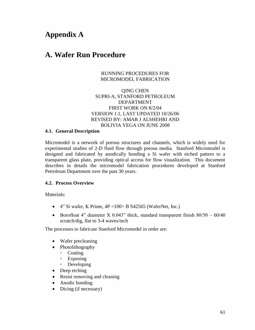
A. Wafer Run Procedure ......................................................................................... 61
4.1. General Description............................................................................................ 61 4.2. Process Overview ............................................................................................... 61 4.3. Photolithography ................................................................................................ 62
x
4.3.1. Photoresist Coating ..................................................................................... 62
4.3.2. Exposure ..................................................................................................... 62 4.3.3. Developing .................................................................................................. 62
4.4. Deep Etching ...................................................................................................... 63
4.5. Post-check .......................................................................................................... 63 4.5.1. Using a microscope: .................................................................................... 63 4.5.2. Using Tencor P2 Profilometer: ................................................................... 63 4.5.3. Using Zygo 3D Surface Profiler: ................................................................ 63
4.6. Resist Removal and Cleaning ............................................................................ 64
4.7. Anodic Bonding ................................................................................................. 64 B. Image Analysis Code ......................................................................................... 66

xi
xii
List of Tables
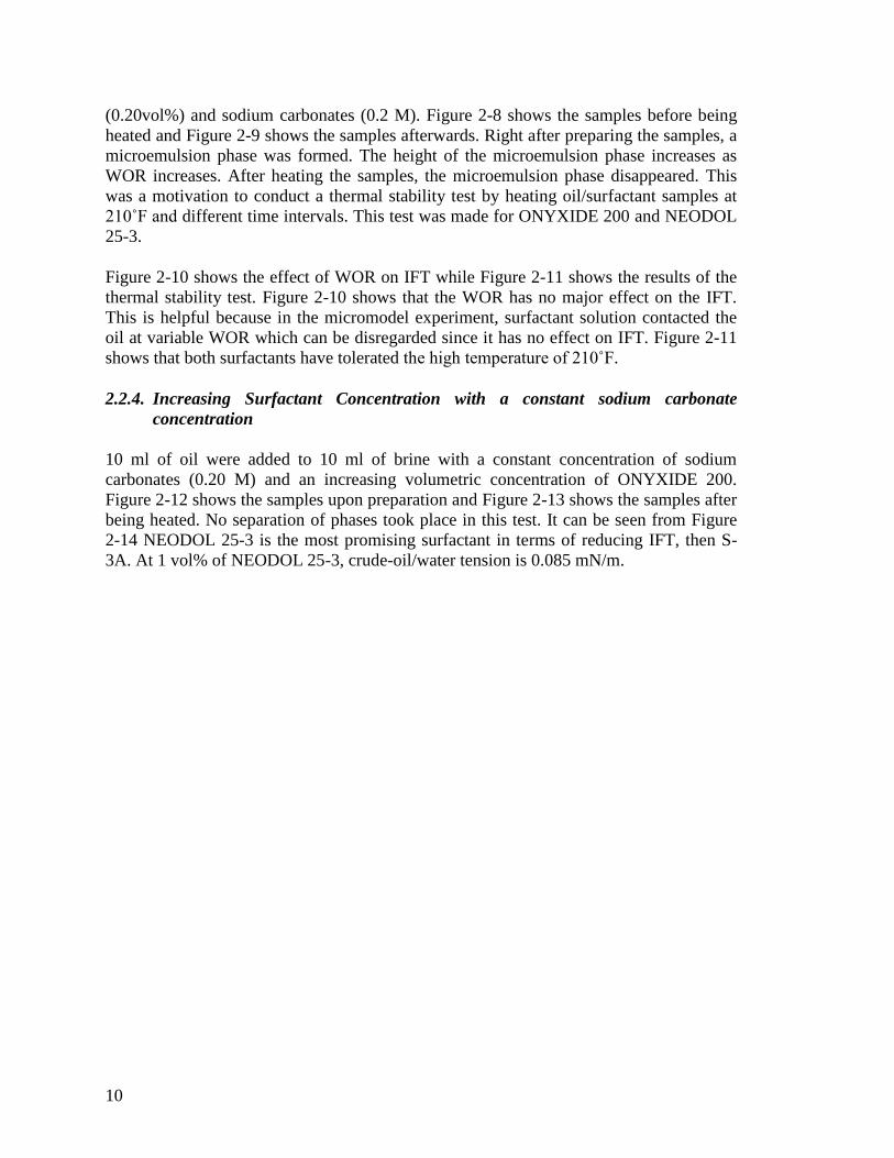
Table 2-1: Brine composition. .......................................................................................... 11
Table 2-2: New brine composition. .................................................................................. 11
Table 3-1: Permeability calculations of mask 2 micromodels. ......................................... 28
Table 3-2: Bond number calculations for the vertical experiment. .................................. 29

xiii
xiv
List of Figures
Figure 2-1: Tensiometer used for measuring IFT. ............................................................ 12
Figure 2-2: Samples made of oil/brine with increasing concentration of sodium
carbonates before being heated. ........................................................................................ 13
Figure 2-3: Samples made of oil/brine with increasing concentration of sodium
carbonates after being heated. ........................................................................................... 13
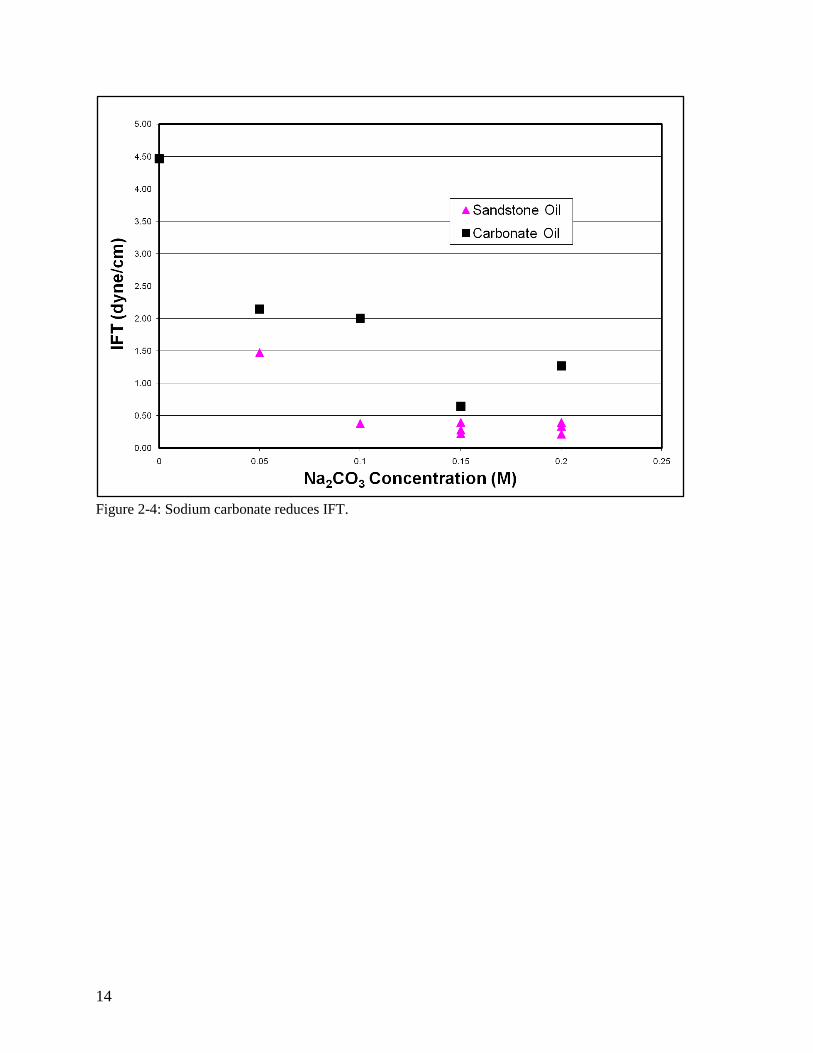
Figure 2-4: Sodium carbonate reduces IFT. ..................................................................... 14
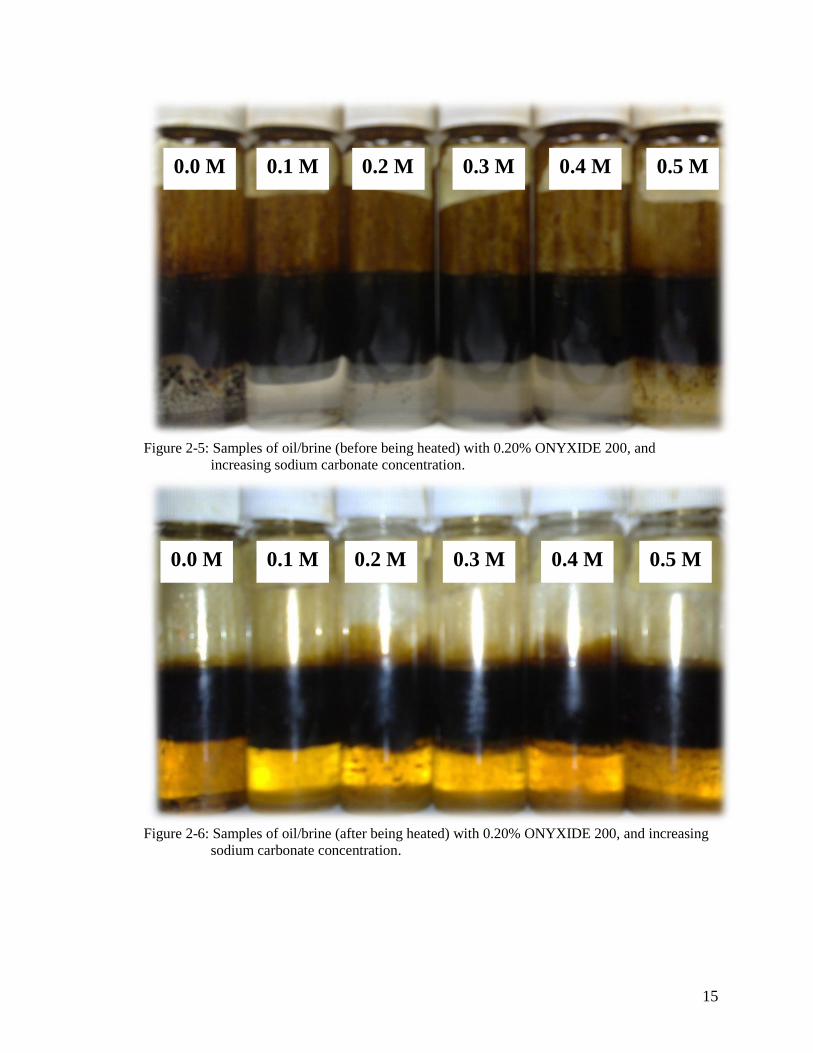
Figure 2-5: Samples of oil/brine (before being heated) with 0.20% ONYXIDE 200, and
increasing sodium carbonate concentration. ..................................................................... 15
Figure 2-6: Samples of oil/brine (after being heated) with 0.20% ONYXIDE 200, and
increasing sodium carbonate concentration. ..................................................................... 15
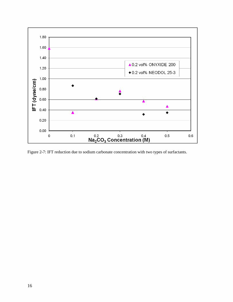
Figure 2-7: IFT reduction due to sodium carbonate concentration with two types of
surfactants. ........................................................................................................................ 16
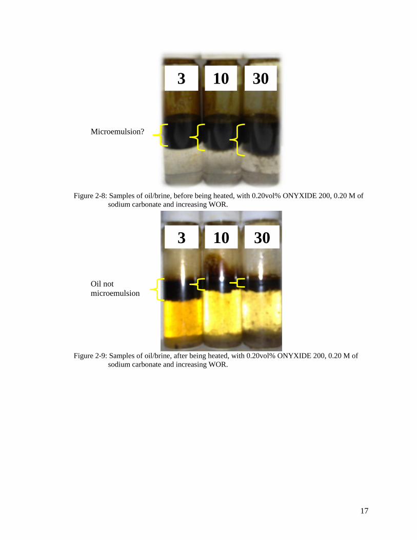
Figure 2-8: Samples of oil/brine, before being heated, with 0.20vol% ONYXIDE 200,
0.20 M of sodium carbonate and increasing WOR. .......................................................... 17
Figure 2-9: Samples of oil/brine, after being heated, with 0.20vol% ONYXIDE 200, 0.20
M of sodium carbonate and increasing WOR. .................................................................. 17
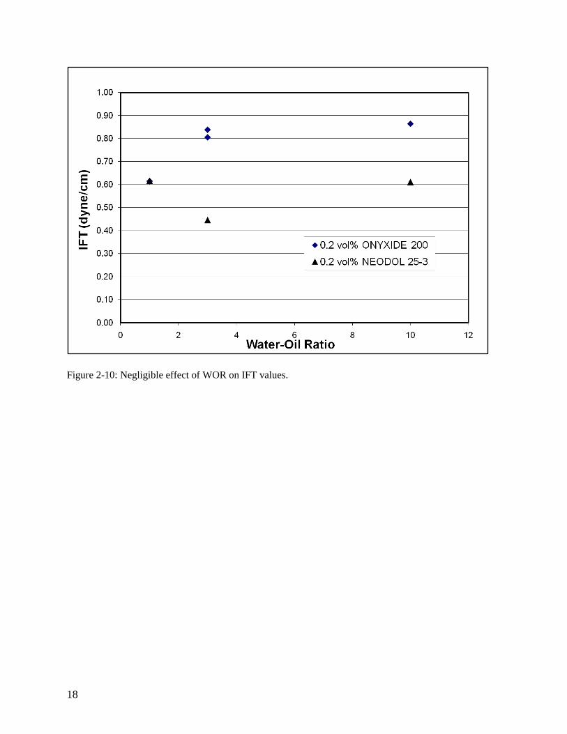
Figure 2-10: Negligible effect of WOR on IFT values. .................................................... 18
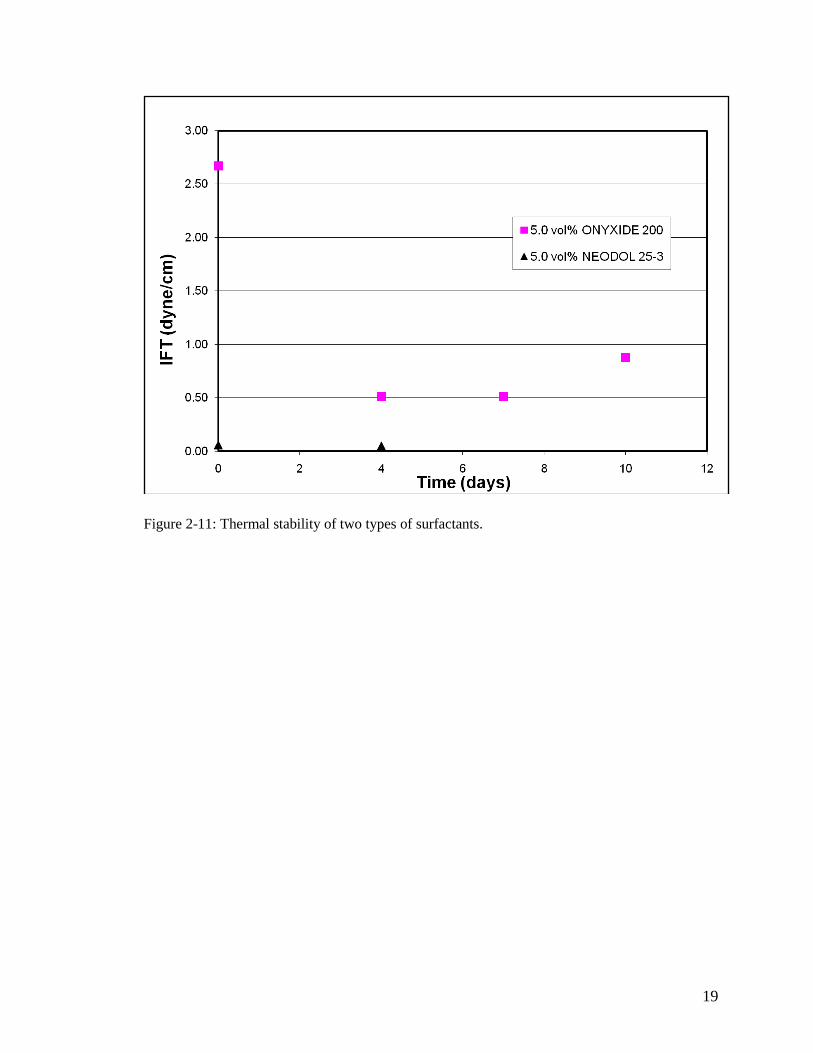
Figure 2-11: Thermal stability of two types of surfactants. .............................................. 19
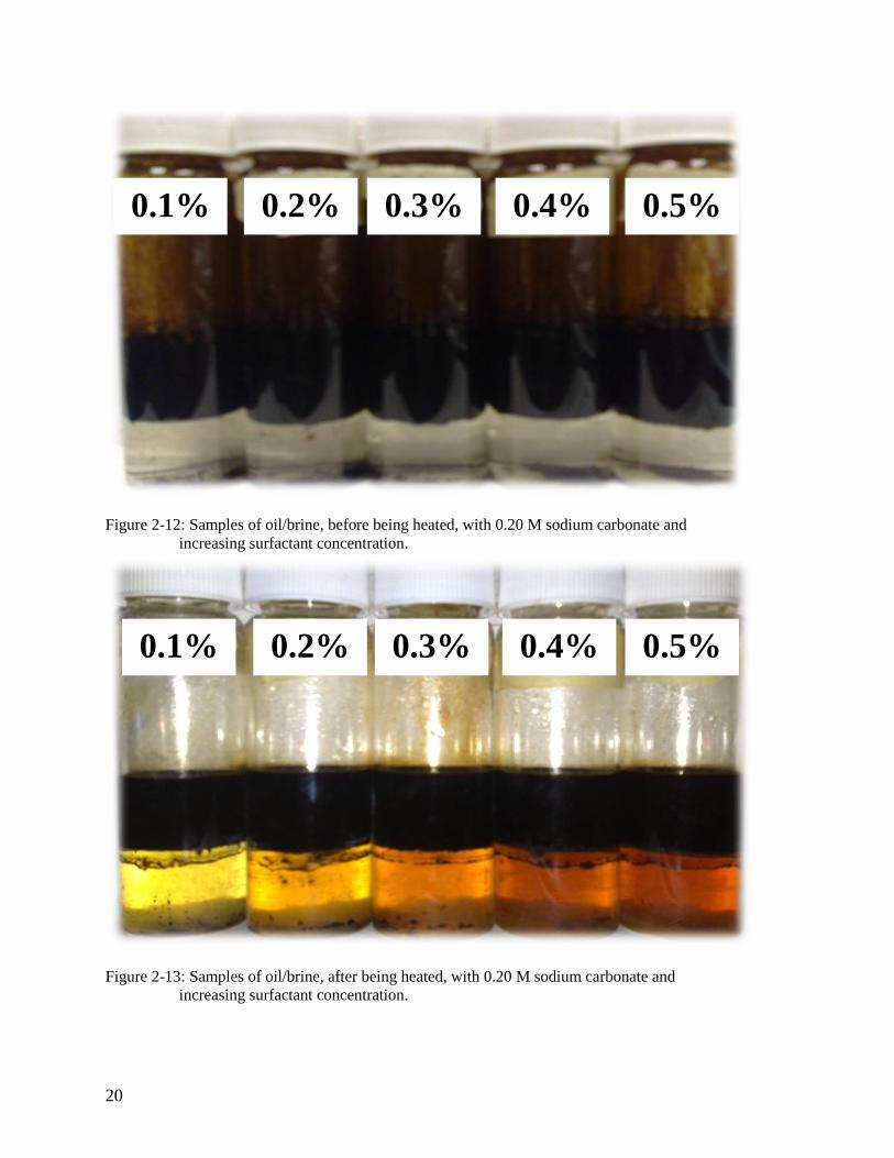
Figure 2-12: Samples of oil/brine, before being heated, with 0.20 M sodium carbonate
and increasing surfactant concentration. ........................................................................... 20
Figure 2-13: Samples of oil/brine, after being heated, with 0.20 M sodium carbonate and
increasing surfactant concentration................................................................................... 20
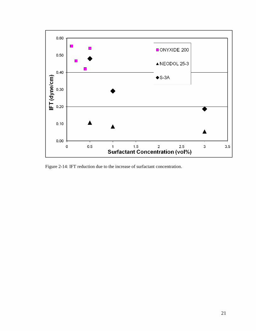
Figure 2-14: IFT reduction due to the increase of surfactant concentration. .................... 21
Figure 3-1: Repeated square pattern in mask 1 (Inwood 2008). ....................................... 30
Figure 3-2: Repeated pattern in mask 2. ........................................................................... 31
Figure 3-3: Bonding apparatus (Hornbrook 1991). .......................................................... 32
Figure 3-4: A typical micromodel (Inwood 2008). ........................................................... 33
Figure 3-5: Schematic of apparatus. ................................................................................. 34
xv
Figure 3-6: The micromodel holder (Inwood 2008). ........................................................ 35
Figure 3-7: 25 microscopic images are obtained (Inwood 2008). .................................... 36
Figure 3-8: 200X microscopic image after the oil flood................................................... 37
Figure 3-9: 200X microscopic image after the 5% filtered S-3A flood. .......................... 38
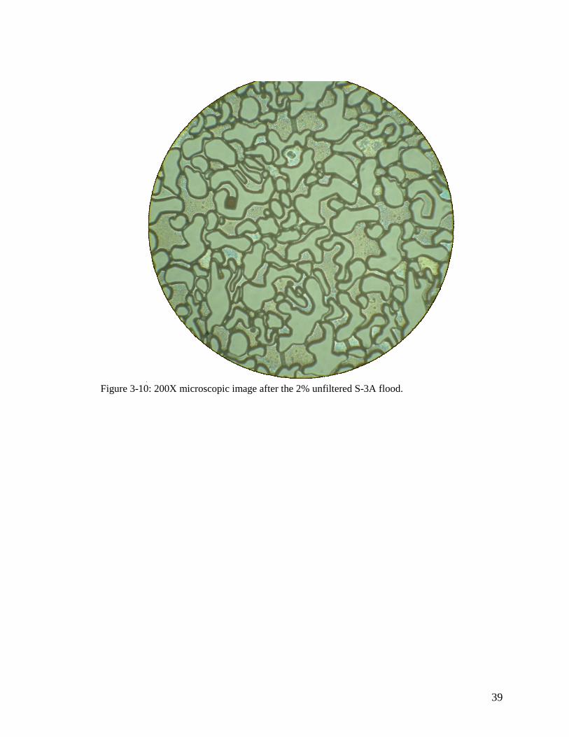
Figure 3-10: 200X microscopic image after the 2% unfiltered S-3A flood. .................... 39
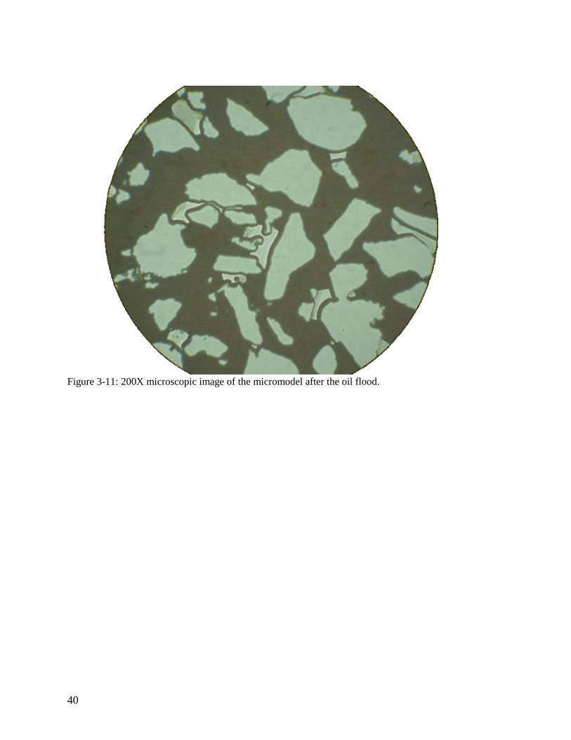
Figure 3-11: 200X microscopic image of the micromodel after the oil flood. ................. 40
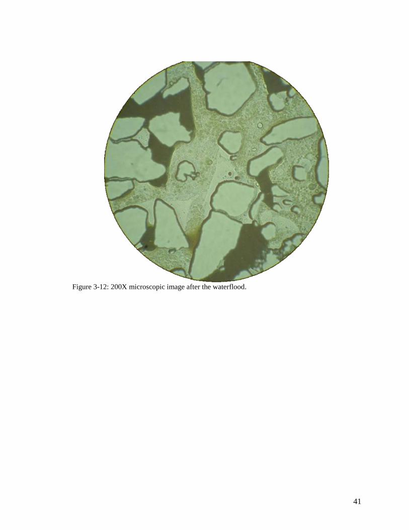
Figure 3-12: 200X microscopic image after the waterflood. ............................................ 41
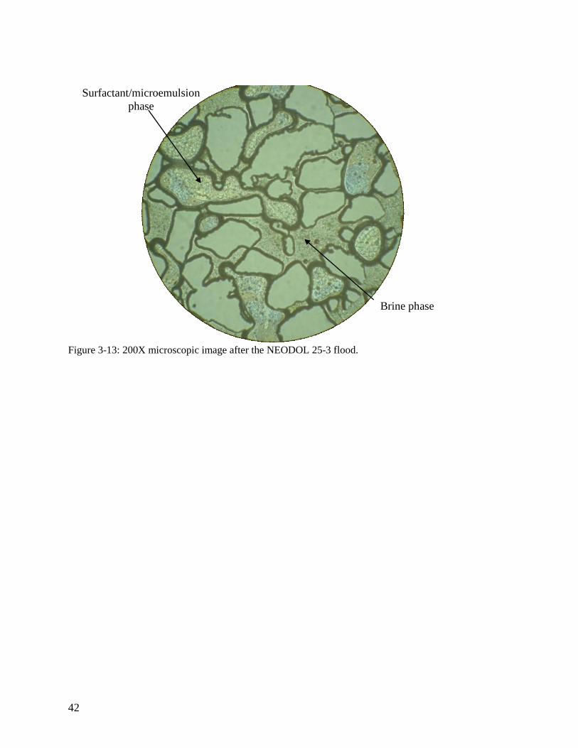
Figure 3-13: 200X microscopic image after the NEODOL 25-3 flood. ........................... 42
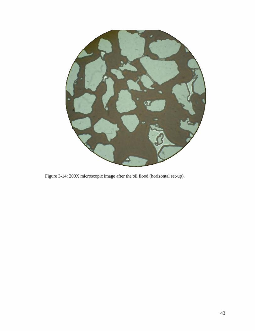
Figure 3-14: 200X microscopic image after the oil flood (horizontal set-up). ................. 43
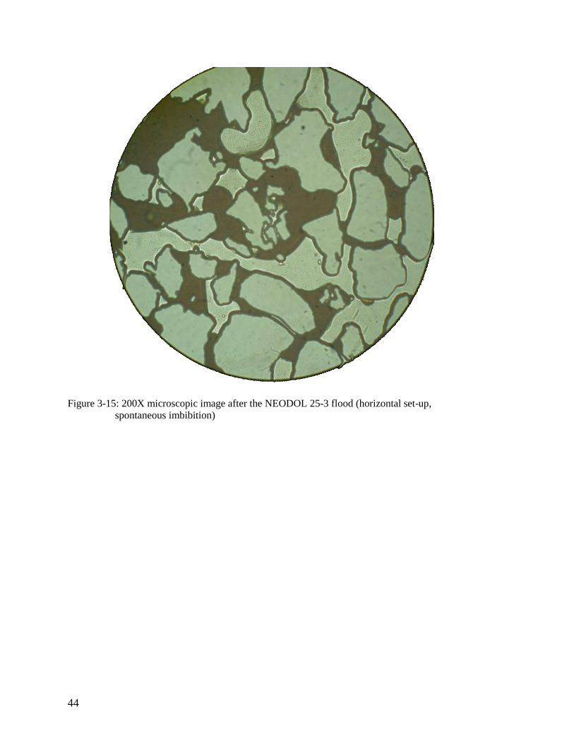
Figure 3-15: 200X microscopic image after the NEODOL 25-3 flood (horizontal set-up,
spontaneous imbibition) .................................................................................................... 44
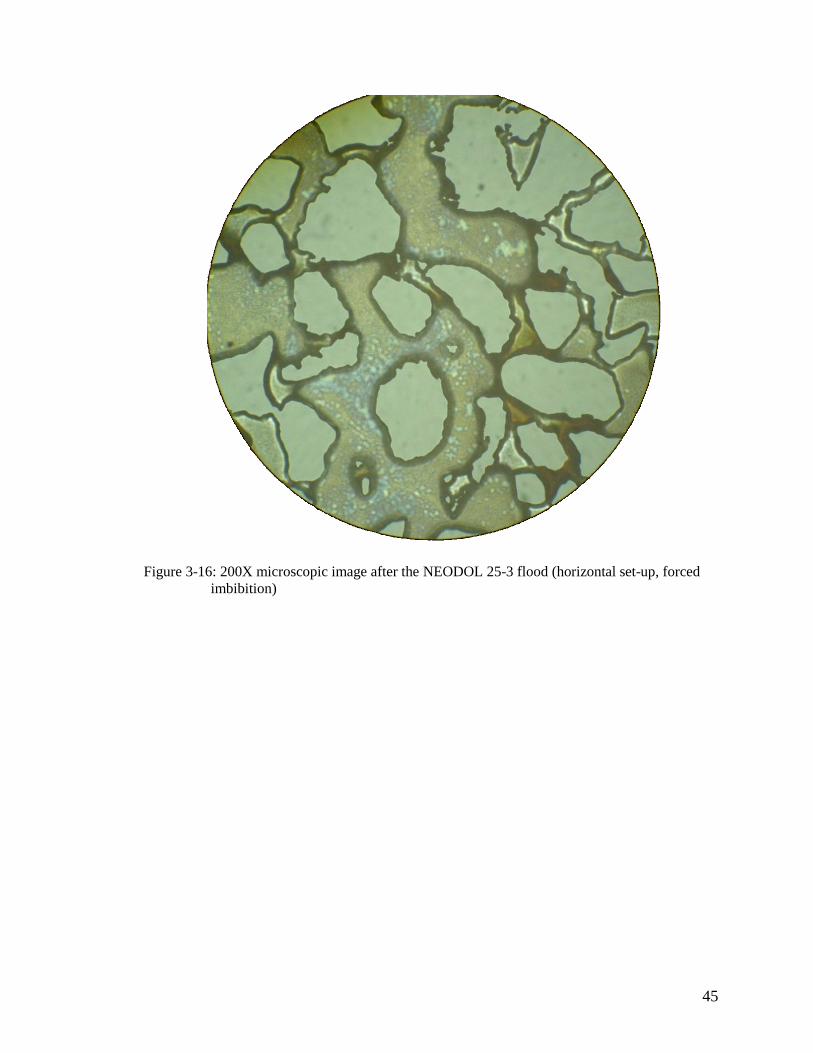
Figure 3-16: 200X microscopic image after the NEODOL 25-3 flood (horizontal set-up,
forced imbibition) ............................................................................................................. 45
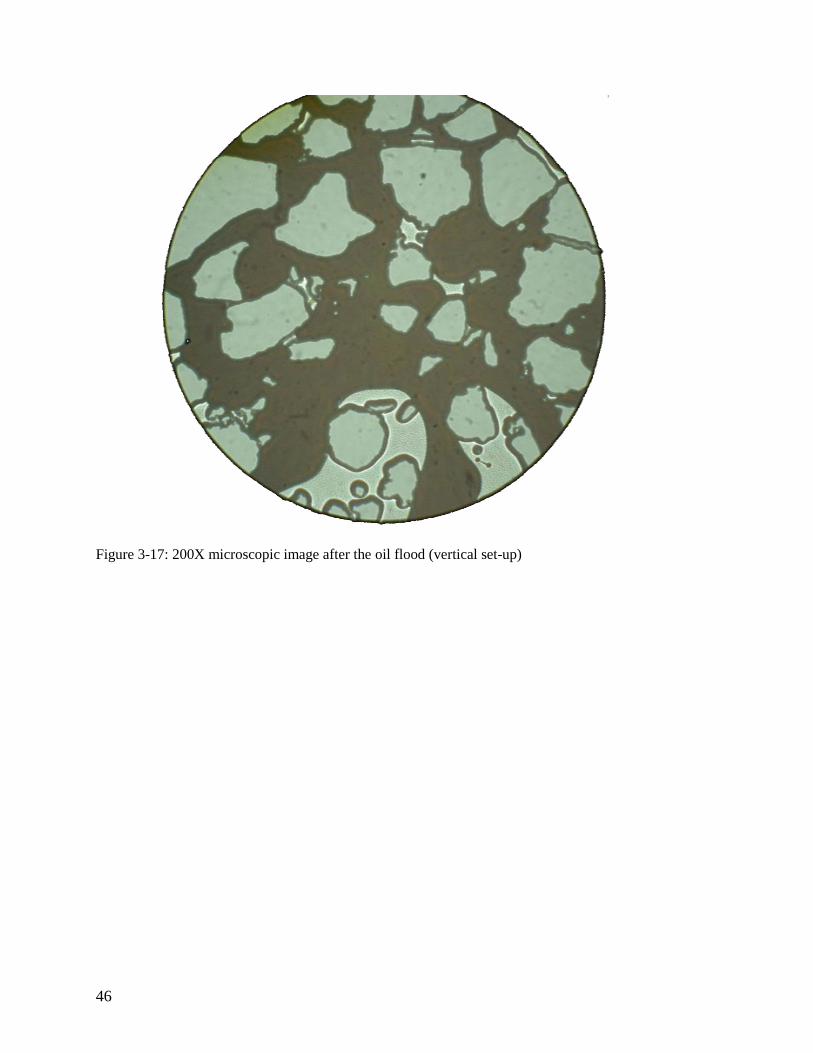
Figure 3-17: 200X microscopic image after the oil flood (vertical set-up) ...................... 46
Figure 3-18: 200X microscopic image after the oil flood (vertical set-up, spontaneous
imbibition)......................................................................................................................... 47
Figure 3-19: 200X microscopic image after the oil flood (vertical set-up, forced
imbibition)......................................................................................................................... 48
Figure 3-20: 200X microscopic image after the oil flood (Experiment IV) ..................... 49
Figure 3-21: 200X microscopic image after the waterflood (Experiment IV) ................. 50
Figure 3-22: 200X microscopic image after the NEODOL 25-3 flood at a low rate
(Experiment IV) ................................................................................................................ 51
Figure 3-23: 200X microscopic image after the NEODOL 25-3 flood at the regular flow
rate (Experiment IV) ......................................................................................................... 52

1
Chapter 1
1. Introduction
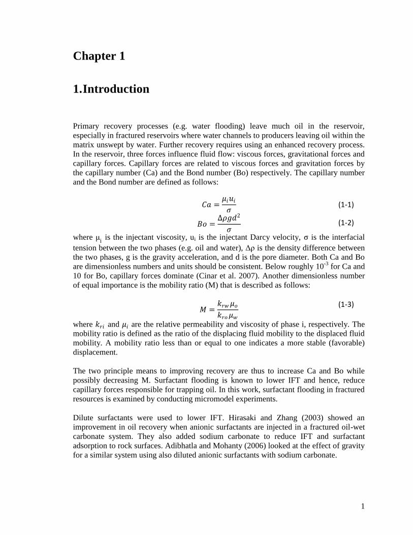
Primary recovery processes (e.g. water flooding) leave much oil in the reservoir,
especially in fractured reservoirs where water channels to producers leaving oil within the
matrix unswept by water. Further recovery requires using an enhanced recovery process.
In the reservoir, three forces influence fluid flow: viscous forces, gravitational forces and
capillary forces. Capillary forces are related to viscous forces and gravitation forces by
the capillary number (Ca) and the Bond number (Bo) respectively. The capillary number
and the Bond number are defined as follows:
𝐶𝑎 =𝜇𝑖𝑢𝑖𝜎
(1-1)
𝐵𝑜 =Δ𝜌𝑔𝑑2
𝜎 (1-2)
where μi is the injectant viscosity, ui is the injectant Darcy velocity, σ is the interfacial
tension between the two phases (e.g. oil and water), Δρ is the density difference between
the two phases, g is the gravity acceleration, and d is the pore diameter. Both Ca and Bo
are dimensionless numbers and units should be consistent. Below roughly 10-3
for Ca and
10 for Bo, capillary forces dominate (Cinar et al. 2007). Another dimensionless number
of equal importance is the mobility ratio (M) that is described as follows:
𝑀 =
𝑘𝑟𝑤𝜇𝑜𝑘𝑟𝑜𝜇𝑤
(1-3)
where 𝑘𝑟𝑖 and 𝜇𝑖 are the relative permeability and viscosity of phase i, respectively. The
mobility ratio is defined as the ratio of the displacing fluid mobility to the displaced fluid
mobility. A mobility ratio less than or equal to one indicates a more stable (favorable)
displacement.
The two principle means to improving recovery are thus to increase Ca and Bo while
possibly decreasing M. Surfactant flooding is known to lower IFT and hence, reduce
capillary forces responsible for trapping oil. In this work, surfactant flooding in fractured
resources is examined by conducting micromodel experiments.
Dilute surfactants were used to lower IFT. Hirasaki and Zhang (2003) showed an
improvement in oil recovery when anionic surfactants are injected in a fractured oil-wet
carbonate system. They also added sodium carbonate to reduce IFT and surfactant
adsorption to rock surfaces. Adibhatla and Mohanty (2006) looked at the effect of gravity
for a similar system using also diluted anionic surfactants with sodium carbonate.
2
In this work, dilute surfactants with sodium carbonates are injected in a micromodel to
visualize the improvement of oil recovery in the presence of gravity. Micromodels are
made of silicon wafers. The pore network, obtained from an image of a rock thin section,
is etched into the wafer. The micromodel is then bonded to glass creating a two-
dimensional porous medium. Silicon micromodels are water wet as a result of the
bonding process.
Surfactant solutions are injected at one side of the micromodel and monitored optically as
they propagate through the micromodel pore network. Reducing capillary forces
minimizes their effect on trapping oil at the pore scale. Hence, buoyancy forces become
dominant and gravity segregates oil and water. Vertical micromodel experiments are
conducted to measure the effect of gravity on oil recovery at low IFT values.
Before conducting the micromodel experiments, a full characterization of
surfactant/brine/oil interactions is obtained. Phase separation tests are conducted to study
the effect of sodium carbonates and surfactant concentration on samples made of brine
and oil. Next, a brief literature review is given. The review is followed by fluid
characterization and experimental details. The major experimental findings are conveyed
by micromodel images. Discussion and conclusions complete the thesis.
1.1. Literature Review
In this work, micromodel experiments are conducted to investigate the improvement in
oil recovery at low interfacial tensions (IFT). Surfactants are used to achieve low IFT
along with sodium carbonate to lower adsorption and alter wettability towards water
wetness. Sodium carbonates are added to the brine as alkali. They increase the negative
charge on rock surfaces making them more water wet. Sodium carbonates are also used
to lower surfactant adsorption to rock surfaces. This section provides a set of relevant
work found in the literature.
1.1.1. Fluid Characterization
Hirasaki and Zhang (2003) looked at surfactant flooding in fractured, oil-wet, carbonate
formations. In such systems, waterflood leads to low recovery as water flows through
fractures leaving oil within the matrix. Moreover, rocks retain oil due to capillary forces
and because carbonates have prominent irregularities (more surface area), much oil
remains. In their work, they studied improvement of oil recovery when using anionic
surfactants and sodium carbonates as alkali. Sodium carbonates were chosen as alkali for
several reasons. For example, they alter wettability towards water-wetness, lower
surfactant adsorption, and produce natural surfactants when reacting with crude oil.
Surfactants and sodium carbonates were characterized by looking at the effect of sodium
carbonate concentration on a brine/oil system, sodium carbonate concentration on a
surfactant solution/oil system, and water-oil ratio (WOR) on a surfactant solution/oil
system with a constant concentration of sodium carbonates (Hirasaki & Zhang, 2003).
3
On another study, Adibhatla and Mohanty (2006) conducted core-flooding experiments
and numerical simulations to investigate a surfactant-aided gravity drainage process.
They also used anionic surfactants, specifically alkyl ethoxylated surfactants, to lower the
IFT. Before conducting the experiment, they followed a surfactant screening procedure
proposed by Seethepalli et al (2004). Surfactants were screened based on phase behavior
of samples made of oil/diluted surfactants with varying sodium carbonate concentration,
IFT values, and wettability; a similar screening methodology was also implemented by
Seethepalli et al. It was found that sodium carbonate concentration has to be at an
optimum value to give the greatest reduction in IFT. Moreover, the wettability of oil wet
surfaces was altered to intermediate to moderate water wet. These two factors: the IFT
reduction and the wettability alteration towards water wetness led to an increase in oil
recovery to about 60% in 60 days.
Levitt et al. (2006) proposed another screening methodology of chemical EOR fluids.
The screened fluids include surfactants, polymers, co-surfactants and co-solvents. It was
found that increasing the length of the hydrophopic part of the surfactants improves its
performance in terms of higher solubilization ratio and lower optimum salinity.
Propylene oxide (PO), a hydrophobic functional group, is added to the surfactant at
different concentrations. Three types of surfactants were investigated: C16-17-(PO)3-
SO4, C16-17-(PO)5-SO4 and C16-17-(PO)7-SO4 along with three types of co-
surfactants: alcohol propoxy sulfate (APS), C15-18 internal olefin sulfonate (IOS) and
C20-24 alpha olefin sulfonate (AOS). The fluids are evaluated by conducting phase
behavior tests at different temperatures on samples made of surfactant/oil/brine. The
testing criteria include the high stability and the low viscosity of the microemulsion
phase, and the great reduction in the interfacial tension (IFT). It was found that C15-18
IOS with the 7 PO surfactant is the optimum mixture for low temperature dolomite
reservoirs. For high temperatures (above 60˚C), IOS hydrolyzes and sulfonate co-
surfactants (e.g. AOS) are recommended. The researchers also concluded that adding
sodium carbonate lowers IFT even more and reduces equilibration time.
Wellington and Richardson worked on designing surfactant flooding systems to obtain
the greatest possible oil recovery using 40 anionic, 25 cationic, and 120 surfactant
combinations. To maximize the recovery, surfactant concentration is kept at an optimum
value at which oil and water phases are solely present with no microemulsion phase.
Moreover, the mobility of the surfactant flood is kept below oil mobility by injecting
polymer, to enhance displacement efficiency. Surfactants were screened based on cloud
point, the “maximum temperature at which a single-phase solution exists,” and IFT
measurements. It was found that the optimum concentration, for the examined
surfactants, is about 0.4wt%. With such concentration, about one pore volume of
surfactant solution is effective in displacing all residual oil in sand packs with less than
0.1 pore volume of surfactant loss. Moreover, it was found that the amount of
undisplaced oil increases with loss of surfactants in a surfactant flood. Hence, adsorption
control is highly recommended in designing surfactant flooding processes (Wellington &
Richardson, 1997). Osterloh and Jante used polyethylene glycol (PEG) additives to lower
adsorption of a surfactant/polymer system. By conducting core-flooding experiments,
4
they concluded that PEG-1000 has lowered adsorption the most compared to the other
glycols (Osterloh & Jante, 1992).
Gupta and Mohanty looked at the effect of temperature on a surfactant flooding process
in a carbonate system. It was found that increasing the temperature causes the rock matrix
to become more water wet which was also reported by Wang and Gupta (1995),
Hamouda and Gomari (2006), Schembre et. al. (2006), and Hjelmeland and Larronda
(1986). Hence, oil recovery increases as temperature increases in surfactant flooding. The
wettability alteration towards water wetness by an increase in temperature is interpreted
by two reasons. The first is adsorption of crude oil components to the solid surface
causing the surface to become more oil wet decreases as temperature increases. Another
reason is that the activity of calcium ions on the solid surface also decreases with an
increase in temperature. (Gupta & Mohanty, 2007).
1.1.2. Micromodel Experiments
Micromodels are two-dimensional systems that consist of an etched silicon wafer bonded
to a glass wafer. The silicon wafer can be etched with any desired network. An inherent
limitation in micromodels comes from the fact that they are two dimensional and more
care should be taken in extrapolating the experimental results to the three-dimensional
space. However, they provide an excellent means of optically visualizing displacement
mechanisms and interactions of injected phases at a representative pore scale.
Feng et al. in 2004 conducted micromodel experiments to study water-alternating gas
(WAG) displacement mechanisms. They found that WAG displacement mechanisms
differ than water-oil or gas-oil displacement mechanisms. Oil becomes an intermediate
phase between water, occupying small pores, and gas, occupying large pores (in a water-
wet micromodel). Expansion of gas helps displace oil. Such realization had to be
visualized, by conducting a micromodel experiment (Feng et al. 2004).
Rangel-German and Kovscek (2006) conducted micromodel experiments to investigate
matrix-fracture transfer mechanisms of two phases. The wafers were etched with a
representative Berea sandstone pore network (matrix) with two channels on two opposite
sides of the network (fractures). The experiments were conducted by injecting the wetting
phase (water) into the fracture and visualizing how it imbibes into the matrix. They
showed that imbibition of wetting phase into the matrix is proportional to the volume of
injected water at low injection rates and proportional to the square root of time at high
flow rates. These results were concluded by microscopically monitoring the transient
imbibition process.
The paper by Riaz et al (2007) showed the importance of M to fluid dynamics by
monitoring core-flooding experiments with a CT scanner and conducting numerical
simulations. Their work demonstrated how M is directly related to the stability of the
injectant. Aktas et al (2008) and Buchgraber et al (2009) show how to modify M towards
a more stable front by injecting associative polymers. They used micromodels similar to
those ones described above. Associative polymers are used to lower the mobility of the
5
injectant and the overall mobility ratio. They showed that injecting associative polymers
stabilizes the displacement front and thereby improving oil recovery. The experiments
were conducted on two-dimensional silicon micromodels similar to the ones used by
Rangel-German and Kovscek (2006). The aqueous phase of the associative polymers was
forcedly imbibed into the micromodel from one side and the recovered oil was collected
from the other side (Aktas et al. 2008).
Silicon and glass micromodels are naturally water wet. To make them oil wet, they are
treated with hexadecyltrimethylammonium bromide (Hirasaki & Zhang, 2003).

7
Chapter 2
2. Fluid Characterization
A phase behavior study was carried out similar to the study of Hirasaki and Zhang
(2003). Four tests were conducted by preparing samples of oil/brine/dilute surfactant to
study the effect on IFT of the following:
Increasing sodium carbonate concentration without surfactants
Increasing sodium carbonate concentration at a constant surfactant concentration
Increasing water-oil ratio (WOR) at a constant surfactant and sodium carbonate
concentrations
Increasing surfactant concentration at a constant sodium carbonate concentration
The IFT measurements were obtained using a spinning drop tensiometer. The following
section presents the surfactants that were included in the study along with a brief
description of the spinning drop tensiometer. The results of the phase behavior tests are
discussed afterwards.
2.1. Surfactant Screening
In this work, three surfactants were evaluated based on their interfacial tension reduction
(IFT): ONYXIDE 200 and PETROSTEP S-3A from STEPAN and NEODOL 25-3 from
Shell Chemical.
ONYXIDE 200 is composed of 78.5% 1,3,5-Triazine-1,3,5(2H,4H,6H)-triethanol and
21.5% water (78.5% active). ONYXIDE 200 has the following properties:
Flash Point: > 201˚F
Boiling Point: 212˚F
Density: 1.15 g/ml
Percent Volatile (% w/w): 21.5
pH: 10.5 (as is)
Solubility in Water: Miscible (STEPAN, 2006)
PETROSTEP S-3 A is an internal olefin sulfonate (60.72% active). It has the following
properties:
Appearance @ 70 F: Brown liquid
Flash Point: > 201˚F
Boiling Point: >212˚F
Density: 8.6 lb/gal
8
Percent Volatile (% w/w): 35
pH: 10-11.5 (10% aqueous)
Solubility in Water: soluble (STEPAN, 2006)
NEODOL 25-3 (100% active) is made of ethylene oxide and pure C12-C15 NEODOL
alcohol with a 3:1 molar ratio respectively. NEODOL 25-3 has the following properties:
Flash Point: 325˚F
Pour Point: 41˚F
Density: 0.908 g/ml
Kinematic Viscosity (@40˚C): 17 cSt (ShellChemicals, 2006)
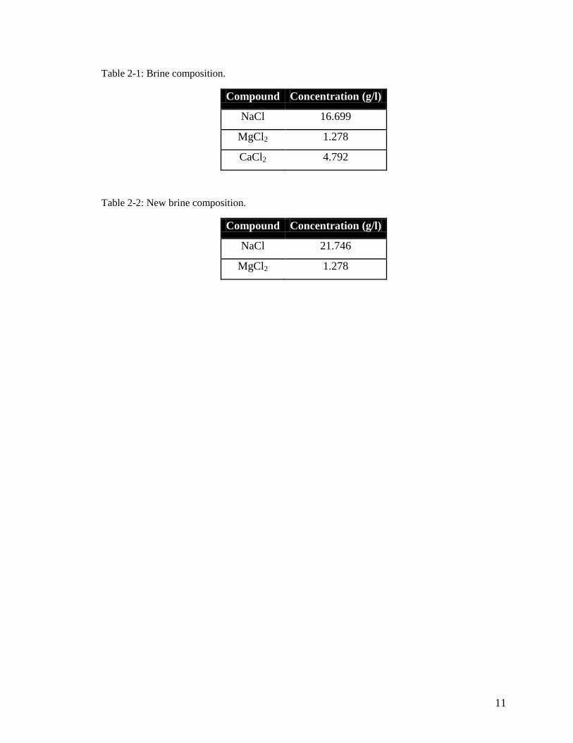
The IFT was measured using a spinning drop tensiometer shown on Figure 2-1. The basic
principle of a tensiometer is measuring the width of an elongated oil drop submersed in a
brine/surfactant solution. Both the oil drop and the brine are injected by a syringe into a
capillary tube. The tube is placed inside the tensiometer and rotated about the
longitudinal axis. The following formula is used to calculate the IFT (σ)
𝜎 =1
4Δ𝜌𝜔2𝑟3 (2-1)
Where Δρ is the density difference between oil and brine/surfactant solution in kg
m3, r is
the elongated oil drop radius in meters and
ω =2π
f1000
with f as the angular velocity read from the tensiometer in msec
shaft rev. The measurements
were obtained for oil/brine systems with different surfactant concentrations. It has to be
noted that the capillary tubes have to be cleaned before usage. They are flushed with
decane followed by acetone.
2.2. Phase Behavior Tests
This work is different than previous works discussed in the literature. It studies pore level
displacement mechanisms with surfactant flooding by conducting micromodel
experiments. A fracture is simulated by injecting along one side of the micromodel and
allowing spontaneous imbibition to occur. Experiments are also conducted vertically to
see the effect of gravity at low IFT values.
There are three types of fluids in this work: brine, oil, and surfactant. Brine is composed
of sodium chloride, magnesium chloride, and calcium chloride. Concentrations of these
salts are shown on Table 2-1.
9
Oil was obtained from two different reservoirs: sandstone (27.3˚API) and carbonate
(27.0˚API) reservoirs. Two surfactants are used in this study: ONYXIDE 200 from
Stepan Company and NEODOL 25-3 from Shell Chemical Company.
Four phase separation tests were conducted, similar to those described in the paper by
Hirasaki and Zhang (2003), to study the effect of sodium carbonate concentration, water-
oil ratio, and surfactant concentration. Samples of solutions with oil from a sandstone
reservoir were prepared. The samples were then heated in an oven for a week to a
temperature of 210˚F.
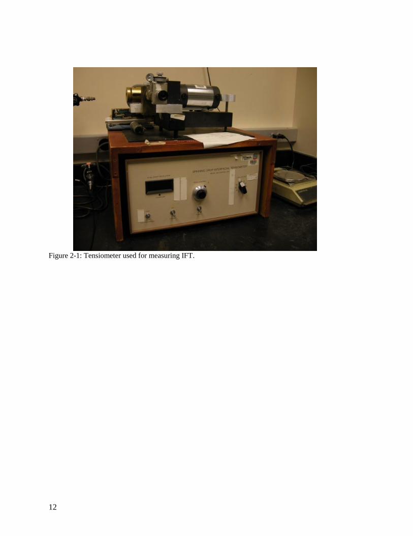
2.2.1. Increasing Sodium Carbonate Concentration
In this test, 10 ml of oil (sandstone and carbonate oil; 5 samples for each) were added to
10 ml of brine with increasing concentration of sodium carbonates. Figure 2-2 shows the
samples before being heated and Figure 2-3 shows the samples after they were taken out
of the oven. White precipitates of calcium carbonates were observed when the samples
were prepared. Most of the precipitates dissolved in the aqueous phase after heating the
samples. However, these precipitates might block the micromodel network pores and
throats and thus calcium chloride was not added to the brine. More sodium chloride was
added to compensate for the chloride ions. The new composition is shown on Table 2-2.
The aqueous phase was yellowish in color after heating the samples. This indicates that
some oil phase components dissolved in the brine. Samples of the brine were centrifuged
at 50 rpm for one hour to see if more than one phase is present in the aqueous phase.
Only one phase is found in the brine.
Figure 2-4 shows the IFT measurements for the samples for both oil types. It can be
clearly seen that increases in sodium carbonate concentration lowers the IFT as
previously suggested by Hirasaki and Zhang (2003).
2.2.2. Increasing Sodium Carbonates Concentration with a Constant Surfactant
Concentration
Samples of 10 ml of sandstone oil were added to 10 ml of brine with a constant
concentration of ONYXIDE 200 (0.20vol%) and an increasing concentration of sodium
carbonates. Less precipitates formed in this test than those formed in the previous one.
The surfactant in the brine helps dissolve the precipitates. Figure 2-5 shows the samples
upon preparation and Figure 2-6 shows the samples after being heated.
Figure 2-7 shows the IFT measurements with two different surfactants. It roughly
observed the same result from the previous test that sodium carbonates lower the IFT.
2.2.3. Increasing Water-Oil Ratios (WOR):
The purpose of this test is to study the effect of increasing WOR on phase separation.
Samples were prepared with brine, a constant concentration of ONYXIDE 200
10
(0.20vol%) and sodium carbonates (0.2 M). Figure 2-8 shows the samples before being
heated and Figure 2-9 shows the samples afterwards. Right after preparing the samples, a
microemulsion phase was formed. The height of the microemulsion phase increases as
WOR increases. After heating the samples, the microemulsion phase disappeared. This
was a motivation to conduct a thermal stability test by heating oil/surfactant samples at
210˚F and different time intervals. This test was made for ONYXIDE 200 and NEODOL
25-3.
Figure 2-10 shows the effect of WOR on IFT while Figure 2-11 shows the results of the
thermal stability test. Figure 2-10 shows that the WOR has no major effect on the IFT.
This is helpful because in the micromodel experiment, surfactant solution contacted the
oil at variable WOR which can be disregarded since it has no effect on IFT. Figure 2-11
shows that both surfactants have tolerated the high temperature of 210˚F.
2.2.4. Increasing Surfactant Concentration with a constant sodium carbonate
concentration
10 ml of oil were added to 10 ml of brine with a constant concentration of sodium
carbonates (0.20 M) and an increasing volumetric concentration of ONYXIDE 200.
Figure 2-12 shows the samples upon preparation and Figure 2-13 shows the samples after
being heated. No separation of phases took place in this test. It can be seen from Figure
2-14 NEODOL 25-3 is the most promising surfactant in terms of reducing IFT, then S-
3A. At 1 vol% of NEODOL 25-3, crude-oil/water tension is 0.085 mN/m.
11
Table 2-1: Brine composition.
Compound Concentration (g/l)
NaCl 16.699
MgCl2 1.278
CaCl2 4.792
Table 2-2: New brine composition.
Compound Concentration (g/l)
NaCl 21.746
MgCl2 1.278
12
Figure 2-1: Tensiometer used for measuring IFT.
13
Figure 2-2: Samples made of oil/brine with increasing concentration of sodium carbonates before
being heated.
Figure 2-3: Samples made of oil/brine with increasing concentration of sodium carbonates after
being heated.
0.00M 0.05M 0.10M 0.15M 0.20M
0.00M 0.05M 0.10M 0.15M 0.20M
14
Figure 2-4: Sodium carbonate reduces IFT.
15
Figure 2-5: Samples of oil/brine (before being heated) with 0.20% ONYXIDE 200, and
increasing sodium carbonate concentration.
Figure 2-6: Samples of oil/brine (after being heated) with 0.20% ONYXIDE 200, and increasing
sodium carbonate concentration.
0.0 M 0.1 M 0.2 M 0.3 M 0.4 M 0.5 M
0.0 M 0.1 M 0.2 M 0.3 M 0.4 M 0.5 M
16
Figure 2-7: IFT reduction due to sodium carbonate concentration with two types of surfactants.
17
Figure 2-8: Samples of oil/brine, before being heated, with 0.20vol% ONYXIDE 200, 0.20 M of
sodium carbonate and increasing WOR.
Figure 2-9: Samples of oil/brine, after being heated, with 0.20vol% ONYXIDE 200, 0.20 M of
sodium carbonate and increasing WOR.
3 10 30
3 10 30
Microemulsion?
Oil not
microemulsion
18
Figure 2-10: Negligible effect of WOR on IFT values.
19
Figure 2-11: Thermal stability of two types of surfactants.
20
Figure 2-12: Samples of oil/brine, before being heated, with 0.20 M sodium carbonate and
increasing surfactant concentration.
Figure 2-13: Samples of oil/brine, after being heated, with 0.20 M sodium carbonate and
increasing surfactant concentration.
0.5% 0.1% 0.2% 0.3% 0.4%
0.1% 0.2% 0.5% 0.4% 0.3%
21
Figure 2-14: IFT reduction due to the increase of surfactant concentration.

22
23
Chapter 3
3. Micromodel Experiments
Micromodels are two-dimensional systems in which an etched silicon wafer is bonded to
a glass wafer. Because micromodels are only two-dimensional, extrapolating results to 3-
dimensional systems has to be done cautiously. Micromodels provide a tool of direct
visualization of fluid interactions when conducting an experiment. The following section
describes the process of fabricating the micromodels then discusses the micromodel
experiments.
3.1. Micromodel Fabrication
The wafers used to make the micromodels are 4” Silicon wafers, K Prime, 4P <100> B
S42565. Two pore networks from two masks: mask 1 and mask 2 were used to make the
micromodels. Each mask contains a 5X5 cm pore network. Mask 1 contains a pore
network similar to a Berea sandstone made from a repeated square pattern shown on
Figure 3-1. The pattern is 490 μm by 400 μm and is repeated 102 times across each side
of the network. Grain sizes range in length from 30 to 300 μm. Porosity is about 47%.
The permeability of mask 1 micromodels was measured by Inwood (2008) and was of the
order of 1 Darcy.
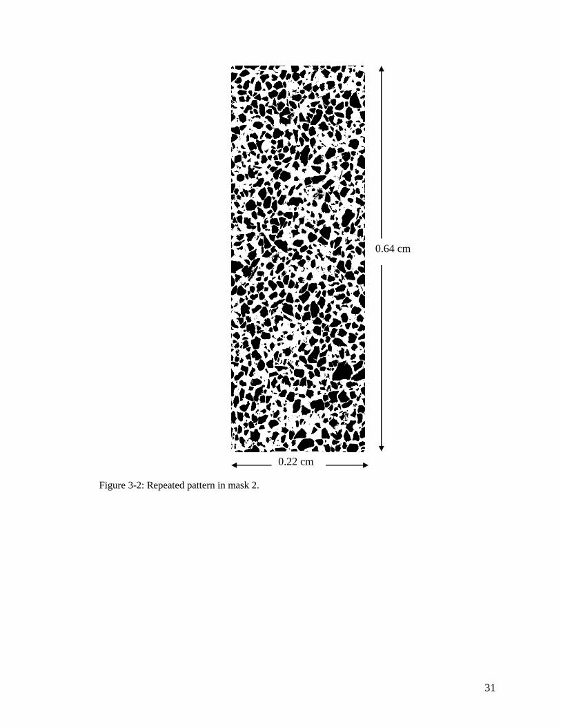
Mask 2 is sandstone with a repeated image shown on
Figure 3-2. The repeated image is 0.22X0.64 cm. The porosity is about 54% with grain
size ranging from 125 to 250 μm in diameter. The permeability of mask 2 micromodels
were measured by injecting distilled water at variable pressures and recording the
corresponding flow rates, and at variable flow rates and recording the corresponding
pressures as shown on Table 3-1. The permeability of the micromodels came out to be
around 3 Darcy.
Most of the steps involved in making the micromodels take place in Stanford
Nanofabrication Facility (SNF), shown in details in Appendix A.A, and they are the
following (Stanford Nanofabrication Facility 2009):
3.1.1. Dehydration:
The wafers are dehydrated in a dehydrating oven for about 30 minutes. Dehydration is
performed at 150˚C and involves priming the wafers with hexamethyldisilazane
(HMDS). The HMDS improves the photoresist adhesion to the wafers.
24
3.1.2. Coating:
The silicon wafers are then coated with Shipley 3612 photoresist in one of the svgcoat
tracks. Shipley 3612 is 1-1.6 μm thick. The following programs are chosen:
Prime program: off
Coat program: program # 8
Prebake program: program # 2
3.1.3. Exposure:
At this step, a mask containing the pore network is needed. A karlsuss aligner is used to
expose the wafers to the mask. A soft contact program with 2.6-seconds exposure time
and 40-μm gap width was selected.
3.1.4. Developing:
The pore network has been transferred to the wafers at this point and they need to be
developed to remove the excessive photoresist. Developing takes place in one of the
svgdev tracks. The following programs are chosen:
Developing program: program # 4
Oven bake: program # 2
3.1.5. Etching:
After developing the wafers, the wafers are taken out from the photolithography area.
They are etched in the stsetch which is an inductive charged plasma etcher. For our case,
we use a deep etching recipe. The input etching time depends on the desired etching
depth. The wafer is etched for a specific time (say 5 minutes). Then, the etched depth is
measured using a microscope, the P2, or the zygo. The etching rate is calculated and then
etching time is chosen. One thing to note about the etcher is that it does not etch
uniformly. It etches the most at the edges. In the micromodels used in this work, the
etching depth is about 30 μm at the middle and 40 μm at the edges.
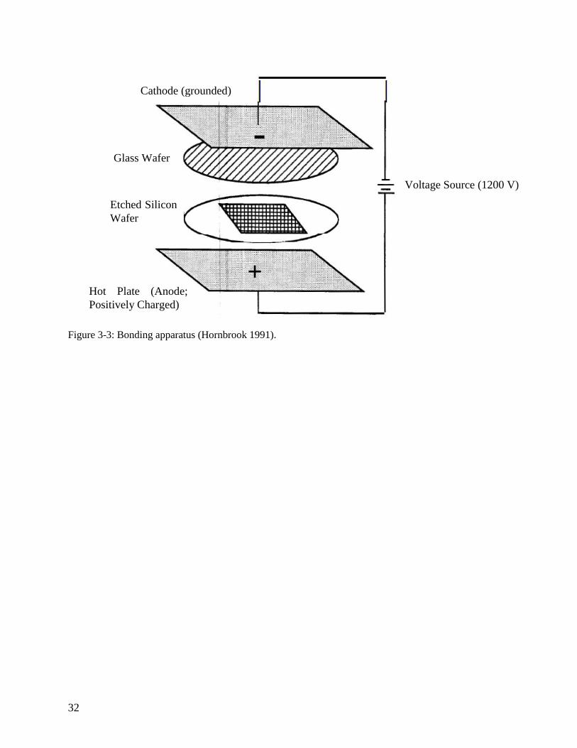
3.1.6. Anodic Bonding:
After etching the wafers, four ports are drilled at the corners of the network in the
Stanford crystal shop. They are then cleaned in the wbsilicide wet bench in the SNF
along with 4” Pyrex glass wafers in a hot bath (120˚F) of 9:1 sulfuric acid:hydrogen
peroxide. The silicon wafers are anodically bonded with the glass wafers under 1200
volts. The bonding apparatus consists of a hot plate, a voltage source, and a voltage plate.
The hot plate is connected to the positive voltage source and the voltage plate is
grounded. The etched silicon wafer is heated by itself for 45 minutes on the hot plate at a
temperature of 350˚C. the wafer is then dusted to ensure that no particles reside on it.
After that, a clean glass wafer is placed on top of the silicon wafer for two minutes. The
25
temperature is then reduced to 300˚C and the voltage plate is placed on top of the glass
wafer as shown on Figure 3-3. It is recommend to apply evenly distributed weight on the
voltage plate. After that, the voltage source is turned on for 50 minutes to have a
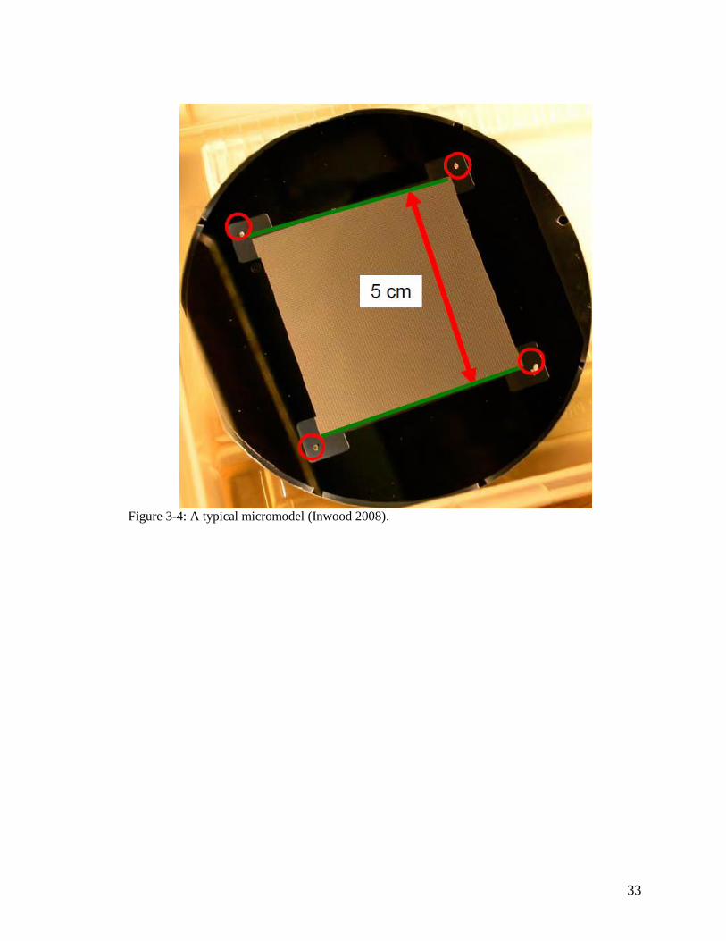
complete bonding (Hornbrook 1991). Figure 3-4 shows a micromodel with the four ports
(surrounded by the red circles), two fractures (shown by the solid green lines), and the
5X5 cm pore network.
3.2. Experimental Setup
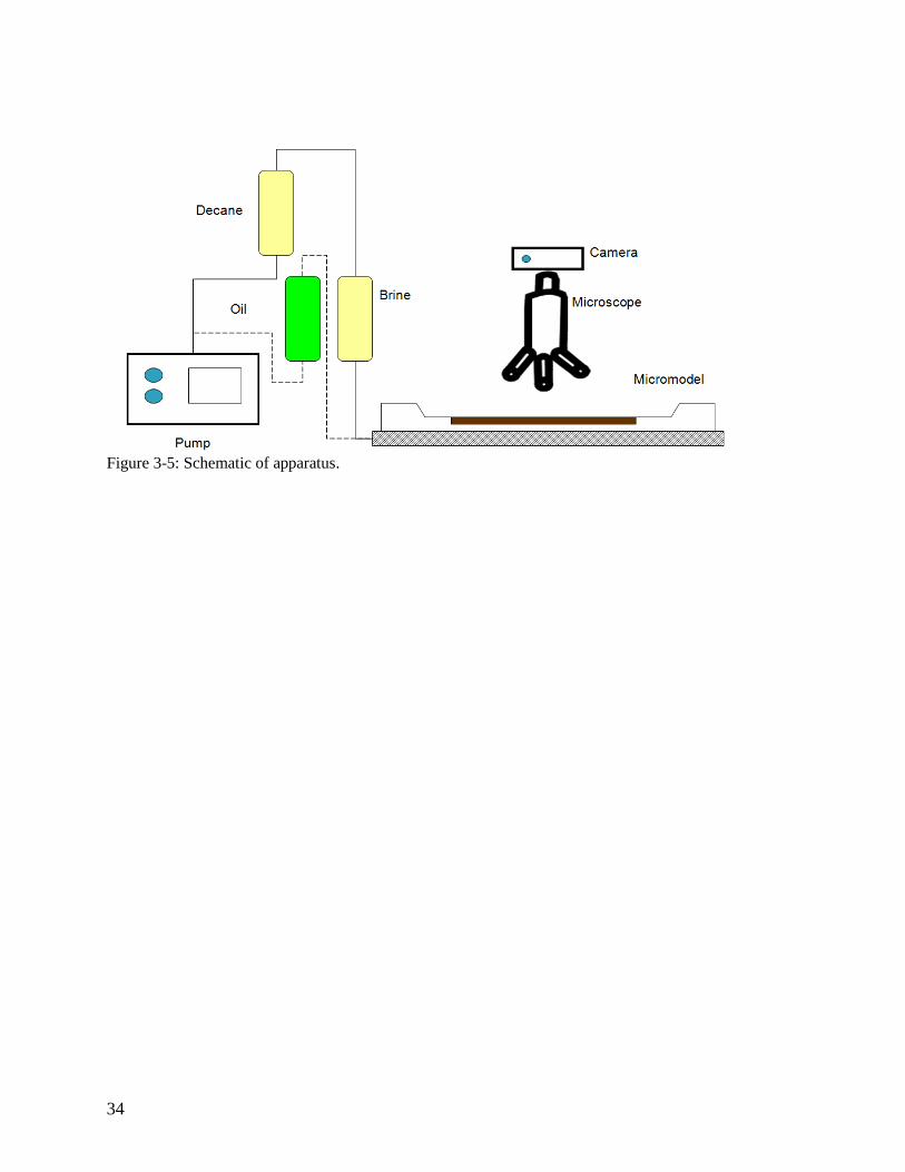
Figure 3-5 shows the schematic of the main components in the experiments. The injection
part is made of a syringe pump that is filled with distilled water. The pump is connected
by plastic tubes to bombs filled with the injectants. The tubes are connected to the bottom
of the bombs if they carry the heavier fluid and to the top if they carry the lighter fluid.
The data gathering part consists of a microscope and a camera. The microscope is Nikon
Eclipse ME 600 (reflected light) with 40X, 100X, and 200X magnifications. The camera
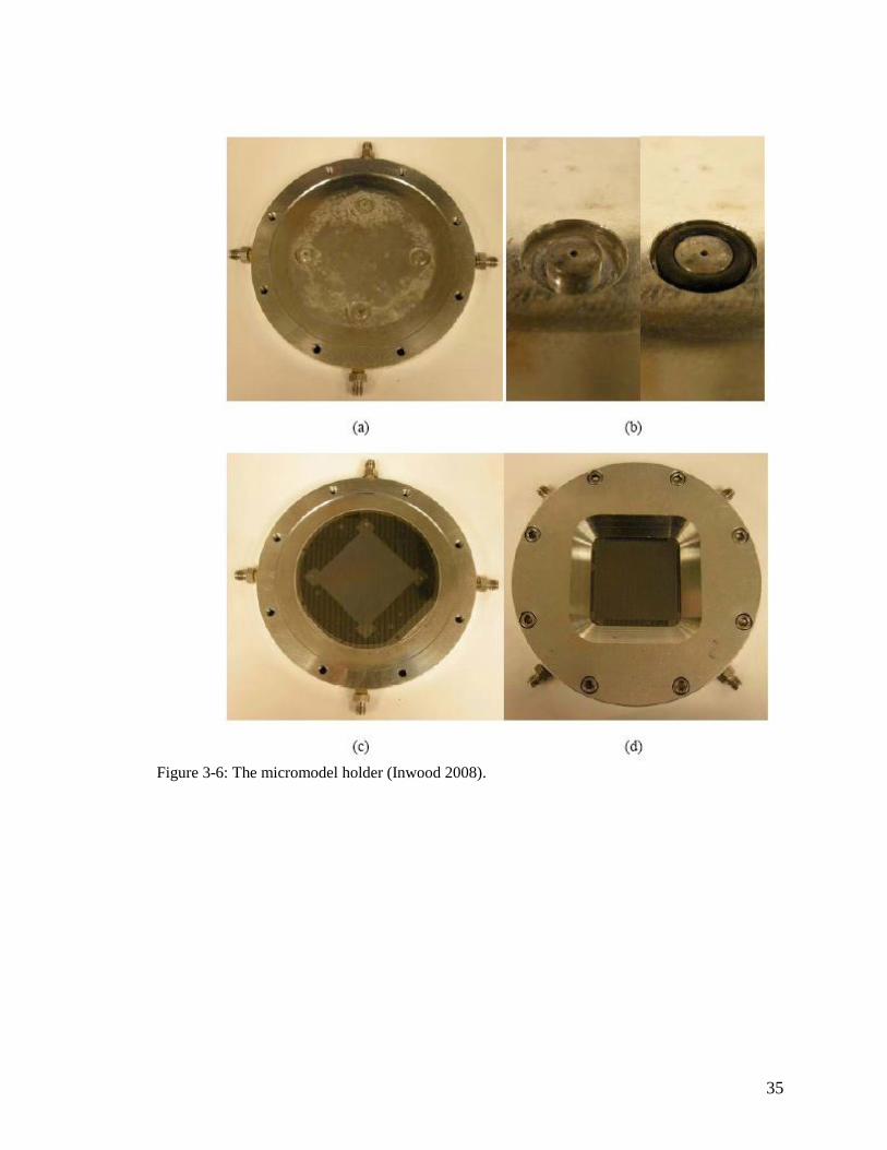
is a Nikon Coolpix P5100. The micromodel along with its holder is shown on Figure 3-6.
It has to be noted that the injected fluid has to go through the injection port and the o-ring
dead volume. Each port accounts for 0.1 ml in terms of volume which is more than twice
the micromodel pore volume (0.041 ml for Mask I micromodels and 0.047 ml for Mask II
micromodels). This eventually increases the uncertainty in volumetric analysis and thus
image analysis is the only technique used to quantify recovery.
3.3. Experimental Procedure
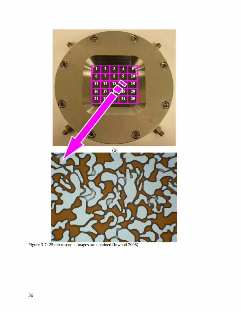
Several micromodel experiments were conducted. The microscopic images are collected
as shown on Figure 3-7. The micromodel area is divided into 25 squares. One image is
taken in each square with 100X and 200X magnification. In the results, a representative
image after each process is displayed.
In each micromodel experiment, CO2 is first injected to displace air if the micromodel is
new. After that, distilled water is injected, then brine, then oil to obtain initial oil
saturation. If the micromodel is used, it is cleaned with toluene to dissolve/remove
residing fluids. Iso-propanol is then injected to push the toluene out followed by distilled
water, brine, and then oil. Injection rates for a water flood or a surfactant flood was held
at a constant rate to achieve a Darcy velocity of 1 m/day. Before stating the experiment
procedures, the image analysis method has to be described.
3.3.1. Image Analysis
Matlab image analysis tools were utilized to quantify the remaining oil after each
flooding stage in the experiment. The code, shown on Appendix A.B, was initially
constructed by Buchgraber (2008) and then modified to enhance its speed. The main
principle of the code is to convert the Red Green Blue (RGB) image to a binary image
(black and white). The RGB cutoff values for oil is determined and then inputted into the
code. The code replaces pixels’ values above the cutoffs to one (white) and below the
26
cutoffs to zero (black). The number of zeros indicates how much “black” is in the image.
It has to be noted that the grain edges and sometimes parts of the etched surface of the
micromodel have the same RGB values as the oil. Hence, blackness due to the edge
effect (and etched surface) has to be subtracted from the “black” number. The edge effect
is determined by running the image analysis on a waterflooded micromodel. The average
“black” number in this case is used as the edge effect. For mask 1 micromodels, the edge
effect is about 32.6±4% while it is about 17.7±3% for mask 2 micromodels. After
subtracting the edge effect, the new “black” number is divided by the porosity (𝜑) of the
micromodel to obtain oil saturation (𝑆𝑜) as the following:
𝑆𝑜 =𝐵𝑙𝑎𝑐𝑘 − 𝐸𝑑𝑔𝑒 𝐸𝑓𝑓𝑒𝑐𝑡
𝜑 (3-1)
Results from the various experiments are now discussed.
3.3.2. Experiment I
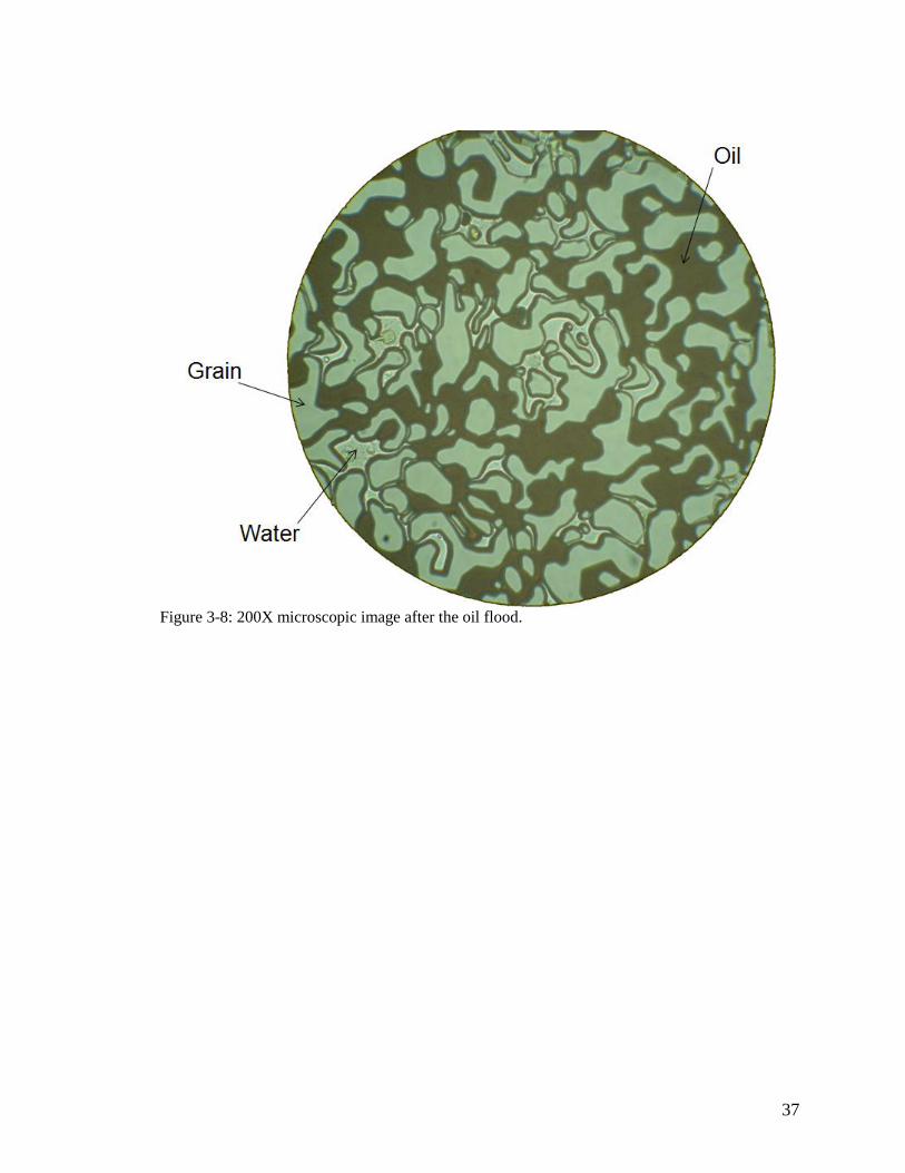
This is an early experiment where S-3A was injected in a secondary recovery mode. The
pore network is obtained from mask 1. Figure 3-8 shows a micromodel image after an oil
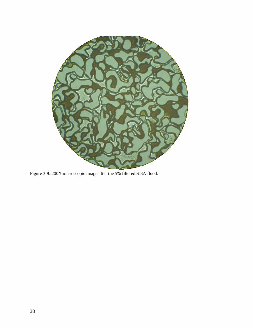
flood. Right after the oil flood, a 5% filtered S-3A solution with 0.2M Na2CO3 was
injected (Figure 3-9). The solution was filtered because it had a lot of suspended particles
that might cause blockage in the micromodel. Heating the sample did not dissolve these
particles. It can be seen in Figure 3-9 that some of the oil was not recovered (29%
remained) and that irreducible water occupied the small pores and throats of the
micromodel indicating that the model is water wet. Thus, 2% unfiltered S-3A was
injected and it did recover most of the oil where only 10% remained (Figure 3-10).
3.3.3. Experiment II
NEODOL 25-3 was used in a tertiary recovery mode. The pore network in this
micromodel is from mask 2. Figure 3-11 shows the microscopic image after an oil flood
(59% initial oil saturation). After that, about 1 pore volume brine was injected to recover
some of the oil as seen in Figure 3-12 (15% of oil remained). Then, 1% NEODOL 25-3
with 0.2 M Na2CO3 was injected. All the oil was recovered with the NEODOL as in
Figure 3-13 (5% of oil remained). However, a second phase was observed at this stage.
This phase is more likely to a surfactant or a microemulsion phase.
3.3.4. Experiment III
In this set of experiments, spontaneous imbibition is investigated. NEODOL 25-3 is
injected in a secondary mode at one end of a channel of the micromodel (injection port)
while keeping all the other ports open including the port at the other end of the injection
channel. NEODOL 25-3 flows through the channel and imbibes into the strongly water
wet micromodel. Spontaneous imbibition was performed for one day followed by a
forced imbibition for another day by closing the port at the other end of the channel. Two
27
experiments were conducted in this set: one held horizontally and the other held
vertically.
3.3.4.1.Horizontal Set-up
The purpose of this experiment is to have it as a frame of reference for the vertical
experiment. Image analysis indicates that the micromodel was 54% saturated with oil
after the oil flood (Figure 3-14). About 33% of oil remained after the spontaneous
imbibition (Figure 3-15). Forced imbibition recovered more oil and only 14% oil
remained in the micromodel (Figure 3-16).
3.3.4.2.Vertical Set-up
While all the previous experiments were conducted horizontally, the micromodel was
held vertically during surfactant injection in this experiment to include gravity effect at
low IFT values. Table 3-2 shows the Bond number calculations for this experiment. At 1
vol% of NEODOL 25-3, the pore size has to be at least about 900 microns to achieve a
Bond number of 10 as shown by Part A of the table. For an average pore size of 141
microns however, the Bond number is 0.25. Thus, an assumption was made that the pore
size (d) in the Bond number can be used as the oil drop vertical diameter. In the
horizontal experiment, the Bond number is about 0.015, using the etching depth of 35μm
as d, that shows that gravity effects are negligible in a horizontal set-up.
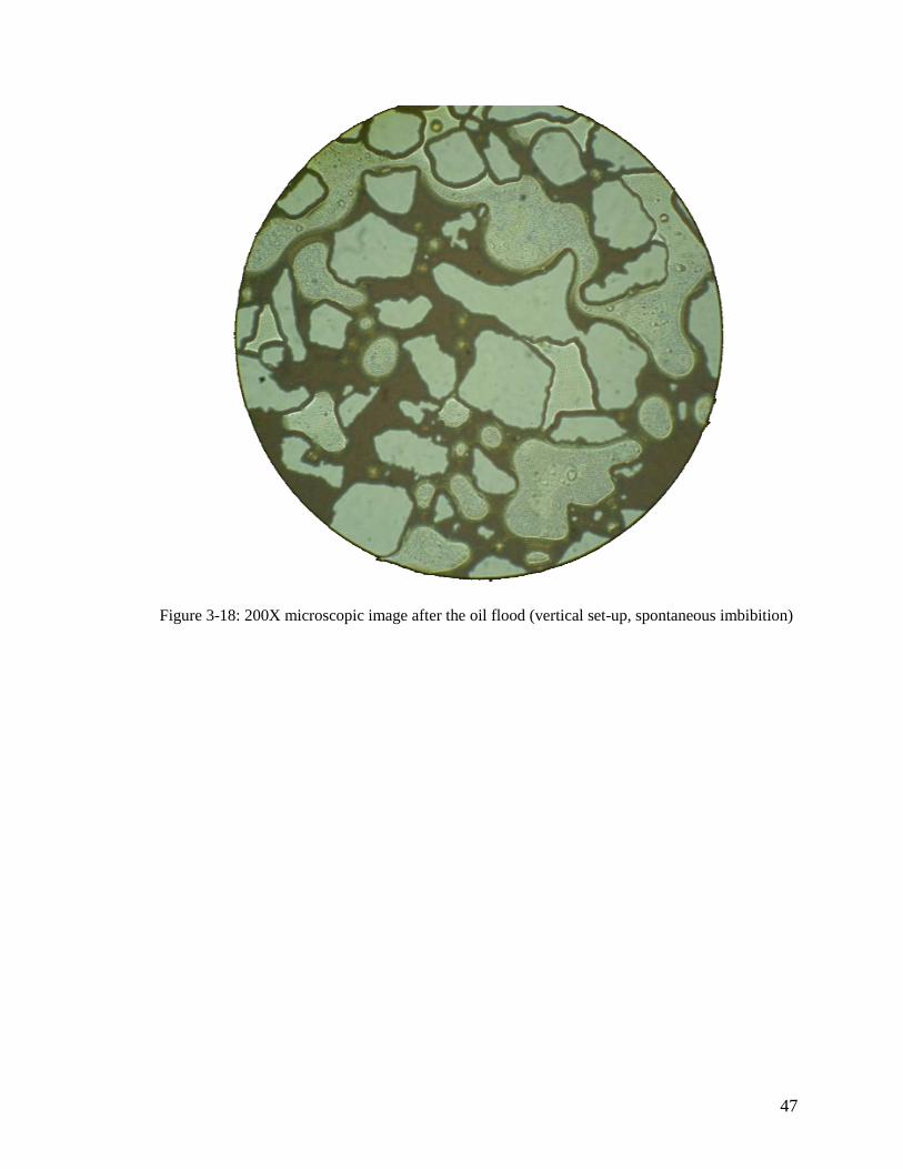
The experiment started with 54% of oil saturating the micromodel (Figure 3-17). The
spontaneous imbibition recovers some of the oil and 32% remained which is a 1%
marginal improvement compared to the horizontal set-up (Figure 3-18). The 1%
however, falls in the uncertainty range of the edge effect and a solid conclusion cannot be
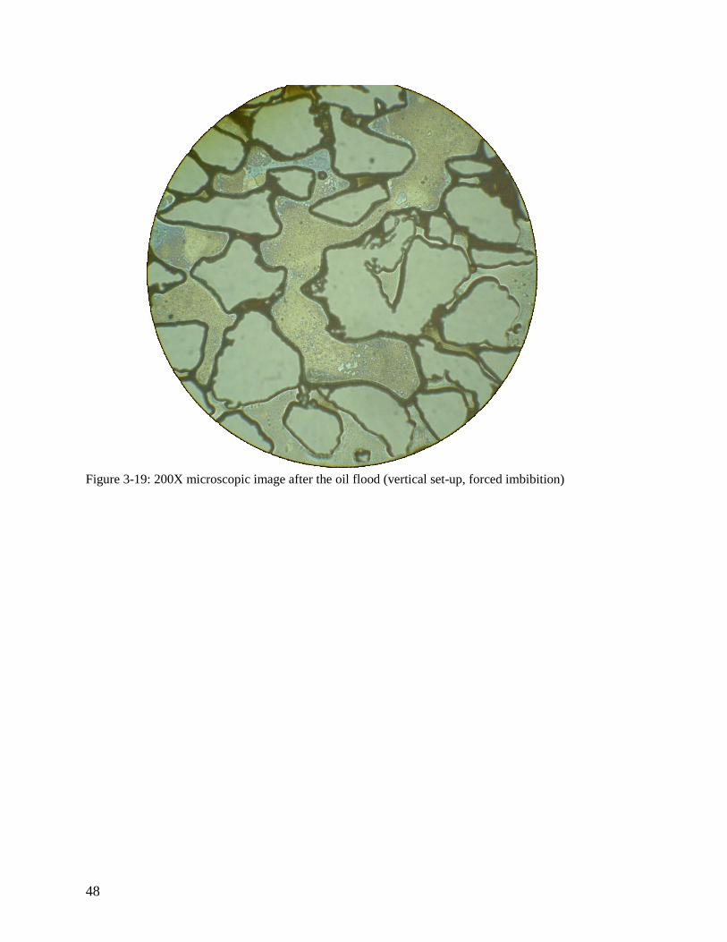
drawn from this number. The forced imbibition recovers most of the oil and only 6%
remains at the end of the experiment (Figure 3-19). This shows an 8% marginal
improvement over the horizontal set-up indicating that buyonce assisted in recovering
more oil. The remaining oil drops have very small diameters leading to very small Bond
numbers. Hence, gravity is not sufficient to displace the remaining oil out of the
micromodel.
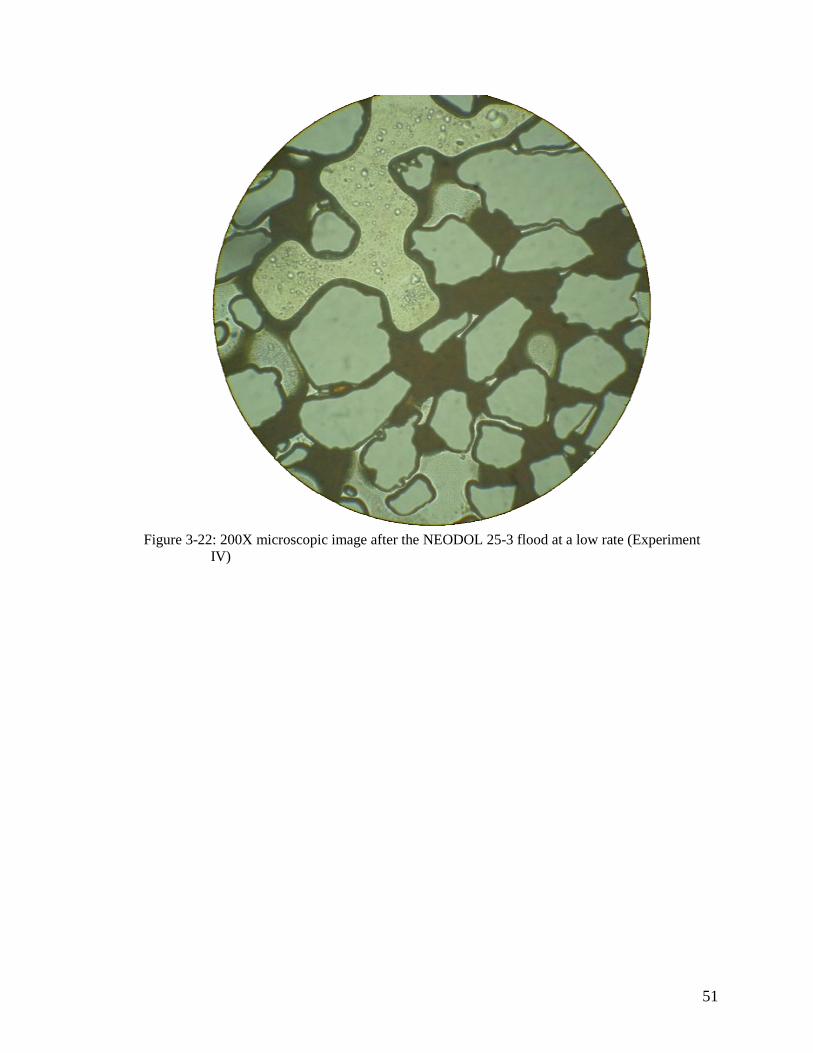
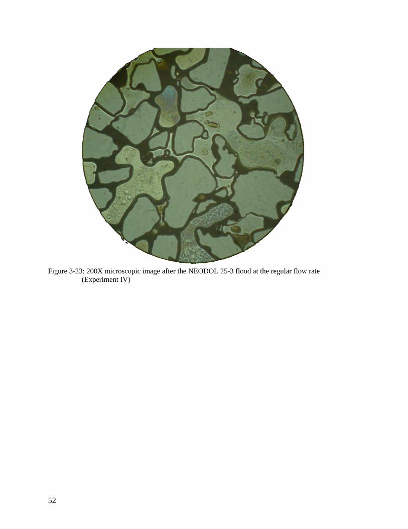
3.3.5. Experiment IV
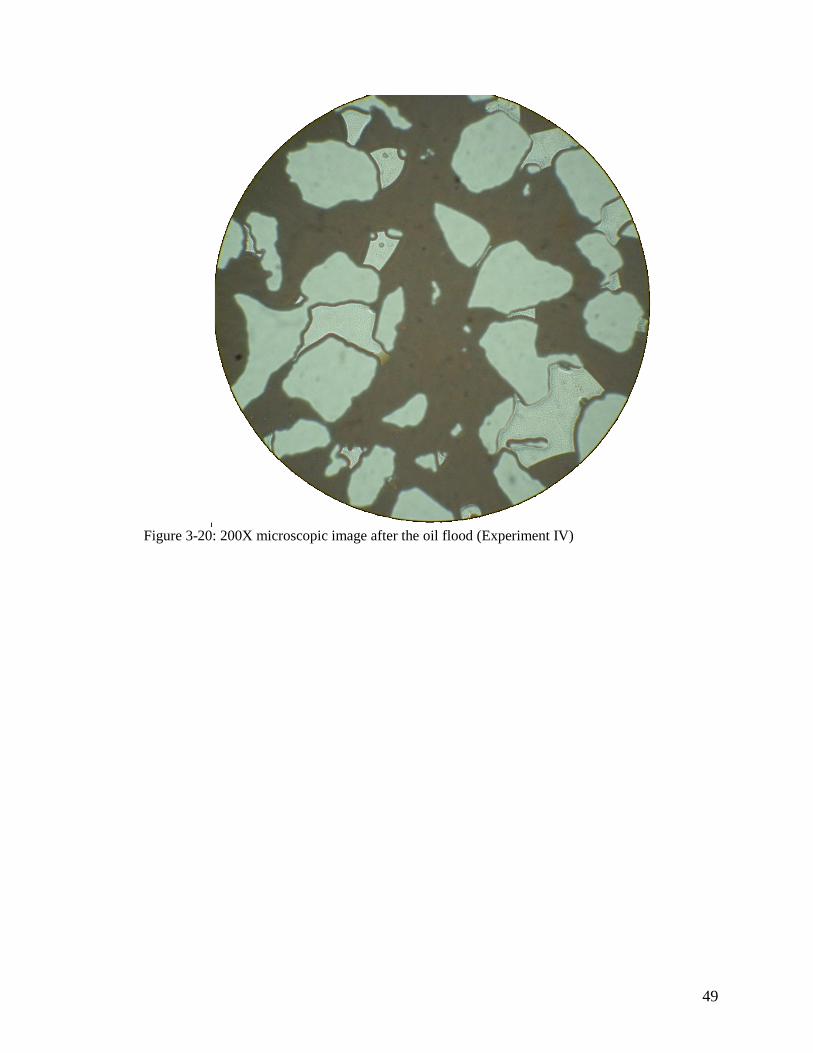
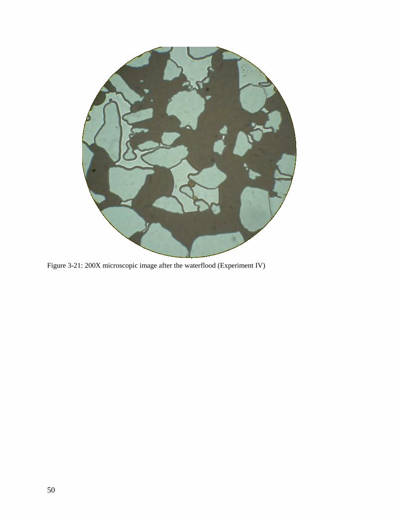
The purpose of this experiment is to mimic current conditions of waterflooded reservoirs.
In this experiment, the micromodel was waterflooded after an initial oil saturation of 48%
(Figure 3-20). Oil remaining after the waterflood is about 34% (Figure 3-21). A solution
of NEODOL 25-3 was injected at a tenth of the regular injection rate to replace the water
contacting the oil. The idea is to leave the surfactants contacting the oil to lower the IFT.
The micromodel is held vertically for four days and 24% of oil remained (Figure 3-22).
The injection rate was increased to the regular injection rate for 5 days and only 9% of
the oil remained (Figure 3-23). Bond numbers for the remaining oil drops are much
smaller than the cutoff and thus gravity effect is not strong enough to displace them.
28
Table 3-1: Permeability calculations of mask 2 micromodels.
viscosity (cp / Pa.s) 1 0.001 Length (cm / m) 5 0.05 Area (cm*micro m / m
2) 175 1.75E-06
P (psi) P (Pa) Q (ml/min) Q (m
3/s) k (m
2)
15 103421.35 0.94 1.57E-08 4.33E-12 20 137895.14 1.35 2.25E-08 4.66E-12 10 68947.57 0.56 9.33E-09 3.87E-12 4 27579.03 0.1 1.67E-09 1.73E-12 2 13789.51 0.01 1.67E-10 3.45E-13 15 103421.36 1 1.67E-08 4.60E-12
Average 3.26E-12 3.26 Darcy
29
Table 3-2: Bond number calculations for the vertical experiment.
A: Minimum pore size for 1% NEODOL 25-3
to achieve a Bond number of 10 B: Bond number for the average pore size
of 141 microns
Water density (g/cc) 1
Water density (g/cc) 1
Oil density (g/cc) 0.893
Oil density (g/cc) 0.893
gravity acceleration (m/s^2) 9.81
gravity acceleration (m/s^2) 9.81
pore size (m) 8.97E-04
pore size (m) 1.41E-04
IFT (N/m) 8.46E-05
IFT (N/m) 8.46E-05
Bond Number 10.00
Bond Number 0.25
30
Figure 3-1: Repeated square pattern in mask 1 (Inwood 2008).
31
Figure 3-2: Repeated pattern in mask 2.
0.64 cm
0.22 cm
32
Figure 3-3: Bonding apparatus (Hornbrook 1991).
Voltage Source (1200 V)
Cathode (grounded)
Glass Wafer
Etched Silicon
Wafer
Hot Plate (Anode;
Positively Charged)
+
-
33
Figure 3-4: A typical micromodel (Inwood 2008).
34
Figure 3-5: Schematic of apparatus.
35
Figure 3-6: The micromodel holder (Inwood 2008).
36
Figure 3-7: 25 microscopic images are obtained (Inwood 2008).
37
Figure 3-8: 200X microscopic image after the oil flood.
38
Figure 3-9: 200X microscopic image after the 5% filtered S-3A flood.
39
Figure 3-10: 200X microscopic image after the 2% unfiltered S-3A flood.
40
Figure 3-11: 200X microscopic image of the micromodel after the oil flood.
41
Figure 3-12: 200X microscopic image after the waterflood.
42
Figure 3-13: 200X microscopic image after the NEODOL 25-3 flood.
Brine phase
Surfactant/microemulsion
phase
43
Figure 3-14: 200X microscopic image after the oil flood (horizontal set-up).
44
Figure 3-15: 200X microscopic image after the NEODOL 25-3 flood (horizontal set-up,
spontaneous imbibition)
45
Figure 3-16: 200X microscopic image after the NEODOL 25-3 flood (horizontal set-up, forced
imbibition)
46
Figure 3-17: 200X microscopic image after the oil flood (vertical set-up)
47
Figure 3-18: 200X microscopic image after the oil flood (vertical set-up, spontaneous imbibition)
48
Figure 3-19: 200X microscopic image after the oil flood (vertical set-up, forced imbibition)
49
Figure 3-20: 200X microscopic image after the oil flood (Experiment IV)
50
Figure 3-21: 200X microscopic image after the waterflood (Experiment IV)
51
Figure 3-22: 200X microscopic image after the NEODOL 25-3 flood at a low rate (Experiment
IV)
52
Figure 3-23: 200X microscopic image after the NEODOL 25-3 flood at the regular flow rate
(Experiment IV)

53
54
Chapter 4
4. Discussion and Conclusion
This work consisted of two phases: a fluid characterization phase and a micromodel
experiment phase. The fluid characterization phase identified brine composition, the
appropriate surfactant to use, surfactant concentration, and sodium carbonate
concentration.
Hard water, containing calcium, is not recommended to be used when sodium carbonates
are used as alkaline. Precipitates, which might block pores/throats, form when sodium
carbonate was added to the brine. A decision was made to eliminate calcium chloride
from the brine composition. Another option is to add sodium metaborate as suggested by
Flaaten et al (2008) that prevents precipitations.
Dilute anionic surfactants with sodium carbonate reduce IFT to low values reducing
capillary forces that trap oil. Such reduction in IFT frees retained oil to the matrix and
eases its flow out of the micromodel. The surfactant screening indicates that NEODOL
25-3 is the most promising surfactant in terms of IFT reduction.
Thermal stability of surfactants was examined. This was performed by heating samples of
surfactant solutions for increasing intervals of time. Measurements of IFT are taken to see
if there is any significant change in the values that would indicate surfactant instability at
high temperatures. The study shows that the tested surfactants were thermally stable and
compatible for the given reservoir temperature (210˚F).
By conducting the micromodel experiments, it was visible that injection of dilute
surfactant solutions with sodium carbonate recovered most of the oil. This was concluded
by image analysis that shows that only 6-14% of oil remained after the surfactant flood
compared to 15-34% after a waterflood.
Bond number calculation indicates that for a 1 vol% NEODOL 25-3, the oil drop vertical
diameter has to be at least 900 μm for gravitational forces to become dominant. It was
shown that experiments conducted vertically lead to higher oil recovery than horizontal
experiments. This result was also enforced by the calculation of the Bond number for the
horizontal case. It was found to be 0.015 which is much less than the cutoff indicating a
negligible effect of gravity in a horizontal set-up. In other words, under similar
magnitudes of viscous and capillary forces, buoyancy is the additional recovery
mechanism in the vertical set up.
Spontaneous imbibition was achieved and significantly recovered retained oil. The
marginal improvement of remaining oil in the vertical set-up is 1% compared to the

55
horizontal set-up. This number however, is within the uncertainty range of the edge effect
and no solid conclusion can be drawn from this number.
For future work, it is recommended to include more surfactants in the study. The
screening criteria can also include wettability alteration and surfactant adsorption. A
possible next step is to vertically conduct core flooding experiments and use a CT
scanner to monitor front movements and saturation profiles. A 360˚ spontaneous
imbibition can be investigated by injecting the dilute surfactants in fractures that fully
surround the core.


57
Nomenclature
IFT: Interfacial tension
Bo: Bond number
Ca: Capillary number
d: Pore size diameter
f: angular velocity, msec/shaft rev
g: Gravity acceleration
krw: Water relative permeability
kro: Oil relative permeability
l: Liters
m: Meters
ml: Milliliters
M: Molar concentration
M: Mobility ratio
r: Elongated oil drop radius, meters
RGB: Red Green Blue
SNF: Stanford Nanofabrication Facility
So: Oil saturation
ui: Injectant Darcy velocity
WAG: Water-Alternating Gas
WOR: Water-Oil Ratio
μi: Injectant viscosity
μw: Water viscosity
μo: Oil viscosity
μm: Micrometers
ω: Spinning velocity
φ: porosity
ρ: Fluid density
σ: Interfacial tension
58
References
Aktas, F., Clemens, T., Castanier, L., & Kovscek, A. (2008). Viscous Oil
Displacement with Aqueous Associative Polymers. SPE 113264.
Adibhatla, B., Mohanty, K., K. (2006). Oil Recovery From Fractured Carbonates by
Surfactant-Aided Gravity Drainage: Laboratory Experiments and Mechanistic
Simulations. SPE 99773.
Buchgraber, M., Clemens, T., Castanier, L. M., & Kovscek, A. R. (2009). The
Displacement of Viscous Oil by Associative Polymer Solutions. SPE 122400.
Cinar, Y., Riaz, A., & Tchelepi, H. (2007). Experimental Study of CO2 Injection into
Saline Formations. SPE 110628.
Feng, Q., Di, L., Tang, G., Chen, Z., Wang, X., & Zou, J. (2004). A Visual Micro-
Model Study: The Mechanism of Water Alternative Gas Displacement in Porous
Media. SPE 89362 .
Flaaten, A., Nguyen, Q., Zhang, J., Mohammadi, H., & Pope, G. (2008). ASP
Chemical Flooding Without the Need for Soft Water. SPE 116754.
Gupta, R., & Mohanty, K. K. (2007). Temperature Effects on Surfactant-Aided
Imbibition Into Fractured Carbonates. SPE 110204.
Hamouda, A. A., & Gomari, K.A.R. (2006). Influence of Temperature on Wettability
Alteration of Carbonate Reservoir. SPE 99848.
Hirasaki, G., & Zhang, D. L. (2003). Surface Chemistry of Oil Recovery From
Fractured, Oil-Wet, Carbonate Formation. SPE 80988.
Hjelmeland, O. S., & Larronda, L. E. (1986). Experimental Investigation of the Effect
of Temperature, Pressure and Crude Oil Composition on Interfacial Properties.
SPE Reservoir Engineering 5(6) 321-328.
Hornbrook J., (1991). Visualization of Foam/Oil Interactions in a New, High
Resoltion Sandstone Replica Micromodel. Master thesis.
Inwood, S., (2008). High-Resolution Microvisual Study of High Mobility Ratio,
Immiscible Displacements. Energy Resources Engineering Department. Stanford
University. Master thesis.
Levitt, D. B., Jackson, A. C., Heinson, C., Britton, L. N., Malik, T., Dwarakanath, V.,
& Pope, G. A., (2006). Identification and Evaluation of High Performance EOR
Surfactants. SPE 100089.
Manning, C. D., & Scriven, L. E. (1977). On Interfacial Tension Measurement with a
Spinning Drop in Gyrostatic Equilibrium. Department of Chemical Engineering
and Materials Science. University of Minnesota.
Osterloh, W. T., & Jante, M. J. (1992). Surfactant-Polymer Flooding With Anionic
PO/EO Surfactant Microemulsions Containing Polyethylene Glycol Additives.
SPE/DOE 24151.
59
Rangel-German, E. R., & Kovscek, A. R. (2006). A Micromodel Investigation of
Two-Phase Matrix-Fracture Transfer Mechanisms. Water Resources Research.
Volume 42.
Schembre, J. M., Tang, G. Q., Kovscek, A. R. (2006). Interrelationship of
Temperature and Wettability on the Relative Permeability of Heavy Oil in
Diatomaceous Rocks. SPE Reservoir Evaluation and Engineering 239-250.
ShellChemicals. (2006). Product Data - Shell Chemicals. Retrieved 03 19, 2008, from
http://www.shellchemicals.com/neodol/1,1098,1470,00.html#130
Stanford Nanofabrication Facility. (2009). Equipment Summary. Retrieved 03 20,
2009, from https://spf.stanford.edu/SNF/equipment
STEPAN. (2006, 10 06). ONYXIDE 200. Retrieved 10 25, 2007, from
http://www.stepan.com/en/products/product_detail.asp?id=395
Tripathi, I., & Mohanty, K. K. (2007). Flow Instability Associated With Wettability
Alteration. SPE 110202.
Wang, A. A., & Gupta, A. (1995). Investigation of the Effect of Temperature and
Pressure on Wettability Using Modified Pendent Drop Method. SPE 30544.
Wellington, S. L., & Richardson, E. A. (1997). Low Surfactant Concentration
Enhanced Waterflooding. SPE 30748 .

61
Appendix A
A. Wafer Run Procedure
RUNNING PROCEDURES FOR
MICROMODEL FABRICATION
QING CHEN
SUPRI-A, STANFORD PETROLEUM
DEPARTMENT
FIRST WORK ON 8/2/04
VERSION 1.1, LAST UPDATED 10/26/06
REVISED BY: AMAR J ALSHEHRI AND
BOLIVIA VEGA ON JUNE 2008
4.1. General Description
Micromodel is a network of porous structures and channels, which is widely used for
experimental studies of 2-D fluid flow through porous media. Stanford Micromodel is
designed and fabricated by anodically bonding a Si wafer with etched pattern to a
transparent glass plate, providing optical access for flow visualization. This document
describes in details the micromodel fabrication procedures developed at Stanford
Petroleum Department over the past 30 years.
4.2. Process Overview
Materials:
4” Si wafer, K Prime, 4P <100> B S42565 (WaferNet, Inc.)
Borofloat 4” diameter X 0.043” thick, standard transparent finish 80/50 – 60/40
scratch/dig, flat to 3-4 waves/inch
The processes to fabricate Stanford Micromodel in order are:
Wafer precleaning
Photolithography
◦ Coating
◦ Exposing
◦ Developing
Deep etching
Resist removing and cleaning
Anodic bonding
Dicing (if necessary)
62
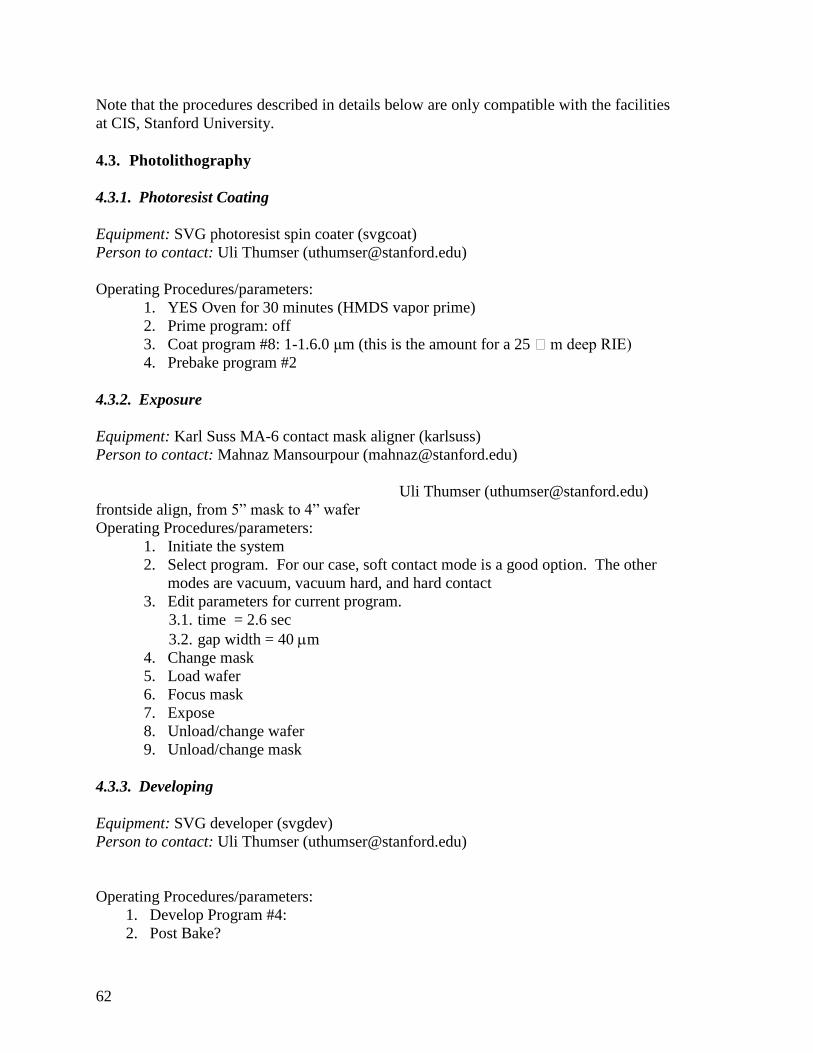
Note that the procedures described in details below are only compatible with the facilities
at CIS, Stanford University.
4.3. Photolithography
4.3.1. Photoresist Coating
Equipment: SVG photoresist spin coater (svgcoat)
Person to contact: Uli Thumser ([email protected])
Operating Procedures/parameters:
1. YES Oven for 30 minutes (HMDS vapor prime)
2. Prime program: off
3. Coat program #8: 1-1.6.0 μm (this is the amount for a 25 m deep RIE)
4. Prebake program #2
4.3.2. Exposure
Equipment: Karl Suss MA-6 contact mask aligner (karlsuss)
Person to contact: Mahnaz Mansourpour ([email protected])
Uli Thumser ([email protected])
frontside align, from 5” mask to 4” wafer
Operating Procedures/parameters:
1. Initiate the system
2. Select program. For our case, soft contact mode is a good option. The other
modes are vacuum, vacuum hard, and hard contact
3. Edit parameters for current program.
3.1. time = 2.6 sec
3.2. gap width = 40 m
4. Change mask
5. Load wafer
6. Focus mask
7. Expose
8. Unload/change wafer
9. Unload/change mask
4.3.3. Developing
Equipment: SVG developer (svgdev)
Person to contact: Uli Thumser ([email protected])
Operating Procedures/parameters:
1. Develop Program #4:
2. Post Bake?

63
3. Oven bake #2
4.4. Deep Etching
Equipment: STS multiplex ICP Deep Reactive Ion etcher (stsetch)
Person to contact: Nancy Latta ([email protected])
Operating Proceures/Parameters
Etch recipe: DEEP
Select a desired recipe and set it as current by clicking recipe field
Pre check: 400 Hz.
o During process: P about 10 Q about 3 and not fluctuating wildly.
Check and modify settings of the current recipe. Press RECIPE button in the
window of Press control–ICP. In the popped-out recipe window, check the
settings with the parameters from the STSetch logbook. For those standard
recipes, like DEEP, the only parameter that can be changed is the etching time.
With assumption that etching rate is constant, the desired etching time can be
easily determined from the desired etching depth. Remember to save recipe
before exiting the recipe menu if any setting is changed.
Unload wafer if necessary.
Load new wafer
Start etching process by pressing PROCESS button
Read parameters of machine conditions and write them down on the logbook.
Those parameters include
◦ He pressure and flow which can be read from the low small window on the
left side of the machine
◦ Chamber pressure (passivation and etch) which can be read from the right
lower part of the machine view window.
Unload wafer when etching is done.
4.5. Post-check
Check etching depth:
4.5.1. Using a microscope:
The depth between white and color is measured as the etching depth – photoresist
thickness (about 2 μm) (contact Nancy Latta for help)
4.5.2. Using Tencor P2 Profilometer:
The P2 has a stylus that physically touches the etched and the non-etched surface and
calculates the difference (contact Uli Thumser for help).
4.5.3. Using Zygo 3D Surface Profiler:
64
The Zygo relies on the reflectivity of different elevated surfaces (contact Uli Thumser for
help).
4.6. Resist Removal and Cleaning
Equipment: Nonmetal Wet Bench (wbnonmetal)
Person to contact: Uli Thumser ([email protected])
Matrix (O2 asher), wbnonmetal (sulfuric acid)
4.7. Anodic Bonding
Equipment: Power supply, Thermolyne hotplate, and Wet chemical cleaning stations
Operation Procedure:
Clean the materials that will be bonded. The standard clean is as follows:
Silicon wafers: 20 min Sulfuric/Peroxide Piranha (9:1 H2SO4:H2O2) clean at
120 oC, followed by 6-cycle deionized water rinse and spinning dry. This
cleaning process can be done with wbsilicide (gold-contaminated bath) at SNF
Lab.
Glass wafers: cleaned in Sulfuric/Peroxide Piranha (9:1 H2SO4:H2O2) for
about 10 minutes, rinsed by deionized water thoroughly, and then air dried.
This cleaning process can be done with wbsilicide (gold-contaminated bath) at
SNF Lab.
Anodic bonding
Place a cleaned wafer on a hotplate preheated to 350oC, with its etched side
facing up. The wafer is left on the plate for around 45 minutes, by which a
very thin SiO2 film is formed on the wafer surface and the wafer, initially
non-wetting, becomes water wetting.
Reduce the hotplate temperature down to 300oC and wait for the temperature
to be stabilized. Inspect the wafer surface for any dust that might deposit
during preheating period. Blow off any visible dust from the surface with
compressed clean air if necessary.
Place a cleaned glass wafer right on the top of the wafer, and align as desired.
Allow the wafers to heat for at least 1 minute.
Preset the voltage of the power supply between 900 and 1200 volts. Turn the
power supply to standby mode, and allow it to warm up for 2 minutes. The
anode of the power supply is connected to the hotplate and the other electrode
(cathode) is connected to an aluminum plate wrapped by a copper mesh.
Place the aluminum plate on the top of the glass wafer gently and then turn on
the power supply to apply a high voltage.
After 50 minutes, bonding should be achieved.

65
Turn off the electricity, remove the new micromodel from the hotplate using
tweeze, and allow it to cool to room temperature. Don’t leave the micromodel
on the hotplate for cooling. There are two reasons for not doing that: it takes
longer to cool the model; it was occasionally found that the glass got cracked
during cooling on the hotplate.

66
B. Image Analysis Code
function average=oilperc(dirname)
% Initilize white and black values
sumwhite=0;
sumblack=0;
% Obtain images
cd(dirname)
names=dir('*.JPG');
nnames=length(names);
oil=zeros(nnames,1);
% Define crop dimensions
i1=1000; j1=300;
width=1800; height=2050;
pixels = width * height / 100;
% Define RGB cutoffs for oil
R=110; G=115; B=90;
for i=1:nnames
fname=names(i).name
X =imread(fname);
X=imcrop(X,[i1 j1 width height]);
Y = (X(:,:,1)>R) + (X(:,:,2)>G) + (X(:,:,3)>B);
Y = floor(Y./3);
datei=['blackwhite' fname ];
imwrite(Y,datei,'jpg');
white=sum(sum(Y))/pixels
black=100-white
sumblack=sumblack+black;
sumwhite=sumwhite+white;
oil(i)=black;
black=0;
white=0;
end
averagewhite = sumwhite/nnames
averageblack = sumblack/nnames
oil
average = [averagewhite, averageblack]