J. Math. Anal. Appl. 410 (2014) 101–116

Contents lists available at ScienceDirect

Journal of Mathematical Analysis andApplications

www.elsevier.com/locate/jmaa

Lower previsions induced by filter maps

Gert de Cooman a, Enrique Miranda b,∗a Ghent University, SYSTeMS, Technologiepark, Zwijnaarde 914, 9052 Zwijnaarde, Belgiumb University of Oviedo, Dep. of Statistics and Operations Research, C-Calvo Sotelo s/n, 33007 Oviedo, Spain

a r t i c l e i n f o a b s t r a c t

Article history:Received 22 October 2012Available online 9 August 2013Submitted by V. Pozdnyakov

Keywords:Coherent lower previsionsn-Monotone capacitiesMinitive measuresFiltersChoquet integral

We investigate under which conditions a transformation of an imprecise probability modelof a certain type (coherent lower previsions, n-monotone capacities, minitive measures)produces a model of the same type. We give a number of necessary and sufficientconditions, and study in detail a particular class of such transformations, called filter maps.These maps include as particular models multi-valued mappings as well as other modelsof interest within imprecise probability theory, and can be linked to filters of sets and{0,1}-valued lower probabilities.

© 2013 Elsevier Inc. All rights reserved.

1. Introduction

In many practical problems, it is not uncommon to encounter situations with vague or imprecise knowledge about theprobabilistic information of the variables involved; this could be due to deficiencies in the observational process or conflictsbetween the opinions of several experts, amongst other things. In such cases, it may be advisable to consider impreciseprobability models as a more robust alternative to the classical models based on probability measures. These models includeas particular cases sets of probability measures [14], coherent lower previsions [19], n-monotone capacities [1], and necessitymeasures [11].

All these models are mathematically related to each other: sets of probability measures and coherent lower previsionsare equivalent, and they include n-monotone capacities as special cases. Necessity measures are in particular n-monotonefor any natural number n.

Interestingly, a transformation of such models—under a permutation of the possibility space, or more generally, underanother map that connects two possibility spaces—need not preserve their character. To give an example, it is not uncom-mon that a transformation of a necessity measure goes beyond the framework of necessity measures, and produces only acoherent lower prevision (probability). In this paper, we investigate under which conditions a transformation of the possibil-ity space, or of the associated space of real-valued functions defined on it, preserves different consistency notions: avoidingsure loss, coherence, n-monotonicity or being minimum preserving.

We show that for the first two we must consider so-called coherence preserving transformations, which are closely relatedto (but at the same time more general than) coherent lower previsions. We investigate their properties in Sections 3 and 4.We show in Section 7 that as particular cases of coherence preserving mappings, we have the notion of probability inducedby a random variable, but also the Markov operators considered in [17]. For the last two conditions, we show in Sections 5and 6 that a conditional model preserves n-monotonicity in addition to coherence if and only if it is a ∧-homomorphism,

* Corresponding author.E-mail addresses: gert.decooman@UGent.be (G. de Cooman), mirandaenrique@uniovi.es (E. Miranda).

0022-247X/$ – see front matter © 2013 Elsevier Inc. All rights reserved.http://dx.doi.org/10.1016/j.jmaa.2013.08.006

102 G. de Cooman, E. Miranda / J. Math. Anal. Appl. 410 (2014) 101–116

i.e. minimum preserving. We characterise minimum preserving coherent lower previsions, and show that they are in aone-to-one correspondence with filters of subsets of the possibility space.

This leads us to the second part of the paper, where we study in detail a particular type of mappings, called filtermaps, which we introduce in Section 8. They are maps that assign to any element of an initial space a filter of subsetsof a final space. But they can also be interpreted as minimum preserving transformations. We show that they include asparticular cases the lower previsions induced by multi-valued mappings as well as lower oscillation models, and we studythe properties of the lower prevision that results from combining a filter map with a lower prevision on the initial space.

2. Preliminaries

2.1. Coherent lower previsions

We begin with a brief discussion of coherent lower previsions. We refer to [19] for more details and background, and forthe proofs of all results mentioned in this section.

Consider a possibility space X . A gamble f on X is any bounded real-valued map on X . This is for instance the casefor the indicator I A of a subset A of X , where I A(x) takes the value 1 when x ∈ A and 0 when x /∈ A.

The set of all gambles on X is denoted by G (X ). This is a linear space: it is closed under point-wise addition andmultiplication by real numbers. It is moreover a lattice, that is, closed under point-wise maxima ∨ and minima ∧. We willbe interested in some particular transformations between sets of gambles.

Definition 1. Given two spaces X and Y , a map r :G (X ) → G (Y ) is called a ∧-homomorphism when r( f1 ∧ f2) = r( f1)∧r( f2) for all f1, f2 ∈ G (X ).

A real-valued map defined on a set of gambles is called a lower prevision. It can be given a behavioural interpretation:the lower prevision of a gamble f is the supremum price μ such that the transaction f −μ is desirable for a given subject.This interpretation lies at the basis of the following definitions:

Definition 2. A lower prevision on a set of gambles K ⊆ G (X ) is a functional P :K → R. It is said to avoid sure loss whenfor every n ∈N0 and f1, . . . , fn ∈ K :

n∑i=1

P ( f i)� sup

[n∑

i=1

f i

],

where N0 denotes the set of natural numbers (with zero). It is called coherent if and only if for all numbers n,m ∈ N0 andf0, f1, . . . , fn ∈ K :

n∑i=1

P ( f i) − mP ( f0) � sup

[n∑

i=1

f i − mf0

].

One example of coherent lower previsions are the so-called vacuous ones. For any non-empty subset A of X , the vacuouslower prevision relative to A is defined on G (X ) as

P A( f ) := infx∈A

f (x) for all f ∈ G (X ).

A lower prevision P on the set G (X ) of all gambles turns out to be coherent if and only if:

C1. P ( f ) � inf f for all gambles f on X ;C2. P (λ f ) = λP ( f ) for all gambles f on X and all real λ � 0;C3. P ( f + g) � P ( f ) + P (g) for all gambles f and g on X .

On the other hand, a coherent lower prevision defined on indicators of events only is called a coherent lower probability.To simplify the notation, we will sometimes use the same symbol A to denote a set A and its indicator I A , so we will writeP (A) instead of P (I A). Of particular interest are the {0,1}-valued coherent lower probabilities, which are related to filtersof events:

Definition 3. Let P(X ) denote the power set of a space X . A subset F of P(X ) is called a (proper) filter when itsatisfies the following properties:

F1. ∅ /∈ F ;F2. if A, B ∈ F then A ∩ B ∈ F ;F3. if A ∈ F and A ⊆ B then B ∈ F .

G. de Cooman, E. Miranda / J. Math. Anal. Appl. 410 (2014) 101–116 103

A filter F is called fixed1 if there is a non-empty subset A of X such that B ∈ F if and only if A ⊆ B , and it is called freeotherwise.

If P is a coherent lower probability on P(X ) that takes only the values 0 and 1, then the class {A ⊆ X : P (A) = 1}forms a filter; and, conversely, for any filter F of P(X ), the lower probability P given by P (A) = 1 if A belongs to F ,and 0 otherwise, is coherent. We denote by F(X ) the set of all filters over the space X .

If a lower prevision P avoids sure loss, then we can ‘correct’ it into a coherent lower prevision. This is done by meansof the procedure of natural extension, whose main properties are summarised in the following theorem:

Theorem 1. ([19].) Let P be a lower prevision with domain K that avoids sure loss. Let E P be the lower prevision on the set G (X ) ofall gambles given by

E P ( f ) := sup

{μ ∈R: f − μ�

n∑j=1

λ j(

f j − P ( f j))

for some n ∈N, λ j > 0, f j ∈ K

}, (1)

where N is the set of natural numbers (without zero).

(i) E P is a coherent lower prevision.(ii) E P is the smallest coherent lower prevision that satisfies E P ( f )� P ( f ) for all f ∈ K .

(iii) P is coherent if and only if E P ( f ) = P ( f ) for all f ∈ K .

Another particular case of coherent lower previsions with domain G (X ) are the linear previsions:

Definition 4. A lower prevision P defined on the set G (X ) of all gambles is called a linear prevision when it satisfiesP ( f + g) = P ( f ) + P (g) for every pair of gambles f , g , and moreover P ( f ) � inf f for every gamble f .

A linear prevision coincides with the expectation functional associated with its restriction to (indicators of) events, whichis a finitely additive probability. Moreover, a lower prevision P defined on the set G (X ) of all gambles is coherent if andonly if

P ( f ) = min{

P ( f ): P ∈M(P )}, (2)

where

M(P ) := {P � P : P is a linear prevision}is the credal set associated with P . In other words, a coherent lower prevision P is always the lower envelope of the setM(P ) of all linear previsions that dominate it, and as such it can be seen as a lower expectation functional. Moreover,a lower prevision P with domain K avoids sure loss if and only if M(P ) = ∅, and in that case its natural extension E P canbe obtained by taking the lower envelope of M(P ):

E P ( f ) = min{

P ( f ): P ∈M(P )}, (3)

and M(P ) = M(E P ).In particular, the vacuous lower prevision relative to a set A is the lower envelope of the set of linear previsions P that

assign probability 1 to A:

P A( f ) = min{

P ( f ): P (A) = 1 and P linear prevision}, (4)

and M(P A) = {P linear prevision: P (A) = 1}.

2.2. n-Monotone lower previsions

A particular case of coherent lower previsions are those called n-monotone:

Definition 5. Let n ∈ N. A lower prevision defined on the set G (X ) of all gambles is n-monotone if for all p ∈ N, p � n, andall f , f1, . . . , f p in G (X ):

∑I⊆{1,...,p}

(−1)|I| P

(f ∧

∧i∈I

f i

)� 0,

where, as before, ∧ is used to denote the point-wise minimum.

1 Sometimes fixed filters are called principal or degenerate.

104 G. de Cooman, E. Miranda / J. Math. Anal. Appl. 410 (2014) 101–116

n-Monotone lower previsions have been studied in detail in [8,18], to which we refer for more details and background,and for the proofs of all results mentioned in this section.

When n � 2, an n-monotone lower prevision P is in particular coherent provided that P (0) = 0 and P (1) = 1, and itcorresponds to the Choquet integral with respect to its restriction to events, which is called an n-monotone lower probability.A lower prevision that is n-monotone for all natural n is called ∞-monotone or completely monotone. This is for instancethe case for the vacuous lower prevision P A considered above, and more generally for all minimum or infimum preservinglower previsions:

Definition 6. A lower prevision defined on the set G (X ) of all gambles is minitive when P ( f ∧ g) = P ( f ) ∧ P (g) for everypair of gambles f , g on X , and infimum preserving when P (

∧i∈I f i) = ∧

i∈I P ( f i) for any non-empty family { f i: i ∈ I}of gambles on X . Similarly, a lower probability on P(X ) is called minitive when P (A ∩ B) = min{P (A), P (B)} for allA, B ⊆ X , and a necessity measure when P (

⋂i∈I Ai) = infi∈I P (Ai) for any non-empty family {Ai: i ∈ I} of subsets of X .

Any linear prevision P on G (X ) is always completely monotone, but it need not be minitive.

2.3. Conditional lower previsions

We may also consider lower previsions in a conditional context. Within the framework of this paper, we consider twospaces X and Y , and call conditional lower prevision any functional P (·|Y ) defined on G (X × Y ) that to any gamble f onX × Y assigns a gamble P ( f |Y ) on Y , where the value that P ( f |Y ) assumes in y ∈ Y is denoted by P ( f |y) and calledthe conditional lower prevision of f given that Y = y.

Definition 7. A conditional lower prevision P (·|Y ) on G (X × Y ) is called separately coherent when it satisfies the followingconditions:

SC1. P ( f |y)� infx∈X f (x, y),SC2. P (λ f |y) = λP ( f |y),SC3. P ( f + g|y)� P ( f |y) + P (g|y),

for any gambles f , g ∈ G (X × Y ), all real λ� 0 and all y ∈ Y .

If P (·|Y ) is a separately coherent conditional lower prevision on G (X × Y ) and P is a coherent lower prevision onG (Y ), their marginal extension is the coherent lower prevision on G (X × Y ) given by P (P (·|Y )). It corresponds to thesmallest lower prevision on G (X × Y ) that is coherent with both P and P (·|Y ), in the sense considered in [19]. Marginalextension generalises the Law of Total Probability to lower previsions.

3. Coherence preserving transformations

In this section, we investigate how to transform a lower prevision on some set of gambles over a space Y into a lowerprevision on gambles defined on another space X while still keeping most of its properties.

Definition 8. Let T :G (X ) → G (Y ) be a transformation between two sets of gambles. It is called coherence preserving whenit satisfies the following properties:

T1. inf(T f ) � inf f for all f ∈ G (X );T2. T (λ f ) = λT f for all f ∈ G (X ) and all real λ� 0;T3. T ( f + g)� T f + T g for all f , g ∈ G (X ).

A coherence preserving transformation T automatically satisfies the following properties:

T4. if f � g then T f � T g for all f , g ∈ G (X );T5. T ( f + μ) = T f + μ for all f ∈ G (X ) and all real μ.

The interest of this type of transformations lies in the following result:

Proposition 2. Let T :G (X ) → G (Y ) be a transformation between two sets of gambles. Then the following statements are equiva-lent:

(i) T is coherence preserving;(ii) for every coherent lower prevision P on G (Y ), the composition P ◦ T is a coherent lower prevision on G (X ).

G. de Cooman, E. Miranda / J. Math. Anal. Appl. 410 (2014) 101–116 105

Moreover, if T is coherence preserving, and the lower prevision P on G (Y ) avoids sure loss, then the lower prevision P ◦ T on G (X )

avoids sure loss as well.

Proof. Let us begin the proof of the equivalence by showing that the first statement implies the second. It suffices to provethat P ◦ T satisfies conditions C1–C3.

C1. For any gamble f in G (X ), (P ◦ T )( f ) = P (T f ) � P (inf T f ) � P (inf f ) = inf f , where the first inequality followsfrom the coherence of P and the second from T1.

C2. Given f in G (X ) and λ � 0, P (T (λ f )) = P (λT f ) = λP (T f ), where the first equality follows from T2 and the secondfrom the coherence of P .

C3. Given f , g ∈ G (X ), P (T ( f + g)) � P (T f + T g) � P (T f )+ P (T g), where the first inequality follows from T3 and thesecond from the coherence of P .

Conversely, assume that the second statement holds, consider any y ∈ Y , and take the degenerate linear previsionP {y} , given by P {y}(g) := g(y) for all gambles g on Y . Then P {y} ◦ T is a coherent lower prevision by assumption, and(P {y} ◦ T )( f ) = (T f )(y). Let us use this to show that T satisfies T1–T3.

T1. Since P {y} ◦ T is a coherent lower prevision for all y ∈ Y , we infer from C1 that inf f � (P {y} ◦ T )( f ) = (T f )(y),whence indeed inf(T f )� inf f , for any gamble f on X .

T2. Since P {y} ◦ T is a coherent lower prevision for all y ∈ Y , we infer from C2 that (T (λ f ))(y) = (P {y} ◦ T )(λ f ) =λ(P {y} ◦ T )( f ) = λ(T f )(y), whence indeed T (λ f ) = λT f , for any gamble f on X and any real λ � 0.

T3. Since P {y} ◦ T is a coherent lower prevision for all y ∈ Y , we infer from C3 that (T ( f + g))(y) = (P {y} ◦ T )( f + g)�(P {y} ◦ T )( f ) + (P {y} ◦ T )(g) = (T f )(y) + (T g)(y), whence indeed T ( f + g) � T f + T g , for all gambles f and g on X .

To complete the proof, assume that T is coherence preserving and consider a lower prevision P on G (Y ) that avoidssure loss. Then there is a linear prevision P on G (Y ) such that P � P . As a consequence, P ◦ T � P ◦ T , and we have justproved that P ◦ T is a coherent lower prevision, which is therefore in particular dominated by some linear prevision. Thisimplies that P ◦ T is dominated by some linear prevision, and as a consequence it avoids sure loss. �

A transformation T takes any ‘vector’ f in the linear space G (X ) to a ‘vector’ T f in the linear space G (Y ), whose‘components’ are the real numbers (T f )(y), y ∈ Y . This also means that we can interpret T as a ‘vector map’ with as‘component maps’ the real functionals T y :G (X ) →R, y ∈ Y , defined by

T y( f ) := (T f )(y) = (P {y} ◦ T )(y) for all f ∈ G (X ). (5)

We infer at once from our argumentation in the proof of Proposition 2 that:

Proposition 3. A transformation T :G (X ) → G (Y ) is coherence preserving if and only if each of its component maps T y = P {y} ◦ T ,y ∈ Y , is a coherent lower prevision on G (X ).

In other words, a coherence preserving transformation T :G (X ) → G (Y ) can be seen as a family T y , y ∈ Y , of coherentlower previsions on G (X ).

We can use this simple idea to prove a number of basic properties for coherence preserving transformations. The firstone is an envelope result akin to the one mentioned for coherent lower previsions in Eq. (2):

Proposition 4. A transformation T :G (X ) → G (Y ) is coherence preserving if and only if it is the component-wise lower envelopeof a set of coherence preserving linear transformations.

Proof. ‘Only if’. Let T be a coherence preserving transformation. Then for every y ∈ Y the lower prevision T y defined byEq. (5) is coherent. As a consequence, it is the lower envelope of the set of linear previsions M(T y). Define now the set Hof transformations

H := {T : G (X ) → G (Y ): (∀y ∈ Y )T y ∈M(T y)

},

then obviously T is the component-wise lower envelope of H . From Proposition 3, any T ∈ H is a coherence preservingtransformation, because its associated component maps are linear previsions, and therefore in particular coherent lowerprevisions. To see that T is a linear transformation, note that for any f , g ∈ G (X ) and all y ∈ Y :

T ( f + g)(y) = T y( f + g) = T y f + T y g = (T f + T g)(y),

and therefore T ( f + g) = T f + T g .‘If’. That T is a component-wise lower envelope of coherence preserving linear transformations means that for every

y ∈ Y the lower prevision T y defined by Eq. (5) is a lower envelope of linear previsions, and is therefore a coherent lowerprevision. Now use Proposition 3. �

Next, we show that a number of combinations of coherence preserving transformations produce another coherence-preserving transformation.

106 G. de Cooman, E. Miranda / J. Math. Anal. Appl. 410 (2014) 101–116

Proposition 5.

(i) Let {T i: i ∈ I} be a family of coherence preserving transformations, and let T := infi∈I T i be their component-wise lower envelope.Then T is coherence preserving.

(ii) Let T n be a sequence of coherence preserving transformations that converges point-wise towards some T :G (X ) → G (Y ). ThenT is coherence preserving.

(iii) Let T 1 and T 2 be coherence preserving transformations and let α ∈ (0,1). Then T := αT 1 + (1 − α)T 2 is coherence preserving.

Proof. Taking into account Proposition 3, it suffices to establish the corresponding properties for the coherent componentmaps. These have been proved in [19, Theorems 2.6.3–2.6.5]. �

In a similar vein, and taking into account the characterisation of coherence preserving functionals in Proposition 3, wecan extend most of the properties established for coherent lower previsions in [19, Section 2] to coherence preservingfunctionals.

4. Coherence preserving transformations and conditional lower previsions

Consider a coherence preserving transformation T :G (X ) → G (Y ). We have seen in Proposition 3 that its componentmaps T y are coherent lower previsions, and it follows from the discussion in Section 2.3 that if we let

P (h|y) = P(h(·, y)|y

) := T y(h(·, y)

) = (T h(·, y)

)(y) for all y ∈ Y and h ∈ G (X × Y ), (6)

then P (·|Y ) is a conditional lower prevision on G (X × Y ) that is separately coherent. Conversely, with a separately coher-ent conditional lower prevision P (·|Y ) on G (X × Y ), we can associate a transformation T defined by

(T f )(y) := P ( f |y) for all y ∈ Y and f ∈ G (X ) (7)

that is coherence preserving. In other words, Proposition 3 can be reformulated to state that there is a one-to-one corre-spondence between coherence preserving transformations and separately coherent conditional lower previsions, expressedby Eqs. (6) and (7).

Interestingly, if we have a coherent lower prevision P on G (Y ), and a coherence preserving transformation T :G (X ) →G (Y ) with associated conditional lower prevision P (·|Y ) via Eq. (6), then the transformed coherent lower prevision P ◦ T =P (P (·|Y )) is the marginal extension of P and P (·|Y ), as discussed in Section 2.3.

This correspondence points towards an interesting way of extending a transformation T :G (X ) → G (Y ) to a transfor-mation T̃ :G (X × Y ) → G (Y ), defined by

(T̃ h)(y) := (T h(·, y)

)(y) for all y ∈ Y and h ∈ G (X × Y ). (8)

This simple idea will turn out to be of crucial importance for the discussion further on.

5. ∧-Homomorphisms

Before we turn to the study of n-monotonicity, let us take a look at the transformations that preserve minitivity.

Proposition 6. Let T :G (X ) → G (Y ) be a transformation between two sets of gambles. Then the following statements are equiva-lent:

(i) T is a ∧-homomorphism;(ii) for every minitive lower prevision P on G (Y ), the composition P ◦ T is a minitive lower prevision on G (X ).

Proof. Let us begin the proof of the equivalence by showing that the first statement implies the second. Given f , g ∈ G (X )

and a minitive P , we have indeed that P (T ( f ∧ g)) = P (T f ∧ T g) = P (T f ) ∧ P (T g), so P ◦ T is minitive too.Conversely, assume that the second statement holds, consider any y ∈ Y , and consider the degenerate linear prevision

P {y} , given by P {y}(g) := g(y) for all gambles g on Y . It is clearly minitive, and therefore its component map T y = P {y} ◦ Tis minitive by assumption. Hence T ( f ∧ g)(y) = T y( f ∧ g) = T y f ∧ T y g , and therefore T ( f ∧ g) = T f ∧ T g for all gamblesf and g on G (X ), so T is a ∧-homomorphism. �

The argumentation in this proof leads at once to the following proposition:

Proposition 7. A transformation T :G (X ) → G (Y ) is a ∧-homomorphism if and only if each of its component maps T y = P {y} ◦ T ,y ∈ Y , is a minitive lower prevision on G (X ).

G. de Cooman, E. Miranda / J. Math. Anal. Appl. 410 (2014) 101–116 107

Because minitive lower previsions are completely monotone, they are also coherent if and only if they satisfy P (0) = 0and P (1) = 1. The following result provides a further characterisation.

Theorem 8. Let P be a coherent lower prevision on G (X ). Then the following statements are equivalent:

(i) P is minitive;(ii) the restriction of P to events is a {0,1}-valued lower probability;

(iii) there is a filter F := {A ⊆ X : P (A) = 1} such that P ( f ) = supF∈F infx∈F f (x) for all gambles f on X .

Proof. We begin by showing that the first statement implies the second. Assume that P is a minitive coherent lowerprevision. Then it follows that its restriction to events is a minitive lower probability. Assume ex absurdo that there is someevent A such that P (A) ∈ (0,1). Consider the gambles f := 1 and g := 2

P (A)I A . Then P ( f ) = 1 and P (g) = 2

P (A)P (A) = 2, so

P ( f ) ∧ P (g) = 1. On the other hand, f ∧ g = I A , so P ( f ∧ g) = P (A) < 1. This contradicts that P is minitive.To show that the second statement implies the third, assume that the restriction Q of P to events is a {0,1}-valued

lower probability on P(X ), which is coherent as a restriction of the coherent lower prevision P . It then follows from thediscussion in [19, Sections 2.9.8 and 3.2.6] that the set F := {A ⊆ X : P (A) = 1} is a (proper) filter, and that Q has aunique coherent extension to G (X )—which must therefore coincide with P —given by:

P ( f ) = supF∈F

infx∈F

f (x) for all gambles f on X . (9)

Finally, to show that the third statement implies the first, we must prove that the lower prevision P defined byEq. (9) is minitive. Consider any two gambles f and g on X . Then for any ε > 0 there are two events F1 and F2in F such that P ( f ) � infx∈F1 f (x) + ε and P (g) � infx∈F2 g(x) + ε, and therefore also P ( f ) � infx∈F1∩F2 f (x) + ε andP (g) � infx∈F1∩F2 g(x) + ε. Since F is a filter, we deduce that F1 ∩ F2 ∈ F and therefore

P ( f ∧ g) � infx∈F1∩F2

( f ∧ g)(x) = infx∈F1∩F2

f (x) ∧ infx∈F1∩F2

g(x) �(

P ( f ) − ε) ∧ (

P (g) − ε)�

(P ( f ) ∧ P (g)

) − ε.

We deduce that P ( f ∧ g) � P ( f )∧ P (g). The converse inequality follows from the monotonicity (due to coherence) of P . �We deduce from Theorem 8 that there is a one-to-one correspondence between filters of subsets of X and minitive

coherent lower previsions. If in addition we require that the lower prevision should be infimum preserving, we have thefollowing result:

Theorem 9. ([2, Section 8].) Let P be a coherent lower prevision on G (X ). Then P is infimum preserving if and only if its restrictionto events is a {0,1}-valued necessity measure.

Taking into account the discussion above, we deduce that an infimum preserving coherent lower prevision P is alsoassociated with a filter F of subsets of A ; but since P is infimum and not just minimum preserving, it follows that

P(⋂

F)

= infA∈F

P (A) = 1,

and as a consequence there is a smallest subset⋂

F of X with lower probability 1, so⋂

F ∈ F , meaning that F is fixed.This shows that infimum preserving coherent lower previsions are those associated with fixed filters, while more generallyminitive coherent lower previsions can also be associated with a free filter. It also shows that the only infimum preservingcoherent lower previsions are the vacuous lower previsions we have introduced in Section 2. Finally, when X is finite, theproperties of being infimum preserving and minimum preserving are equivalent, because in that case all filters are fixed;hence, in that case the vacuous lower previsions are the only minimum preserving ones.

6. n-Monotonicity preserving transformations

From transformations that preserve coherence, and transformations that preserve minitivity, we now turn to the studyof transformations that preserve n-monotonicity. We begin by showing that a coherence preserving transformation does notpreserve n-monotonicity in general:

Example 1. Let P be a coherent lower prevision on X that is not n-monotone. Consider the coherence preserving trans-formation T defined by (T f )(y) := P ( f ) for all f ∈ G (X ) and all y ∈ Y . Then for any n-monotone lower prevision Q onG (Y ), Q ◦ T coincides with P , which is not n-monotone.

The second type of transformations we have studied so far are the ∧-homomorphisms we have characterised in Section 5.It is not difficult to show that this type of transformations do preserve n-monotonicity:

108 G. de Cooman, E. Miranda / J. Math. Anal. Appl. 410 (2014) 101–116

Proposition 10. ([8, Lemma 6].) Let T :G (X ) → G (Y ) be a ∧-homomorphism and let P be a lower prevision on G (Y ). If P isn-monotone, then P ◦ T is n-monotone too.

Our next example shows that being a ∧-homomorphism, although sufficient, is not necessary for a coherence preservingtransformation to preserve n-monotonicity:

Example 2. Let P be an n-monotone lower prevision on X that is not minitive. Consider the coherence preserving trans-formation T defined by (T f )(y) := P ( f ) for all f ∈ G (X ) and all y ∈ Y . Then for any n-monotone lower prevision Q onG (Y ), Q ◦ T = P is n-monotone, so T preserves n-monotonicity, but it is not a ∧-homomorphism, because its componentmaps T y = P are not minitive; see Proposition 6.

Nevertheless, it is possible, with some modifications, to prove a characterisation of transformations that preserven-monotonicity as ∧-homomorphisms. For this we need to look at the extended transformations T̃ :G (X × Y ) → G (Y )

that can be used to turn a lower prevision P on G (Y ) into a lower prevision P ◦ T̃ on G (X × Y ), and that are given byEq. (8). We begin with some basic observations:

Proposition 11. Let T be a coherence preserving transformation between G (X ) and G (Y ).

(i) If P avoids sure loss, then so does P ◦ T̃ .(ii) If P is coherent, then so is P ◦ T̃ .

(iii) If P is n-monotone and T is a ∧-homomorphism, then P ◦ T̃ is n-monotone as well.(iv) If P is minitive and T is a ∧-homomorphism, then P ◦ T̃ is minitive as well.

Proof. If we consider that T̃ is a transformation between G (X × Y ) and G (Y ), we can consider its component maps T̃ y ,which are the lower previsions on G (X × Y ) given by:

T̃ y(h) = (T̃ h)(y) = (T h(·, y)

)(y) = T yh(·, y) for all gambles h on X × Y and all y ∈ Y .

This shows, taking into account Propositions 3 and 7, that T̃ is coherence preserving if T is, and that T̃ is a∧-homomorphism if T is. Now invoke Proposition 2 for the first two statements, Proposition 10 for the third, and Proposi-tion 6 for the fourth. �

We can show that a transformation T̃ preserves n-monotonicity if and only if T is a ∧-homomorphism:

Proposition 12. Let T :G (X ) → G (Y ) be a transformation between two sets of gambles. Then the following statements are equiva-lent:

(i) T is a ∧-homomorphism;(ii) for every n-monotone lower prevision P on G (Y ), the composition P ◦ T̃ is an n-monotone lower prevision on G (X × Y ).

Proof. The direct implication follows from Proposition 11.To prove the converse implication, assume that for every n-monotone lower prevision P on G (Y ), the composition P ◦ T̃

is an n-monotone lower prevision on G (X × Y ).We first prove that then T y must be monotone for every y ∈ Y . Assume ex absurdo that there are yo ∈ Y and gam-

bles f � g on X such that T yo f = T f (yo) > T g(yo) = T yo g . This means that with P := P {yo}—the completely monotone

vacuous lower prevision on G (Y ) relative to {yo}—the composition P ◦ T̃ is not completely monotone, because it is noteven monotone: if we define the gambles f̃ � g̃ on X × Y by letting f̃ (x, y) := f (x) and g̃(x, y) := g(x) for all x ∈ X andy ∈ Y , then T̃ y f̃ = (T f̃ (·, y))(y) = T f (y) = T y f and similarly T̃ y g̃ = T y g , which leads to the contradiction:

(P ◦ T̃ )( f̃ ) = T yo ( f ) > T yo (g) = (P ◦ T̃ )(g̃).

Next, assume ex absurdo that T is not a ∧-homomorphism, then there is, by Proposition 7, some y ∈ Y such that T y isnot minitive. Then there are gambles f1 and f2 on X such that T y( f1 ∧ f2) < T y f1 ∧ T y f2, since the monotonicity of T y

already implies that T y( f1 ∧ f2)� T y f1 ∧ T y f2.Consider any y′ = y, and the vacuous lower prevision P {y,y′} relative to {y, y′}, which is a completely monotone coherent

lower prevision on G (Y ). We only need to show that P {y,y′} ◦ T̃ is not 2-monotone. Consider any real number a in thenon-empty interval (T y( f1 ∧ f2), T y f1) and any real number b in the non-empty interval (T y( f1 ∧ f2), T y f2), and definethe gambles f , g on X × Y by:

f := aI{y′} + f1 I{y} and g := bI{y′} + f2 I{y}.

G. de Cooman, E. Miranda / J. Math. Anal. Appl. 410 (2014) 101–116 109

Then

T̃ f (z) = T f (·, z) =⎧⎨⎩

T y f1, z = y,

a, z = y′,0, elsewhere

and T̃ g(z) = T g(·, z) =⎧⎨⎩

T y f2, z = y,

b, z = y′,0, elsewhere,

and similarly

T̃ ( f ∧ g)(z) =⎧⎨⎩

T y( f1 ∧ f2), z = y,

a ∧ b, z = y′,0, elsewhere

and T̃ ( f ∨ g)(z) =⎧⎨⎩

T y( f1 ∨ f2), z = y,

a ∨ b, z = y′,0, elsewhere,

so

(P {y,y′} ◦ T̃ )( f ) = min{a, T y f1} = a,

(P {y,y′} ◦ T̃ )(g) = min{b, T y f2} = b,

(P {y,y′} ◦ T̃ )( f ∧ g) = min{

a ∧ b, T y( f1 ∧ f2)} = T y( f1 ∧ f2) < a ∧ b,

(P {y,y′} ◦ T̃ )( f ∨ g) = min{

a ∨ b, T y( f1 ∨ f2)} = a ∨ b,

taking into account that

a > T y( f1 ∧ f2), b > T y( f1 ∧ f2) ⇒ a ∧ b > T y( f1 ∧ f2) and

a < T y f1, b < T y f2 ⇒ a ∨ b < T y f1 ∨ T y f2 � T y( f1 ∨ f2).

As a consequence,

(P {y,y′} ◦ T̃ )( f ∨ g) + (P {y,y′} ◦ T̃ )( f ∧ g) < (a ∨ b) + (a ∧ b) = a + b = (P {y,y′} ◦ T̃ )( f ) + (P {y,y′} ◦ T̃ )(g),

and this implies that P {y,y′} ◦ T̃ is not 2-monotone. �We want to stress that, although the only T̃ that always preserve n-monotonicity are those for which T is a

∧-homomorphism, it does not hold that T preserves n-monotonicity if and only if it is a ∧-homomorphism, as we havealready seen in Example 2. This is because when T is a ∧-homomorphism between G (X ) and G (Y ) then T̃ is also a∧-homomorphism between G (X × Y ) and G (Y ), but the converse is not necessarily true.

7. Examples

In this section, we discuss a number of particular cases of coherence preserving transformations.

7.1. Liftings

Consider a map t :Y → X and its associated lifting T :G (X ) → G (Y ) given by T ( f ) := f ◦t for gambles f on X . ThenT is a coherence preserving transformation, which moreover satisfies T3 with equality, and given y ∈ Y , the componentmap T y of T , given by Eq. (5), is the degenerate linear prevision P {t(y)} .

In the special case that Y = X , the relationship between a coherent lower prevision P and its transformation P ◦ Tlies at the basis of the notions of weak and strong invariance discussed in [5]. Two particular cases are of interest: theshift transformations, leading to a treatment of time-invariance, where X = N and t(n) := n + 1 ([5, Section 8] and [19,Section 2.9.5]); and the permutations of a finite space X that give rise to a discussion of exchangeable lower previsions ([7]and [19, Section 9.5]).

The lower prevision induced by a lifting transformation can be seen as a generalisation to an imprecise-probabilistic con-text to the notion of probability induced by a map. In this sense, these notions also lead to the convergence in distributionresults for coherent lower previsions in [7, Theorem 6].

7.2. Transition operators

In a series of papers on the dynamics of Markov chains in an imprecise probability context [3,4,12], De Cooman etal. introduce and study lower transition operators T :G (X ) → G (X ), which are, essentially, coherence preserving trans-formations between the set G (X ) of all gambles on a finite state space X of a Markov chain and itself. These operatorsare the imprecise-probabilistic counterparts of transition matrices, and they allow for a complete characterisation of thedynamical behaviour of a Markov chain with imprecise transition probabilities. They are defined as follows: T f (x) := P ( f |x)

110 G. de Cooman, E. Miranda / J. Math. Anal. Appl. 410 (2014) 101–116

is the conditional lower prevision of a gamble f (Xn+1) on the state Xn+1 at time n + 1, when the Markov chain is in stateXn = x at time n.

We deduce from Section 4 that these transition operators can be seen as coherence preserving transformations, and fromSection 6 that they preserve n-monotonicity when they are minitive.

7.3. Markov operators

In [17], Škulj defines the following operators, which generalise conditional (linear) expectations:

Definition 9. (See [17, Definition 1].) Let H ,K be two linear subspaces of G (X ) that include all constant gambles. Alinear operator T :H → K that is monotone [ f � g ⇒ T ( f ) � T (g)] and such that T (1) = 1 is called a Markov operator.

Škulj discusses how to model risk and uncertainty aversion in a context of imprecision by means of a notion of invariancewith respect to a set of Markov operators. When H = K = G (X ), a Markov operator is a particular case of a coherencepreserving transformation: T2 and T3 hold because T is a linear operator. With respect to T1, note that for any gamblef ∈ G (X ), T ( f ) � T (inf f ) = inf f , where the inequality follows from the monotonicity of T and the equality from itslinearity and the fact that T (1) = 1.

7.4. Multi-valued maps

Let Γ :Y → P(X ) be a multi-valued map, and use it to define the transformation T :G (X ) → G (Y ) by T f (y) :=infx∈Γ (y) f (x). This transformation is coherence preserving, because its associated component maps T y are the vacuouslower previsions relative to the sets Γ (y), which are in particular coherent and infimum preserving: they are associatedwith the fixed filters determined by the sets Γ (y).

These types of coherence preserving transformations were investigated in detail in [16], and will be generalised bythe filter maps we will introduce in Section 8. We can identify T with a conditional lower prevision P (·|Y ), in such away that each P (·|y) is the vacuous lower prevision relative to Γ (y). Taking into account Proposition 11, we see thatthe composition of this coherence preserving transformation with a coherent lower prevision is again a coherent lowerprevision. In fact, since T is a ∧-homomorphism, the same result shows that this coherence preserving transformationpreserves n-monotonicity too.

This approach allows us to generalise some of the main concepts from random set theory to a context of imprecise-probabilistic information about the initial probability space Y . In Section 8, we will see that this generalisation can betaken one step further by means of filter maps.

8. Filter maps

When we combine the results of Propositions 7 and 12 with Theorem 8, we see that the transformations T that are guar-anteed to preserve n-monotonicity are exactly the ones whose component maps T y are minitive coherent lower previsions,meaning that there is some filter Φ(y) of subsets of X such that

T yh = supF∈Φ(y)

infx∈F

h(x, y) for all gambles h on X × Y .

In this section, we study these transformations in some detail. But we begin by providing yet another way of motivatingtheir study.

8.1. Motivation

Consider two variables X and Y assuming values in the non-empty (but not necessarily finite) sets X and Y .Let us first look at a single-valued map γ between the spaces Y and X . Given a linear prevision P on G (Y ), such

a map induces a precise probability Pγ on G (X ) by Pγ (A) := P (γ −1(A)) = P ({y ∈ Y : γ (y) ∈ A}) for all A ⊆ X , orequivalently

Pγ ( f ) := P ( f ◦ γ ) for all gambles f on X , (10)

which is a well-known ‘change of variables result’ for previsions (or expectations): If we have a variable Y , and the variableX is given by X := γ (Y ), then any gamble f (X) on the value of X can be translated back to a gamble f (γ (Y )) = ( f ◦γ )(Y )

on the value of Y , which explains where Eq. (10) comes from: if the uncertainty about Y is represented by the model P , thenthe uncertainty about X = γ (Y ) is represented by Pγ . This can also be seen as an application of the lifting procedure fromSection 7.1.

There is another way of motivating the same formula, which lends itself more readily to generalisation. We can interpretthe map γ as conditional information: if we know that Y = y, then we know that X = γ (y). This conditional information canbe represented by a so-called conditional linear prevision P (·|Y ) on G (X ), defined by

G. de Cooman, E. Miranda / J. Math. Anal. Appl. 410 (2014) 101–116 111

P ( f |y) := f(γ (y)

) = ( f ◦ γ )(y) for all gambles f on X . (11)

It states that conditional on Y = y, all probability mass for X is located in the single point γ (y). If P ( f |Y ) is the gambleon Y that assumes the value P ( f |y) in y, then clearly P ( f |Y ) = ( f ◦ γ )(Y ), which allows us to rewrite Eq. (10) as:

Pγ ( f ) = P(

P ( f |Y ))

for all gambles f on X , (12)

which shows that Eq. (10) is actually a special case of the Law of Iterated Expectations, the expectation form of the Law ofTotal Probability, in classical probability (see, for instance, [9, Theorem 4.7.1]).

Assume now that, more generally, the relation between X and Y is determined as follows. There is a so-called multi-valued map Γ :Y → P(X ) that associates with any y ∈ Y a non-empty subset Γ (y) of X , and if we know that Y = y,then all we know about X is that it can assume any value in Γ (y). There is no immediately obvious way of representing thisconditional information using a precise probability model. If we want to remain within the framework of precise probabilitytheory, we must abandon the simple and powerful device of interpreting the multi-valued map Γ as conditional informa-tion. But if we work with the theory of imprecise probabilities, as we are doing here, it is still perfectly possible to interpretΓ as conditional information that can be represented by a special conditional lower prevision P (·|Y ) on G (X ), where

P ( f |y) = PΓ (y)( f ) = infx∈Γ (y)

f (x) for all gambles f on X (13)

is the vacuous lower prevision relative to the event Γ (y); see Section 7.4 for more details. Given information about Y in theform of a coherent lower prevision P on G (Y ), it follows from Walley’s Marginal Extension Theorem (see [19, Section 6.7])that the corresponding information about X is the lower prevision PΓ on G (X ) defined by

PΓ ( f ) = P(

P ( f |Y ))

for all gambles f on X , (14)

which is an immediate generalisation of Eq. (12). This formula provides a well-justified method for using the conditionalinformation embodied in the multi-valued map Γ to turn the uncertainty model P about Y into an uncertainty model PΓ

about X . This approach has been introduced and explored in great detail by Miranda et al. [16].What we intend to do here, is take this idea of conditional information one useful step further. To motivate going

even further than multi-valued maps, assume that the information about the relation between X and Y is the following:If we know that Y = y, then all we know about X is that it lies arbitrarily close to γ (y), in the sense that X lies inside anyneighbourhood of γ (x). We are assuming that, in order to capture what ‘arbitrarily close’ means, we have provided X witha topology T of open sets. We can model this type of conditional information using the conditional lower prevision P (·|Y )

on G (X ), where

P ( f |y) = PNγ (y)( f ) = sup

N∈Nγ (y)

infx∈N

f (x) for all gambles f on X (15)

is the lower prevision associated with the neighbourhood filter Nγ (y) of γ (y). Information about Y in the form of acoherent lower prevision P on G (Y ) can now be turned into information P (P (·|Y )) about X , via this conditional model,using Eq. (14). This is the idea behind the notion of filter maps we define next.

8.2. Definition and main properties

So, given this motivation, let us try and capture these ideas in an abstract model.

Definition 10. A filter map Φ from Y to X , is a map Φ :Y → F(X ) that associates a proper2 filter Φ(y) with eachelement y of Y .

We can use filter maps to model some type of conditional information, which can be represented by a (specific) con-ditional lower prevision. In order to do this, given a filter map Φ , we associate with any gamble f on X × Y a lowerinverse f◦ (under Φ), which is the gamble on Y defined by

f◦(y) = PΦ(y)

(f (·, y)

) = supF∈Φ(y)

infx∈F

f (x, y) for all y in Y , (16)

where, of course, PΦ(y) is the lower prevision on G (X ) associated with the filter Φ(y) of X . Let us check that this lowerprevision is coherent:

Proposition 13. The lower prevision PΦ(y) on G (X ) associated with the filter Φ(y) of X is coherent.

2 Although in this paper we are only dealing with proper filters—i.e. we assume that ∅ /∈ Φ(y)—it is also possible to manage without this and similarassumptions, following the ideas in [16, Technical Remarks 1 and 2].

112 G. de Cooman, E. Miranda / J. Math. Anal. Appl. 410 (2014) 101–116

Proof. This is an immediate consequence of Theorem 8, taking into account the one-to-one correspondence between filtersand minitive coherent lower previsions. �

Similarly, we define for any gamble g on X its lower inverse g• (under Φ) as the gamble on Y defined by

g•(y) = PΦ(y)(g) = supF∈Φ(y)

infx∈F

g(x) for all y in Y . (17)

Eqs. (16) and (17) are obviously very closely related to, and inspired by, the expressions (11), (13) and (15). In particular,we find for any A ⊆ X × Y that (I A)◦ = I A◦ , where we let

A◦ = {y ∈ Y :

(∃F ∈ Φ(y))

F × {y} ⊆ A}

denote the so-called lower inverse of A (under Φ). And if B ⊆ X , then

(B × Y )◦ = B• = {y ∈ Y :

(∃F ∈ Φ(y))

F ⊆ B}

is the set of all y for which B occurs eventually with respect to the filter Φ(y).If we consider the transformation T :G (X ) → G (Y ) with component maps T y := PΦ(y) , then f◦ = T̃ f for any gamble

f on X × Y , and g• = T g for any gamble g on X . We know from the discussion in the previous sections that T and T̃preserve coherence and n-monotonicity.

Now consider any lower prevision P on Y that avoids sure loss. Then we can consider its natural extension E P , and useit together with the filter map Φ to construct an induced lower prevision P ◦ := E P ◦ T̃ on G (X × Y ):

P ◦( f ) = E P ( f◦) for all gambles f on X × Y . (18)

The so-called X -marginal P • := E P ◦ T of this lower prevision is the lower prevision on G (X ) given by

P •(g) = E P (g•) for all gambles g on X . (19)

Eqs. (18) and (19) are very closely related to, and inspired by, the expressions (10), (12), and (14). Induced lower previsionsare what results if we use the conditional information embodied in the filter map to turn an uncertainty model about Yinto an uncertainty model about X . This is because filter maps are in a one-to-one correspondence with minitive conditionallower previsions, taking into account the results in Sections 5 and 6.

We immediately deduce the following result:

Proposition 14. Let n ∈ N and let P be a lower prevision that avoids sure loss, and is defined on a subset of G (Y ). Let Φ be a filtermap from Y to X , and let P ◦ be the lower prevision given by Eq. (18). Then the following statements hold:

(i) P ◦ is a coherent lower prevision.(ii) If E P is n-monotone, then so is P ◦ .

Proof. Since E P is coherent, we infer from Proposition 11 that P ◦ = E P ◦ T̃ is coherent as well. The same result guaranteesthat if E P is n-monotone, then so is P ◦ , because T is a ∧-homomorphism by Proposition 7 and Theorem 8. �

As a particular case of the above results we have filter maps that associate with any y ∈ Y a fixed filter Φ(y) of subsetsof X . If we denote by Γ (y) the smallest subset in this filter, then we can define a multi-valued map Γ :Y → P(X ).The conditional lower prevision P (·|Y ) associated with this filter map is precisely the one considered in [16], that we havealready discussed in Section 7.4; many of the results we establish in this section constitute generalisations of results in [16]to arbitrary filter maps.

Remark 1. Another interesting particular case is that when Y = X and our filter map associates, with any y ∈ Y , the filterΦ(y) of all neighbourhoods of y under a certain topology in Y . Then the lower inverse defined in Eq. (17) produces

g•(y) = PΦ(y)(g) = supF∈Φ(y)

infz∈F

g(x) for all y in Y .

This is called a lower oscillation model in [6], and it can be seen to model the assessment that all the probability mass isconcentrated around y. This was the idea behind the motivation of filter maps we gave in Eq. (15).

Now, given a linear prevision π on the class of continuous gambles over a compact metric space, it can be proved thatits natural extension to all gambles is uniquely determined by its value on lower semi-continuous gambles, and that theseare precisely the lower oscillations defined in the above equation. This natural extension is moreover the lower envelope ofthe linear extensions of the linear prevision π to the class of gambles, and we can use the lower oscillations to characterisethose gambles for which there is a unique extension. See [6] for more details. �

G. de Cooman, E. Miranda / J. Math. Anal. Appl. 410 (2014) 101–116 113

8.3. Equivalent representations

Next, let us define a prevision kernel from Y to X as any map K from Y × G (X ) to R such that K (y, ·) is a linearprevision on G (X ) for all y in Y . Prevision kernels are clear generalisations of probability or Markov kernels [13, p. 20],but without the measurability conditions. They are in a one-to-one correspondence with separately coherent conditionallinear previsions. We can extend K (y, ·) to a linear prevision on G (X × Y ) by letting K (y, f ) = K (y, f (·, y)) for allgambles f on X × Y . For any lower prevision P on Y that avoids sure loss, we denote by P K the lower prevision onG (X × Y ) defined by

P K ( f ) = E P(

K (·, f ))

for all gambles f on X × Y .

Obviously, if P is a linear prevision on G (Y ), then P K is a linear prevision on G (X × Y ). As an immediate consequence,P K is always a coherent lower prevision on G (X × Y ), as a lower envelope of linear previsions (Eq. (2)). We also use thefollowing notation:

K(Φ) = {K : (∀y ∈ Y )K (y, ·) ∈ M(PΦ(y))

} = {K : (∀y ∈ Y )

(∀A ∈ Φ(y))

K (y, A) = 1}, (20)

where the last equality follows from Eq. (4). The set K(Φ) can be seen as the set of conditional linear previsions thatdominate the conditional lower prevision associated with the filter map Φ . The next proposition can be seen as a specialcase of Walley’s lower envelope theorem for marginal extension [19, Theorem 6.7.4]. Our proof closely follows Walley’soriginal proof.

Proposition 15. Let P be a lower prevision that avoids sure loss, and is defined on a subset of G (Y ). Let Φ be a filter map from Yto X , and let P ◦ be the lower prevision given by Eq. (18). Then for all K ∈ K(Φ) and P ∈ M(P ), P K ∈ M(P ◦); and for all gambles fon X × Y there are K ∈ K(Φ) and P ∈M(P ) such that P ◦( f ) = P K ( f ).

Proof. First, fix any P in M(P ) and any K ∈ K(Φ). Consider any gamble f on X × Y . We infer from Eqs. (16) and (20)that K (y, f ) � f◦(y) for all y ∈ Y , and therefore P K ( f ) = P (K (·, f )) � P ( f◦) � E P ( f◦) = P ◦( f ), where the first inequalityfollows from the coherence [monotonicity] of the linear prevision P , and the second from Eq. (3). This shows that P K ∈M(P ◦).

Next, fix any gamble f on G (X ×Y ). We infer from Eqs. (2) and (20) and the coherence of the lower previsions PΦ(y) ,y ∈ Y [Proposition 13] that there is some K ∈ K(Φ) such that f◦ = K (·, f ). Similarly, there is some P ∈ M(P ) such thatE P ( f◦) = P ( f◦), and therefore P ◦( f ) = P (K (·, f )) = P K ( f ). �

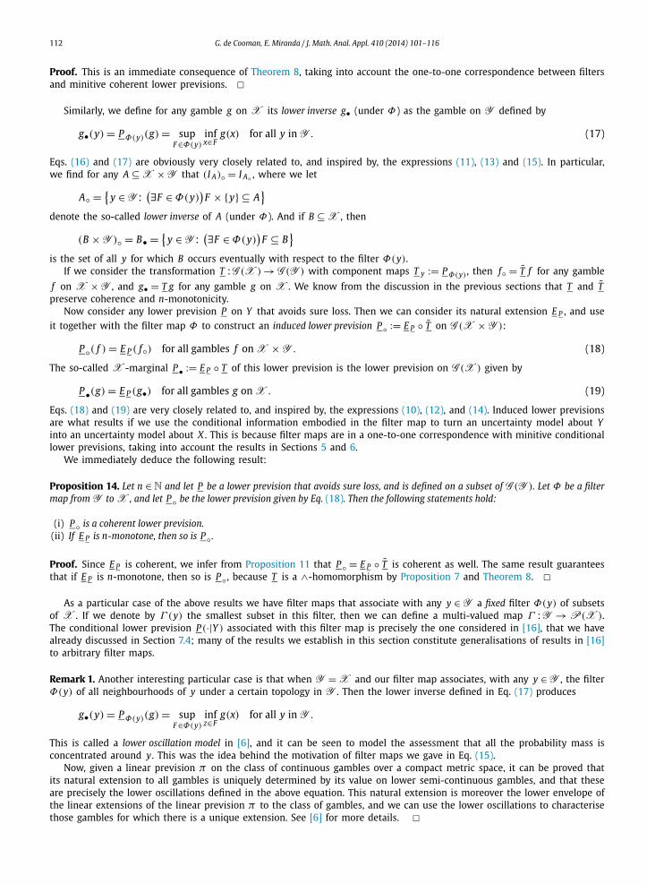
The above result can be summarised by means of the following figure:

P credal set

lower inverse

M(P )

composition with K(Φ)

P ◦credal set

M(P ◦)

The above result allows us to discuss an interesting particular case of filter maps: those associated with ultrafilters.

Definition 11. Let P(X ) denote the power set of X . A subset F of P(X ) is an ultrafilter when it is a filter and moreoverfor any subset A of X , either A or Ac belongs to F .

Similarly to filters, ultrafilters are in a one-to-one correspondence to {0,1}-valued finitely additive probabilities. If thecorresponding filter is fixed, then there is some x ∈ X such that A ∈ F if and only if x ∈ A, and the associated linearprevision corresponds to the degenerate probability measure on x; on the other hand, if the filter is free (i.e., it has nominimal element) then the associated probability is finitely additive but not countably additive.

Any filter of subsets of X can be obtained as the intersection of the ultrafilters that include it [19, Theorem 3.6.6];taking this into account, if we define

K1(Φ) := {K ∈K(Φ): K (y, A) ∈ {0,1} ∀y ∈ Y , A ⊆ X

}it is easy to establish the following:

Corollary 16. Let P be a lower prevision that avoids sure loss, and is defined on a subset of G (Y ). Let Φ be a filter map from Y to X ,and let P ◦ be the lower prevision given by Eq. (18). Then P ◦ is the lower envelope of the set{

P K ( f ): P ∈M(P ), K ∈ K1(Φ)}.

114 G. de Cooman, E. Miranda / J. Math. Anal. Appl. 410 (2014) 101–116

Proof. The result follows from Proposition 15 and [19, Theorem 3.6.6], also taking into account the one-to-one correspon-dence between ultrafilters that include Φ and prevision kernels in K1(Φ). �

If we restrict our attention to the X -marginal P • of the lower prevision P ◦ on G (X ×Y ), we can go somewhat further:the following simple proposition is a considerable generalisation of a result mentioned by Wasserman [20, Section 2.4]; seealso [21, Section 2].3 Here, we use the notation C

∫f dμ for the Choquet integral of the gamble f with respect to a

functional μ [1,10].

Proposition 17. Let n ∈N and let P be a lower prevision that avoids sure loss, and is defined on a subset of G (Y ). If E P is n-monotone,then so is P• , and moreover

P •(g) = C

∫g dP • = C

∫g• dE P = E P (g•) for all g ∈ G (X ). (21)

Proof. That P • is n-monotone follows at once from Proposition 14(ii), taking into account that it is a restriction of P ◦ . Toprove Eq. (21), it suffices to prove that the first and last equalities hold, because of Eq. (19). To this end, use that both E Pand P • are n-monotone, and apply [18, p. 56]. �

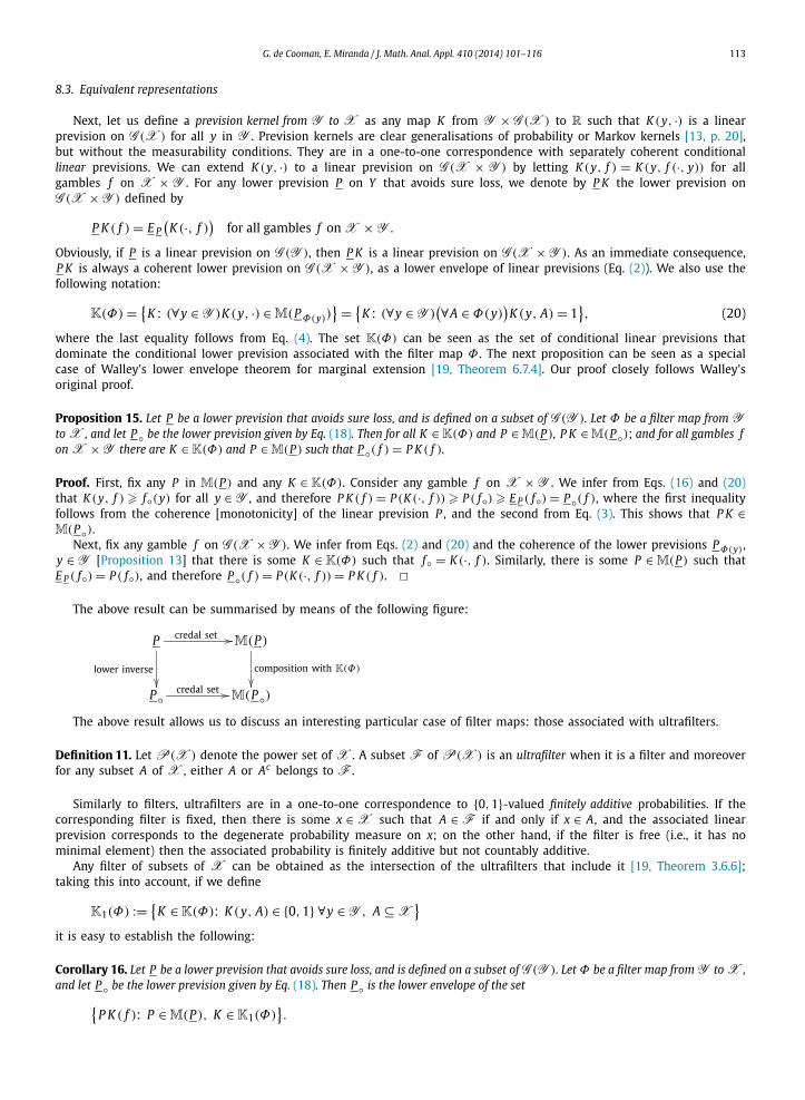
This means that the procedures of natural extension and taking the lower inverse commute, as we represent in thefollowing figure:

Plower inverse of P

natural extension

P •natural extension

E Plower inverse of g

E P (g•) = P •(g)

Now, if the lower prevision P we start with is defined on K ⊆ G (Y ), then it is also useful to consider the lowerprevision P r◦ , defined on the set of gambles

◦K := {f ∈ G (X × Y ): f◦ ∈ K

}as follows:

P r◦( f ) := P ( f◦) for all f such that f◦ ∈ K . (22)

If P is coherent, then of course P r◦ is the restriction of P ◦ to ◦K , because then E P and P coincide on K [see Theo-rem 1(iii)]. We now show that, interestingly and perhaps surprisingly, all the ‘information’ present in P ◦ is then alreadycontained in the restricted model P r◦ .

Proposition 18. Let P be a coherent lower prevision, defined on a set of gambles K ⊆ G (Y ). Then the following statements hold:

(i) P r◦ is the restriction of P ◦ to the set of gambles ◦K , and therefore a coherent lower prevision on ◦K .(ii) The natural extension E P r◦ of P r◦ coincides with the induced lower prevision: E P r◦ = P ◦ .

Proof. (i) It follows from Theorem 1(iii) that E P and P coincide on K . For any f ∈ ◦K , we have f◦ ∈ K and thereforeP ◦( f ) = E P ( f◦) = P ( f◦) = P r◦( f ), also using Eqs. (18) and (22).

(ii) Since P ◦ is coherent [Proposition 14(i)] and coincides with P r◦ on ◦K , we infer from Theorem 1(ii) that E P r◦ � P ◦ .Conversely, consider any gamble f on X × Y , then we must show that E P r◦ ( f ) � P ◦( f ).

Fix ε > 0. If we use the definition of natural extension [for P ] in Eq. (1), we see that there are n in N, non-negativeλ1, . . . , λn in R, and gambles g1, . . . , gn in K such that

f◦(y) − P ◦( f ) + ε

2�

n∑k=1

λk[

gk(y) − P (gk)]

for all y ∈ Y . (23)

It also follows from the definition of the lower inverse f◦ in Eq. (16) that for each y ∈ Y , there is some set F (y) ∈ Φ(y)

such that

infx∈F (y)

f (x, y) � f◦(y) − ε

2. (24)

3 Wasserman considers the special case that P is a probability measure and that g satisfies appropriate measurability conditions, so the right-mostChoquet integral coincides with the usual expectation of g• . See also [15, Theorem 14].

G. de Cooman, E. Miranda / J. Math. Anal. Appl. 410 (2014) 101–116 115

Now define the corresponding gambles hk on X × Y , k = 1, . . . ,n, by

hk(x, y) ={

gk(y) if y ∈ Y and x ∈ F (y),

L if y ∈ Y and x /∈ F (y),

where L is some real number strictly smaller than minnk=1 inf gk , to be determined shortly. Then for any y ∈ Y :

(hk)◦(y) = supF∈Φ(y)

infx∈F

hk(x, y) = supF∈Φ(y)

infx∈F

{gk(y) if x ∈ F (y),

L otherwise= sup

F∈Φ(y)

{gk(y) if F ⊆ F (y),

L otherwise= gk(y),

because L � gk(y) and we can select F = F (y). Hence, (hk)◦ = gk ∈ K and therefore hk ∈ ◦K and P r◦(hk) = P (gk). This,together with Eqs. (23) and (24), allows us to infer that

f (x, y) − P ◦( f ) + ε �n∑

k=1

λk[hk(x, y) − P r◦(hk)

]for all y ∈ Y and x ∈ F (y).

Moreover, by an appropriate choice of L [small enough], we can always make sure that the inequality above holds for all(x, y) ∈ X × Y (note that once L is strictly smaller than minn

k=1 inf gk decreasing it does not affect P r◦(hk) = P (gk)). Thenthe definition of natural extension [for P r◦] in Eq. (1) guarantees that E P r◦ ( f ) � P ◦( f )−ε. Since this inequality holds for anyε > 0, the proof is complete. �9. Conclusions

The above results show that a number of transformations considered in the literature can all be seen as coherencepreserving transformations of a possibility space, and as a consequence they can be combined with an imprecise probabilitymodel of a certain type in order to produce a model of the same type.

If we want to preserve n-monotonicity, which is necessary in order for a lower prevision to have a representation bymeans of a Choquet integral and for it to be uniquely determined by the restriction to events, we have seen that in adefinite sense, it becomes necessary to work with ∧-homomorphisms, which in this context imply working with minitivelower previsions. We have proved that these minimum preserving lower previsions are in a one-to-one correspondence withfilters of events.

Our results given rise to the consideration of filter maps: maps that assign to any element of the initial space a filterof subsets of the final space, and that are in a one-to-one correspondence with conditional lower previsions that preserven-monotonicity. We have studied them in detail, and have shown that they possess a number of interesting properties: forinstance, they commute with other operations such as taking lower inverses and considering the associated credal sets. Indoing this, we have extended a number of results from the literature.

As future lines of research, we would like to point out the application of coherence preserving mappings and filter mapsin decision making, as well as the investigation of their connection with other models, such as p-boxes or (fuzzy) set-valuedrandom variables.

Acknowledgments

The research in this paper has been supported by the SBO project 060043 of the IWT-Vlaanderen and by projectMTM2010-17844.

References

[1] Gustave Choquet, Theory of capacities, Ann. Inst. Fourier 5 (1953–1954) 131–295.[2] Gert de Cooman, Dirk Aeyels, Supremum preserving upper probabilities, Inform. Sci. 118 (1999) 173–212.[3] Gert de Cooman, Filip Hermans, Imprecise probability trees: Bridging two theories of imprecise probability, Artificial Intelligence 172 (11) (2008)

1400–1427.[4] Gert de Cooman, Filip Hermans, Erik Quaeghebeur, Imprecise Markov chains and their limit behaviour, Probab. Engrg. Inform. Sci. 23 (4) (2009)

597–635.[5] Gert de Cooman, Enrique Miranda, Symmetry of models versus models of symmetry, in: W.L. Harper, G.R. Wheeler (Eds.), Probability and Inference:

Essays in Honor of Henry E. Kyburg, Jr., King’s College Publications, 2007, pp. 67–149.[6] Gert de Cooman, Enrique Miranda, The F. Riesz representation theorem and finite additivity, in: Didier Dubois, María Asunción Lubiano, Henri Prade,

María Ángeles Gil, Przemyslaw Grzegorzewski, Olgierd Hryniewicz (Eds.), Soft Methods for Handling Variability and Imprecision, in: Adv. Soft Comput.,Springer, 2008, pp. 243–252.

[7] Gert de Cooman, Erik Quaeghebeur, Enrique Miranda, Exchangeable lower previsions, Bernoulli 15 (3) (2009) 721–735.[8] Gert de Cooman, Matthias C.M. Troffaes, Enrique Miranda, n-Monotone exact functionals, J. Math. Anal. Appl. 347 (2008) 143–156.[9] Morris H. DeGroot, Mark J. Schervisch, Probability and Statistics, fourth edition, Pearson, 2011.

[10] Dieter Denneberg, Non-Additive Measure and Integral, Kluwer, Dordretch, 1994.[11] Didier Dubois, Henri Prade, Possibility Theory – An Approach to Computerized Processing of Uncertainty, Plenum Press, New York, 1988.[12] Filip Hermans, Gert de Cooman, Characterisation of ergodic upper transition operators, Internat. J. Approx. Reason. 53 (4) (2012) 573–583.[13] Olav Kallenberg, Foundations of Modern Probability, second edition, Probab. Appl., Springer, 2002.

116 G. de Cooman, E. Miranda / J. Math. Anal. Appl. 410 (2014) 101–116

[14] Isaac Levi, The Enterprise of Knowledge. An Essay on Knowledge, Credal Probability, and Chance, MIT Press, Cambridge, 1983.[15] Enrique Miranda, Inés Couso, Pedro Gil, Approximation of upper and lower probabilities by measurable selections, Inform. Sci. 180 (8) (2010)

1407–1417.[16] Enrique Miranda, Gert de Cooman, Inés Couso, Lower previsions induced by multi-valued mappings, J. Statist. Plann. Inference 133 (1) (2005) 177–197.[17] Damjan Škulj, The use of Markov operators to constructing generalised probabilities, Internat. J. Approx. Reason. 52 (9) (2011) 1392–1408.[18] Peter Walley, Coherent lower (and upper) probabilities, Statistics Research Report 22, University of Warwick, Coventry, 1981.[19] Peter Walley, Statistical Reasoning with Imprecise Probabilities, Chapman and Hall, London, 1991.[20] Larry A. Wasserman, Belief functions and statistical inference, Canad. J. Statist. (La Revue Canadienne de Statistique) 18 (3) (1990) 183–196.[21] Larry A. Wasserman, Prior envelopes based on belief functions, Ann. Statist. 18 (1) (1990) 454–464.