Embed Size (px)
Citation preview

HAL Id: hal-01877835https://hal-mines-albi.archives-ouvertes.fr/hal-01877835
Submitted on 14 Mar 2019
HAL is a multi-disciplinary open accessarchive for the deposit and dissemination of sci-entific research documents, whether they are pub-lished or not. The documents may come fromteaching and research institutions in France orabroad, or from public or private research centers.
L’archive ouverte pluridisciplinaire HAL, estdestinée au dépôt et à la diffusion de documentsscientifiques de niveau recherche, publiés ou non,émanant des établissements d’enseignement et derecherche français ou étrangers, des laboratoirespublics ou privés.
Lowering Energy Spending Together With Compression,Storage, and Transportation Costs for Hydrogen
Distribution in the Early MarketDidier Grouset, Cyrille Ridart
To cite this version:Didier Grouset, Cyrille Ridart. Lowering Energy Spending Together With Compression, Storage,and Transportation Costs for Hydrogen Distribution in the Early Market. Catherine Azzaro-Pantel.Hydrogen supply chains : design, deployment and operation, Elsevier, pp.207-270, 2018, 978-0-12-811197-0. �10.1016/B978-0-12-811197-0.00006-3�. �hal-01877835�

Lowering energy spending together with compression, storage and transportation costs for hydrogen distribution in the early market
D GROUSET, C RIDART
1 Author version of the paper submitted as a contribution for Chapter 6 of the book:
‘‘Design, deployment and operation of a hydrogen supply chain”, Coord. Catherine Azzarro-Pantel https://doi.org/10. 1016/B978-0-12-811197-0. 00006-3 – Elsevier ed. - Copyright © 2018.
VaBHyoGaz3_2.1.S05_vC_2018_05_23 – Mai 2018
Chapter 6
Lowering energy spending together with compression, storage and transportation costs for hydrogen distribution in the early market
1
Didier Grouset a, 2
, Cyrille Ridart b a RAPSODEE, UMR CNRS 5302. IMT Mines Albi, campus Jarlard, 81000 ALBI, France
b HERA / ALBHYON, Technopole Innoprod, rue Pierre Gilles de Gennes, 81000 ALBI, France
Abstract
This present paper is dedicated to the optimization of cost and energy consumption for compression, transportation and storage of hydrogen for vehicle refueling in the current hydrogen emerging market. So it considers only small refueling stations (20 to 200 kg/day) and currents costs. It considers 2 cases: the case of a refueling station on the site of the hydrogen production and the case of a production unit supplying hydrogen to several distant refueling stations. In the case of production and distribution located on the same site, no transportation has to be considered and the energy consumption is mainly due to hydrogen compression and cooling. In a reference case corresponding to good current practices, the study calculates an energy need at 3.5 or 4.4 kWh per kg of hydrogen transferred to car tank at respectively 35 or 70 MPa. It then shows that this need can be reduced by more than 25 % when judiciously using 4 or 5 stages of buffers organized in a pressure cascade for the filling of a tank at 70 MPa. Whereas the total volume of the staged buffers is higher than the volume of an only very high pressure buffer (VHPB), the investment cost is only slightly higher; then the energy saving results in short payback times for the extra investments in staged buffers. In the case of a production unit supplies hydrogen to several distant hydrogen refueling stations, energy for transportation by truck and for re-compression on the distribution site must be added. Current offsite distribution practices are used as a reference case: it considers the transportation of hydrogen in 20 MPa steel bottle bundles or trailer tubes and the re-compression of all the hydrogen to the VHPB. To lower the energy spending, solutions are proposed and quantified, such as using small transportable containers of higher pressure light composite bottles and by-passing of the compressor as much as possible. Energy needs and CO2 emissions are estimated and compared for the reference case and the innovative cases. The study shows that, even if the investment in composite bottles is high, the resulting overall cost is definitely lower and CO2 emissions can largely be decreased. The size effect appears very important: cost decreases by 60% from 20 to 200kg/day. 364 words
________________________________________________________________________________________
Key words:
Hydrogen, compression, storage, transportation, energy, CO2 emissions, costs
________________________________________________________________________________________________________
1 Acknowledgement: This work is a part of the VABHYOGAZ3 project supported by the French “Programme d’Investissements
d’Avenir’’ under supervision of ADEME, the French Energy and Environment Agency. The project is conducted by HERA France
office ALBHYON, in partnership with TRIFYL, HP Systems, EMTA (VEOLIA group) and the IMT Mines-Albi RAPSODEE
Research Center. The VABHYOGAZ3 project considers hydrogen production from biogas with production units ranging from 100 to
800 kg/day to deliver hydrogen to several distribution units of 20 to 200 kg/day located within a distance less than 100 km from the
production unit. The authors are grateful towards the ADEME for its support to this project. 2 Corresponding author: [email protected], [email protected]

Lowering energy spending together with compression, storage and transportation costs for hydrogen distribution in the early market
D GROUSET, C RIDART
2 Author version of the paper submitted as a contribution for Chapter 6 of the book:
‘‘Design, deployment and operation of a hydrogen supply chain”, Coord. Catherine Azzarro-Pantel https://doi.org/10. 1016/B978-0-12-811197-0. 00006-3 – Elsevier ed. - Copyright © 2018.
VaBHyoGaz3_2.1.S05_vC_2018_05_23 – Mai 2018
Introduction
1. Hydrogen supply chain and energy requirements
Future developments of hydrogen fuel cell vehicles promise an important decrease in the final spent energy
and in greenhouse gas and pollutant emissions from transportation. This is mainly due to the qualities of
hydrogen fuel cells: high efficiency for chemical to electric conversion, no other product than water, no
pollutant emission, no noise… Nevertheless, the overall energy chain has to be considered to quantify the
benefits of hydrogen as a new energy carrier: from the primary energy used for hydrogen production to the
final step of the useful energy spent for the vehicle movement. Indeed, great care has to be taken so that the
decrease in the final spent energy does not induce too large an increase in the energy spent in the
intermediate steps of hydrogen production, storage, transportation and distribution.
Nowadays, everybody would agree that the primary energy for the future large production of hydrogen
energy has to be renewable: through electrolysis of renewable electricity (photovoltaic, wind, hydraulic),
through reforming of renewable hydrocarbons (e;g; biogas), through biomass gasification and possibly
others.
An advantage of hydrogen is that sources for its production are numerous and largely widespread over the
world, so that its production is possible nearly everywhere and close to its valorization location.
Transportation can then be avoided or reduced to small distances: costs and energy spending can be saved
for hydrogen energy. This is not the case for fossil fuels which will have to be transported over longer and
longer distances between their production sites and their distribution sites: several thousands of kilometers,
resulting into losses of energy and CO2 emissions; for example, a loss of about 20% of the energy content of
natural gas for its pipe line transportation over 5000 km! Currently, with few hydrogen production sites and
truck transportation other distances of several hundred km, similar energy spending and CO2 emissions can
be encountered with the industrial hydrogen or the energy hydrogen for the very early market; but solutions
under development will eliminate this problem, as shown in this paper.
Compression of hydrogen for its storage has also to be considered with care; indeed it is a high energy
consuming operation as pointed out by M. Klell & al. [1]. Hydrogen is a very light and bulky gas and its
compression requires a lot of energy: as the green curve shows in figure 1, the isothermal compression work
from 0.1 MPa to 100 MPa represents more than 7% of the hydrogen energy content (7.2% of LHVH2,
hydrogen low heating value which is 120 MJ/kg). One should keep in mind that this only represents the
mechanical energy transferred to hydrogen in the ideal isothermal compression and efficiencies losses have
to be added: any warming of hydrogen during compression, friction in the compressor or inefficiency of the
electric motor will increase the spent energy. Moreover, the efficiency for electric energy production from
chemical energy into should also be considered (50% in best cases). Thus if not processed with care, the
compression step could be responsible of more than a 20% loss of the hydrogen electric energy potential.
However, compressing hydrogen higher than 70 MPa is a necessity to refill vehicle tanks at that pressure! On
the other hand using liquid hydrogen would not be a better solution, as the violet curve of the same figure
shows even higher energy needs for the liquefaction of hydrogen... Hopefully, as shown in this paper, some
good practices can lower this energy spend.
The different steps of hydrogen production, compression, transportation are linked together by the storage for
which different technologies are now matured. Only high pressure gaseous storage is considered in this
paper. Steel bottles or tubes (type 1 vessels) are being used for a very long time and are now challenged in
cost, especially for very high pressure, by composite material bottles with an aluminum or plastic internal

Lowering energy spending together with compression, storage and transportation costs for hydrogen distribution in the early market
D GROUSET, C RIDART
3 Author version of the paper submitted as a contribution for Chapter 6 of the book:
‘‘Design, deployment and operation of a hydrogen supply chain”, Coord. Catherine Azzarro-Pantel https://doi.org/10. 1016/B978-0-12-811197-0. 00006-3 – Elsevier ed. - Copyright © 2018.
VaBHyoGaz3_2.1.S05_vC_2018_05_23 – Mai 2018
liner (type 3 or 4 vessels). This study quantifies the savings induced by the light weight of these storage
bottles.
Figure 1: specific mass and minimum works for compression and liquefaction of hydrogen as a function of pressure, as in [1]
Finally, concerning the distribution, many studies have been conducted during the last 2 decades concerning
the most secure way to fill hydrogen car tanks. Some of them have been realized by international teams that
included researchers from different car companies, gas companies, hydrogen technology companies and
research centers and were reported, for example, during the successive NHA (National Hydrogen
Association) congresses, as by Schneider & al. [2] or by Maus & al. [3]. They resulted in the release in July
2014 of a last version of the SAE-J6201 standard [4] for fueling protocols for gaseous hydrogen vehicles
under 35 or 70 MPa pressures on which are based all current and future refueling stations.
The contribution of compression and storage in the investment cost of hydrogen refuelling station (HRS) is
known to be high: following [5], it is one half to two thirds the cost, according the HRS size. Thus it seems
important to focus on these costs to understand how they contribute to the overall cost of the delivered
hydrogen.
2. Refueling principles: current practices
In current practices for a rapid filling [6], [7], the vehicle tanks are filled at their nominal pressure simply by
pouring available hydrogen from a cascade of buffers, as shown on the figure 2. These buffers have been
previously filled with hydrogen at a higher pressure by a compressor connected to the hydrogen production
unit, or to a mass intermediate storage. A regulation valve controls the mass flow rate delivered to the tank
and the pressure raise in the tank, according to the SAE-J2601 standard [4].
The performances metrics of an HRS are: delivering pressure, time for filling a tank and delivering capacity
at the peak hour.

Lowering energy spending together with compression, storage and transportation costs for hydrogen distribution in the early market
D GROUSET, C RIDART
4 Author version of the paper submitted as a contribution for Chapter 6 of the book:
‘‘Design, deployment and operation of a hydrogen supply chain”, Coord. Catherine Azzarro-Pantel https://doi.org/10. 1016/B978-0-12-811197-0. 00006-3 – Elsevier ed. - Copyright © 2018.
VaBHyoGaz3_2.1.S05_vC_2018_05_23 – Mai 2018
• Delivering pressure: two standards, 35 and 70 MPa, coexist for hydrogen vehicle tank pressure.
• Time for refueling: the pressure difference between the very high pressure of the buffer storage (e;g;
45 or 90 MPa) and the tank ensures rapid filling. A cooling of the hydrogen is sometime
implemented: it is recommended by SAE-J2601 to allow a filling within 3 minutes in nearly all
conditions of ambient temperature and initial tank pressure. Small hydrogen refueling stations do
not refrigerate hydrogen and cannot guarantee a min refueling.
• The peak hour performance relies mainly on the mass of hydrogen stored in the HP buffers and only
incidentally on the mass flow rate of the compressor. In fact this results from a cost optimization:
compressors are expensive and it is cheaper having a small compressor working nearly all day long
to fill buffers than a large compressor with the possibility to fill directly the tank within a few
minutes.
Figure 2: schematic view of the equipment used for filling hydrogen vehicle HP tanks
Bulk storage is considered as a basic feature of an HRS: when connected to a hydrogen pipe line (a 17.2 MPa
bulk storage is considered in [6]), when supplied by trucked trailers [8], or with onsite production (between
20 and 35 MPa in [7]).
The buffer storage is usually made of several vessels which can be isolated and connected successively to the
vehicle tank. They are always connected to the tank in the same order and the compressor fills in priority the
highest pressure buffer (number 3 in fig. 2), so that the buffers finally form a pressure cascade, from 35 to 90
MPa for a 70 MPa refueling as recommended in [7].
3. Content and objectives of this paper
The present paper is dedicated to the optimization of cost and of energy consumption of compression,
transportation and storage for hydrogen distribution in the current early hydrogen energy market.
Specific emphasis is put on energy needs: whereas costs have often been studied, quantitative information
concerning energy consumption are in fact less available. For example [7] writes as well that energy
consumption of HRSs are unknown; [9] reports variations by a factor of 10 for compression energy
consumption; [10] gives more general figures for compression or liquefaction energies.
This chapter aims as well to present the equations necessary to calculate the basic design features of
compression, storage and transportation equipment and to evaluate cost and energy. Simple models are
formulated, together with their simplifying assumptions, so that it becomes possible to transpose the
approach to specific cases other that those discussed here.
This chapter is connected with current or in the near future implementations, in the emerging market of
hydrogen energy, especially in France. Thus it only considers small HRSs (from 20 to 200 kg/day) whereas

Lowering energy spending together with compression, storage and transportation costs for hydrogen distribution in the early market
D GROUSET, C RIDART
5 Author version of the paper submitted as a contribution for Chapter 6 of the book:
‘‘Design, deployment and operation of a hydrogen supply chain”, Coord. Catherine Azzarro-Pantel https://doi.org/10. 1016/B978-0-12-811197-0. 00006-3 – Elsevier ed. - Copyright © 2018.
VaBHyoGaz3_2.1.S05_vC_2018_05_23 – Mai 2018
most other papers are concerned with long term perspectives for a developed hydrogen market with large
HRSs: 850, 1000 and 1330 kg/day in [6], 250 kg/day in [8]… The cost generated here are for current
implementations: they are issued from commercial consultations during 2015 and 2016 and no reduction
factor has been applied for mass production which will undoubtedly occur in the next decade, especially for
composite pressure bottles, but also for compressors.
First, in sections A and B general technical and economic data concerning compression and storage, the way
they were obtained, or how to calculate them, is presented and discussed.
Then 2 different cases are studied: in section C, the case of a refueling station on the site of the hydrogen
production is analyzed. Then the energy spent for the hydrogen distribution is linked to the compressor
consumption, to the cooling of the compressor and, if any, to the cooling of hydrogen before being delivered
to the vehicle tank.
In section D, the case of a production unit providing hydrogen to several distant refueling stations is
considered. The different steps leading to hydrogen distribution are described in the current practice and
when using better practice, evaluating for each the energy consumption, CO2 emission, investment cost and
operation cost in order to estimate globally for these steps (excluding the production step and the final
distribution step), the total cost of ownership (TCO) in €/kg, the specific consumption in kWh/kgH2 and
specific emission in tCO2/tH2.
A – Technical data for compression and storage
This section presents general technical data which are used in the following sections. There will also be a
discussion of these data with respect to data used by other auteurs in similar papers, where appropriate.
1. Thermodynamic data for hydrogen
Hydrogen in not a perfect gas and correct thermodynamic data have to be used in order to get good
estimations of heat and work exchanged during heating, cooling or compression. More precisely, evolutions
of specific mass�, of specific internal energy � or enthalpy � or heat capacity ��, ��, and of entropy with
temperature and pressure �, �� are needed. Different sources can be used for this. [1] gives interesting
information and �, � diagrams at low temperature. [4] gives, in its appendix, regressions for �, �, � and �� as functions of �, ��. Lemmon & al [11] from NIST derived a state equation for hydrogen where the
compressibility factor �, �� is calculated through a 9 term regression, each term needing 3 coefficients,
according to the formula:
��. ��
The accuracy of this regression is very good: 0.15%, in a large range of � (up to 200 MPa) and � (150 to
1000 K). Then, knowing �, �� allows a calculation of � and �.
Calculations in this paper also use hydrogen thermodynamic data available for the chemical data webbook
published by NIST [12]. From the values of ��, �� read in the tables, �, �� can be calculated and
polynomial regressions, simpler than eq.1, have been derived. NIST webbook also gives values for � and �, , ��, �� used in this paper. An example of the result for �, �� variation with � ranging from 0.1 to
90 MPa is given in the figure 3: �, �� increases from 0,99 at ambient pressure to 1.63 at 90 MPa at � =273
K.

Lowering energy spending together with compression, storage and transportation costs for hydrogen distribution in the early market
D GROUSET, C RIDART
6 Author version of the paper submitted as a contribution for Chapter 6 of the book:
‘‘Design, deployment and operation of a hydrogen supply chain”, Coord. Catherine Azzarro-Pantel https://doi.org/10. 1016/B978-0-12-811197-0. 00006-3 – Elsevier ed. - Copyright © 2018.
VaBHyoGaz3_2.1.S05_vC_2018_05_23 – Mai 2018
Figure 3: variation of hydrogen compressibility factor ��, �� for T=273K.
2. Compression work, isothermal or adiabatic
The useful work developed by a compressor is equal to the work of the pressure forces during the volume
decrease of the compressed hydrogen; pressure and volume are linked through the gas state equation; thus for
a mass � or mole number � the compression work is:
������ = − � � ∗ ����
� �!= − � �, �� �"�� ∗ ��
��� �!
= −� ∗ " #$ � �, �� ∗ �� ∗ ����
� �!��. %�
As hydrogen has the lowest molar mass # of all gases, the mass compression work will be the highest.
Moreover, hydrogen is a non-perfect gas with &%�, �� > �, which means that the compression work will
be higher than for a perfect gas or for methane which is a non-perfect gas with (&)�, �� < �. The high
values of �, �� lead to a significant increase of the useful work with respect to a perfect gas.
In the case of an isothermal compression of a perfect gas, eq.2 can easily be integrated and leads to the useful
compression energy, reference energy as the lowest possible:
�+,-��.�/�,��.���- = −� ∗ " #$ ∗ �! � �����
� �!= � ∗ " #$ ∗ �! ∗ �� 0�� �!$ 1��. 2�
For hydrogen or any non-perfect gas, the integral has to be calculated step by step, but the result can be
expressed as:
�+,-��.�/�,&% = &%!�3333333 ∗ �+,-��.�/�,��.���-��. )� Where the coefficient &%!�3333333 represents the real gas effect, comprised between &%�!, �!� and &%4��, ��5. The result, divided by the hydrogen LHV, is plotted in fig. 1 as a function of �� for �! = �bar.
Furthermore compressing a gas leads to an increase in its temperature, increasing its volume and thus
increasing also the compression work. If the compression is adiabatic, temperature and pressure are linked, so
that the final temperature and the isentropic compression work of a perfect gas can be expressed as:

Lowering energy spending together with compression, storage and transportation costs for hydrogen distribution in the early market
D GROUSET, C RIDART
7 Author version of the paper submitted as a contribution for Chapter 6 of the book:
‘‘Design, deployment and operation of a hydrogen supply chain”, Coord. Catherine Azzarro-Pantel https://doi.org/10. 1016/B978-0-12-811197-0. 00006-3 – Elsevier ed. - Copyright © 2018.
VaBHyoGaz3_2.1.S05_vC_2018_05_23 – Mai 2018
�+��-.,�+�,��.���- = � ∗ " #$ ∗ �! ∗ 66 − � ∗ 70�� �!$ 168�6 − �9��. :� �� = �! ∗ 0�� �!$ 168�6 ��. ;�
For hydrogen, non-perfect gas, the result can be written as:
�+��-.,�+�,&% = ′&%!�3333333 ∗ �+��-.,�+�,��.���-��. =� Eq.3 and eq.5 clearly show that the main parameter is the pressure ratio .� = �� �!$ and also that the lower
the initial temperature �!, the lower is the compression work. In the case of large compression ratios, the
isentropic temperature increase can be large and the isentropic compression work will be much larger than
the isothermal compression work. For example, for a compression from 2 MPa to 45 MPa, the pressure ratio
is 22.5 and
��,+��-.,�+� = �! ∗ %%. :�6>�6 = %. )2 ∗ �!, so: �+��-.,�+�,��.���- = �. ;� ∗�+,-��.�/�,��.���-. It is clear that cooling the gas and the compressor is necessary to lower the compression work. Splitting the
compression into several successive intercooled stages is also beneficial.
4. Compression efficiency
Moreover, frictions and efficiency losses also increase the gas temperature and the electric power needed by
the compressor. The question is how to estimate compressor efficiency? A lot of parameters influence the
efficiency and first of all is the compressor technology. Several matured technologies can be found for
hydrogen compression: reciprocating compressors, diaphragm compressors and pneumatic or hydraulic
boosters.
It is not the purpose of this paper to present details about these safe and matured technologies, but to focus on
some information concerning the energy needs in compression. The diaphragm compressor will have better
energy efficiency, defined as the ratio between the energy transferred to the compressed hydrogen and the
consumed electric energy:
• The friction of pistons in the booster cylinders generates higher losses than the deformation of the
diaphragm. It can also be understood that frictions will be relatively higher for smaller capacity
compressors.
• Losses occur in the compression of the working fluid (oil or air) in boosters, and these losses will be
more elevated for compressed air than for compressed oil; while the diaphragm compressor crank
benefits of a direct electric drive.
• In case of low or medium charge of the compressor (e.g. when the storage pressure is only at 5 or 20
MPa for a nominal pressure of 45 or 90 MPa), the diaphragm compressor will adapt and will need
less energy, whereas the booster always consumes the same energy: the oil has been compressed up
to 20 MPa (or the air compressed up to 0.8 MPa) and the extra energy will be lost.
It is important to define the way to calculate the efficiency. [13] recommends defining efficiency with respect
to isentropic (or adiabatic) work and reports isentropic efficiencies in the range of 86 to 92% for large
reciprocating compressors. But the compressors considered for hydrogen distribution in general and
specifically in the present study are really smaller. [6], [7] and [8] follow this recommendation and use
isentropic efficiency. [7] uses a formula from chemical processes [14] for the variation of isentropic
efficiency with the pressure ratio and assumes that all efficiency losses contribute to increase hydrogen
enthalpy (no external losses), which again is acceptable for large non cooled compressors. [7] and [8] are

Lowering energy spending together with compression, storage and transportation costs for hydrogen distribution in the early market
D GROUSET, C RIDART
8 Author version of the paper submitted as a contribution for Chapter 6 of the book:
‘‘Design, deployment and operation of a hydrogen supply chain”, Coord. Catherine Azzarro-Pantel https://doi.org/10. 1016/B978-0-12-811197-0. 00006-3 – Elsevier ed. - Copyright © 2018.
VaBHyoGaz3_2.1.S05_vC_2018_05_23 – Mai 2018
using a 65% isentropic efficiency. [6] underlignes the lack of experimental data and a large dispersion, by a
factor of 10, of the few compressor consumption data reported in [9] for hydrogen distribution, while DOE
estimates in 2013 consumptions from 2 to 4 kWh/kgH2 for 35 MPa refueling with an efficiency about 65%
and targets 80% in 2020.
Indeed, efficiency varies greatly with the compressor technology, its capacity, its nominal pressure ratio and
the current pressure ratio… It is also important to consider each single stage, as recommended in [10] and
followed in [7], as intercooling considerably reduces the final temperature and isentropic power.
Yet, compressors always exchange heat with the ambience; for small compressors this can be significant with
respect to the necessary heat to cool the compressed hydrogen, while for medium or large capacities, boosters
or diaphragm compressor heads are equipped with cooling jackets. Isothermal work is the reference as the
lowest needed to compress a gas and thus its calculation relevant. Nevertheless, cooling is never totally
efficient, leaving a residual heating of hydrogen during compression. Thus it seems relevant to calculate the
efficiency with respect to both isothermal and isentropic power; in this study, the average of isothermal and
isentropic works for each stage is used (as eq.5 and eq.7). Thus the electric power needed for each stage of a
compressor is calculated as follows:
?�����,��&% = ���,�� �@ +,-��.�/�,&% A�@ +��-.,�+�,&%�/%��. C� Indeed very large variations in efficiency are found; for small capacity pneumatic boosters, the efficiency can
be very low: for example for compressing 10 kg/day from 5 to 45 MPa an efficiency of 10 to 15% has been
calculated according to supplier data; hydraulic boosters are slightly higher: 15 to 20% has been calculated.
On the opposite end of the spectrum, for a large 2 stage cooled diaphragm compressor, compressing at its
nominal point of 850 kg/day from 1.2 to 25 MPa at 27°C and consuming 73,5 kW, an efficiency of 59% has
been calculated following eq.8. With respect to isentropic power only, which is 48 kW with two stages, the
isentropic efficiency is 65.2%, which is fully coherent with [8] and [6]. Forgetting the 2 stages and
considering only 1, would mislead to an isentropic power of 62 kW and an apparent efficiency of 84.5%.
Furthermore it is known that large compressors have a better efficiency than small ones and in this study
considering cooled diaphragm compressors, while more data from suppliers would be needed, the effect of
capacity on efficiency will be calculated by a power law according to eq.9, presented in fig. 4.
��,�� = ��,��,!�@ �@ !$ ����,��,! = ;!%�@ ! = C:!EF �/G$ � = !. ���. H�
Lowering energy spending together with compression, storage and transportation costs for hydrogen distribution in the early market
D GROUSET, C RIDART
9 Author version of the paper submitted as a contribution for Chapter 6 of the book:
‘‘Design, deployment and operation of a hydrogen supply chain”, Coord. Catherine Azzarro-Pantel https://doi.org/10. 1016/B978-0-12-811197-0. 00006-3 – Elsevier ed. - Copyright © 2018.
VaBHyoGaz3_2.1.S05_vC_2018_05_23 – Mai 2018
Figure 4: estimated effect of nominal capacity of a cooled diaphragm compressor on its stage efficiency
5. Cooling needs
Compressor heads have to be cooled to keep the compression as isothermal as possible; hydrogen has to be
cooled at the exit of each compression stage as well. The cooling power to develop can easily be estimated
according to the thermodynamics law, which teaches that during a fluid transformation, the enthalpy
variation is equal to the sum of the heat and work exchanged with the outside of the system: ∆& = �AJ��. �!�In the case of a perfect gas, the enthalpy only depends on temperature; as the gas recovers its initial
temperature at the end of the compression + cooling process, then: �� = �!∆&��.���- = ! and J�,,�+�F = −��,����. ���This equation shows that a heat equivalent to the whole compression work provided to the gas has to be
extracted from the system. Moreover, all losses in compressor, drive and electric motor convert into heat and
also have to be extracted. Then, it is a cooling power equivalent to the electric power which has to be
provided, through exchange with a cooling fluid and through natural convection with the ambient air.
Now, hydrogen is not a perfect gas and the variation of its enthalpy with temperature and pressure can be
calculated using data from [12]; then according to eq.10 the cooling needs will slightly decrease due to the
variation of enthalpy with pressure: J�,,�+�F,&% = −��,��,&% A��&%4�!, ��5 − �&%�!, �!����. �%�
Cooling is assumed to be provided through a frigorific machine with a performance coefficient (K?�,,�+�F
of 3 and thus the electrical power of this machine is:
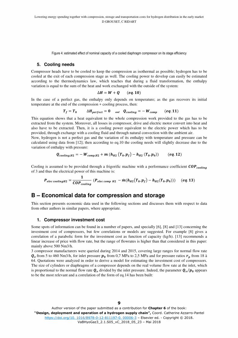
?�����,,�+�F&% = �(K?�,,�+�F ?�����,��&% − �@ �&%4�!, ��5 − �&%�!, �!�����. �2� B – Economical data for compression and storage
This section presents economic data used in the following sections and discusses them with respect to data
from other authors in similar papers, where appropriate.
1. Compressor investment cost
Some spots of information can be found in a number of papers, and specially [6], [8] and [13] concerning the
investment cost of compressors, but few correlations or models are suggested. For example [8] gives a
correlation of a parabolic form for the investment cost as function of capacity (kg/h). [13] recommends a
linear increase of price with flow rate, but the range of flowrates is higher than that considered in this paper:
mainly above 500 Nm3/h.
3 compressor manufacturers were queried during 2014 and 2015, covering large ranges for normal flow rate J� from 5 to 460 Nm3/h, for inlet pressure �! from 0,7 MPa to 2,5 MPa and for pressure ratios .� from 18 à
64. Quotations were analyzed in order to derive a model for estimating the investment cost of compressors.
The size of cylinders or diaphragms of a compressor depends on the real volume flow rate at the inlet, which
is proportional to the normal flow rate J� divided by the inlet pressure. Indeed, the parameter J� �!⁄ appears
to be the most relevant and a correlation of the form of eq.14 has been built:
Lowering energy spending together with compression, storage and transportation costs for hydrogen distribution in the early market
D GROUSET, C RIDART
10 Author version of the paper submitted as a contribution for Chapter 6 of the book:
‘‘Design, deployment and operation of a hydrogen supply chain”, Coord. Catherine Azzarro-Pantel https://doi.org/10. 1016/B978-0-12-811197-0. 00006-3 – Elsevier ed. - Copyright © 2018.
VaBHyoGaz3_2.1.S05_vC_2018_05_23 – Mai 2018
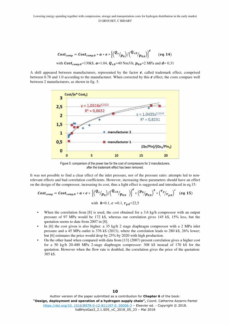
(,-�,�� = (,-�,��,! ∗ / ∗ � ∗ M0J� �!$ 1 0J�,! �!,!$ 1$ N� ��. �)� with (,-�,��,!=130k$, /=1.04, J�,!=40 Nm3/h, �!,!=2 MPa and �= 0,31
A shift appeared between manufacturers, represented by the factor e, called trademark effect, comprised
between 0.78 and 1.0 according to the manufacturer. When corrected by this e effect, the costs compare well
between 2 manufacturers, as shown in fig. 5.
Figure 5: comparison of the power law for the cost of compressors for 2 manufacturers, after the trademark effect has been removed.
It was not possible to find a clear effect of the inlet pressure, nor of the pressure ratio: attempts led to non-
relevant effects and bad correlation coefficients. However, increasing these parameters should have an effect
on the design of the compressor, increasing its cost, thus a light effect is suggested and introduced in eq.15:
(,-�,�� = (,-�,��,! ∗ / ∗ � ∗ M0J� �!$ 1 0J�,! �!,!$ 1$ N� ∗ 0�! �!,!$ 1O ∗ 0.� .�,!$ 1� ��. �:� with O=0.1, � =0.1, .�,!=22,5
• When the correlation from [8] is used, the cost obtained for a 3.6 kg/h compressor with an output
pressure of 97 MPa would be 172 k$, whereas our correlation gives 145 k$, 15% less, but the
quotation seems to date from 2007 in [8].
• In [6] the cost given is also higher: a 35 kg/h 2 stage diaphragm compressor with a 2 MPa inlet
pressure and a 45 MPa outlet is 376 k$ (2013), where the correlation leads to 280 k$, 26% lower;
but [6] estimates the price would drop by 25% by 2020 with high production.
• On the other hand when compared with data from [13] (2007) present correlation gives a higher cost
for a 50 kg/h 20-400 MPa 2-stage diaphragm compressor: 308 k$ instead of 170 k$ for the
quotation. However when the flow rate is doubled, the correlation gives the price of the quotation:
385 k$.

Lowering energy spending together with compression, storage and transportation costs for hydrogen distribution in the early market
D GROUSET, C RIDART
11 Author version of the paper submitted as a contribution for Chapter 6 of the book:
‘‘Design, deployment and operation of a hydrogen supply chain”, Coord. Catherine Azzarro-Pantel https://doi.org/10. 1016/B978-0-12-811197-0. 00006-3 – Elsevier ed. - Copyright © 2018.
VaBHyoGaz3_2.1.S05_vC_2018_05_23 – Mai 2018
2. Cost of pressure vessels
As for compressor investment cost, some information can be found about high pressure vessels cost in a
number of papers, for example [6] [8] and [13], but no model is available.
• [13] considers large steel vessels of 21 kg H2 each under 43 MPa for a price of 843 $/kg (2007, non-
installed).
• [8] considers 100-MPa steel bottles with a capacity of 12 kg for a rather high cost of 1475 $/kg
(2013, +30% for installation).
• [6] reports previous figures from [13] and add others, with lower costs and for higher pressure: for
61 kg at 25 MPa, a 5-kg type-4 bottle container is reported at a cost of 450 $/kg (2007) and at 95
MPa, type-4 12-kg bottles are selected at a cost of 911 $/kg.
It is interesting to note that composite bottles have reached lower costs than steel vessels and will continue to
drop costs with mass production whereas steel vessels will less drop in cost as the technology is matured
since a long time.
3 manufacturers of composite type 3 and type 4 pressure bottles were queried in 2015 and 2016. They
covered a range of bottles with nominal pressures from 20 to 52.5 MPa and volumes from 75 to 500 L. It was
then possible to show that the costs of the composite bottles could fit a correlation based on the nominal
pressure and the mass capacity of the bottles of the following form: (,-O,--�� = � ∗ ��,�O,--���� ∗ �/�/O,--������. �;�With ��,�O,--�� in MPa, �/�/O,--�� =�&%�,�O,--�� ∗ �O,--�� in kg, � = 0.27, � = 0.875 and � = 331€.
When applied to the bottles characteristics of ref [6], the correlation would give a price of 635€/kg = 730$/kg
at 25 MPa and 840€/kg = 965$/kg at 95 MPa. Thus the order of magnitude is correct while the effect of
pressure seems underestimated.
In fact, in [6] at 25 MPa, the bottles were assembled in a container for a larger capacity and the cost should
be compared to costs collected by enquiries for containers varying from 160 to 850 kg. The cost of a
container made of elementary bottles can be expressed as: (,-�,�-/+��. = �� ∗ �P ∗ � ∗ ��,�O,--���� ∗ �/�/O,--������. �=� Where �P is a coefficient relative to the cost of building the frame of the container, the supports of vessels and
their connection, with a value of 1.3 to 1.5 (from quotation analysis, relevant with [13]), � is the number of
vessels necessary for the container capacity requirement and the exponent � reveals the number effect, from
0.90 to 0.94 (from quotations analysis from different suppliers). When applied to the 616 kg container of [6],
the correlation gives a cost of 680€/kg for the assembled container instead of 635€/kg for a single 5 kg bottle:
the number effect has nearly compensated the assembly cost.
These correlations are used in sections C and D without taking into account the cost drop with large quantity
production, which will indubitably occur in the next years.
3. Preliminary considerations and recommendations
At this stage, good practices already appear concerning hydrogen compression:
• Use high �!: as far as possible, produce the hydrogen at the highest pressure, using a high pressure
electrolyzoer or a high pressure reformer and PSA : it is less costly to compress the water feeding
the electrolyser or the biogas at the inlet of the reformer than the hydrogen at the exit. In the
VABHYOGAZ project, the reformer operates at �! =1.5 MPa.

Lowering energy spending together with compression, storage and transportation costs for hydrogen distribution in the early market
D GROUSET, C RIDART
12 Author version of the paper submitted as a contribution for Chapter 6 of the book:
‘‘Design, deployment and operation of a hydrogen supply chain”, Coord. Catherine Azzarro-Pantel https://doi.org/10. 1016/B978-0-12-811197-0. 00006-3 – Elsevier ed. - Copyright © 2018.
VaBHyoGaz3_2.1.S05_vC_2018_05_23 – Mai 2018
• Use low �!: cool the hydrogen the before compression, as far as the compressor accepts it.
Calculations (see later) show that with a (K?�,,�+�F of 3, the hydrogen refrigeration will require
less electric energy than can be spared when compressing hydrogen at lower temperature.
• Cool effectively the compressor heads, so that the compression process be as near as possible to an
isothermal process; consider multiple stage compressor with intercooling to lower compression ratio
of each stage and isentropic heating.
• Choose best compression technology: diaphragm compressors are more effective than boosters
• Prefer large scale units: it is difficult to reach good compressor efficiency in small production or
distribution units.
• Choose an effective cooling system to cool compressor heads and hydrogen.
C - Case of H2 distribution on the production site
When hydrogen production and distribution are located on the same site, there is no transportation to be
considered and the energy requirements are mainly from the compression and associated cooling of the
hydrogen.
1. Current practices for refueling: energy costs for reference cases
In the current practice referring to figure 2, during the filling of successive vehicle tanks, the buffers
numbered 1, 2 and 3 are always connected in the same order to the vehicle and they are then refilled by the
compressor in the opposite order: with a priority to the highest pressure buffer, number 3. Then, when buffer
number 3 has recovered its nominal pressure, it is the turn of the buffer number 2 to be refilled by the
compressor up to its nominal pressure. And finally it will be the turn for buffer number 1 to be refilled. Even
though [7] writes the compressor refills the buffers in the order they are filling the tanks, i.e. number 1 first,
this practice seems not being implemented.
Indeed, refilling first the buffer number 3 is useful for the peak hour performance: this highest pressure buffer
will recover its nominal pressure (45 MPa or 90 MPa) within the shortest time; so that the probability for the
refueling station of having a buffer able to achieve the next tank refueling at the nominal pressure is the
highest. Then, a cascade naturally appears in the buffer pressures when cars follow each other at peak hour,
but after theses peak hours or during the night, all of the buffers are refilled at the highest pressure.
Using the previous section, and specifically eq.8, 9 and 12, it is now easy to calculate the electric
consumption of the compressor and associated cooling of any refueling station. The necessary data are: daily
delivering capacity: 80 kg/day, buffers pressure: 45 MPa, production unit working pressure: 1.5 MPa,
number of stages of the diaphragm compressor: 2, inlet temperature: 20°C and finally, cost of electricity: 80
€/MWh. An example of detailed results for thist refueling station at nominal load is given in table 1.
Useful isothermal compression power, real gas (kW) 4.07
Isentropic compression power, real gas (kW) 5.14
Compressor electric consumption (kWélec) 8.82
Cooling consumption (kWcool) 8.48
Total electric power (kWélec) 11.65

Lowering energy spending together with compression, storage and transportation costs for hydrogen distribution in the early market
D GROUSET, C RIDART
13 Author version of the paper submitted as a contribution for Chapter 6 of the book:
‘‘Design, deployment and operation of a hydrogen supply chain”, Coord. Catherine Azzarro-Pantel https://doi.org/10. 1016/B978-0-12-811197-0. 00006-3 – Elsevier ed. - Copyright © 2018.
VaBHyoGaz3_2.1.S05_vC_2018_05_23 – Mai 2018
Annual electricity consumption (MWh/an) 96
Annual electricity cost (k€/an) 7.69
Specific consumption (kWh/kgH2) 3.50
Ratio of specific consumption to LHV (% LHV) 10.6%
Specific cost (€/kgH2) 0.266
Table 1: consumption and cost for compression and cooling of 80 kg/day from a production pressure of 1.5 MPa to a buffer pressure of 45 MPa
The results show rather high specific energy and specific cost for this reference case: more than 10% of the
LHV. They will even be higher for smaller distribution units, but hopefully lower for larger ones, as given in
table 2 which shows also the effect of the delivering pressure: 35 MPa or 70 MPa (with buffers at 45 MPa or
90 MPa).
Daily capacity of the refueling station (with onsite production)
20 kg/day 80 kg/day 200 kg/day
Distribution pressure (MPa) 35 70 35 70 35 70
Electricity consumption for cooled compression (MWh/an) 28 34.6 96 119 222 275
Specific consumption (% LHV) 12.4% 15.2% 10.6% 13.1% 9.8% 12.1%
Electricity cost (k€/an) 2.24 2.77 7.69 9.53 17.8 22.0
Table 2: effect of capacity and distribution pressure of refueling station (with onsite production) on electricity consumption and cost for cooled compression at nominal load
2. Minimization of the compression energy
The geometric progression pressure cascade
In fact, it is not necessary to use a buffer at the highest pressure during the first moments of the refueling
process and it generates a waste of energy: indeed, all the hydrogen has been compressed to the highest
pressure, whereas an intermediate pressure would have been sufficient during these first moments.
It is suggested that the buffer nominal pressures be staged and that the buffers would never be refilled at a
higher pressure than their respective staged pressures. If vehicles usually have to be refilled when their tank
pressure �!,-/�E is equal to a fraction �-/�E of their nominal tank pressure ��,-/�E, with: �!,-/�E = �-/�E ∗ ��,-/�E��. �C�in a refueling station equipped with �buffers, the tank pressure will increase in a ratio"� = � �-/�E$ through � steps, and each step will contribute for a smaller pressure ratio increase.�:
.� = "��� �$ ��. �H�Then, the buffers form a pressure cascade staged in a geometric progression. For example, for a refueling at
70 MPa, with a highest pressure buffer at 90 MPa and �-/�E = )%, the pressure cascades are given in table3.

Lowering energy spending together with compression, storage and transportation costs for hydrogen distribution in the early market
D GROUSET, C RIDART
14 Author version of the paper submitted as a contribution for Chapter 6 of the book:
‘‘Design, deployment and operation of a hydrogen supply chain”, Coord. Catherine Azzarro-Pantel https://doi.org/10. 1016/B978-0-12-811197-0. 00006-3 – Elsevier ed. - Copyright © 2018.
VaBHyoGaz3_2.1.S05_vC_2018_05_23 – Mai 2018
number of stages R stage pressure ratio .� Pressure cascades : geometric progression of the staged buffer pressures (MPa)
R = 1 "� = � �$ =25 90
R =2 (25)1/2 = 5.0 18.0 90
R =3 (25)1/3 = 2.92 10.53 30.78 90
R = 4 (25)1/4 = 2.236 8.05 18.0 40.25 90
Table 3: geometric progression staged buffer pressures for different numbers of stages for a refueling at 70 MPa and STUVW = 4%, (for a refueling at 35 MPa instead of 70 MPa, just divide the values of pressures by 2)
It can be noted that for a given mass of perfect gas, � compression steps with same pressure ratio .� require
equal compression energies, according to eq.3 and eq.5: the pressure cascade is isoenergy. For a real gas as
hydrogen, the higher compression steps will require slightly higher compression energies, even with the same .�.
Highlighting of energy savings
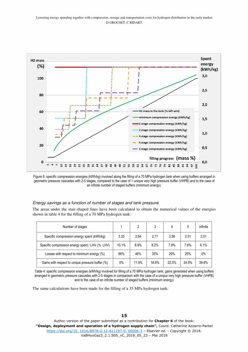
The effect of a pressure cascade on the energy needs is depicted in fig. 6 which presents the progressive
filling of a 70 MPa tank initially empty at �-/�E = )% (corresponding to a residual mass Y-/�E = :, C% in
the tank):
• With only 1 buffer at 90 MPa, or with all buffers at 90 MPa, according to eq.8, all hydrogen had
required a specific compression energy equal to 3.308 kWh/kg before being transferred to the tank
(red curve).
• If 2 staged buffers at 18 and 90 MPa are used, the first 22% of mass transferred to the tank comes
from the first buffer at 18 MPa and had only required a specific compression energy equal to 1.525
kWh/kg; while the following 72.2% comes from the second buffer at 90 MPa and had required
3.308 kWh/kg (blue curve).
• If 4 staged buffers are used, at 8, 18, 40.2 and 90 MPa, the first 7% transferred mass comes from
the first buffer at 8 MPa and had only required a specific compression energy equal to 0,967
kWh/kg; the following 15% transferred mass comes from the second buffer at 18 MPa and had
required an energy equal to 1.525 kWh/kg; the following 28% transferred mass comes from the
third buffer at 40.2 MPa and had required an energy equal to 2.236 kWh/kg; while the last 44.2%
comes from the fourth buffer at 90 MPa and had required 3.308 kWh/kg (orange curve).
• On this plot, the areas under the stair-shaped lines represent the energies spent for the compression
of the hydrogen to be transferred. Thus the area between the highest, red, straight line and the other
stair-shaped lines represent the energy saved thanks to the use of pressure cascades with 2, 3, 4 or 5
stages.
• On the opposite, the green curve shows the minimum compression energy which would be spent
with an infinite number of stages and buffers at increasing pressures equal to that of the tank. It is
also the energy that would be spent by a compressor connected to the tank and filling it directly.
The areas between the stair-shaped lines and that green curve represent the compression energiy
lost in the process of filling a tank by transfer from higher pressure buffers.
Lowering energy spending together with compression, storage and transportation costs for hydrogen distribution in the early market
D GROUSET, C RIDART
15 Author version of the paper submitted as a contribution for Chapter 6 of the book:
‘‘Design, deployment and operation of a hydrogen supply chain”, Coord. Catherine Azzarro-Pantel https://doi.org/10. 1016/B978-0-12-811197-0. 00006-3 – Elsevier ed. - Copyright © 2018.
VaBHyoGaz3_2.1.S05_vC_2018_05_23 – Mai 2018
Figure 6: specific compression energies (kWh/kg) involved along the filling of a 70 MPa hydrogen tank when using buffers arranged in geometric pressure cascades with 2-5 stages, compared to the case of 1 unique very high pressure buffer (VHPB) and to the case of
an infinite number of staged buffers (minimum energy).
Energy savings as a function of number of stages and tank pressure
The areas under the stair-shaped lines have been calculated to obtain the numerical values of the energies
shown in table 4 for the filling of a 70 MPa hydrogen tank:
Number of stages 1 2 3 4 5 infinite
Specific compression energy spent (kWh/kg) 3.33 2;94 2.71 2.58 2.51 2.01
Specific compression energy spent / LHV (% LHV) 10.1% 8.9% 8.2% 7.8% 7.6% 6.1%
Losses with respect to minimum energy (%) 66% 46% 35% 29% 25% 0%
Gains with respect to unique pressure buffer (%) 0% 11.9% 18.8% 22.5% 24.9% 39.8%
Table 4: specific compression energies (kWh/kg) involved for filling of a 70 MPa hydrogen tank, gains generated when using buffers arranged in geometric pressure cascades with 2-5 stages in comparison with the case of a unique very high pressure buffer (VHPB)
and to the case of an infinite number of staged buffers (minimum energy)
The same calculations have been made for the filling of a 35 MPa hydrogen tank:
Lowering energy spending together with compression, storage and transportation costs for hydrogen distribution in the early market
D GROUSET, C RIDART
16 Author version of the paper submitted as a contribution for Chapter 6 of the book:
‘‘Design, deployment and operation of a hydrogen supply chain”, Coord. Catherine Azzarro-Pantel https://doi.org/10. 1016/B978-0-12-811197-0. 00006-3 – Elsevier ed. - Copyright © 2018.
VaBHyoGaz3_2.1.S05_vC_2018_05_23 – Mai 2018
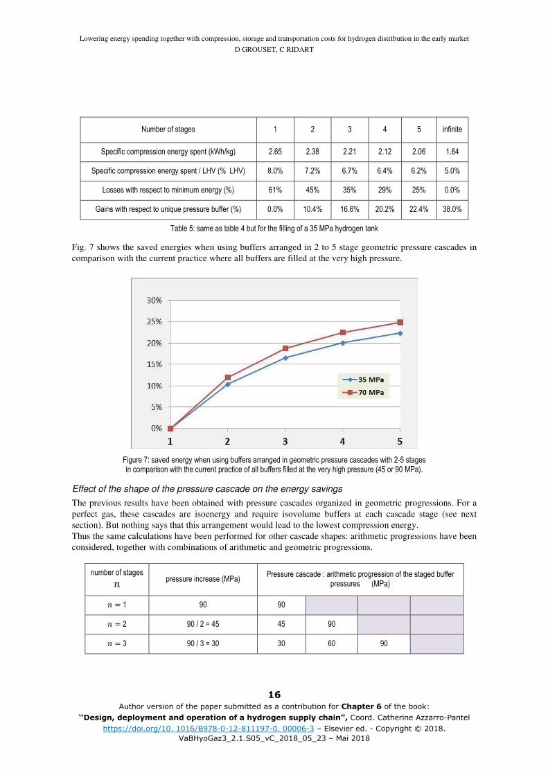
Number of stages 1 2 3 4 5 infinite
Specific compression energy spent (kWh/kg) 2.65 2.38 2.21 2.12 2.06 1.64
Specific compression energy spent / LHV (% LHV) 8.0% 7.2% 6.7% 6.4% 6.2% 5.0%
Losses with respect to minimum energy (%) 61% 45% 35% 29% 25% 0.0%
Gains with respect to unique pressure buffer (%) 0.0% 10.4% 16.6% 20.2% 22.4% 38.0%
Table 5: same as table 4 but for the filling of a 35 MPa hydrogen tank
Fig. 7 shows the saved energies when using buffers arranged in 2 to 5 stage geometric pressure cascades in
comparison with the current practice where all buffers are filled at the very high pressure.
Figure 7: saved energy when using buffers arranged in geometric pressure cascades with 2-5 stages in comparison with the current practice of all buffers filled at the very high pressure (45 or 90 MPa).
Effect of the shape of the pressure cascade on the energy savings
The previous results have been obtained with pressure cascades organized in geometric progressions. For a
perfect gas, these cascades are isoenergy and require isovolume buffers at each cascade stage (see next
section). But nothing says that this arrangement would lead to the lowest compression energy.
Thus the same calculations have been performed for other cascade shapes: arithmetic progressions have been
considered, together with combinations of arithmetic and geometric progressions.
number of stages R pressure increase (MPa)
Pressure cascade : arithmetic progression of the staged buffer pressures (MPa)
R = 1 90 90
R =2 90 / 2 = 45 45 90
R =3 90 / 3 = 30 30 60 90
Lowering energy spending together with compression, storage and transportation costs for hydrogen distribution in the early market
D GROUSET, C RIDART
17 Author version of the paper submitted as a contribution for Chapter 6 of the book:
‘‘Design, deployment and operation of a hydrogen supply chain”, Coord. Catherine Azzarro-Pantel https://doi.org/10. 1016/B978-0-12-811197-0. 00006-3 – Elsevier ed. - Copyright © 2018.
VaBHyoGaz3_2.1.S05_vC_2018_05_23 – Mai 2018
R = 4 90 / 4 = 22.5 22.5 45 67.5 90
Table 6: arithmetic progression staged buffer pressures as function of number of stages for a refueling at 70 MPa, (for a refueling at
35 MPa instead of 70 MPa, just divide the values of pressures by 2)
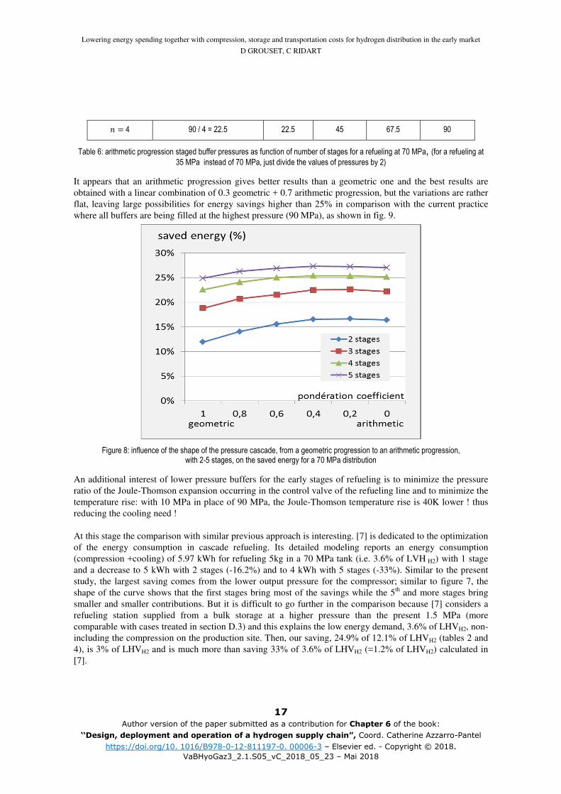
It appears that an arithmetic progression gives better results than a geometric one and the best results are
obtained with a linear combination of 0.3 geometric + 0.7 arithmetic progression, but the variations are rather
flat, leaving large possibilities for energy savings higher than 25% in comparison with the current practice
where all buffers are being filled at the highest pressure (90 MPa), as shown in fig. 9.
Figure 8: influence of the shape of the pressure cascade, from a geometric progression to an arithmetic progression, with 2-5 stages, on the saved energy for a 70 MPa distribution
An additional interest of lower pressure buffers for the early stages of refueling is to minimize the pressure
ratio of the Joule-Thomson expansion occurring in the control valve of the refueling line and to minimize the
temperature rise: with 10 MPa in place of 90 MPa, the Joule-Thomson temperature rise is 40K lower ! thus
reducing the cooling need !
At this stage the comparison with similar previous approach is interesting. [7] is dedicated to the optimization
of the energy consumption in cascade refueling. Its detailed modeling reports an energy consumption
(compression +cooling) of 5.97 kWh for refueling 5kg in a 70 MPa tank (i.e. 3.6% of LVH H2) with 1 stage
and a decrease to 5 kWh with 2 stages (-16.2%) and to 4 kWh with 5 stages (-33%). Similar to the present
study, the largest saving comes from the lower output pressure for the compressor; similar to figure 7, the
shape of the curve shows that the first stages bring most of the savings while the 5th and more stages bring
smaller and smaller contributions. But it is difficult to go further in the comparison because [7] considers a
refueling station supplied from a bulk storage at a higher pressure than the present 1.5 MPa (more
comparable with cases treated in section D.3) and this explains the low energy demand, 3.6% of LHVH2, non-
including the compression on the production site. Then, our saving, 24.9% of 12.1% of LHVH2 (tables 2 and
4), is 3% of LHVH2 and is much more than saving 33% of 3.6% of LHVH2 (=1.2% of LHVH2) calculated in
[7].

Lowering energy spending together with compression, storage and transportation costs for hydrogen distribution in the early market
D GROUSET, C RIDART
18 Author version of the paper submitted as a contribution for Chapter 6 of the book:
‘‘Design, deployment and operation of a hydrogen supply chain”, Coord. Catherine Azzarro-Pantel https://doi.org/10. 1016/B978-0-12-811197-0. 00006-3 – Elsevier ed. - Copyright © 2018.
VaBHyoGaz3_2.1.S05_vC_2018_05_23 – Mai 2018
3 Effect of pre-cooling on the compression energy
Considering eq.3 or eq.4, another possibility to decrease the compression work is to decrease �! by cooling
the hydrogen before compression. Calculations show that both the compression work and the compression
cooling energy decrease, respectively by -11 Wh/kg°C and -7 Wh/kg°C. Indeed, it is necessary to take also
into account the initial pre-cooling (+7.4 Wh/kg/°C) which cancels the gain of the final cooling. But globally,
with a COP of 3, an overall saving of 10.6 Wh/kg/°C can be reached. Thus 0.22 kWh/kg can be saved for a
cooling of 20°C at the entrance of the compressor, this is an extra 5% energy savings, as shown in table 7.
Compressor inlet temperature (°C) 20 0 -20 variation
Compressor electric consumption (kWélec) 11.03 10.30 9.57
Specific variation (Wh/kg°C) -11
Inter and final cooling needs (kWcool) 10.16 9.69 9.22
Specific variation (Wh/kg°C) -7,0
Initial cooling needs (kWcool) 0 0.53 1.06
Specific variation (Wh/kg°C) +7,4
Total electric power (kWélec) 14.42 13.71 12.99
Specific variation (Wh/kg°C) 10,6
Specific energy (kWh/kgH2) 4.33 4.11 3.90
Specific energy to LHV (% PCI) 13.1% 12.5% 11.8%
Energy saved (%) 0 5% 10%
Table 7: effect of hydrogen precooling on consumption for compression and cooling of 80 kg/day from a production pressure of 1.5 MPa to a buffer pressure of 90 MPa
Thus it is recommended to run the compressors with precooled hydrogen, at the lowest temperature possible,
according to the compressor requirements.
4 Necessary volume of the buffers
The delivering capacity of a refueling station at the peak hour mainly relies on the mass of hydrogen stored in
the HP buffers. Now, if the buffers are not all at the highest pressure, but are organized in a pressure cascade,
their volume has to be increased or else the peak hour performance will be reduced. Then the investment cost
of the staged buffers could be higher than that of smaller HP buffers. This section calculates the volume of
the necessary buffers and estimates their investment cost in order to compare overinvestment and energy
savings and to quantify the return on investment (ROI). But first the peak demand is defined.
Peak hour demand and buffer capacity

Lowering energy spending together with compression, storage and transportation costs for hydrogen distribution in the early market
D GROUSET, C RIDART
19 Author version of the paper submitted as a contribution for Chapter 6 of the book:
‘‘Design, deployment and operation of a hydrogen supply chain”, Coord. Catherine Azzarro-Pantel https://doi.org/10. 1016/B978-0-12-811197-0. 00006-3 – Elsevier ed. - Copyright © 2018.
VaBHyoGaz3_2.1.S05_vC_2018_05_23 – Mai 2018
The demand at a refueling station is not constant. It varies with the day and with the week. The result of a
statistical treatment of 385 U.S. refueling stations is presented in [13] from which data of figure 9a and 9b are
extracted and analyzed here:
• Friday is the busiest day in the week with a demand 7.5% above the average, while Monday is the
quietest day.
• 3 pm is the busiest hour in the day with, on Friday, 7.8% of the total of the day, or 1.87 times the
average of the day.
• 7 am and 7 pm are on the Friday daily average while the 12h period in between is above the
average; thus it appears there is no peak hour but a large peak period.
• The area above the average line represents 27.5% of the total area.
Figure 9: hourly (A) and daily (B) average gasoline distribution profile (data are from [13])
The minimum capacity for the HRS compressor would correspond to the average flowrate, with a 24h/day
operation. Then it will be necessary the buffer contains an extra mass of hydrogen deliverable at the desired
pressure equal to 27.5% of the daily dispensed hydrogen. During the period 7 am to 7 pm, destocking
hydrogen will occur from the buffer and its pressure will decrease down to the minimum acceptable pressure;
after 7 pm, the hydrogen dispensed to the vehicle tanks is less than the average and the compressor delivers
more than what is dispensed to the vehicles, thus stocking in the buffer will occur and its pressure will
increase; the compressor will refill the buffer at its nominal pressure until 7 am, with an extra mass equal to
27.5% of the daily hydrogen dispensed.
In fact, it is recommended to oversize the compressor to be able to cope with some extra affluence, invisible
in the average statistics. With a higher capacity compressor the buffer will sooner recover its nominal
pressure and then the compressor will stop, so that it will operate less than 24h/day.
Also, when dealing with small capacity HRS, dedicated to small captive fleets, the refueling behavior may be
different and the delivery profile of the station has to be defined carefully in order to adjust the peak hour
performance.
The following calculations consider a compressor oversized by a factor of 2 and a mass of hydrogen that can
be dispensed at the nominal delivery pressure during the peak hour or period, ���/E, equal to 25% of its
daily capacity (i.e. ���/E = 20 kg for an 80 kg/day HRS). Thus the compressor only runs 12h/day in
average and with such a value of ���/E, it is possible to face 3 hours of peak demand at 8% of the daily
average without the help of the compressor. With the help of the compressor, capable of delivering 8.33% of

Lowering energy spending together with compression, storage and transportation costs for hydrogen distribution in the early market
D GROUSET, C RIDART
20 Author version of the paper submitted as a contribution for Chapter 6 of the book:
‘‘Design, deployment and operation of a hydrogen supply chain”, Coord. Catherine Azzarro-Pantel https://doi.org/10. 1016/B978-0-12-811197-0. 00006-3 – Elsevier ed. - Copyright © 2018.
VaBHyoGaz3_2.1.S05_vC_2018_05_23 – Mai 2018
the daily capacity per hour, the buffer will have recovered its nominal pressure at the end of the most
demanding hour. In fact, the maximum capacity of the refueling station is twice its nominal capacity and the
vehicle fleet can increase by a factor of 2 before the station is overwhelmed.
Analytical formulation of buffer volumes
The mass of hydrogen ���/E that can be delivered at the nominal pressure (35 or 70 MPa) is now defined
and this mass corresponds to a volume ���/E
���/E = ���/E �&%,-/�E$ ��. %!�Tanks of volume ���/E have to be refilled from �-/�E,! to �-/�E,� with ���/E while the buffer pressure
decreases from �O���,! to �-/�E,�. Beside "�, the tank filling pressure ratio, a new pressure ratio is
introduced, Z�, the overpressure of the initial full buffer with respect to the objective full tank pressure:
"� = �-/�E,� �-/�E,!$ = � �-/�E$ ��. %��Z� = �O���,! �-/�E,�$ ��. %%�
Considering the mass conservation during the balancing of pressures between buffer and tanks and a perfect
gas, the volume of the buffer �O��� necessary to fill the volume ���/E in a pressure ratio "�, with a buffer
overpressure Z� can be calculated as: �O��� ���/E[ = "� − �� ["� ∗ Z� − ��][ ��. %2�It should be noted when writing eq.17, that the balancing of pressure is supposed to be isothermal, whereas
compression occurs in the tank and heats hydrogen and expansion occurs in the buffer… Thus eq.17 is only
valid after tank and buffer have recovered their initial temperature...
Now, the flow of hydrogen is not conducted until the exact isothermal balancing of pressure because it would
be long. In fact, taking into account the temperature rise in the tank during the refueling, it is necessary to fill
the tank with an overpressure so that, after the tank has cooled down to ambient temperature, the pressure has
decreased to the desired �-/�E,�. Thus it is considered that the tanks must be refilled while the buffer pressure decreases to �O���,�,�+�,
keeping a minimum overpressure �,�+�:
�O���,�,�+� �-/�E,�$ = �,�+���. %)�Then, the volume of the necessary buffer is calculated as: �O��� ���/E[ = "� − �� ["� ∗ Z� − �,�+��][ ��. %:�Moreover, hydrogen is not a perfect gas and a correction has to be introduced as a ratio of compressibility
factors:
�O��� ���/E[ = ^ �O���,! �-/�E,�[ _ ∗ "� − �� ["� ∗ Z� − �,�+��][ ��. %;�Finally, eq.26 allows to estimate easily the volume of the necessary buffer for the peak hour demand, without
detailed modeling of the unsteady filling of the tank including hydrogen heating and heat transfer to the tank
walls, as done in [7], [8]. In fact, all the thermal behavior of hydrogen and tank is represented by the factor

Lowering energy spending together with compression, storage and transportation costs for hydrogen distribution in the early market
D GROUSET, C RIDART
21 Author version of the paper submitted as a contribution for Chapter 6 of the book:
‘‘Design, deployment and operation of a hydrogen supply chain”, Coord. Catherine Azzarro-Pantel https://doi.org/10. 1016/B978-0-12-811197-0. 00006-3 – Elsevier ed. - Copyright © 2018.
VaBHyoGaz3_2.1.S05_vC_2018_05_23 – Mai 2018
�,�+�. According to the SAE-J2601 standard [4], to compensate the heating of the hydrogen and tank, it is
possible to overfill the tank (over its nominal pressure), so that after the natural cooling, its pressure
decreases to its nominal pressure. Target pressures with a 1.10 overpressure factor are current when fueling at
high ambient temperature (e.g. a target of 77 MPa for the refueling end for a nominal 70 MPa after natural
cooling). Thus using a �,�+�=1.1 in eq.26 assumes that the pressure can increase by a factor 1.1 in the tank,
due to the hydrogen temperature increase in the same ratio: an increase from 290 to 320 K, which is rather
low and would mean that hydrogen has been cooled before entering the tank. Without precooling, hydrogen
temperature would be higher (but under 85°C), and either �,�+� should be chosen higher than 1.10 to keep
good peak hour performance, or the flow rate should be decreased in order to decrease hydrogen temperature.
Thus as long as �,�+� is correctly estimated there is no necessity of detailed thermal modeling, nor to
consider filling rate, tank filling duration, time between two successive vehicles…
Now, to estimate correctly �,�+�, information can be gained from detailed transient heat transfer modeling
inside the tank and ref. [15] to [20] will be useful, especially [15] and [16] for the model description and [17]
for results concerning the temperature raise as functions of filling rate, initial tank pressure and ambient
temperature.
Buffer volume with only 1 very high pressure buffer (VHPB) at the highest pressure 45 MPa or 90
MPa (reference case)
For an 80 kg/day refueling station, ���/E =20 kg;
with �&%,-/�E =24kg/m3 at 35MPa or 40.24kg/m3 at 70MPa,
���/E is obtained: ���/E,2:#?/ =0.833m3 and ���/E,=!#?/ =0.497m3.
"� = %: for � = )%
and Z� = �, %C:for �O���,!=90MPa and �-/�E,�=70MPa or for �O���,!=45MPa and �-/�E,�=35MPa,
Thus following eq.26: �O��� ���/E[ =5.48 and finally: �O���,):#?/ = ). :;�2, �O���,H!#?/ = %. =%�2.
Buffer volumes with staged pressure
In the case of staged pressure buffers, the approach is formally the same and the only difference in the
formulas is the substitution of the overall large pressure ratio "� by the smaller pressure ratio .� of each
stage.
If the buffer pressures are staged in a geometric progression, all .� are equal and then the buffer volumes are
equal at each stage; the volumes are given in table 8. It is clear that each stage requires a smaller volume of
buffer, but globally, the total volume of buffers is larger.
number of stages R stage pressure ratio
.�
�O��� ���/E[
for each stage R = 1 .� = "� =25 5.48
R =2 .� = (25)1/2 = 5.0 4.57

Lowering energy spending together with compression, storage and transportation costs for hydrogen distribution in the early market
D GROUSET, C RIDART
22 Author version of the paper submitted as a contribution for Chapter 6 of the book:
‘‘Design, deployment and operation of a hydrogen supply chain”, Coord. Catherine Azzarro-Pantel https://doi.org/10. 1016/B978-0-12-811197-0. 00006-3 – Elsevier ed. - Copyright © 2018.
VaBHyoGaz3_2.1.S05_vC_2018_05_23 – Mai 2018
R =3 .� = (25)1/3 = 2.92 3.76
R = 4 .� = (25)1/4 = 2.236 3.16
R = 5 .� = (25)1/5 = 1.903 2.71
Table 8: volume of necessary buffers in case of geometric progression staged buffer pressures
5 Cost of the storage buffers
If all buffers are designed for the highest pressure, as in [7] or [8], the investment cost of the buffers will be
higher. But as the lower pressure buffers will never experience the highest pressure, they can be designed for
lower pressure; the overinvestment could be small.
Yet, composite bottles are only available for a few capacities and a few nominal pressures. Then the
commercial available nominal pressures do not respect a geometrical progression (but they could lead to
better energy savings as shown in fig. 6). Adequate staged volumes have to be calculated in function of each
pressure ratio according to eq.20; they do not have equal values and furthermore will not correspond to the
commercial available volumes: then some buffers will have to be oversized, inducing additional cost.
It is considered here that bottles are available only with a unit volume of 300 L and for nominal pressures of
10, 20, 30, 52.5 and 90 MPa. The number of necessary 300L bottles is calculated in table 9 for each stage of
the storage of an 80kg/day 70 MPa refueling station. The cost of the storage is then obtained, using eq.10.
The saving percentage is obtained from figure 8.
Number of stages 1 2 3 4 5
10 MPa buffer number
3
20 MPa buffer number
4 3
30 MPa buffer number
6 5 3 3
52.5 MPa buffer number
3 3 3
90 MPa buffer number 6 4 3 3 3
Storage cost (k€) 63.0 66.1 72.6 75.5 76.8
Annual energy savings (%) reference 16.0% 22.4% 25.2% 26.3%
Annual energy savings (k€) reference 1.52 2.13 2.40 2.51
Return on investment (years) reference 2.0 4.5 5.2 5.5
Table 9: effect of number of stages on number of bottles of 300 L needed at each stage, cost of storage, energy savings and return on investment for an 80 kg/day 70 MPa HRS
It can be seen that:

Lowering energy spending together with compression, storage and transportation costs for hydrogen distribution in the early market
D GROUSET, C RIDART
23 Author version of the paper submitted as a contribution for Chapter 6 of the book:
‘‘Design, deployment and operation of a hydrogen supply chain”, Coord. Catherine Azzarro-Pantel https://doi.org/10. 1016/B978-0-12-811197-0. 00006-3 – Elsevier ed. - Copyright © 2018.
VaBHyoGaz3_2.1.S05_vC_2018_05_23 – Mai 2018
• In the reference case of current practice, with one only very high pressure stage (90 MPa), 6 bottles
of 300L would be needed (exact theoretical total volume needed is 1816L) for a total cost of 63k€;
the annual operation reference cost of energy is 9.53k€/year, according to table 2.
• With 2 stages, when introducing an intermediate 30 MPa stage, 4 300L 90 MPa bottles would be
enough (theoretical volume needed is 1263L) together with 6 300L 30 MPa bottles (theoretical
volume needed 1663L); the total cost is 66.1k€ and the energy saving is 16% with respect to the
reference case; thus the return on investment is only 2 years.
• With 4 stages, introducing intermediate stages at 14.5 MPa, 30 MPa and 52.5 MPa, 3 300L 90 MPa
bottles would be used, (even if too large: theoretical volume needed is 793L) together with 3 300L
52.5 MPa bottles (theoretical volume 809L), 3 300L 30 MPa bottles (theoretical volume 979L) and
4 300L 20 MPa bottles (theoretical volume 1479L); the total cost is 75.5k€ and the energy saving is
25.2%, thus the return on investment is 5.2 years.
• The use of staged pressure buffers increases the total storage volume and the investment cost. The
overinvestment payback time increases with the number of stages, but remains acceptable.
6 Conclusion for hydrogen distribution on the production site
Compressing hydrogen is inevitable when fuel cell cars have to be refueled at high pressure. The energy cost
of compressing and cooling hydrogen is high. In the case of hydrogen dispensed on the production site, it can
reach 3.50 or 4.4 kWh per kg of hydrogen transferred to the car tank at 35 or 70 MPa, in a reference case
corresponding to best current practice. Recommendations have been made in order to avoid spending even
higher energy, which is current in small refueling stations.
The study shows that this energy need can be reduced by 22%, 25% or even 27% when judiciously using 3,
4 or 5 stages of buffers organized in a pressure cascade for the filling of the tank. Whereas the total volume
of the staged pressure buffers is higher than the volume of an only very high pressure buffer, the extra cost is
acceptable and the energy saving results in an acceptable payback time for the overinvestment: 4.5 to 5.5
years.
Precooling the hydrogen before the compression would also lead to energy savings: an extra 5 to 10% can
be gained, and compressor technology could be improved to admit cooled hydrogen.
D - Case of a production unit supplying several distant refueling stations
Currently, most of the hydrogen dispensed is supplied from large and distant production units: only few
HRSs have an onsite production.
Hydrogen is usually supplied in steel bottle bundles or trailer tubes, trucked to the station. These steel
containers have a low specific content, a bundle of 12 steel 50L 20 MPa bottles weighing 1010kg for a
content of 9kg H2 only, or a pay load of only 0.9%! A trailer with 14 steel 1535L 20 MPa tubes weights 31t
for a content of 320kg H2: a 1.04% pay load!
Transportation energy costs are high as distances between production units and refueling stations can be long
and the tractor and its trailer are heavy and greedy: a 38t hauler can need 35L of diesel fuel per 100 km.
Then, for 320 kgH2 of a tube trailer, with 9.85 kWh/LDiesel, and 0.270 kgCO2/kWhDiesel, it is 2.15 kWh/kgH2,
6.5% of LHVH2 and 0.6 tCO2/tH2 for each 100 km of distance between production and distribution! And even
much more for bottle bundles!

Lowering energy spending together with compression, storage and transportation costs for hydrogen distribution in the early market
D GROUSET, C RIDART
24 Author version of the paper submitted as a contribution for Chapter 6 of the book:
‘‘Design, deployment and operation of a hydrogen supply chain”, Coord. Catherine Azzarro-Pantel https://doi.org/10. 1016/B978-0-12-811197-0. 00006-3 – Elsevier ed. - Copyright © 2018.
VaBHyoGaz3_2.1.S05_vC_2018_05_23 – Mai 2018
1. Potential for reducing energy demand
When the production unit supplies hydrogen to several distant refueling stations, energy for transportation by
truck and for re-compression on the distribution site must be considered, but the distribution unit works in the
same way as when on the production site (figure 2). Potentials explored in this paper to lower the energy
spending of actual or near future small refueling stations are:
- reduce the distances between production unit and distribution sites to a 50 km average.
- use small transportable containers of high pressure light composite bottles: 30 or 50 MPa or even
more, when available….
- use these transportable containers in place of intermediate pressure buffers on the distribution site
(figure 10).
Figure 10: schematic view of the equipment for filling the HP tank of a hydrogen vehicle in a refueling station supplied by truck from a distant hydrogen production unit
Distributed hydrogen production to reduce transportation distances
Reducing the hydrogen transportation distances to about 50 km (always less than 100 km) is a specific
possible advantage of distributed hydrogen production, promoted by the VABHYOGAZ3 project which
considers hydrogen production from biogas. As biogas can be produced from many kinds of waste and in lots
of places, hydrogen refueling stations will never be far from a hydrogen source. This is also the case for
hydrogen production from electrolyser. In the contrary, it is not the case for the current practice as hydrogen
is by now mainly produced by steam reforming in large units located, for example, on refinery sites and
hydrogen transportation distances can then be very long, sometimes more than 500 km, inducing 10 times
more energy spent and CO2 emissions for transportation!
Small high pressure light composite bottle transportable containers
The use of high pressure composite bottle containers for hydrogen transportation, in order to reduce
transportation cost and energy has been suggested for a long time: Nexant report [10] from 2008 considers
7000 psi (48 MPa) trailers with a capacity of 1000 kg H2; as does NREL report [9] from 2012 which
considers a tube trailer at 35 MPa with a capacity of about 800 kg. Commercial offers can be obtained for
containers at 25 or 30 MPa (as reported in section B.2), but these containers are currently only used for
natural gas transportation. European Commission programs promoted developments in this field, but only a
few prototypes have been realized and the current practices are still 20 MPa steel tube trailers with a capacity
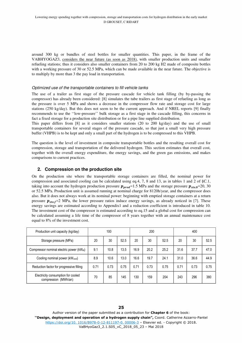
Lowering energy spending together with compression, storage and transportation costs for hydrogen distribution in the early market
D GROUSET, C RIDART
25 Author version of the paper submitted as a contribution for Chapter 6 of the book:
‘‘Design, deployment and operation of a hydrogen supply chain”, Coord. Catherine Azzarro-Pantel https://doi.org/10. 1016/B978-0-12-811197-0. 00006-3 – Elsevier ed. - Copyright © 2018.
VaBHyoGaz3_2.1.S05_vC_2018_05_23 – Mai 2018
around 300 kg or bundles of steel bottles for smaller quantities. This paper, in the frame of the
VABHYOGAZ3, considers the near future (as soon as 2018), with smaller production units and smaller
refueling stations; thus it considers also smaller containers from 20 to 200 kg H2 made of composite bottles
with a working pressure of 30 or 52.5 MPa, which can be made available in the near future. The objective is
to multiply by more than 3 the pay load in transportation.
Optimized use of the transportable containers to fill vehicle tanks
The use of a trailer as first stage of the pressure cascade for vehicle tank filling (by by-passing the
compressor) has already been considered: [8] simulates the tube trailers as first stage of refueling as long as
the pressure is over 5 MPa and shows a decrease in the compressor flow rate and storage cost for large
stations (250 kg/day). But this does not seem to be the current approach. And if NREL reports [9] finally
recommends to use the ‘‘low-pressure’’ bulk storage as a first stage in the cascade filling, this concerns in
fact a fixed storage for a production site distribution or for a pipe line supplied distribution.
This paper differs from [8] as it considers smaller stations (20 to 200 kg/day) and the use of small
transportable containers for several stages of the pressure cascade, so that just a small very high pressure
buffer (VHPB) is to be kept and only a small part of the hydrogen is to be compressed to this VHPB.
The question is the level of investment in composite transportable bottles and the resulting overall cost for
compression, storage and transportation of the delivered hydrogen. This section estimates that overall cost,
together with the overall energy expenditure, the energy savings, and the green gas emissions, and makes
comparisons to current practices.
2. Compression on the production site
On the production site where the transportable storage containers are filled, the nominal power for
compression and associated cooling can be calculated using eq.4, 7, 8 and 13, as in tables 1 and 2 of §C.1,
taking into account the hydrogen production pressure ��.,�=1.5 MPa and the storage pressure �-,,!=20, 30
or 52.5 MPa. Production unit is assumed running at nominal charge for 8120h/year, and the compressor does
also. But it does not always work at its nominal power: beginning with emptied storage containers at a return
pressure �-,,�=2 MPa, the lower pressure ratios induce energy savings, as already noticed in [7]. These
energy savings are estimated according to Appendix1 and a reduction coefficient is introduced in table 10.
The investment cost of the compressor is estimated according to eq.15 and a global cost for compression can
be calculated assuming a life time of the compressor of 8 years together with an annual maintenance cost
equal to 8% of the investment cost.
Production unit capacity (kg/day) 100 200 400
Storage pressure (MPa) 20 30 52.5 20 30 52.5 20 30 52.5
Compressor nominal electric power (kWél) 9.1 10.8 13.5 16.9 20.2 25.2 31.6 37.7 47.0
Cooling nominal power (kWcool) 8.9 10.6 13.0 16.6 19.7 24.1 31.0 36.6 44.9
Reduction factor for progressive filling 0.71 0.73 0.75 0.71 0.73 0.75 0.71 0.73 0.75
Electricity consumption for cooled compression (MWh/an)
70 85 145 130 159 204 243 296 380

Lowering energy spending together with compression, storage and transportation costs for hydrogen distribution in the early market
D GROUSET, C RIDART
26 Author version of the paper submitted as a contribution for Chapter 6 of the book:
‘‘Design, deployment and operation of a hydrogen supply chain”, Coord. Catherine Azzarro-Pantel https://doi.org/10. 1016/B978-0-12-811197-0. 00006-3 – Elsevier ed. - Copyright © 2018.
VaBHyoGaz3_2.1.S05_vC_2018_05_23 – Mai 2018
Electricity cost (k€/an) 5.6 6.8 8,7 10.4 12.7 16.3 19.4 23.7 30.4
Specific consumption for cooled compression (kWh/kgH2)
1.91 2.33 2.99 1.78 2.18 2.79 1.66 2.03 2.60
Specific consumption for cooled compression (% PCI)
5.7% 7.0% 9.0% 5.3% 6.5% 8.4% 5.0% 6.1% 7,8%
Compressor investment cost (k€) 140 146 155 173 180 190 213 222 235
Global cost for compression and cooling (€/kg H2)
0.90 0.96 1,05 0.59 0.64 0,70 0.40 0.43 0,49
Table 10: energy spent and compression cost for cooled compression on production site, as function of the production unit capacity and of the transportable storage pressure (hydrogen production pressure 1.5 MPa, initial storage pressure 2 MPa)
Compression on the production site benefits of the scale effect: the higher the flow rate, the better the
efficiency of the compressor and the lower the specific investment cost of it. Thus the compression specific
cost for hydrogen decreases significantly when increasing the production unit size: -55% for 400 kg/day with
respect to 100 kg/day.
3. Compression on the distribution site
On the distribution site, a compressor power can be calculated if all the daily distributed hydrogen is assumed
to be recompressed from the transportable storage pressure �-,,!=20, 30 or 52.5 MPa to the high pressure
buffers at �O���=45 or 90 MPa, as usual in current practices [8].
Again, the compressor will start at lower pressure ratios, which induces energy savings estimated according
to Appendix2 and a reduction coefficient is applied to the electric energy demand.
Moreover, the use of the transportable containers as first stages for direct filling of the vehicle tank will
reduce the quantity of hydrogen to be compressed to the higher buffer pressure. Thus the nominal flow rate
of the compressor is reduced by a ‘‘by-pass coefficient’’ (with respect to the daily distribution capacity) to be
estimated as a function of the utilization strategy of the transportable containers, detailed in the following
sections.
Table 11 gives the reference values in the current practices, namely storage pressure of 20 MPa, with the first
reduction factor, but without the second: no by-pass of the compressor is considered.
Refueling station capacity (kg/day) 20 80 200
Buffer pressure (MPa) 45 90 45 90 45 90
Compressor nominal electric power (kWel) 4.75 6.25 16.5 21.8 37.7 49.6
Cooling nominal power (kWcool) 4.58 5.85 15.9 20.2 36.1 45.6
Reduction factor for progressive emptying 0,50 0.59 0,50 0.59 0,50 0.59
Electric consumption for cooled compression (MWh/an) 13,7 21.2 48 74 109 168
Electricity cost (k€/an) 1,1 1.7 3,8 5.9 8,7 13.4

Lowering energy spending together with compression, storage and transportation costs for hydrogen distribution in the early market
D GROUSET, C RIDART
27 Author version of the paper submitted as a contribution for Chapter 6 of the book:
‘‘Design, deployment and operation of a hydrogen supply chain”, Coord. Catherine Azzarro-Pantel https://doi.org/10. 1016/B978-0-12-811197-0. 00006-3 – Elsevier ed. - Copyright © 2018.
VaBHyoGaz3_2.1.S05_vC_2018_05_23 – Mai 2018
Specific consumption for cooled compression (kWh/kgH2) 1.88 2.9 1.63 2.52 1.49 2.30
Specific consumption for cooled compression (% LHV) 5.6% 8.7% 4.9% 7.5% 4.45 6.87
Compressor investment cost (k€) 104 111 157 168 207 222
Global cost for compression and cooling (€/kg H2) 3.07 3.36 1.24 1.39 0.70 0.81
Table 11: reference values for current practices: energy spent for cooled compression on the distribution site, for initial storage pressure of 20 MPa, final storage pressure 2MPa and compression of all the hydrogen to the buffer pressure,
It can be seen that for the small HRS, with the current practice the cost of compression can be very high,
higher that the cost of compression in the production unit, even if the compressor power is lower.
Next sections discuss how improved container utilization scenarios can lower compressor investment cost
and energy demand when using 30 MPa and 52.5 MPa storage containers.
4. Scenarios for transportable container utilization
The idea is to place several transportable containers on the distribution site and to use them, as much as they
are, as first stages for filling tank vehicles, while the compressor takes hydrogen in the lowest pressure
container, compresses it and fills a higher pressure buffer. This unique buffer allows completing the filling of
the vehicle tank to its nominal pressure.
In the case in which the transportable containers have a nominal pressure higher than the vehicle tank
nominal pressure (i.e. �-, =52.5 MPa for �-/�E =35 MPa), the compressor in no longer necessary, nor is the
highest pressure buffer. This case results in a drastic simplification of the refueling station with an investment
considerably reduced and an energy consumption also drastically reduced. This case is considered first.
Refueling at �-/�E=35 MPa with storage containers at �-, = 52.5 MPa
With storage at a higher pressure than the tank to fill, the compressor is of no use, but it is necessary to
dispose of several storage containers on the distribution site, and these containers will have to be returned to
the production unit with a non-negligible residual hydrogen pressure.
An analytical formulation has been developed to calculate this residual pressure and it is presented in
Appendix3. The result depends on the number of storage containers present on the distribution site. It is easy
to understand that with only one available storage container, this one will not be able to ensure a complete 35
MPa tank filling as soon as its pressure is lower than 35 MPa, or even lower than 38.5 MPa to take into
account the heating of hydrogen during filling (�,�+� =1,10). Thus it should be substituted by another one
and returned to the production unit with a residual pressure �-,,�,�=38.5 MPa, i.e. �-,,�=73.3%. With a
second storage available, this first one can be further used as a first stage for tank filling and its residual
hydrogen pressure will then depend on the filling state of the vehicle tanks �-/�E.
The results are given on the table 12 as a function of the number of containers on the distribution site, which
is the number of stages in the refueling, for �-/�E =5% (�-/�E,!=1.75 MPa). Table 12 also gives the
contribution of each stage to refueling (percentage of tank filling). In the case in which the average �-/�E
would be higher, the values of �-,,� would be higher.
Number of storages
�
Stage � �-,,�,�∆�-/�E,�
Stage � − � �-,,�,%∆�-/�E,%
Stage � − % �-,,�,2∆�-/�E,2�
Stage � − 2 �-,,�,)∆�-/�E,)
Residual fraction returned to production �-,,�

Lowering energy spending together with compression, storage and transportation costs for hydrogen distribution in the early market
D GROUSET, C RIDART
28 Author version of the paper submitted as a contribution for Chapter 6 of the book:
‘‘Design, deployment and operation of a hydrogen supply chain”, Coord. Catherine Azzarro-Pantel https://doi.org/10. 1016/B978-0-12-811197-0. 00006-3 – Elsevier ed. - Copyright © 2018.
VaBHyoGaz3_2.1.S05_vC_2018_05_23 – Mai 2018
1 38.5 MPa
95% 73.3%
2 38.5 MPa
43.3% 21.8 MPa
51.7% 41.5 %
3 38.5 MPa
33.9% 25.4 MPa
31.6% 13.3 MPa
29.5% 25.3 %
4 38,5 MPa
30.4% 26.7 MPa
25.5% 17.0 MPa
21.3% 8.8 MPa 17.8%
16.7 %
Table 12: Effect of the number of available 52.5 MPa storage containers: contribution of each stage to the refueling at �-/�E=35 MPa,
starting with �-/�E=5%; residual pressure for each stage and residual fraction returned to the production unit
Even with 4 stages, the residue returned to the production unit is high, �-,,)=16.7%; but the advantages are:
100% of energy mentioned in table 12 saved and compressor and buffer investment costs also saved.
Refueling at �-/�E=35 MPa with storage containers at �-,=30 MPa
With storage containers at �-,=30 MPa it is necessary to use a compressor which will increase the pressure
of a fraction of the hydrogen to fill a buffer at �O���=45 MPa. The analytical equations to calculate this
fraction, together with the energy saving, have been formulated and are presented in Appendix4. The results
depend again on the filling state of the vehicle tanks, �-/�E=5%; but the residual hydrogen pressure with
which the containers are returned to the production unit can now be chosen and here �-,,�,�=6.67% or �-,,�,�=2 MPa.
On table 13 column 2, the fraction of hydrogen to be compressed is shown (on a total of � − �-/�E�=95%)
and this number allows sizing a smaller compressor for the distribution unit; its capacity can be reduced by a
factor of 2.5 - 3 with 3 or 4 stages. The columns 3, 4 and 5 give the contributions of the previous stages to the
refueling and the pressure at which the storage container is shifted to the lower stage. The last column gives
the reduction factor of the energy demand, with respect to the reference case in which 20 MPa storage
containers would be completely transferred to the high pressure buffer. It can be noticed that even with 1
available storage container only, it is possible to organize a direct connection for a prefilling of the tank
before completing the refueling from the buffer.
Number of storages
�
Stage � (compressor) �-,,�,�∆�-/�E,�
Stage � − � �-,,�,%∆�-/�E,%
Stage � − % �-,,�,2∆�-/�E,2�
Stage � − 2 �-,,�,)∆�-/�E,)
Energy demand reduction with respect
to reference case
1 2 MPa 75 %
2 MPa 20 %
0.75
2 2 MPa 53,7%
17,8 MPa 41,3 %
0.591
3 2MPa 40,3%
23,3 MPa 23,7 %
13,9 MPa 31,0 %
0.480
4 2MPa 34%
25,4 MPa 15,6 %
19,4 MPa 20,4 %
11,5 MPa 24,9%
0.359
Table 13: Effect of the number of available 30 MPa storage containers; stage R is connected to the compressor; �-,,�,�=2 MPa;
contribution of each stage to the refueling at �-/�E=35 MPa, starting with �-/�E=5%; residual pressure for each stage and reduction
factor for the compressor energy demand
Lowering energy spending together with compression, storage and transportation costs for hydrogen distribution in the early market
D GROUSET, C RIDART
29 Author version of the paper submitted as a contribution for Chapter 6 of the book:
‘‘Design, deployment and operation of a hydrogen supply chain”, Coord. Catherine Azzarro-Pantel https://doi.org/10. 1016/B978-0-12-811197-0. 00006-3 – Elsevier ed. - Copyright © 2018.
VaBHyoGaz3_2.1.S05_vC_2018_05_23 – Mai 2018
Other calculations have been made for �-/�E=70 MPa and �-,=52.5 and 30 MPa. Because of the greater
difference between tank and storage pressures, the contribution of the compressor is higher and the energy
saving lower. But the compressor capacity can still be reduced by a factor of 1.5-2.5.
5. Detailed characteristics and costs for 20 kg/day distribution units
An example is detailed, named P_100_D_20, it considers 5 small distribution units of 20 kg/day within a
distance of 50 km of their supplying production unit. The technical details and costs are analyzed and
compared in 3 cases in table 14:
a) steel 20 MPa storage, 1 stage, no compressor by-pass (reference case)
b) 4 stages 30 MPa composite storage;
c) 4 stages 52.5 MPa composite storage.
Cooled compression
It appears that for a distribution at 35 MPa, the global costs for cooled compression is reduced by 28% and
spent energy and CO2 emissions are reduced by 55% in case b (30 MPa storage containers) compared to case
a (20 MPa reference). They are reduced to 0 in case c (52.5 MPa storage containers). In case b, the nominal
power of the compressor is much lower as a large fraction of hydrogen can by-pass it and so are the
consumption and CO2 emissions (green-house gas emissive power of French electricity is taken at 60
gCO2/kWhel). Nevertheless, for so small distribution units, the cooled compression cost is high: between 2.2
and 3.36 €/kg. Having no compression on the distribution site is a very large advantage.
High pressure buffer
Using higher pressure storage containers induces also a benefic effect on the necessary volume for high
pressure buffers in the distribution station. But this cost remains low: between 0 and 0.26 €/kg.
Transportable storage containers
Even if the transportable storage containers might rather be used on a rental basis, investment costs and
specific costs are estimated (costs without margin). The calculations have shown that the best is having
storage units with a capacity of about 1 day of distribution (thus here 20kg).
a) in the current practice, 20 MPa storage containers consist in bundles with 12 50L steel bottles for an
overall mass of 1010 kg (0.9% of hydrogen content only).
b) 30 MPa composite storage containers would be made from 2 bottles of 350L containing 14.7 kg H2
for a mass of 480 kg (3.2% hydrogen content).
c) 52.5 MPa composite storage containers will be made from 2 bottles of 300L containing 19.8 kg H2
for a mass of 660 kg (3.0% hydrogen content).
These scenarios take the following into account:
• �-,, the residual hydrogen returned to the production unit when storage considered as empty,
• a minimum net autonomy of 2 days on the distribution site,
• a container number at least equal to the stage number (4 for cases b and c),
• a rotation each 2 or 3 days for the delivery of the bundles or containers,
• at least 1 container left on the production site for being filled.
This gives the total minimum number of containers, the overall autonomy and the investment cost for the
storage. The autonomy is then between 6.1 and 8.6 days. The absence of compressor induces a high residual
pressure in the returned containers and increases of 1 unit the number of necessary containers for 35 MPa
distribution. With 52.5 MPa storage containers, due to the larger H2 mass of containers, the autonomy of the
stations exceeds 3 days. Thanks to their long life time, the depreciation of storage container investment cost

Lowering energy spending together with compression, storage and transportation costs for hydrogen distribution in the early market
D GROUSET, C RIDART
30 Author version of the paper submitted as a contribution for Chapter 6 of the book:
‘‘Design, deployment and operation of a hydrogen supply chain”, Coord. Catherine Azzarro-Pantel https://doi.org/10. 1016/B978-0-12-811197-0. 00006-3 – Elsevier ed. - Copyright © 2018.
VaBHyoGaz3_2.1.S05_vC_2018_05_23 – Mai 2018
is taken over 20 years, together with a 1.5% annual maintenance cost. Finally, the specific storage cost
remains high: from 0.63 to 1.86 €/kg, but the increase for cases b and c with respect to case a is lower than
the savings on the specific compression cost.
Transportation material
The transportation material consists in a tractor and a flatbed trailer equipped with a handling crane, the
calculation model shows:
a) 5 bundles have to be delivered every 2 days to each of the 5 stations; the total mass is more than 25
tons and would necessitate a 38t tractor and trailer with a high investment and a specific cost of
0.55 €/kg (including maintenance cost).
b) 3 containers have to be each 2 days to each HRS: the load is only 7.2t and will require lighter
tractor and trailer, with an specific cost divided by 2: 0.26 €/kg
c) the station autonomy is larger than 3 days and the supplying of 2 or 3 stations every 3 days is
planned, with the same material as for b.The storage trailer load will be 8t for 35 MPa distribution
or 6t for 70 MPa and the specific cost of the same order.
The round delivery trip for 3 or 5 stations is 6 or 9 hours long for 200 or 300 km as the distance between
stations is assumed 50 km, with 30 min for unloading / loading in each place. Total mileage is 54000 km/year
for cases a and b and 40500 km/year for case c: the 3 day delivery periodicity gives an advantage. The diesel
consumption (at 1.04 €/L, VAT excluded) for transportation is highly affected by the mass of the hauler: it is
2.5 higher for case a than case b and by the total distance: case c is even 20% and 35% less than case b. Thus
the light composite containers reduce drastically the specific consumption and CO2 emission to an acceptable
level: 0.36 to 0.56 tCO2/tH2, instead of 1.46 tCO2/tH2 for case a.
At this stage, it must be noticed that tractor and trailer are not used at full charge: they could make at least 3
times as many deliveries, decreasing the investment specific cost by a factor of 3 if this material were used in
common for 3 more distribution units.
Labor cost
In all 3 cases, the deliveries can be made with 1 full time equivalent worker (1640h/year) for a cost estimated
at 36 k€/year which gives a high specific cost of 0.99 €/kg H2.
Refueling stations : number and capacity (kg/day), 5 HRS of 20 kg/day supplied from 1 production unit at 50 km
Storage: type, pressure (MPa) Steel 20 Composite 30 Composite 52.5
Distribution pressure (MPa) 35 70 35 70 35 70
Buffer pressure (MPa) 45 90 45 52.5 & 90 None 52.5 & 90
Fraction of compressed hydrogen 100% 100% 35,8% 63,9% 0% 41,2%
Compressor investment cost (k€) 104 111 76 97 0 85
Compressor nominal electric power (kWel) 4.75 6.25 1.9 4.2 0 2.8
Reduction factor for progressive storage emptying 0,50 0.59 0,49 0,57 0 0,46
Electric consumption for cooled compression (MWh/an) 13.7 21.2 6.2 11.9 0 7.4
Electricity cost (k€/an) 1.1 1.7 0.5 0.9 0 0.6

Lowering energy spending together with compression, storage and transportation costs for hydrogen distribution in the early market
D GROUSET, C RIDART
31 Author version of the paper submitted as a contribution for Chapter 6 of the book:
‘‘Design, deployment and operation of a hydrogen supply chain”, Coord. Catherine Azzarro-Pantel https://doi.org/10. 1016/B978-0-12-811197-0. 00006-3 – Elsevier ed. - Copyright © 2018.
VaBHyoGaz3_2.1.S05_vC_2018_05_23 – Mai 2018
Specific consumption for cooled compression (kWh/kgH2) 1.88 2.9 0.85 1.62 0 1.01
Specific consumption for cooled compression (%LHVH2) 5.6% 8.7% 2,5% 4.9% 0% 3.0%
Specific GHG emission (tCO2/tH2) 0.11 0.17 0.05 0.10. 0 0.06
Global cost for compression and cooling (€/kgH2) 3.07 3.36 2.21 2.86 0 2.48
High pressure buffer volume (L) 750 450 270 210+150 0 60+150
Buffer investment costs (k€) 14.5 15 6,6 11.6 0 8.0
Buffer specific cost (€/kgH2) 0.28 0.29 0.13 0.22 0 0.15
Unit storage hydrogen content (kg) 9.0 14.7 19.8
Number of storage containers on distribution site 6 5 5 5
Number of storage containers in transit 5 3 3 2
Total number of storage containers 15 9 10 9
Overall autonomy (days) 6.1 6.2 8.2 8.6
Investment cost of storage containers (k€) 71 123 209 188
Storage specific cost (€/kgH2) 0.63 1.10 1.86 1.67
Mass of containers in transit (t) 5 * 5,05 5*1,44 3*2.65 2 * 2.65
Mass of tractor and trailer (t) 38 12 13 11
Equipment specific cost (€/kg H2) 0.55 0.26 0.28 0.23
Periodicity of deliveries (days) 2 2 3 3
Total annual mileage (km) 54000 54000 40500
Transport Diesel energy (MWh/yr) 192 76 61 49
Specific transport energy (kWh/kgH2) 5.25 2.07 1.66 1.34
Specific transport energy (% LHVH2) 15.7% 6.2% 5% 4%
Specific GHG emission (tCO2/tH2) 1.42 0.56 0.45 0.36
Diesel specific cost (€/kgH2) 0.56 0.22 0.18 0.14
Labor cost: equivalent full time 1.0
Specific labor cost (€/kgH2) 0.99
Table 14: effect of transportable storage choice on the detailed characteristics and costs for small 20 kg/day HRSs supplied by a 100 kg/day production unit (distance 50 km)

Lowering energy spending together with compression, storage and transportation costs for hydrogen distribution in the early market
D GROUSET, C RIDART
32 Author version of the paper submitted as a contribution for Chapter 6 of the book:
‘‘Design, deployment and operation of a hydrogen supply chain”, Coord. Catherine Azzarro-Pantel https://doi.org/10. 1016/B978-0-12-811197-0. 00006-3 – Elsevier ed. - Copyright © 2018.
VaBHyoGaz3_2.1.S05_vC_2018_05_23 – Mai 2018
Table 14 also shows the premium costs of the 70 MPa distribution option with respect to the basic 35 MPa
distribution, which is high at 0.74 €/kg with 30 MPa containers and 2.39 €/kg with 52.5 MPa! The
availability of very high pressure transportable containers (e.g. 105 MPa) would reduce this gap for 70 MPa
dispensing.
The cost for compression, storage and transportation of hydrogen, for the purpose of small quantity
distribution was known to be high. Finally, this model confirms and quantifies these costs with details. It
appears that the use of composite light bottle containers adapted to distribution unit capacity and a good
distribution control-and-command strategy allow a significant decrease of this cost.
Moreover, one must keep in mind that these calculations have been made with the assumption that all
refueling stations and production unit are working at nominal load. A partial load would even increase the
final specific cost; on the other hand, maximum load is twice the nominal load, and working in between
nominal and maximum load would decrease this cost.

Lowering energy spending together with compression, storage and transportation costs for hydrogen distribution in the early market
D GROUSET, C RIDART
33 Author version of the paper submitted as a contribution for Chapter 6 of the book:
‘‘Design, deployment and operation of a hydrogen supply chain”, Coord. Catherine Azzarro-Pantel https://doi.org/10. 1016/B978-0-12-811197-0. 00006-3 – Elsevier ed. - Copyright © 2018.
VaBHyoGaz3_2.1.S05_vC_2018_05_23 – Mai 2018
Figure 11: breakdown of cost, spent energy and CO2 emissions related to compression, storage and transportation steps for a 20 kg/day 35 MPa refueling station supplied with 30 MPa hydrogen storage containers from a production unit at a distance of 50 km
The next section will show how the cost reduces drastically when considering larger production units (200
and 400 kg/day) and larger HRSs (80 and 200 kg/day). These sizes are suitable for the early hydrogen market
deployment. For the mature market, HRSs of 400, 1000 kg/day or even larger are considered, but it is
probable that small capacity HRSs (80 and even 20 kg/day) will last and even expand in remote locations
with low population densities.
Finally, the diagram of figure 11 illustrates the breakdown of cost, spent energy and CO2 emissions for this
case P_100_D_20 with 35 MPa distribution and 4 stage 30 MPa storage containers. The investment pay back
represents a very large part of the global cost: 75% with a large contribution of the compressors, especially
on distribution site. The suppression of distribution compressor thanks to the use of 52.5 MPa storage
containers is a great advantage!
6. Estimation of global costs, effect of capacity and stage number
Comparison of reference case 20 MPa steel tubes and 30 MPa composite containers
Figure 12 shows a comprehensive view of the global cost for compression, storage and transport in the
reference case (20 MPa steel tubes) in blue, and in cases of 30 MPa light transportable composite containers,
in green. The same methodology and assumptions as in the previous section are used. The different
considered cases show the effect of the size or capacity of units:
a) Case P_100_D_20 (as in previous section): one 100kg/day production unit supplying 5 20 kg/day
refueling stations
b) Case P_200_D_80: one 200kg/day production unit supplying 80 kg/day refueling stations,
c) Case P_400_D_80: one 400kg/day production unit supplying 80 kg/day refueling stations,
d) Case P_400_D_200: one 400kg/day production unit supplying 200 kg/day refueling stations.

Lowering energy spending together with compression, storage and transportation costs for hydrogen distribution in the early market
D GROUSET, C RIDART
34 Author version of the paper submitted as a contribution for Chapter 6 of the book:
‘‘Design, deployment and operation of a hydrogen supply chain”, Coord. Catherine Azzarro-Pantel https://doi.org/10. 1016/B978-0-12-811197-0. 00006-3 – Elsevier ed. - Copyright © 2018.
VaBHyoGaz3_2.1.S05_vC_2018_05_23 – Mai 2018
Figure 12: variation of global cost for compression, storage and transportation with the size of the units, the type of storage (reference steel 20 MPa in blue or composite 30 MPa in green) and the number of stages
Results are given for 1, 2, 3 or 4 containers on the distribution sites, so the effect of the number of stages can
be seen. Despite the high investment cost of the composite containers, when amortized over 20 years and
provided their size is adapted to the distribution capacity, it appears clearly that:
- The composite solution is always better than the steel tube solution: with only 1 stage, the gain
varies from 15% to 4.6% according to the case (from 61 to 13 c€/kg H2).
- Increasing the number of stages from 1 to 4 is beneficial to the global cost. The benefit is very high
for small 30 MPa refueling stations and decreasing with capacity and distribution pressure: at 35
MPa 12% for P_100_D_20 and 9% for P_400_D_200; at 70 MPa 5.5% for P_100_D_20 and 4%
for p_400_D_200
- The effect of capacity is high: the cost of p_400_D_200 is 2.31 €/kgH2, a 60% reduction of the cost
of P_100_D_20, 5.91 €/kgH2.
- The extra cost for the 70-MPa option is higher for small capacities: 76 c€ (12.5%) for P_100_D_20
and 25 c€ (10.5%) for P_400_D_200.
Concerning the energy spent (fig. 13), the gain of the composite solution is also clear: -37% for P_100_D_20
at 5.67 kWh/kgH2, -32% for P_400_D_200 at 3.52 kWh/kg H2. Then, increasing the number of stages
generates extra gains -7.5% for P_100_D_20 and P_400_D_200. The 70-MPa refueling option costs 15 to
18% extra energy with respect to the 35-MPa option. The decay with the size is high: -35% from 5.25
kWh/kgH2 for P_100_D_20 to 3.26 kWh/kgH2 for P_400_D_200.
Figure 13: variation of global energy spent for compression, storage and transportation with the size of the units, the type of storage (reference steel 20 MPa in blue or composite 30 MPa in green) and the number of stages
Concerning the CO2 emissions, the results show similar trends. The large decrease for the reference steel
storage between P_100_D_20 and P_200_D_80 is explained by the shift from bottle bundles to tube trailers
with higher specific hydrogen content, inducing lower fuel consumption for transportation. The size effect
reduces CO2 emission by 59% from 0.75 tCO2/tH2 for P_100_D_20 to 0.31 tCO2/tH2 for P_400_D_200.

Lowering energy spending together with compression, storage and transportation costs for hydrogen distribution in the early market
D GROUSET, C RIDART
35 Author version of the paper submitted as a contribution for Chapter 6 of the book:
‘‘Design, deployment and operation of a hydrogen supply chain”, Coord. Catherine Azzarro-Pantel https://doi.org/10. 1016/B978-0-12-811197-0. 00006-3 – Elsevier ed. - Copyright © 2018.
VaBHyoGaz3_2.1.S05_vC_2018_05_23 – Mai 2018
Figure 14: variation of the CO2 emissions for compression, storage and transportation with the size of the units, the type of storage (reference steel 20 MPa in blue or composite 30 MPa in green) and the number of stages.
Comparison between 30-MPa and 52.5-MPa composite storage containers
On figure 15 best results of 30-MPa containers (with 4 stages) are compared to results with 52.5-MPa
containers, with 1, 2, 3 and 4 stages for the same 4 cases as in the previous section in order to show the
influence of increasing the pressure and the number of stages.
Figure 15: variation of global cost for compression, storage and transportation with the size of the units and the number of stages of 52.5 MPa composite storage (green), compared with a 4 stage 30 MPa storage (blue)
Of course for 1-stage 35-MPa distribution without compressor, because of the high level of hydrogen
returned to production, 52.5-MPa storage generate a higher cost, but adding stages improves the results and

Lowering energy spending together with compression, storage and transportation costs for hydrogen distribution in the early market
D GROUSET, C RIDART
36 Author version of the paper submitted as a contribution for Chapter 6 of the book:
‘‘Design, deployment and operation of a hydrogen supply chain”, Coord. Catherine Azzarro-Pantel https://doi.org/10. 1016/B978-0-12-811197-0. 00006-3 – Elsevier ed. - Copyright © 2018.
VaBHyoGaz3_2.1.S05_vC_2018_05_23 – Mai 2018
finally generates appreciable savings with respect to the 30-MPa storage containers: -29%, i.e. -1.70 €/kg at
4.21 €/kg for P_100_D_20 and -4%, i.e. -9 c€/kg at 2.22 €/kg for P_400_D_200.
For 70-MPa 80-kg/day distribution, the best costs are obtained with 3 stages and are very close (within 1 or 2
%) to those obtained with 30-MPa storage: better for 200 kg/day production units and slightly higher for 400
kg/day production units.
Concerning the spent energy (fig. 16), the best score are always obtained for 4 stages, with good
improvements for P_100_D_20 at 35 MPa: -0.6 kWh/kg at 4.65 kWh/kg (-13%), as at 70 MPa: -0.68
kWh/kg at 5.35 kWh/kg. At higher capacities, the advantages of the 52.5-MPa storage containers are less: the
energy for their transportation is nearly unchanged and the compression energy saving at the distribution is
nearly compensated by the extra compression energy at the production. Specific energy as low as 3.11
kWh/kgH2 can be reached.
Figure 16: variation of global energy spent for compression, storage and transportation with the size of the units and the number of stages of 52.5-MPa composite storage (green), compared with a 4-stage 30-MPa storage (blue)
Lowering energy spending together with compression, storage and transportation costs for hydrogen distribution in the early market
D GROUSET, C RIDART
37 Author version of the paper submitted as a contribution for Chapter 6 of the book:
‘‘Design, deployment and operation of a hydrogen supply chain”, Coord. Catherine Azzarro-Pantel https://doi.org/10. 1016/B978-0-12-811197-0. 00006-3 – Elsevier ed. - Copyright © 2018.
VaBHyoGaz3_2.1.S05_vC_2018_05_23 – Mai 2018
Figure 17: variation of the CO2 emissions for compression, storage and transportation with the size of the units and the number of stages of 52.5-MPa composite storage (green) and comparison with a 4-stage 30-MPa storage (blue)
For CO2 emissions, the trends are the same and emissions as low as 0.29 tCO2/tH2 can be reached.
Conclusion
A methodology has been detailed to simply specify the components and evaluate the cost, the energy
consumption and the CO2 emissions of the compression, storage and transportation steps for hydrogen
distribution. A numerical tool has been developed on this basis. Results have been shown, together with the
associated hypotheses, in some cases corresponding to small distribution units relevant with the early
hydrogen market of the current and next years. The complete set of equations has been written to form a
comprehensive model which can be further used in other conditions or with other hypotheses by the reader.
Among the hypotheses of the model the value of �-/�E, fraction of residual hydrogen in the tank as a vehicle
comes to the refueling station, is a sensitive piece of data. The used value (2MPa) can be considered low and
inducing optimistic results. On the other hand, considering a load equal to the nominal load for the HRS is
optimistic at the launch of the station, but as the maximum load equals twice the nominal load, with the
further development of hydrogen vehicle fleets this assumption will become pessimistic! And finally, it can
be correct over the life time of the HRS.
For the case of hydrogen distribution on the site of its production, the energy need for cooled compression
is evaluated at 3.50 or 4.4 kWh/kgH2 at 35 or 70 MPa, in the reference case corresponding to current
practice. The study has shown that this energy need can be reduced by more than 25% when judiciously
using 4 or 5 stages of buffers organized in a pressure cascade for the filling of the tanks. Whereas these
staged pressure buffers have higher volumes and costs than the usual only very high pressure buffer (VHPB),
the extra capital cost is acceptable and the energy saving results in an acceptable payback time: 4.5-5.5 years.
In the case in which a production unit supplies hydrogen to several distant distribution units, energy for
transportation by truck and for re-compression on the distribution site must be added. The offsite distribution
current practices considers the transportation of 20 MPa hydrogen steel bottle bundles or tube trailers and the
recompression of all the hydrogen to the VHPB.
To lower the energy spending, small containers of 30 MPa light composite bottles can be used. Trucks can
then transport loads with a 3 times larger hydrogen content. These containers can as well be used in the place
of intermediate pressure buffers on the distribution site for prefilling of the tanks; just a small VHPB has to
be kept and only a small part of the hydrogen has to be compressed to this VHPB.
The study shows that, even if the investment in composite bottle containers is high, the resulting overall cost
is always lower: the use of up to 4 containers on the distribution site generates a global cost reduction of
27%-14% for a distribution at 35 MPa, decreasing with the capacity (and 20.5-8.5% at 70 MPa). The energy
savings are high: in the range of 42-14% when shifting from steel 20 MPa to composite 30 MPa according to
the different studied cases.
When higher pressure composite containers are available (52.5 MPa), then compressor and VHPB are useless
for a distribution at 35 MPa and this results in significant supplementary reductions of investment cost,
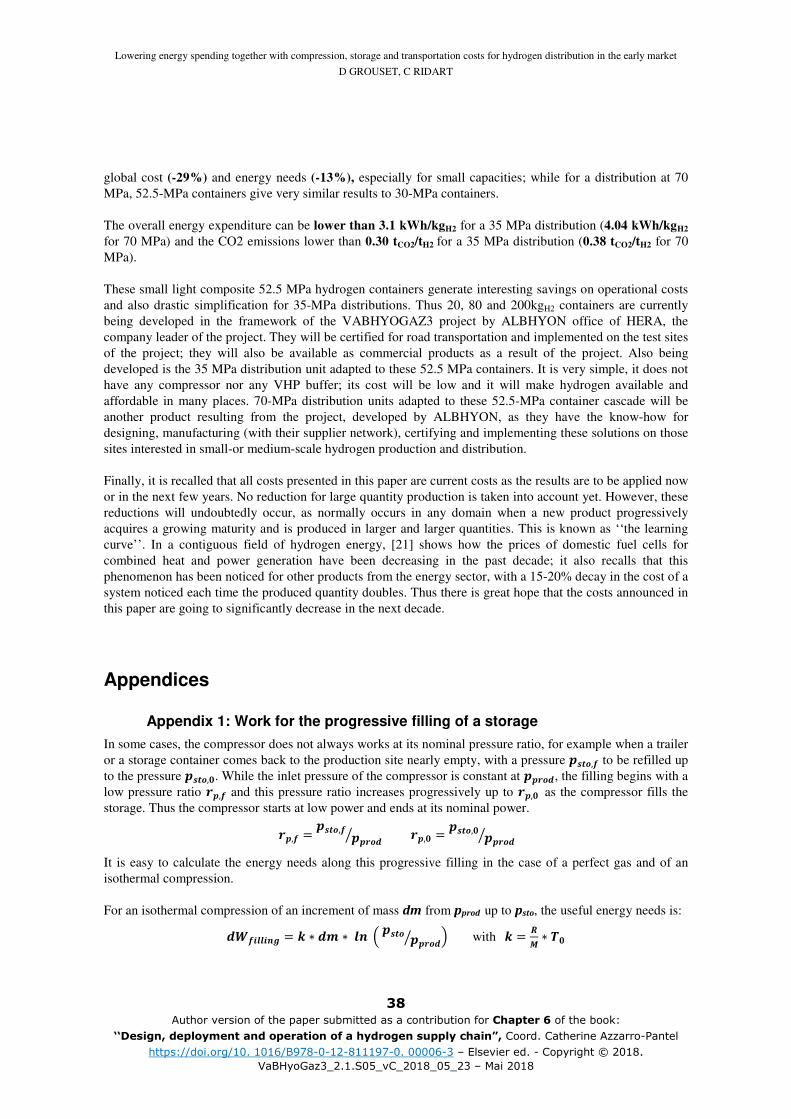
Lowering energy spending together with compression, storage and transportation costs for hydrogen distribution in the early market
D GROUSET, C RIDART
38 Author version of the paper submitted as a contribution for Chapter 6 of the book:
‘‘Design, deployment and operation of a hydrogen supply chain”, Coord. Catherine Azzarro-Pantel https://doi.org/10. 1016/B978-0-12-811197-0. 00006-3 – Elsevier ed. - Copyright © 2018.
VaBHyoGaz3_2.1.S05_vC_2018_05_23 – Mai 2018
global cost (-29%) and energy needs (-13%), especially for small capacities; while for a distribution at 70
MPa, 52.5-MPa containers give very similar results to 30-MPa containers.
The overall energy expenditure can be lower than 3.1 kWh/kgH2 for a 35 MPa distribution (4.04 kWh/kgH2
for 70 MPa) and the CO2 emissions lower than 0.30 tCO2/tH2 for a 35 MPa distribution (0.38 tCO2/tH2 for 70
MPa).
These small light composite 52.5 MPa hydrogen containers generate interesting savings on operational costs
and also drastic simplification for 35-MPa distributions. Thus 20, 80 and 200kgH2 containers are currently
being developed in the framework of the VABHYOGAZ3 project by ALBHYON office of HERA, the
company leader of the project. They will be certified for road transportation and implemented on the test sites
of the project; they will also be available as commercial products as a result of the project. Also being
developed is the 35 MPa distribution unit adapted to these 52.5 MPa containers. It is very simple, it does not
have any compressor nor any VHP buffer; its cost will be low and it will make hydrogen available and
affordable in many places. 70-MPa distribution units adapted to these 52.5-MPa container cascade will be
another product resulting from the project, developed by ALBHYON, as they have the know-how for
designing, manufacturing (with their supplier network), certifying and implementing these solutions on those
sites interested in small-or medium-scale hydrogen production and distribution.
Finally, it is recalled that all costs presented in this paper are current costs as the results are to be applied now
or in the next few years. No reduction for large quantity production is taken into account yet. However, these
reductions will undoubtedly occur, as normally occurs in any domain when a new product progressively
acquires a growing maturity and is produced in larger and larger quantities. This is known as ‘‘the learning
curve’’. In a contiguous field of hydrogen energy, [21] shows how the prices of domestic fuel cells for
combined heat and power generation have been decreasing in the past decade; it also recalls that this
phenomenon has been noticed for other products from the energy sector, with a 15-20% decay in the cost of a
system noticed each time the produced quantity doubles. Thus there is great hope that the costs announced in
this paper are going to significantly decrease in the next decade.
Appendices
Appendix 1: Work for the progressive filling of a storage
In some cases, the compressor does not always works at its nominal pressure ratio, for example when a trailer
or a storage container comes back to the production site nearly empty, with a pressure �-,,� to be refilled up
to the pressure �-,,!. While the inlet pressure of the compressor is constant at ��.,�, the filling begins with a
low pressure ratio .�,� and this pressure ratio increases progressively up to .�,!as the compressor fills the
storage. Thus the compressor starts at low power and ends at its nominal power.
.�,� = �-,,� ��.,�$ .�,! = �-,,! ��.,�$ It is easy to calculate the energy needs along this progressive filling in the case of a perfect gas and of an
isothermal compression.
For an isothermal compression of an increment of mass dm from pprod up to psto, the useful energy needs is:
���+��+�F = E ∗ �� ∗ �� 0�-, ��.,�$ 1 with E = "# ∗ �!

Lowering energy spending together with compression, storage and transportation costs for hydrogen distribution in the early market
D GROUSET, C RIDART
39 Author version of the paper submitted as a contribution for Chapter 6 of the book:
‘‘Design, deployment and operation of a hydrogen supply chain”, Coord. Catherine Azzarro-Pantel https://doi.org/10. 1016/B978-0-12-811197-0. 00006-3 – Elsevier ed. - Copyright © 2018.
VaBHyoGaz3_2.1.S05_vC_2018_05_23 – Mai 2018
The total energy needs to fill the storage from �-,,� to �-,,! from a production unit at ��.,� is equal to the
integral:
��+��+�F = � E ∗ �� ∗ ���-, ��.,�$ ��-,,!
�-, �-,,�
The pressure in the storage in linked to the mass of gas present in the storage: for a perfect gas, an increment
of mass dm induces an isothermal increment of pressure dp linked to the final pressure �-,,! and final
mass �-,,! in the storage: �� �-,,!$ = A�� �-,,!$
��+��+�F = AE ∗ �-,,! �-,,!$ ∗ � �� 0�-, ��.,�$ 1 ∗�-,,!
� �-,,���
Introducing the new variable:
.� = �-, ��.,�$
��+��+�F = AE ∗�-,,! ∗ ��.,� �-,,!$ ∗ � ��4.�5.�! �-,,!��.,�
.� .�,� �-,,���.,�∗ �.�
The primitive function of f(x)=ln(x) is F(x)=x*(ln(x)-1), thus it comes:
��+��+�F = AE ∗ �-,,!/.�,! ∗ `.���.�� − ��a.��.�,! ��+��+�F = E ∗ �-,,!.�,! ∗ b.�,! ∗ 4��4.�,!5 − �5 − .�,� ∗ 4��4.�,�5 − �5c
During this filling, the mass of the storage increases from �-,,! ∗ �-, to �-,,! with:
�-, = �-,,� �-,,!$ = .�,� .�,!$ Thus the transferred mass is �-,,! ∗ � −�-,� and finally the energy needs par unit transferred mass is: ��+��+�F �-./��[ = E ∗ �.�,! ∗ � −�-,� ∗ b.�,! ∗ 4��4.�,!5 − �5 − .�,� ∗ 4��4.�,�5 − �5cOtherwise, this energy for filling a storage with an increasing pressure ratio from .�,� to .�,! can be
compared with the energy for a perfect gas isothermal compression of constant pressure ratio .�,!, which is
eq.3 : �+,-��.�/�,��.���- �$ = E ∗ ��4.�,!5Some numerical values are given in the table A.1, which are used in section D:
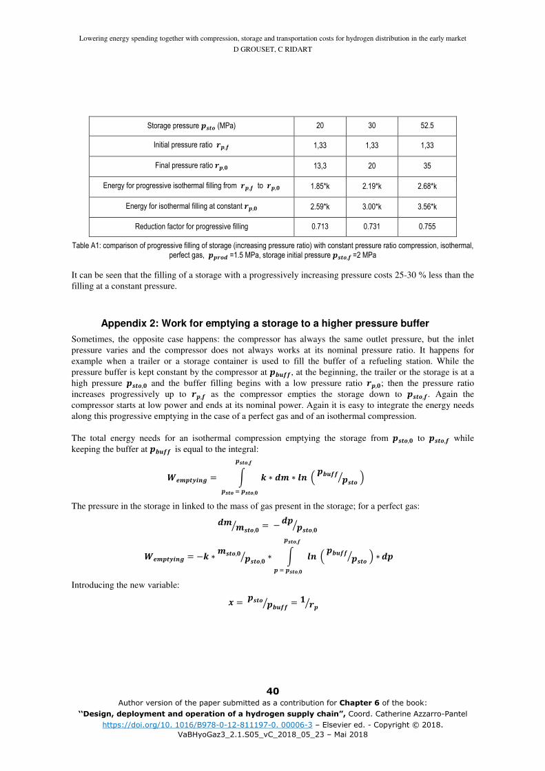
Lowering energy spending together with compression, storage and transportation costs for hydrogen distribution in the early market
D GROUSET, C RIDART
40 Author version of the paper submitted as a contribution for Chapter 6 of the book:
‘‘Design, deployment and operation of a hydrogen supply chain”, Coord. Catherine Azzarro-Pantel https://doi.org/10. 1016/B978-0-12-811197-0. 00006-3 – Elsevier ed. - Copyright © 2018.
VaBHyoGaz3_2.1.S05_vC_2018_05_23 – Mai 2018
Storage pressure �-, (MPa) 20 30 52.5
Initial pressure ratio .�,� 1,33 1,33 1,33
Final pressure ratio.�,! 13,3 20 35
Energy for progressive isothermal filling from .�,� to .�,! 1.85*k 2.19*k 2.68*k
Energy for isothermal filling at constant .�,! 2.59*k 3.00*k 3.56*k
Reduction factor for progressive filling 0.713 0.731 0.755
Table A1: comparison of progressive filling of storage (increasing pressure ratio) with constant pressure ratio compression, isothermal, perfect gas, ��.,� =1.5 MPa, storage initial pressure �-,,�=2 MPa
It can be seen that the filling of a storage with a progressively increasing pressure costs 25-30 % less than the
filling at a constant pressure.
Appendix 2: Work for emptying a storage to a higher pressure buffer
Sometimes, the opposite case happens: the compressor has always the same outlet pressure, but the inlet
pressure varies and the compressor does not always works at its nominal pressure ratio. It happens for
example when a trailer or a storage container is used to fill the buffer of a refueling station. While the
pressure buffer is kept constant by the compressor at �O���, at the beginning, the trailer or the storage is at a
high pressure �-,,! and the buffer filling begins with a low pressure ratio .�,!; then the pressure ratio
increases progressively up to .�,� as the compressor empties the storage down to �-,,�. Again the
compressor starts at low power and ends at its nominal power. Again it is easy to integrate the energy needs
along this progressive emptying in the case of a perfect gas and of an isothermal compression.
The total energy needs for an isothermal compression emptying the storage from �-,,! to �-,,� while
keeping the buffer at �O��� is equal to the integral:
����-G+�F = � E ∗ �� ∗ �� 0�O��� �-,$ 1�-,,�
�-, �-,,!
The pressure in the storage in linked to the mass of gas present in the storage; for a perfect gas: �� �-,,!$ = −�� �-,,!$ ����-G+�F = −E ∗ �-,,! �-,,!$ ∗ � �� 0�O��� �-,$ 1 ∗
�-,,�� �-,,!
��Introducing the new variable:
d = �-, �O���$ = � .�$

Lowering energy spending together with compression, storage and transportation costs for hydrogen distribution in the early market
D GROUSET, C RIDART
41 Author version of the paper submitted as a contribution for Chapter 6 of the book:
‘‘Design, deployment and operation of a hydrogen supply chain”, Coord. Catherine Azzarro-Pantel https://doi.org/10. 1016/B978-0-12-811197-0. 00006-3 – Elsevier ed. - Copyright © 2018.
VaBHyoGaz3_2.1.S05_vC_2018_05_23 – Mai 2018
����-G+�F = AE ∗�-,,! ∗ �O��� �-,,!$ ∗ � ��d�d� �-,,��O���
d d! �-,,!�O���∗ �d
����-G+�F = AE ∗ �-,,! ∗ .�,! ∗ [d��d� − ��]d! � .�,!$d�e� .�,�$
����-G+�F = −E ∗ �-,,!.�,� ∗ b.�,! ∗ 4��4.�,�5 A �5 − .�,� ∗ 4��4.�,!5 A �5cDuring this emptying, the mass of the storage decreases from �-,,! to �-,,! ∗ �-,. Thus the transferred
mass is �-,,! ∗ � −�-,� and finally the energy needs par unit transferred mass is: ����-G+�F �-./��[ = −E ∗ �.�,� ∗ � −�-,� ∗ b.�,! ∗ 4��4.�,�5 A �5 − .�,� ∗ 4��4.�,!5 A �5cOtherwise, this energy for keeping the buffer at its pressure while emptying a storage with an increasing
pressure ratio from .�,f to .�,g can be compared to the energy for a perfect gas isothermal compression in
constant pressure ratio .�,g, which is eq.3.
Some numerical values are given in the table below, which are used in section D:
Buffer pressure �O��� (MPa) 45 90
Nominal storage pressure �-,,! (MPa) 20 30 20 30 52.5
Initial pressure ratio .�,! 2.25 1.5 4.5 3 1.71
Final pressure ratio .�,� 22.5 22.5 45 45 45
Energy for progressive isothermal emptying from .�,! to .�,� 1.56*k 1.21*k 2.25*k 1.90*k 1.41*k
Energy for isothermal emptying at constant .�,!: ��.�,�� 3.11*k 3.11*k 3.81*k 3.81*k 3.81*k
Reduction factor for progressive emptying 0.499 0.389 0.591 0.500 0,370
Table A2: comparison of progressive emptying of storage to fill a buffer (increasing pressure ratio) with constant pressure ratio
compression, isothermal, perfect gas, �O��� =45 or 90MPa, storage final pressure �-,,�=2MPa
It can be seen that emptying a storage with a progressively increasing pressure ratio in order to keep a buffer
at its nominal pressure costs 41-63% less than using the constant high-pressure ratio.
At this stage it is interesting to compare the compression energies in the cases of onsite distribution and of
distant distribution. For the distribution on the production site, only 1 compression is needed, at a constant
high pressure ratio. For a distant distribution, there are 2 compressions, but at increasing pressure ratio, with
lower energy demand, as shown in the table A.3.

Lowering energy spending together with compression, storage and transportation costs for hydrogen distribution in the early market
D GROUSET, C RIDART
42 Author version of the paper submitted as a contribution for Chapter 6 of the book:
‘‘Design, deployment and operation of a hydrogen supply chain”, Coord. Catherine Azzarro-Pantel https://doi.org/10. 1016/B978-0-12-811197-0. 00006-3 – Elsevier ed. - Copyright © 2018.
VaBHyoGaz3_2.1.S05_vC_2018_05_23 – Mai 2018
Onsite dispensing (35 or 70 MPa)
Offsite dispensing (35 or 70 MPa)
Buffer pressure �O��� (MPa) 45 90 45 90
Nominal storage pressure �-,,! (MPa) Without 20 30 20 30 52.5
Compression energy on the production site
3.40*k 4.09*k 1.85*k 2.19*k 1.85*k 2.19*k 2.68*k
Compression energy for dispensing on the distribution site
included included 1.56*k 1.21*k 2.25*k 1.90*k 1.41*k
Total compression energy
3.40*k 4.09*k 3.40*k 3.40*k 4.09*k 4.09*k 4.09*k
Table A3: comparison of the energies for compression: on production site distribution versus off production site distribution; isothermal,
perfect gas, ��.,� =1.5 MPa, storage initial pressure �-,,�=2 MPa
Last line of table A.3 shows that the intermediate step of storage for transportation does not induce any
increase in the compression energy demand, provided the gas is perfect and the compression isothermal.
This result could be intuited, as this calculation is related to the only useful work, with no losses in heating
the gas. It will no longer be the same in the real cases with hydrogen real gas, non-perfectly cooled
compressions and efficiency losses in the compressors…
Appendix 3: Scenario for refueling with several storage units at a higher
initial pressure than the tanks to be filled
In a hydrogen refueling station supplied with transportable containers at a nominal pressure higher than the
nominal pressure of the tanks to be filled (e.g. for example �-,=52.5 MPa for �-/�E=35 MPa), there is no
need for a compressor, nor for high-pressure buffers. But it is necessary to dispose of several storage
containers and these will be returned to the production unit with some residual hydrogen pressure.
This appendix formulates the analytical equations to calculate this residual pressure as a function of the
number of storage containers available at the station. The equations are written for a perfect gas: at any
temperature, pressure and specific mass in the vessel are proportional. This formulation is based on a
scenario in which all vehicles arrive at the station with the same filling state of their tank and are all filled in
the same way from a cascade of storage containers.
Consider the case of 4 storage containers available at the station numbered 1, 2, 3, 4.
Consider a first vehicle with a tank of nominal contained mass �-/�E at nominal pressure �-/�E arriving at
the station with a residual hydrogen pressure and mass �-/�E,!:
�-/�E,! = �-/�E,! ∗ �-/�E �-/�E,! = �-/�E,! ∗ �-/�E Consider this vehicle has been filled to a fraction �-/�E,2 of its nominal mass from storage containers number
4, 3 and 2. It contains a mass �-/�E,2 ∗ �-/�E. Then the storage container 1 complete the filling with a mass 4� − �-/�E,25 ∗ �-/�E up to the pressure �-/�E. The hydrogen mass of storage container 1, which was
initially �-,,!, decreases to �-,,! − 4� − �-/�E,25 ∗ �-/�E while its pressure, initially �-,,! decreases
down to

Lowering energy spending together with compression, storage and transportation costs for hydrogen distribution in the early market
D GROUSET, C RIDART
43 Author version of the paper submitted as a contribution for Chapter 6 of the book:
‘‘Design, deployment and operation of a hydrogen supply chain”, Coord. Catherine Azzarro-Pantel https://doi.org/10. 1016/B978-0-12-811197-0. 00006-3 – Elsevier ed. - Copyright © 2018.
VaBHyoGaz3_2.1.S05_vC_2018_05_23 – Mai 2018
�-,,� = �-,,! ∗ � − 4� − �-/�E,25�-/�E �-,,!$ �=�-,,! ∗ � − 4� − �-/�E,25 ∗ /� with/ = �-/�E �-,,!$
After having filled n such vehicles, the pressure and the mass in the storage container 1 are: �-,,� = �-,,! ∗ � − � ∗ 4� − �-/�E,25 ∗ /��-,,� = �-,,! ∗ � − � ∗ 4� − �-/�E,25 ∗ /�After h vehicles, storage container 1 pressure reaches its minimum value and is connected in the place of
storage container 2: �-,,�,�+� = �-,,%,! = �-,,! ∗ � − h ∗ / ∗ 4� − �-/�E,25��-,,�,�+� = �-,,%,! = �-,,! ∗ � − h ∗ / ∗ 4� − �-/�E,25�Another new storage unit, at full pressure �-,,!, replaces the unit 1; while the unit 2 replaces the unit 3 and
unit 3 replaces the unit 4.
For the first vehicle, within the mass �-/�E,2 ∗ �-/�E the contribution from the storage container 4 and 3
has been �-/�E,% ∗ �-/�E and that of storage container 2 is �-/�E,2 − �-/�E,%� ∗ �-/�E
In the same way, after h other vehicles being filled, pressure and mass in the storage container 2 are: �-,,%,�+� = �-,,2,! = �-,,! ∗ � − h ∗ / ∗ 4� − �-/�E,%5��-,,%,�+� = �-,,2,! = �-,,! ∗ � − h ∗ / ∗ 4� − �-/�E,%5�At that moment a new full storage container at �-,,! is connected at the place of storage container 1 while
storage container 1 is connected at the place of storage container 2; storage container 2 takes the place of
storage container 3 and storage container 3 takes the place of storage container 4.
For these vehicles, within the mass �-/�E,% ∗ �-/�E the contribution from the storage container 4 has been �-/�E,� ∗ �-/�E and that of storage container 3 is �-/�E,% − �-/�E,�� ∗ �-/�E
In the same way, after h other vehicles being filled, pressure and mass in the storage container 3 are: �-,,2,�+� = �-,,),! = �-,,! ∗ � − h ∗ / ∗ 4� − �-/�E,�5��-,,2,�+� = �-,,),! = �-,,! ∗ � − h ∗ / ∗ 4� − �-/�E,�5�At that moment the 3rd permutation takes place, a new full storage container at �-,,! is connected at the place
of storage container 1 while storage container 1 is connected at the place of storage2; storage container 2
takes the place of storage container 3 and storage container 3 the place of storage container 4.
Within the mass �-/�E,� ∗ �-/�E the contribution of the storage container 4 is �-/�E,� − �-/�E,!� ∗ �-/�E
as the vehicle arrived with a residual mass �-/�E,! ∗ �-/�E.
A 4th series of h vehicles is being filled and the residual pressure and mass in storage container 4 are: �-,,),�+� = �-,,.�+�� = �-,,! ∗ � − h ∗ / ∗ 4� − �-/�E,!5��-,,),�+� = �-,,.�+�� = �-,,! ∗ � − h ∗ / ∗ 4� − �-/�E,!5�These are the mass and pressure with which the storage containers are considered empty and returned to the
hydrogen production unit:
�-,,.�+�� = �-,,! ∗ �-, thus � − �-,� = h ∗ / ∗ 4� − �-/�E,!5�

Lowering energy spending together with compression, storage and transportation costs for hydrogen distribution in the early market
D GROUSET, C RIDART
44 Author version of the paper submitted as a contribution for Chapter 6 of the book:
‘‘Design, deployment and operation of a hydrogen supply chain”, Coord. Catherine Azzarro-Pantel https://doi.org/10. 1016/B978-0-12-811197-0. 00006-3 – Elsevier ed. - Copyright © 2018.
VaBHyoGaz3_2.1.S05_vC_2018_05_23 – Mai 2018
� − �-,� is the fraction of hydrogen of the storage container which is effectively used. ) ∗ h is the number
of vehicles which can be served with 4 stages of containers. � is introduced:
� = h ∗ / = � − �-,� � − �-/�E,!�[
At this stage, it can be noticed that it is not necessary all the vehicles have the same tank capacity and the
same filling rate as they arrive to the station. The important is the product h ∗ / or the sum of the /+ from
which their average can be calculated and the average of their filling rate at their arrival to the station:
/i = �hj/+ �-/�E,!333333333 = �hj�-/�E,!,+
Figure A1: schematic diagram for the filling of a tank from a cascade of storage containers � �The values of the coefficients �-/�E,�, �-/�E,%, �-/�E,2 are essential and they cannot be chosen,
they must be calculated considering the constraints on the storage : the storage pressure must be high enough
to ensure the transfer from the storage to the tank, even after the hth vehicle. The overpressure Z��+� is
introduced (fig. A.1). Then the complete set of constraints to consider is: �-,,�,! = �-,,,! �-,,�,�+� = �-,,%,! = �-,,! ∗ � − � ∗ 4� − �-/�E,25�>�-/�E,) ∗ Z��+� = � ∗ �-/�E ∗ Z��+� �-,,%,�+� = �-,,2,! = �-,,! ∗ � − � ∗ 4� − �-/�E,%5�>�-/�E,2 ∗ Z��+� = �-/�E,2 ∗ �-/�E ∗ Z��+��-,,2,�+� = �-,,),! = �-,,! ∗ � − � ∗ 4� − �-/�E,�5�>�-/�E,% ∗ Z��+� = �-/�E,% ∗ �-/�E ∗ Z��+��-,,),�+� = �-,,! ∗ �-, = �-,,! ∗ � − � ∗ 4� − �-/�E,!5�>�-/�E,� ∗ Z��+� = �-/�E,� ∗ �-/�E ∗ Z��+� When replacing the signs > by signs =, 4 equations are obtained, the solution of which allows calculating the
minimum values of the 4 quantities �-/�E,�, �-/�E,%, �-/�E,2 and �-,,!. This means that the residual pressure

Lowering energy spending together with compression, storage and transportation costs for hydrogen distribution in the early market
D GROUSET, C RIDART
45 Author version of the paper submitted as a contribution for Chapter 6 of the book:
‘‘Design, deployment and operation of a hydrogen supply chain”, Coord. Catherine Azzarro-Pantel https://doi.org/10. 1016/B978-0-12-811197-0. 00006-3 – Elsevier ed. - Copyright © 2018.
VaBHyoGaz3_2.1.S05_vC_2018_05_23 – Mai 2018
with which storage containers are returned to the production unit cannot be chosen: it is imposed and highly
sensitive to the quantity �-/�E,!, the average filling rate at which the vehicles arrive at the station.
Another scenario could be considered for refueling. The quantity to transfer to the tank from a given storage
could be not maintained at the same level as the storage pressure decreases. It could be the maximum
possible quantity transferable at any time. Then the first vehicles of the series of the h vehicles would receive
a higher contribution from the storage containers 4 and 3 and a lower contribution from the storage
containers 2 and 1; but the opposite would happen for the last vehicles of the series: the contribution of
storage containers 4 and 3 would be less as their pressure has decreased and storage containers 2 and 1 would
have to complement with a larger contribution. Globally the equation for the definition of � shows that the
same number of vehicles ) ∗ h could be served from the storage containers.
In the case in which only 3 storage containers are available at the station, the same series of equations can be
used. Just do not calculate �-/�E,2 and consider �-/�E,2 = �-/�E,% and �-,,2,�+� = �-,,),�+�
In the case in which only 2 storage containers are available at the station, the same series of equations can be
used. Just do not calculate �-/�E,2 and �-/�E,% and consider: �-/�E,2 = �-/�E,% = �-/�E,�, �-,,%,�+� =�-,,2,�+� = �-,,),�+�
Appendix 4: Scenario for refueling with a compressor, a buffer and several
storage units at a lower initial pressure than the tanks to be filled
In a hydrogen refueling station supplied with transportable containers at a nominal pressure lower than the
nominal pressure of the tanks to be filled, a compressor is mandatory and a very-high-pressure buffers as well
(e.g. �-, =30 MPa and �-/�E =35 MPa with �O��� =45 MPa). This very-high-pressure buffer is filled by the
compressor sucking hydrogen from one of the storage containers and completes the filling of the tanks as the
last stage of the cascade.
The analytical equations have been formulated for the compressor sucking from any storage stage; results
have shown that the contribution of the compressor (the fraction of hydrogen to be compressed) is the lowest
when the compressor sucks from the lowest pressure storage (as in fig. A2). Equations are shown in this case.
The formulation is based on the same scenario as in Appendix 3 and the equations are very similar. The only
differences are:
• The initial pressure of the 2nd storage (for the before last refueling stage) is equal to the nominal
pressure of the full storage �-,,,!,
• � is substituted by �-/�E,2 in the equations: �-,,%,! = �-,,,! �-,,%,�+� = �-,,2,! = �-,,! ∗ � − � ∗ 4�-/�E,2 − �-/�E,%5�>�-/�E,2 ∗ Z��+� = �-/�E,2 ∗ �-/�E ∗ Z��+� �-,,2,�+� = �-,,),! = �-,,! ∗ � − � ∗ 4�-/�E,2 − �-/�E,�5�>�-/�E,% ∗ Z��+� = �-/�E,% ∗ �-/�E ∗ Z��+� �-,,),�+� = �-,,�,! = �-,,! ∗ � − � ∗ 4�-/�E,2 − �-/�E,!5�>�-/�E,� ∗ Z��+� = �-/�E,� ∗ �-/�E ∗ Z��+� �-,,�,�+� = �-,,.�+�� = �-,,! ∗ �-, without any constraint as this storage is feeding the compressor.
When replacing the signs > by signs =, 3 equations are obtained the solution of which allows calculating the
minimum values of the 3 quantities �-/�E,�, �-/�E,%, �-/�E,2. The value of �-,,!, giving the residual pressure
of the storage containers when returned to the production unit, can be chosen. It allows calculating the

Lowering energy spending together with compression, storage and transportation costs for hydrogen distribution in the early market
D GROUSET, C RIDART
46 Author version of the paper submitted as a contribution for Chapter 6 of the book:
‘‘Design, deployment and operation of a hydrogen supply chain”, Coord. Catherine Azzarro-Pantel https://doi.org/10. 1016/B978-0-12-811197-0. 00006-3 – Elsevier ed. - Copyright © 2018.
VaBHyoGaz3_2.1.S05_vC_2018_05_23 – Mai 2018
pressure ratio the compressor must be able to. The value (1-�-/�E,2� is the fraction of the hydrogen to be
compressed (on a total of � − �-/�E,!�).
Figure A2: schematic diagram for the filling of a tank from a cascade of storage containers, a compressor and a very-high-pressure buffer
References
[1] Klell M, Kindermann H, Christian J. Thermodynamics of gaseous and liquid hydrogen storage. In:
Proceedings of IHEC 2007 the International Hydrogen Energy Congress and Exhibition. Istanbul, Turkey 13-
15 July 2007.
http://www.hycenta.tugraz.at/Image/Thermodynamics of gaseous and liquid hydrogen storage.pdf
[2] Schneider J, Suckow T, Lynch F, Ward J, Caldwell M, Tillman J, Mathison S et al. “Optimizing
Hydrogen Vehicle Fueling”. NHA 2005.
http://static1.squarespace.com/static/53ab1feee4b0bef0179a1563/t/543e7eeae4b0983640ec4b93/1413381866
875/NHA+2005+-+Optimizing+Hydrogen+Vehicle+Refueling.pdf
[3] Maus S, Hapke J, Na Ranong C, Wüchner E, Friedlmeier G, Wenger D. Filling procedure for vehicles
with compressed hydrogen tanks. Int J Hydrogen Energy. 2008 Vol.33, No.17, 4612-4621.
[4] SAE International, Surface Vehicle Standard. J2601 Fueling protocols for light duty gaseous hydrogen
surface vehicles. July 2014.
http://www.sae.org/technical/standards/J2601_201407 [5] Mintz M, Elgowainy A, Gardiner M. Rethinking hydrogen fueling: insights from delivery modeling. J. Transp. Res. Board. :2139:46, 2009. [6] Parks G, Boyd R, Cornish J, Remick R. Hydrogen Station Compression, Storage, and Dispensing Technical Status and Costs. NREL Technical Monitor NREL/BK-6A10-58564. May 2014. https://www.nrel.gov/docs/fy14osti/58564.pdf
[7] Rothuizen E, Rokni M. Optimization of the overall energy consumption in cascade fueling stations for
hydrogen vehicles, Int. J. Hydrog. Energy. 39 :582-592, 2014.
https://doi.org/10.1016/j.ijhydene.2013.10.066

Lowering energy spending together with compression, storage and transportation costs for hydrogen distribution in the early market
D GROUSET, C RIDART
47 Author version of the paper submitted as a contribution for Chapter 6 of the book:
‘‘Design, deployment and operation of a hydrogen supply chain”, Coord. Catherine Azzarro-Pantel https://doi.org/10. 1016/B978-0-12-811197-0. 00006-3 – Elsevier ed. - Copyright © 2018.
VaBHyoGaz3_2.1.S05_vC_2018_05_23 – Mai 2018
[8] Reddi K, Elgowainy A, Sutherland E. Hydrogen refueling station compression and storage optimization with tube-trailer deliveries. Int. J. Hydrog. Energy. 39 :19169-19181, 2014,. https://doi.org/10.1016/j.ijhydene.2014.09.099 [9] Wipke K, Sprik S, Kurtz J, Ramsden T, Ainscough C, Saur G. National Fuel Cell Electric Vehicle Learning Demonstration Final Report. National Renewable Energy Laboratory, 2012. http://www.nrel.gov/hydrogen/pdfs/54860.pdf [10] Gardiner M. Energy Requirements for Hydrogen Gas Compression and Liquefaction as Related to Vehicle Storage Needs. U.S. Department of Energy Hydrogen and Fuel Cells Program Record N°9013 July 2009. www.hydrogen.energy.gov/pdfs/9013_energy_requirements_for_hydrogen_gas_compression.pdf
[11] Lemmon E W, Leachman J W. Revised standardized equation for hydrogen densities for fuel
consumption application, J. Res. Natl. Inst. Stand. Technol. 113 :341-350, 2008.
[12] NIST Chemical Webbook, n.d.
http://webbook.nist.gov/chemistry/fluid, last consulted dec 2017 [13] Nexant Inc., Air Liquide, Argonne National Laboratory, Chevron Technology Venture, Gas Technology Institute, National Renewable Energy Laboratory, Pacific Northwest National Laboratory, TIAX LLC. H2A: Hydrogen delivery infrastructure analysis models and conventional pathway options analysis results. Report DE-FG36-05GO15032. DOE. May 2008. www1.eere.energy.gov/hydrogenandfuelcells/pdfs/nexant_h2a.pdf
[14] Smith R. Chemical process. :273, ed. John Wiley & Sons New York, 2005 [15] Bourgeois T, Brachmann T, Barth F, Ammouri F, Baraldi D, Melideo D, Acosta-Iborra B, Zaepffel D, Saury D, Lemonnier D. Optimization of hydrogen vehicle refuelling requirements. Int. J. Hydrog. Energy 1-21, 2017 http://dx.doi.org/10.1016/j.ijhydene.2017.01.165 [16] Bourgeois T, Ammouri F, Weber M, Knapik C. Evaluating the temperature inside a tank during a filling with highly pressurized gas. Int. J. Hydrog. Energy 40 :11748-55, 2015. [17] L Zhao, Y Liu, J Yang, Y Zhao, J Zheng, H Bie, X Liu. Numerical simulation of temperature rise within hydrogen vehicle cylinder during refueling. Int. J. Hydrog. Energy 35 :8092-8100, 2010. https://doi.org/10.1016/j.ijhydene.2010.01.027 [18] Woodfield PL, Monde M, Mitsutake Y. Measurement of averaged heat transfer coefficients in high-pressure vessel during charging with hydrogen, nitrogen or argon gas. J. Therm. Sci. Technol. 2(2): 180-91, 2007. [19] Monde M, Mitsutake Y, Woodfield P, Maruyama. Characteristics of heat transfer and temperature rise of hydrogen during rapid hydrogen filling at high pressure. Heat Transfer Asian Research 36(1) :13-27, 2007 [20] Lee S, Kim Y, Kim S, Yoon K. Temperature change of a type IV cylinder during hydrogen fueling process. In: Proceedings of the International conference on hydrogen safety, Ajaccio; 2009. [21] Staffell I, Green R. The cost of domestic fuel cell micro-CHP systems. Imperial College Business Scholl of London, UK. Int. J. Hydrog. Energy. 38-2 :1088-1102, 2013. https://doi.org/10.1016/j.ijhydene.2012.10.090 Total : 19451 mots et 47 pages WORD ;19050 mots et 46 pages hors ABSTRACT