Intrathecal Drug Targeting: Distribution of Opioids in the Spinal CanalNirav Soni

nsoni6@uic.eduThis report is produced under the supervision of BIOE 310 instructor Professor Linninger

Abstract

Intrathecal opioid application is a method used to treat many diseases, such as chronic pain and spinal cancer 1,2,3. However, the mechanisms of biodistribution for drugs administered in the cerebrospinal fluid (CSF) are not well understood in academia. This project aims at creating a mechanistic model through three different models of flow to prove the spread of the drugs in the subarachnoid space is patient specific and depends on the pharmacokinetic parameters of each opioid4,5. A variety of conservation balance equations will be used in order to describe the direction of incoming and outgoing flow throughout this network, the pressure drop throughout different spinal compartments, the change in volume throughout the network, and the concentration of four different opioids at different positions throughout the intrathecal space. The mechanistic model of the spinal canal will be imaged in order to guide the mathematical studies of the effects of pulsatile CSF flow on each opioid. The models formed through MATLAB compute spinal distribution of the opioids, absorption of the drugs into the spinal cord, epidural tissue, and vasculature, blood clearance for different injection locations, and number and duration of the injections. In order to illustrate intrathecal drug targeting, plots of flow, volume, pressure, and concentration were created with respect to a bolus injection for each opioid. When studying the figures produced through each of the three flow models, the results support the hypothesis by showing the differences in pressure, volume, flow, and concentration by bolus injections for the different opioids selected.

1. Introduction

Intrathecal drug delivery is a clinical treatment option for many diseases, including spinal cancer and chronic pain1,2,3. This process consists of direct drug injection into the spinal canal where the flow of CSF allows for a natural drug transport2,3. Because the medication is delivered directly to the spinal cord, it can be more effective than taking oral medications, which must travel through other systems before reaching the spine. 

Recently, researchers at the University of Illinois at Chicago have discovered the important role of CSF amplitude and frequency for the rapid dispersion after intrathecal administration6. The extent of drug distribution in vivo is highly variable and difficult to control. Varying CSF pulsatility and heart rate from patient to patient may lead to different drug distribution6. Computations in contemporary experiments demonstrate that the speed of drug transport is strongly affected by the frequency and magnitude of CSF pulsations.

Some opioids used in intrathecal delivery include morphine, fentanyl, alfentanil, and sufentanil4. Current studies have sampled the spinal cord, CSF and epidural space after intrathecal injections of these drugs in order to characterize the rate and extent of opioid distribution4. This information can be used to demonstrate different pharmacokinetic behavior,

which correlates well with their pharmacodynamic behavior4,5.

When rationalizing choice of drug, computer simulations in recent studies provide insight into the comparative pharmacokinetics that can be used to select the appropriate opioid based on the length of the procedure, the desired intraoperative opioid concentration, and the desired time course of recovery5. Opioid selection requires acknowledgement of the relationship between the pharmacokinetic and pharmacodynamics characteristics of these drugs and the onset of and recovery from drug effect5.

In order to create a mathematical model, which represents the illustration below (Figure 1), to predict the natural intrathecal transport of the opioids, multiple variables must be accounted for. When considering spinal distribution of the drug, absorption rate of the drug into the tissue, blood clearance for different injection locations, number and duration of the injections, and choice of drug must be studied.

Figure 1:Intrathecal Injection Illustration. Opioid injection made in the lumbar region, L2, of the spinal cord 6.

2. Methods

Conservation balance equations are essential when describing the physical world. In order to numerically illustrate the flow network shown in Figure 2, algebraic and differential systems of equations were formulated using the following mathematical equations:

Three different models of flow were used to solve the small flow network. The flow network follows the relationship given by Equations 1, 2, and 3. In order to establish a standard, the arrival of flow into a node was noted with positive pressures, whereas the departure of flow was denoted with negative pressures.

d U i

dt=Pi−Pi+1+α iU i (1)

d U i

dt=[U i−1

2

2+

Pi

ρ ]−[U i+12

2+

Pi+1

ρ ]+α iU i (2)

d U i

dt=[U i−1

2

2+

Pi

ρ ]−[ U i2

2+

Pi +1

ρ ]+αi U i (3)

Flow conservation equations, given by Equation 4, were used in order to describe the direction of incoming and outgoing flow throughout the intrathecal space. The incoming flow was denoted with a positive value whereas the outgoing flow was given a negative value.

dV i

dt=F

i−F i+1 (4)

Compressibility equations, given by Equation 5, were formulated in order to relate relative change in volume of the CSF as a response to the change in

pressure. This will help describe the deformation in the flow network.

dV i

dt=K

d Pi

dt (5)

Species balance equations, given by Equation 6, were used in order to map the concentration of each opioid with respect to time at the brain, cervical, thoracic, lumbar, and sacral regions.

Vd C i

dt=F iC i−F i+1 Ci+1−k C i (6)

In order to simplify computations within Matlab Code 2 for the purpose of creating a mechanistic model of the flow network, Equation 7 was derived using a combination of the previous equations.

Kd Pi

dt= 1

αi−1(Pi−1−Pi)− 1

αi(Pi−Pi+1)

(7)

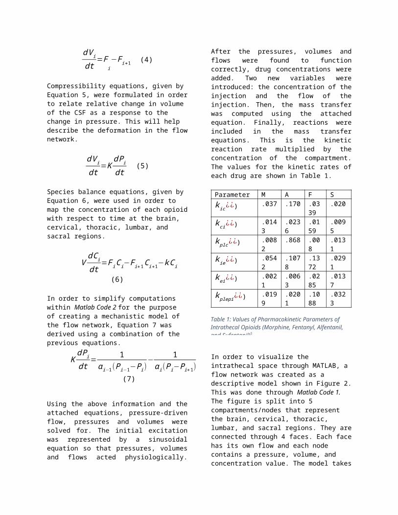
Using the above information and the attached equations, pressure-driven flow, pressures and volumes were solved for. The initial excitation was represented by a sinusoidal equation so that pressures, volumes and flows acted physiologically. After the pressures, volumes and flows were found to function correctly, drug concentrations were added. Two new variables were introduced: the concentration of the injection and the flow of the injection. Then, the mass transfer was computed using the attached equation. Finally, reactions were included in the mass transfer equations. This is the kinetic reaction rate multiplied by the concentration of the compartment. The values for the kinetic rates of each drug are shown in Table 1.

Parameter M A F Sk ic¿¿) .037 .170 .0339 .020

k ci¿¿) .0143 .0236 .0159 .0095

k plc ¿¿) .0082 .868 .008 .0131

k ie ¿¿) .0542 .1078 .1372 .0291

k ei¿¿) .0021 .0063 .0285 .0137

k plepi ¿¿) .0199 .0201 .1088 .0323

Table 1: Values of Pharmacokinetic Parameters of Intrathecal Opioids (Morphine, Fentanyl, Alfentanil, and Sufentanil)5.

In order to visualize the intrathecal space through MATLAB, a flow network was created as a descriptive model shown in Figure 2. This was done through Matlab Code 1. The figure is split into 5 compartments/nodes that represent the brain, cervical, thoracic, lumbar, and sacral regions. They are connected through 4 faces. Each face has its own flow and each node contains a pressure, volume, and concentration value. The model takes into account the spread of opioids into the CSF, spinal cord, epidural tissue, and vasculature. Figure 2 was created through labeling and drawing shapes though built in MATLAB commands: viscircles, line, and text.

-5 0 5 10 15 20 25 30 35 400

5

10

15

20

25

30

35

V2

P1

F1

V3

P2

F2

V4

P3

F3

V5

P4

F4

P5

Brain

Cervical

Thoracic

Lumbar

Sacral

V1

Spinal Cord Model

Epi

dura

l Spa

ce

Vas

cula

ture

This figure was essential when determining the equations for the different models of flow, volume, pressure, and concentration.

In order to solve for pressure-driven flow, volume, pressure, and concentration, Matlab Code 2 was created. This was done through the creation of functions. First off, a matrix y0 was created containing the initial values for: volume, pressure, morphine concentration, fentanyl concentration, afentanil concentration, and sufentanil concentration. Compression constant and resistance and kinetic values for were determined through literature5. Initial pressure was realized to be a sinusoidal function due to its relationship to the pulsatile flow of CSF in the spinal canal. A sinusoidal function was used in order to create a physiologically accurate model. Pressure-driven flows were solved for by the use of three

different flow models represented in Equation 1, Equation 2, and Equation 3 at each face for its corresponding flow. Flows were plotted in a bolus injection. Volume was solved for using Equation 4 for each corresponding node. Volume was plotted in a bolus injection. Pressure was solved for through the use of Equation 5 and the realization that pressure is the derivative of volume. Pressure was plotted in a bolus injection. After flow, volume, and pressure was found, the next step was to solve for drug concentration. Two new variables were introduced: the concentration of the injection and the flow of the injection. The flow of the injection was inserted into the volume equations. Concentrations were solved for using the built-in MATLAB function max. Max was used in order to determine which way flow was going at a given point. Reactions were then included in the mass transfer equations through the use of kinetic rates, k, of each drug. In order to compute the results for both a bolus injection, an if-else loops was utilized in order to determine a value for injection flow and injection concentration in the lumbar region based on the time of injection.

3. Results

Plots of flows, volumes, pressures, and concentrations were produced through the use of Matlab Code 2. The graphs produced take into account all four opioids (Morphine, Fentanyl, Afentanil, and Sufentanil) introduced through a bolus injection.

3.1 Model 1

Figure 3 illustrates Model 1 flows through each phase of the flow network for a 50 mL bolus injection of opioid occurring at 5 seconds. The highest amplitude of pulsatile motion is seen to occur at the injection site between the Lumbar and Sacral region (L2).

Figure 2: Intrathecal Flow Network: Flows (F) 1-4 represented at the faces of the flow network. Pressures (P) and Volumes (V) 1-5 represented at each node of the network. The concentration of the opioid spreads to the epidural tissue and to vasculature

Figure 3: Flows 1-4 through each face of the flow network after a bolus injection with respect to time.

Figure 4 shows the volume at each compartment of the flow network throughout a range of time for a bolus injection. The volume at the brain (55 mL) is much larger than any other region. It can be observed that the volume with respect to time is oscillatory due to the biological properties of the flow of CSF in the intrathecal space.

Figure 4: Volume levels in the brain (55 mL) and spinal compartments (23 mL, 33 mL, 25 mL, 19 mL) in order of Cervical, Thoracic, Lumbar, and Sacral.

Figure 5 illustrates the pressures at each compartment of the intrathecal flow model throughout a range of time for a bolus injection. It can be seen that the pressure increases due to the injection at the Lumbar region (L2).

Figure 5: Pressure in the brain and each spinal compartment after a bolus injection with respect to time.

Figure 6 represents the concentration of Morphine (top left), Alfentanil (top right), Fentanyl (bottom left), and Sufentanil (bottom right) in the CSF space at each compartment throughout a range of time after a bolus injection. The injection starts at 5 seconds. It is seen that at the injection time all of the opioid drug concentrations are highest in the Lumbar region (L2) and that they are distributed throughout the intrathecal space.

Figure 6: Concentration of each opioid at each spinal compartment in the CSF space with respect to time.

Figure 7 represents the concentration of Morphine (top left), Alfentanil (top right), Fentanyl (bottom left), and Sufentanil (bottom right) in the spinal cord throughout a range of time after a bolus injection. The injection starts at 5 seconds. It is seen that each drug throughout time is approaching an equilibrium concentration.

Figure 7: Concentration of each opioid in different regions of the spinal cord with respect to time.

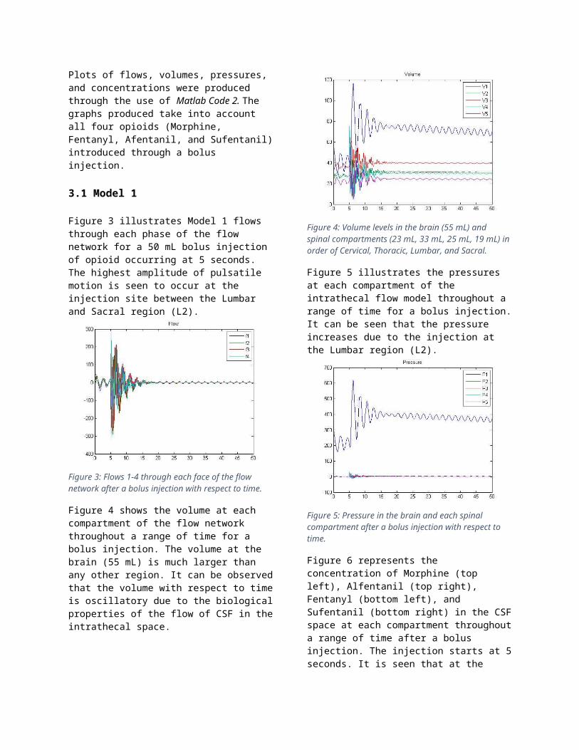
Figure 8 represents the concentration of Morphine (top left), Alfentanil (top right), Fentanyl (bottom left), and Sufentanil (bottom right) in the epidural tissue throughout a range of time after a bolus injection. The injection starts at 5 seconds. It is seen that each drug throughout time is approaching an equilibrium concentration.

Figure 8: Concentration of each opioid in different regions of the epidural tissue with respect to time.

Figure 9 represents the concentration of Morphine (top left), Alfentanil (top right), Fentanyl (bottom left), and Sufentanil (bottom right) in vasculature throughout a range of time after a bolus injection. The injection starts at 5 seconds. It is seen that each drug within the range of time is increasing and will approach an equilibrium concentration.

Figure 9: Concentration of each opioid in different regions of vasculature with respect to time.

3.2 Model 2

Figure 10 illustrates Model 2 flows through each phase of the flow network for a 50 mL bolus injection of opioid occurring at 5 seconds. The highest amplitude of pulsatile motion is seen to occur at the injection site between the Lumbar and Sacral region (L2).

Figure 10: Flows 1-4 through each face of the flow network after a bolus injection with respect to time.

Figure 11 shows the volume at each compartment of the flow network throughout a range of time for a bolus injection. The volume at the brain (55 mL) is much larger than any other region. It can be observed that the volume with respect to time is oscillatory due to the biological properties of the flow of CSF in the intrathecal space.

Figure 11: Volume levels in the brain (55 mL) and spinal compartments (23 mL, 33 mL, 25 mL, 19 mL) in order of Cervical, Thoracic, Lumbar, and Sacral.

Figure 12 illustrates the pressures at each compartment of the intrathecal flow model throughout a range of time for a bolus injection. It can be seen that the pressure increases due to the injection at the Lumbar region (L2).

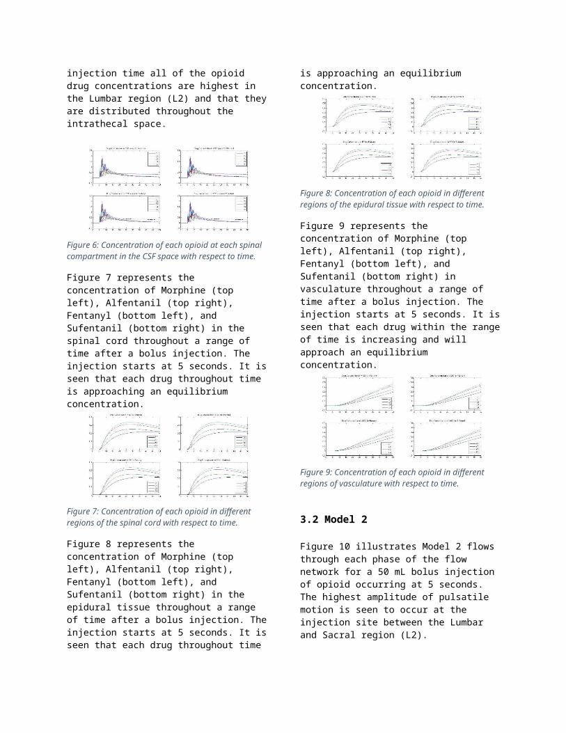
Figure 12: Pressure in the brain and each spinal compartment after a bolus injection with respect to time.

Figure 13 represents the concentration of Morphine (top left), Alfentanil (top right), Fentanyl (bottom left), and Sufentanil (bottom right) in the CSF space at each compartment throughout a range of time after a bolus injection. The injection starts at 5 seconds. It is seen that at the injection time all of the opioid drug concentrations are highest in the Lumbar region (L2) and that they are distributed throughout the intrathecal space.

Figure 13: Concentration of each opioid at each spinal compartment in the CSF space with respect to time.

Figure 14 represents the concentration of Morphine (top left), Alfentanil (top right), Fentanyl (bottom left), and Sufentanil (bottom right) in the spinal cord throughout a range of time after a bolus injection. The injection starts at 5 seconds. It is seen that each drug throughout time is approaching an equilibrium concentration.

Figure 14: Concentration of each opioid in different regions of the spinal cord with respect to time.

Figure 15 represents the concentration of Morphine (top left), Alfentanil (top right), Fentanyl (bottom left), and Sufentanil (bottom right) in the epidural tissue throughout a range of time after a bolus injection. The injection starts at 5 seconds. It is seen that each drug throughout time is approaching an equilibrium concentration.

Figure 15: Concentration of each opioid in different regions of the epidural tissue with respect to time.

Figure 16 represents the concentration of Morphine (top left), Alfentanil (top right), Fentanyl (bottom left), and Sufentanil (bottom right) in vasculature throughout a range of time after a bolus injection. The injection starts at 5 seconds. It is seen that each drug within the range of time is increasing and will approach an equilibrium concentration.

Figure 16: Concentration of each opioid in different regions of vasculature with respect to time.

3.3 Model 3

Figure 17 illustrates Model 3 flows through each phase of the flow network for a 50 mL bolus injection of opioid occurring at 5 seconds. The highest amplitude of pulsatile motion is seen to occur at the injection site between the Lumbar and Sacral region (L2).

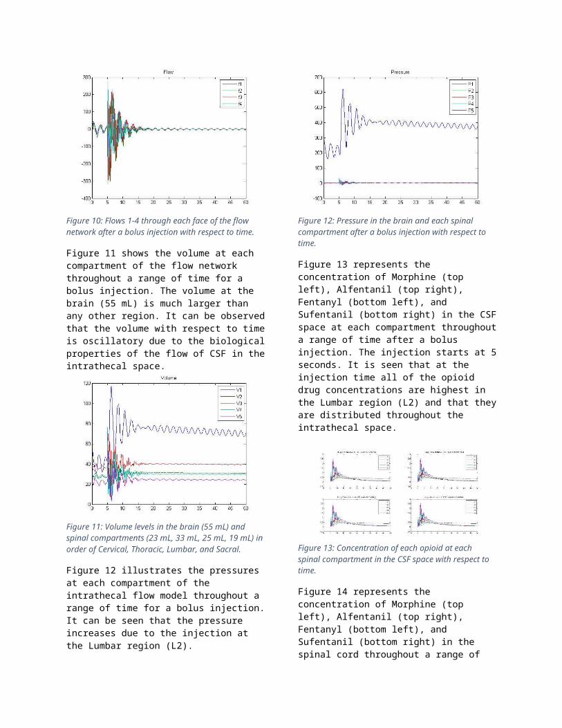
Figure 17: Flows 1-4 through each face of the flow network after a bolus injection with respect to time.

Figure 18 shows the volume at each compartment of the flow network throughout a range of time for a bolus injection. The volume at the brain (55 mL) is much larger than any other region. It can be observed that the volume with respect to time is oscillatory due to the biological properties of the flow of CSF in the intrathecal space.

Figure 18: Volume levels in the brain (55 mL) and spinal compartments (23 mL, 33 mL, 25 mL, 19 mL) in order of Cervical, Thoracic, Lumbar, and Sacral.

Figure 19 illustrates the pressures at each compartment of the intrathecal flow model throughout a range of time for a bolus injection. It can be seen that the pressure increases due to the injection at the Lumbar region (L2).

Figure 19: Pressure in the brain and each spinal compartment after a bolus injection with respect to time.

Figure 20 represents the concentration of Morphine (top left), Alfentanil (top right), Fentanyl (bottom left), and Sufentanil (bottom right) in the CSF space at each compartment throughout a range of time after a bolus injection. The injection starts at 5 seconds. It is seen that at the injection time all of the opioid drug concentrations are highest in the Lumbar region (L2) and that they are distributed throughout the intrathecal space.

Figure 20: Concentration of each opioid at each spinal compartment in the CSF space with respect to time.

Figure 21 represents the concentration of Morphine (top left), Alfentanil (top right), Fentanyl (bottom left), and Sufentanil (bottom right) in the spinal cord throughout a range of time after a bolus injection. The injection starts at 5 seconds. It is seen that each drug throughout time is approaching an equilibrium concentration.

Figure 21: Concentration of each opioid in different regions of the spinal cord with respect to time.

Figure 22 represents the concentration of Morphine (top left), Alfentanil (top right), Fentanyl (bottom left), and Sufentanil (bottom right) in the epidural tissue throughout a range of time after a bolus injection. The injection starts at 5 seconds. It is seen that each drug throughout time is approaching an equilibrium concentration.

Figure 22: Concentration of each opioid in different regions of the epidural tissue with respect to time.

Figure 23 represents the concentration of Morphine (top left), Alfentanil (top right), Fentanyl (bottom left), and Sufentanil (bottom right) in vasculature throughout a range of time after a bolus injection. The injection starts at 5 seconds. It is seen that each drug within the range of time is increasing and will approach an equilibrium concentration.

Figure 23: Concentration of each opioid in different regions of vasculature with respect to time.

3.4 Model Comparison

As shown in the Figure 24, the three different models of flow are plotted on top of one another in different colors. Model 1 is blue, Model 2 is red, and Model 3 is black. This is to demonstrate the similarities and differences between the models. It is seen that

although they follow a similar trend, there are noticeable differences between each model.

Figure 10: Comparison between the three models of flow (Model 1= blue, Model 2=red, Model 3= black) for a bolus injection of Morphine with respect to time.

4. Discussion

In the mechanistic models of the intrathecal flow network, the effects of each opioid injection within the system were projected with respect to concentration with reactions and mass transfer. Initially at the injection time, the highest concentration occurred in the in the lumbar vertebrae, due to the injection site being located at L2. A phase lag was witnessed between the flows at each phase and the volume, pressure, and concentration at each compartment. The compartments with a significantly smaller flow experienced a slower distribution of CSF volume which resulted in a lower opioid concentration throughout a range of time. The compartments with a significantly higher flow experienced a faster distribution of CSF volume which resulted in a higher opioid concentration throughout a range of time. The brain received a fair amount of the selected opioid due to the higher level of pulsatile flow in that regions when compared to the vertebrate.

It is seen that the flow at each face from the brain to the sacral vertebrate decreases significantly throughout. This information is essential when solving for pressure and volume within each region of the intrathecal flow network.

As the model shows, the pressure occurred to be highest in the brain and lowest in the sacral region for a bolus injection. This can be confirmed mathematically through the use of the three flow models (Equation 1, 2, and 3). Due to the flow being highest near the brain, the pressure will be the highest in the brain. The pressure will be the lowest at the sacral vertebrate due to the flow being lowest in the sacral region.

Understandably, the volume of CSF in the brain is the highest in order for the drug to disperse

adequately. It is given in literature that the initial volume of CSF in the brain is measured to be about 55 mL while the individual vertebra of the human spinal cord ranged from 19 mL to 33 mL7. The figures also show that both volume and pressure at each compartment in the flow network have an oscillatory behavior due to the pulsatile flow of CSF.

For each graph of flow, volume and pressure within each of the three different flow models, it is evident that the initial sinusoidal pressure affects each flow, volume and pressure in every compartment due to their corresponding sinusoidal qualities. This is clearly illustrated through the different degree of oscillations at each node. It is also seen that the concentrations of the drugs oscillate throughout the network due to them being affected by the initial sinusoidal pressure caused by the pulsatile flow of CSF.

It is shown in Figure 24 that although each of the three flow models are noticeably different, they follow the same trend and any one of them can be used when modeling intrathecal drug distribution.

The dispersion of the concentration of the drug increased with respect to time. This mechanistic models demonstrate how the opioids will behave throughout the intrathecal flow network. Variables can be changed by researchers to provide a more applicable model.

5. Conclusion

The computations performed and the mechanistic models created have demonstrated that there are a variety of factors that need to be accounted for in intrathecal drug delivery. It has been determined that drug distribution is patient specific due to the resistance being affected by the length and diameter of the spinal cord along with the viscosity of CSF. Also, it has been established that drug distribution depends on the choice of the opioid as a result of the varying kinetic values of pharmacokinetic parameters. With the creation of these mechanistic models, engineers and researchers can now further study the mechanisms of biodistribution for drugs administered in the CSF

Acknowledgement

This project was assigned in the Biological Systems Analysis course at the University of Illinois at Chicago in the Fall semester of 2014 under the instruction of Professor Andreas Linninger. It was completed with the help of Chih-Yang Hsu and Sebastian Pernal.

Intellectual Property

Biological and physiological data and some modeling procedures provided to you from Dr. Linninger’s lab are subject to IRB review procedures and Intellectual property procedures. Therefore, the use of these data and procedures are limited to the coursework only. Publications need to be approved and require joint authorship with staff of Dr. Linninger’s lab.

References

1. Smith, Thomas J., et al. "Randomized clinical trial of an implantable drug delivery system compared with comprehensive medical management for refractory cancer pain: impact on pain, drug-related toxicity, and survival."Journal of Clinical Oncology 20.19 (2002): 4040-4049.

2. Stearns, Lisa, et al. "Intrathecal drug delivery for the management of cancer pain." J Support Oncol 3 (2005): 399-408.

3. Smith, Howard S., et al. "Intrathecal drug delivery." Pain Physician 11.2 Suppl (2008): S89-S104.4. Ummenhofer, Wolfgang C., et al. "Comparative spinal distribution and clearance kinetics of intrathecally

administered morphine, fentanyl, alfentanil, and sufentanil." Anesthesiology 92.3 (2000): 739-753.5. Shafer, Steven L., and John R. Varvel. "Pharmacokinetics, pharmacodynamics, and rational opioid

selection." Anesthesiology 74.1 (1991): 53-63.6. Hsu, Ying, et al. "The frequency and magnitude of cerebrospinal fluid pulsations influence intrathecal drug

distribution: key factors for interpatient variability." Anesthesia & Analgesia 115.2 (2012): 386-3947. Agamanolis, Dimitri P., M.D. “Chapter 14.” Cerebrospinal Fluid. Neuropathology, Jan.-Feb. 2013. Web.

04 Dec. 2014.

Appendix

Matlab Code 1: Brain Model

clear all, close all, clc %% normal/ idealfor i = 1:2:3 subplot(1,3,i) C = [7.5, 26; 7.5, 18; 7.5, 10; 7.5, 2 7.5, -6]; Lx = [7.5, 7.5; 7.5, 7.5; 7.5, 7.5; 7.5, 7.5 7.5, 7.5]; Ly = [32, 28; 24, 20; 16, 12; 8, 4 0, -4]; %labelingfor i = 1:4 c = C(i,1)-1; cP = C(i,1)-5; text(c, C(i,2), ['V', num2str(i+1)]) cLx = C(i,1)+3; cLy = C(i,2)+4;

text(cLx, C(i,2)+8, ['P', num2str(i)]) text(cLx, cLy, ['F', num2str(i)]) if i == 4 cLx = C(i+1,1)+3; cLy = C(i+1,2)+8; text(cLx, cLy, ['P', num2str(i+1)]) endend %flow lines for i = 1:4 line(Lx(i,:), Ly(i,:), 'Color', 'k') end %labelingtext(6, 35, 'Brain')text(0, C(1,2), 'Cervical')text(0, C(2,2), 'Thoracic')text(0, C(3,2), 'Lumbar')text(0, C(4,2), 'Sacral')text(6, 33, 'V1')axis([0 15 0 37])title('Spinal Cord Model') %brain rectangleRx = [5; 10; 10; 5; 5];Ry = [32; 32; 37; 37; 32];line(Rx, Ry, 'Color', 'k') C = [7.5, 26; 7.5, 18; 7.5, 10; 7.5, 2 7.5, -6];r = [2; 2; 2; 2]; %compartments viscircles(C(1:4, :), r, 'Edgecolor', 'k', 'LineWidth', 1)axis equalend %% deformationsubplot(1,3,2) C = [7.5, 26; 7.5, 18; 7.5, 10; 7.5, 2 7.5, -6]; Lx = [7.5, 7.5; 7.5, 7.5; 7.5, 7.5; 7.5, 7.5

7.5, 7.5]; Ly = [32, 29.5; 22.5, 21; 15, 12.5; 7.5, 4 0, -4]; %labelingfor i = 1:4 c = C(i,1)-1; cP = C(i,1)-5; text(c+0.5, C(i,2), ['V', num2str(i+1)]) cLx = C(i,1)+3; cLy = C(i,2)+4; text(cLx+1, C(i,2)+8, ['P', num2str(i)]) text(cLx+1, cLy, ['F', num2str(i)]) if i == 4 cLx = C(i+1,1)+4; cLy = C(i+1,2)+8; text(cLx, cLy, ['P', num2str(i+1)]) endend for i = 1:4 line(Lx(i,:), Ly(i,:), 'Color', 'k') %flow lines end %labelingtext(6.5, 35, 'Brain')text(0, C(1,2), 'Cervical')text(0, C(2,2), 'Thoracic')text(0, C(3,2), 'Lumbar')text(0, C(4,2), 'Sacral')text(7, 33, 'V1')axis([0 15 0 37])title('Spinal Cord Model with Deformation') Rx = [5; 10; 10; 5; 5];Ry = [32; 32; 37; 37; 32]; line(Rx, Ry, 'Color', 'k') %brain rectangle C = [7.5, 26; 7.5, 18; 7.5, 10; 7.5, 2 7.5, -6];r = [3.5; 3; 2.5; 2]; %compartmentsviscircles(C(1:4, :), r, 'Edgecolor', 'k', 'LineWidth', 1)

%% Full modelfigure C = [7.5, 26; 7.5, 18; 7.5, 10; 7.5, 2 7.5, -6]; Lx = [7.5, 7.5; 7.5, 7.5; 7.5, 7.5; 7.5, 7.5 7.5, 7.5]; Ly = [32, 28; 24, 20; 16, 12; 8, 4 0, -4]; %labeling for i = 1:4 c = C(i,1)-1; cP = C(i,1)-5; text(c, C(i,2), ['V', num2str(i+1)]) cLx = C(i,1)+3; cLy = C(i,2)+4; text(cLx, C(i,2)+9, ['P', num2str(i)]) text(cLx, cLy, ['F', num2str(i)]) if i == 4 cLx = C(i+1,1)+3; cLy = C(i+1,2)+8; text(cLx, cLy+1, ['P', num2str(i+1)]) endend for i = 1:4 line(Lx(i,:), Ly(i,:), 'Color', 'k') %flow line downward end %labelingtext(6, 35, 'Brain')text(0, C(1,2), 'Cervical')text(0, C(2,2), 'Thoracic')text(0, C(3,2), 'Lumbar')text(0, C(4,2), 'Sacral')text(6, 33, 'V1')axis([0 15 0 37])title('Spinal Cord Model') Rx = [5; 10; 10; 5; 5];Ry = [32; 32; 37; 37; 32];line(Rx, Ry, 'Color', 'k') %brain rectangle

RLx = [9.5; 15];RLy = [26; 26; 18; 18; 10; 10; 2; 2];for i = 2:2:8line(RLx, RLy(i-1:i), 'Color', 'k') %line to epidural spaceend Bx = [15; 20; 20; 15; 15];By = [0; 0; 28; 28; 0];line(Bx, By, 'Color', 'k') %epidural space boxh = text(17.5,12, 'Epidural Space');set(h, 'rotation', 90) line([20; 25], [18; 18], 'Color', 'k') %line to vasculature Bx = [25; 30; 30; 25; 25];By = [0; 0; 28; 28; 0];line(Bx, By, 'Color', 'k') %vasculature boxh = text(27.5,12,'Vasculature');set(h, 'rotation', 90) C = [7.5, 26; 7.5, 18; 7.5, 10; 7.5, 2 7.5, -6];r = [2; 2; 2; 2]; viscircles(C(1:4, :), r, 'Edgecolor', 'k', 'LineWidth', 1) %compartmentsaxis equal

Matlab Code 2: Brain ODE

function nsonip()clear all; close all; clc;y0 = zeros(30,1);y0(1:5)=[55;23;33;25;19]; global jfor j = 1:4 [T,Y] = ode45(@brainwaiver ,[0 50],y0); V = Y(:,1:5);P = .0075*Y(:,6:9);P0 =V(:,1)/.188;F = Y(:,10:13); c = ['b';'k';'r'];plot(T,F)%,c(i))hold on if j ==1

TM=T; CM = Y(:,14:18);CMsc = Y(:,19:22); CMepi = Y(:,23:26);CMvas = Y(:,27:30);end if j ==2TA=T; CA = Y(:,14:18);CAsc = Y(:,19:22); CAepi = Y(:,23:26);CAvas = Y(:,27:30);end if j ==3TF=T; CF = Y(:,14:18);CFsc = Y(:,19:22); CFepi = Y(:,23:26);CFvas = Y(:,27:30);end if j ==4TS=T; CS = Y(:,14:18);CSsc = Y(:,19:22); CSepi = Y(:,23:26);CSvas = Y(:,27:30);end endPLOTME(TM,TA,TF,TS, V, P, P0, F, CM, CMsc, CMepi, CMvas, CA, CAsc, CAepi, CAvas, CF, CFsc, CFepi, CFvas, CS, CSsc, CSepi, CSvas) function dP = brainwaiver(t,Y)kappa = [.188;.0210;.0174;.0126;.0139]; K = 1./kappa;E=1; alfa = [.35879;.49138;.7228;.783081;1e-1];Fprod = 0;reab=6.4e-4;timei=5;Pven=0;A=2;w=1*pi;rho = 1.0068; if (t >=timei && t <=(timei+0.05)) Finj = 1000; %.05sec*1000=50mL Co=1;else Finj = 0; Co=0;end

V = Y(1:5); CA= .75;%pi*(mean(V)^(2/3));P = Y(6:9);U = Y(10:13);F = CA*U; % VolumedP(1,1) = Fprod-F(1)-max(0,((P(1)-Pven)*reab))+A*cos(w*t)*w;dP(2,1) = (F(1) - F(2));dP(3,1) = (F(2) - F(3));dP(4,1) = (F(3) - F(4))+ Finj;dP(5,1) = (F(4));P0 = V(1)*K(1); % PressuredP(6,1) = K(2)*dP(2,1); % P2dP(7,1) = K(3)*dP(3,1); % P3dP(8,1) = K(4)*dP(4,1); % P4dP(9,1) = K(5)*dP(5,1); % P5 %Flow Model 1:dP(10,1) = (P0-P(1))-(U(1)*alfa(1));dP(11,1) = (P(1)-P(2))-(U(2)*alfa(2));dP(12,1) = (P(2)-P(3))-(U(3)*alfa(3));dP(13,1) = (P(3)-P(4))-(U(4)*alfa(4)); % Flow Model 2:dP(10,1) = (P0/rho)-((U(2))+P(1)/rho)-(U(1)*alfa(1));dP(11,1) = ((U(1))+P(1)/rho)-((U(3))+P(2)/rho)-(U(2)*alfa(2));dP(12,1) = ((U(2))+P(2)/rho)-((U(4))+P(3)/rho)-(U(3)*alfa(3));dP(13,1) = ((U(3))+P(3)/rho)-(P(4)/rho)-(U(4)*alfa(4)); % Flow Model 3:dP(10,1) = (P0/rho)-((U(1))+P(1)/rho)-(U(1)*alfa(1));dP(11,1) = ((U(1))+P(1)/rho)-((U(2))+P(2)/rho)-(U(2)*alfa(2));dP(12,1) = ((U(2))+P(2)/rho)-((U(3))+P(3)/rho)-(U(3)*alfa(3));dP(13,1) = ((U(3))+P(3)/rho)-((U(4))+P(4)/rho)-(U(4)*alfa(4)); C = Y(14:18);concSCstart=19;%where spinal cord tissue startsconcSCend=22; %where spinal cord tissue startsCsc = Y(concSCstart:concSCend); concEPIstart = 23;concEPIend = 26;Cepi = Y(concEPIstart:concEPIend); concVASCstart = 27;concVASCend = 30;Cvas = Y(concVASCstart:concVASCend); kicM = 0.037;kicA = 0.170;kicF = 0.0339;kicS = .020;KIC = [kicM kicA kicF kicS]; %%CSF space to SC

kciM = 0.0143;kciA = 0.0236;kciF = 0.0159;kciS = 0.0095;KCI = [kciM kciA kciF kciS]; %%SC to CSF spacekplcM = 0.0082;kplcA = 0.868;kplcF = 0.0080;kplcS = 0.0131;KPLC = [kplcM kplcA kplcF kplcS]; %%SC to Vasclature kieM = 0.0542;kieA = 0.1372;kieF = 0.1078;kieS = 0.0291;KIE = [kieM kieA kieF kieS]; %%CSF space to Epidural spacekeiM = 0.0021;keiA = 0.0063;keiF = 0.0285;keiS = 0.0137;KEI = [keiM keiA keiF keiS];kplepiM = 0.0199;kplepiA = 0.0201;kplepiF = 0.1088;kplepiS = 0.0323;KPLEPI = [kplepiM kplepiA kplepiF kplepiS]; %Umenhofer % Concentrationj = 1;dP(14,1) = (-max(0,C(1)*F(1))+max(0,-F(1)*C(2)))/V(1);%concetration leaving the braindP(15,1) = (-max(0,C(2)*F(2))+max(0,-F(2)*C(3))+max(0,C(1)*F(1))...-max(0,-F(1)*C(2)))/V(2)-KIC(j)*C(2)+KCI(j)*Csc(1)-KIE(j)*C(2)+KEI(j)*Cepi(1);dP(16,1) = (-max(0,C(3)*F(3))+max(0,-F(3)*C(4))+max(0,C(2)*F(2))...-max(0,-F(2)*C(3)))/V(3)-KIC(j)*C(3)+KCI(j)*Csc(2)-KIE(j)*C(3)+KEI(j)*Cepi(3);dP(17,1) = (-max(0,C(4)*F(4))+max(0,-F(4)*C(5))+max(0,C(3)*F(3))...-max(0,-F(3)*C(4))+Finj*Co)/V(4)-KIC(j)*C(4)+KCI(j)*Csc(3)-KIE(j)*C(4)+KEI(j)*Cepi(3);dP(18,1) = (max(0,C(4)*F(4))-max(0,-F(4)*C(5)))/V(5)-KIC(j)*C(5)+KCI(j)*Csc(4)...-KIE(j)*C(5)+KEI(j)*Cepi(4); for i = concSCstart:concSCend dP(i,1) = KIC(j)*C(i-17)-KCI(j)*Csc(i-18)-KPLC(j)*Csc(i-18);endfor i = concEPIstart:concEPIend dP(i,1) = KIE(j)*C(i-concSCend+1)-KEI(j)*Cepi(i-concSCend)-KPLEPI(j)*Cepi(i-concSCend);end for i = concVASCstart:concVASCend dP(i,1) = KPLC(j)*Csc(i-concEPIend)+KPLEPI(j)*Cepi(i-concEPIend); end function PLOTME(TM, TA,TF,TS, V, P, P0, F, CM, CMsc, CMepi, CMvas, CA, CAsc, CAepi, CAvas, CF, CFsc, CFepi, CFvas, CS, CSsc, CSepi, CSvas) %concentrationfigure; subplot(2,2,1)plot(TM,CM); title('Drug Concentration in CSF space for Morphine'); legend('C1' ,'C2', 'C3', 'C4', 'C5');subplot(2,2,2)plot(TA,CA); title('Drug Concentration in CSF space for Alfentanil'); legend('C1' ,'C2', 'C3', 'C4', 'C5');subplot(2,2,3)plot(TF,CF); title('Drug Concentration in CSF space for Fentanyl'); legend('C1' ,'C2', 'C3', 'C4', 'C5');subplot(2,2,4)plot(TS,CS); title('Drug Concentration in CSF space for Sufentanil'); legend('C1' ,'C2', 'C3', 'C4', 'C5');

figure; subplot(2,2,1)plot(TM,CMsc); title('Drug Concentration in SC for Morphine'); legend('C1' ,'C2', 'C3', 'C4');subplot(2,2,2)plot(TA,CAsc); title('Drug Concentration in SC for Alfentanil'); legend('C1' ,'C2', 'C3', 'C4');subplot(2,2,3)plot(TF,CFsc); title('Drug Concentration in SC for Fentanyl'); legend('C1' ,'C2', 'C3', 'C4');subplot(2,2,4)plot(TS,CSsc); title('Drug Concentration in SC for Sufentanil'); legend('C1' ,'C2', 'C3', 'C4'); figure; subplot(2,2,1)plot(TM,CMepi); title('Drug Concentration in EPI for Morphine'); legend('C1' ,'C2', 'C3', 'C4');subplot(2,2,2)plot(TA,CAepi); title('Drug Concentration in EPI for Alfentanil'); legend('C1' ,'C2', 'C3', 'C4');subplot(2,2,3)plot(TF,CFepi); title('Drug Concentration in EPI for Fentanyl'); legend('C1' ,'C2', 'C3', 'C4');subplot(2,2,4)plot(TS,CSepi); title('Drug Concentration in EPI for Sufentanil'); legend('C1' ,'C2', 'C3', 'C4'); figure;subplot(2,2,1)plot(TM,CMvas); title('Drug Concentration in VASC for Morphine'); legend('C1' ,'C2', 'C3', 'C4');subplot(2,2,2)plot(TA,CAvas); title('Drug Concentration in VASC for Alfentanil'); legend('C1' ,'C2', 'C3', 'C4');subplot(2,2,3)plot(TF,CFvas); title('Drug Concentration in VASC for Fentanyl'); legend('C1' ,'C2', 'C3', 'C4');subplot(2,2,4)plot(TS,CSvas); title('Drug Concentration in VASC for Sufentanil'); legend('C1' ,'C2', 'C3', 'C4'); figure; plot(TS,V) ;title('Volume'); legend('V1', 'V2', 'V3', 'V4', 'V5');figure; plot(TS,[P0 P]) ;title('Pressure'); legend('P1', 'P2', 'P3', 'P4', 'P5');figure; plot(TS,F) ;title('Flow'); legend('f1', 'f2', 'f3', 'f4');