Embed Size (px)
Citation preview

LQR control of complex networks
Roberto Galizia
National University of Ireland Galway
March 22, 2017
Roberto Galizia (NUIG) Postgraduates group talk March 22, 2017 1 / 14
Overview
1 LQR optimal control
2 Network description
3 Centralized control
4 Decentralized control
5 Results and comparison
6 Forthcoming research
Roberto Galizia (NUIG) Postgraduates group talk March 22, 2017 2 / 14

LQR optimal control
Let us consider a continuous time linear system
x(t) = Ax(t) + Bu(t)y(t) = Cx(t)
(1)
with a given initial condition x(0) = x0.
Let us define a cost functional
J =
∫ +∞
0xT (t)Qx(t) + uT (t)Ru(t) + 2xT (t)Mu(t) (2)
then, the optimal controller that minimizes it is given by the the feedbackcontrol law
u(t) = −Kx(t) (3)
K = R−1(BTP + MT ) (4)
and the matrix P given by the positive solution of the Riccati equation
ATP + PA− (PB + M)R−1(BTP + MT ) + Q = 0 (5)
Roberto Galizia (NUIG) Postgraduates group talk March 22, 2017 3 / 14

LQR optimal control
Let us consider a continuous time linear system
x(t) = Ax(t) + Bu(t)y(t) = Cx(t)
(1)
with a given initial condition x(0) = x0. Let us define a cost functional
J =
∫ +∞
0xT (t)Qx(t) + uT (t)Ru(t) + 2xT (t)Mu(t) (2)
then, the optimal controller that minimizes it is given by the the feedbackcontrol law
u(t) = −Kx(t) (3)
K = R−1(BTP + MT ) (4)
and the matrix P given by the positive solution of the Riccati equation
ATP + PA− (PB + M)R−1(BTP + MT ) + Q = 0 (5)
Roberto Galizia (NUIG) Postgraduates group talk March 22, 2017 3 / 14
Network description
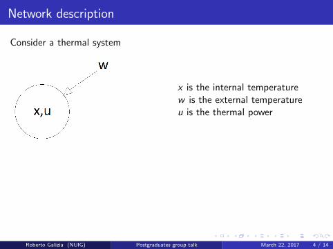
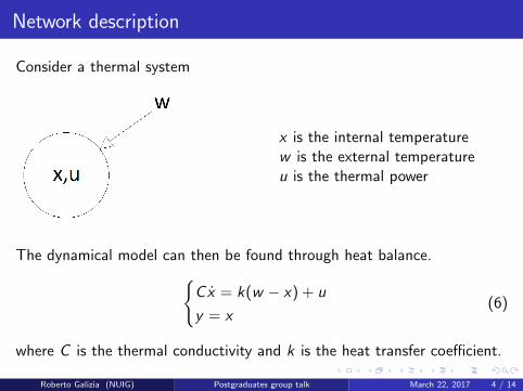
Consider a thermal system
x is the internal temperaturew is the external temperatureu is the thermal power
The dynamical model can then be found through heat balance.{Cx = k(w − x) + u
y = x(6)
where C is the thermal conductivity and k is the heat transfer coefficient.
Roberto Galizia (NUIG) Postgraduates group talk March 22, 2017 4 / 14
Network description
Consider a thermal system
x is the internal temperaturew is the external temperatureu is the thermal power
The dynamical model can then be found through heat balance.{Cx = k(w − x) + u
y = x(6)
where C is the thermal conductivity and k is the heat transfer coefficient.
Roberto Galizia (NUIG) Postgraduates group talk March 22, 2017 4 / 14

Network description
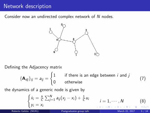
Consider now an undirected complex network of N nodes.
Defining the Adjacency matrix
{Adj}ij = aij =
{1 if there is an edge between i and j
0 otherwise(7)
the dynamics of a generic node is given by{xi = k
C
∑Nj=1 aij(xj − xi ) + 1
C ui
yi = xii = 1, · · · ,N (8)
Roberto Galizia (NUIG) Postgraduates group talk March 22, 2017 5 / 14

Network description
Consider now an undirected complex network of N nodes.
Defining the Adjacency matrix
{Adj}ij = aij =
{1 if there is an edge between i and j
0 otherwise(7)
the dynamics of a generic node is given by{xi = k
C
∑Nj=1 aij(xj − xi ) + 1
C ui
yi = xii = 1, · · · ,N (8)
Roberto Galizia (NUIG) Postgraduates group talk March 22, 2017 5 / 14

Network description
Introducing the Laplacian matrix
{L}ij =
ki if i = j
−1 if i 6= j ∧ there is an edge between i and j
0 otherwise
(9)
where ki is the degree of the node i , i.e. the number of edges connectedto i ,
defining the vectors
x =
x1...xN
u =
u1...uN
y =
y1...yN
(10)
the global differential equation that describes the dynamics of the networkis {
x = − kC Lx + 1
C Iu
y = x(11)
Roberto Galizia (NUIG) Postgraduates group talk March 22, 2017 6 / 14

Network description
Introducing the Laplacian matrix
{L}ij =
ki if i = j
−1 if i 6= j ∧ there is an edge between i and j
0 otherwise
(9)
where ki is the degree of the node i , i.e. the number of edges connectedto i , defining the vectors
x =
x1...xN
u =
u1...uN
y =
y1...yN
(10)
the global differential equation that describes the dynamics of the networkis {
x = − kC Lx + 1
C Iu
y = x(11)
Roberto Galizia (NUIG) Postgraduates group talk March 22, 2017 6 / 14

Centralized control
Given an initial condition
x(0) =[x01 · · · x0N
]T(12)
defining the matrix A and B
A = − kC L ∈ RN×N B = 1
C I ∈ RN×N (13)
the differential equation (11) can be rewritten as
x = Ax + Bu (14)
Assuming that the desired state is constant
xd =[xd1 · · · xdN
]T(15)
we want the state x to converge to xd .
Roberto Galizia (NUIG) Postgraduates group talk March 22, 2017 7 / 14

Centralized control
Let us introduce the error ε = x− xd
ε = x = Ax + Bu = Aε+ Bu + Axd (16)
By choosing a control action
u = u− BT (BBT )−1Axd (17)
the dynamics of the error is given by the linear system
ε = Aε+ Bu (18)
then the choiceu = −Kε (19)
where K is calculated as in (4), minimizes the cost functional
J =
∫ +∞
0εTQε+ uTRu (20)
Roberto Galizia (NUIG) Postgraduates group talk March 22, 2017 8 / 14

Decentralized control
Why decentralize the control?
The centralized controller is optimal and easy to implement but itmust be set by a unique global processor which has knoledge of thewhole network, i.e. it must communicate with all the nodes and mustcalculate online the Laplacian matrix.
If each node has is own processor and it is able to compute its own con-trol action it reasonable to assume that the only available informationsare local, i.e. about the node itself and its neighbours.
The controller is not optimal anymore, but the computation can bespread all over the nodes.
Adding/removing a node does not affect the whole network but only asmall subset of nodes.
Roberto Galizia (NUIG) Postgraduates group talk March 22, 2017 9 / 14

Decentralized control
Assume then that each node is aware only of itself and its neighbourszi = {{xi} ∩ xj∀j : aij = 1},
we have a set of N star sub-networks.
And the model for each node is
xi =k
C
∑j :xj∈zi
(xj − xi ) +1
Cui (21)
Roberto Galizia (NUIG) Postgraduates group talk March 22, 2017 10 / 14

Decentralized control
Assume then that each node is aware only of itself and its neighbourszi = {{xi} ∩ xj∀j : aij = 1}, we have a set of N star sub-networks.
And the model for each node is
xi =k
C
∑j :xj∈zi
(xj − xi ) +1
Cui (21)
Roberto Galizia (NUIG) Postgraduates group talk March 22, 2017 10 / 14

Decentralized control
Considering the Laplacian matrix Li of the i − th sub-network, thedynamics can be rewritten in matrix form as
zi = − k
CLizi +
1
Cbiui (22)
where bi is a vector with one only 1 at the position i and all 0 elsewhere.
Defining the local error εi = {{(xi − xdi )} ∪ (xj − xdj )∀j : aij = 1}Let
Ai = − k
CLi and Bi =
1
Cbi (23)
The control action can be chosen, as the LQR solution of the subnetwork,
ui = −BTi (BiB
Ti )−1Aixdi −Kiεi (24)
whit Ki calculated with (4), minimizing the cost functional
Ji =
∫ +∞
0εTi Qεi + ru2i (25)
Roberto Galizia (NUIG) Postgraduates group talk March 22, 2017 11 / 14

Decentralized control
Considering the Laplacian matrix Li of the i − th sub-network, thedynamics can be rewritten in matrix form as
zi = − k
CLizi +
1
Cbiui (22)
where bi is a vector with one only 1 at the position i and all 0 elsewhere.Defining the local error εi = {{(xi − xdi )} ∪ (xj − xdj )∀j : aij = 1}
Let
Ai = − k
CLi and Bi =
1
Cbi (23)
The control action can be chosen, as the LQR solution of the subnetwork,
ui = −BTi (BiB
Ti )−1Aixdi −Kiεi (24)
whit Ki calculated with (4), minimizing the cost functional
Ji =
∫ +∞
0εTi Qεi + ru2i (25)
Roberto Galizia (NUIG) Postgraduates group talk March 22, 2017 11 / 14

Decentralized control
Considering the Laplacian matrix Li of the i − th sub-network, thedynamics can be rewritten in matrix form as
zi = − k
CLizi +
1
Cbiui (22)
where bi is a vector with one only 1 at the position i and all 0 elsewhere.Defining the local error εi = {{(xi − xdi )} ∪ (xj − xdj )∀j : aij = 1}Let
Ai = − k
CLi and Bi =
1
Cbi (23)
The control action can be chosen, as the LQR solution of the subnetwork,
ui = −BTi (BiB
Ti )−1Aixdi −Kiεi (24)
whit Ki calculated with (4), minimizing the cost functional
Ji =
∫ +∞
0εTi Qεi + ru2i (25)
Roberto Galizia (NUIG) Postgraduates group talk March 22, 2017 11 / 14

Results and comparison
With xdi = 25 ∀i , both the controllers complete the task
and as it was expected, the centralized control performs better
Roberto Galizia (NUIG) Postgraduates group talk March 22, 2017 12 / 14

Results and comparison
With xdi = 25 ∀i , both the controllers complete the task
and as it was expected, the centralized control performs better
Roberto Galizia (NUIG) Postgraduates group talk March 22, 2017 12 / 14

Forthcoming research
What’s next?
Study the stability of the controlled system
Find out which mechanisms can lead to instability
... and moreover
Induce structural changes by varying critical parameters
Generalize the analysis to more complicated systems
Roberto Galizia (NUIG) Postgraduates group talk March 22, 2017 13 / 14

References
Stephen Boyd and Lieven Vandenberghe (2004)
Convex Optimization
University Press, Cambridge
Chao Liu, Zhisheng Duan, Guanrong Chen, and Lin Huang (2009)
L2 norm performance index of synchronization and lqr control synthesis of complexnetworks
Automatica 45(8):18791885
M. Newman (2010)
Networks: An Introduction
OUP Oxford
Roberto Galizia (NUIG) Postgraduates group talk March 22, 2017 14 / 14