university of california

riverside

Search for WZ Production in the Tri-lepton Channel at the

Tevatron and Limits on the WWZ Vertex Anomalous Couplings

A Dissertation submitted in partial satisfaction

of the requirements for the degree of

Doctor of Philosophy

in

Physics

by

Patrick Elmo Gartung

December, 1998

Dissertation Committee:

Dr. John Ellison, Chairperson

Dr. Benjamin Shen

Dr. Stephen Wimpenny

Copyright by

Patrick Elmo Gartung

1998

The Dissertation of Patrick Elmo Gartung is approved:

Committee Chairperson

University of California, Riverside

Acknowledgements

It is traditional at this point to acknowledge those who have helped in the

process of obtaining a Ph.D. There are a great many people who have helped me

over the years and if I have left anyone out my sincerest apologies.

Firstly I would like to thank the D� collaboration. I came in late on the

experiment after the detector had been built and the software written. If it were not

for the e�ort of hundreds of physicists over many years I would not have had any

data to perform my analysis on. I would also like to thank the Fermilab Accelerator

and Computing Divisions whose help was essential in performing the experiment.

I would like to thank my advisor John Ellison for introducing me to the world

of particle physics and giving me an interesting problem to research. Without his

support and lots and lots of patience I would never have �nished.

I would like to thank the members of the U.C. Riverside D� group who

have helped me: Jim Cochran, Chris Boswell, Krish Gounder, Steve Wimpenny and

Ann Heinson. Yvonne Ayers deserves a mention for her help in taking care of the

administrative details for the group.

I would like to thank the people at Fermilab who have helped me. Tom Diehl,

Taka Yasuda, Greg Landsberg, Steve Glenn, Paul Bloom and other members of the

iv

diboson research group helped me understand the business of diboson physics and

limit setting. Dave Buchholz and the members of Editorial Board 110 were crucial

in \fact checking" my �nal numbers. Paul Russo, Scott Snyder and Paul Rubinov

were there for me when I needed someone to talk to.

I would like to thank my friends who made life in graduate school more

bearable: fellow Riverside students Martin Mason, Happy Singh, Christian Minor

and Mike Crivello, and the Friday night crew Jim, Eric, Hayley and Caryn.

I would like to thank my parents for their support and encouragement in

pursuing my education.

Last but not least, I owe a deep debt of gratitude to my wife Julie. Her love

and encouragement were essential in the completion of my research.

v

To

Julie and Baby M

And

My Parents

vi

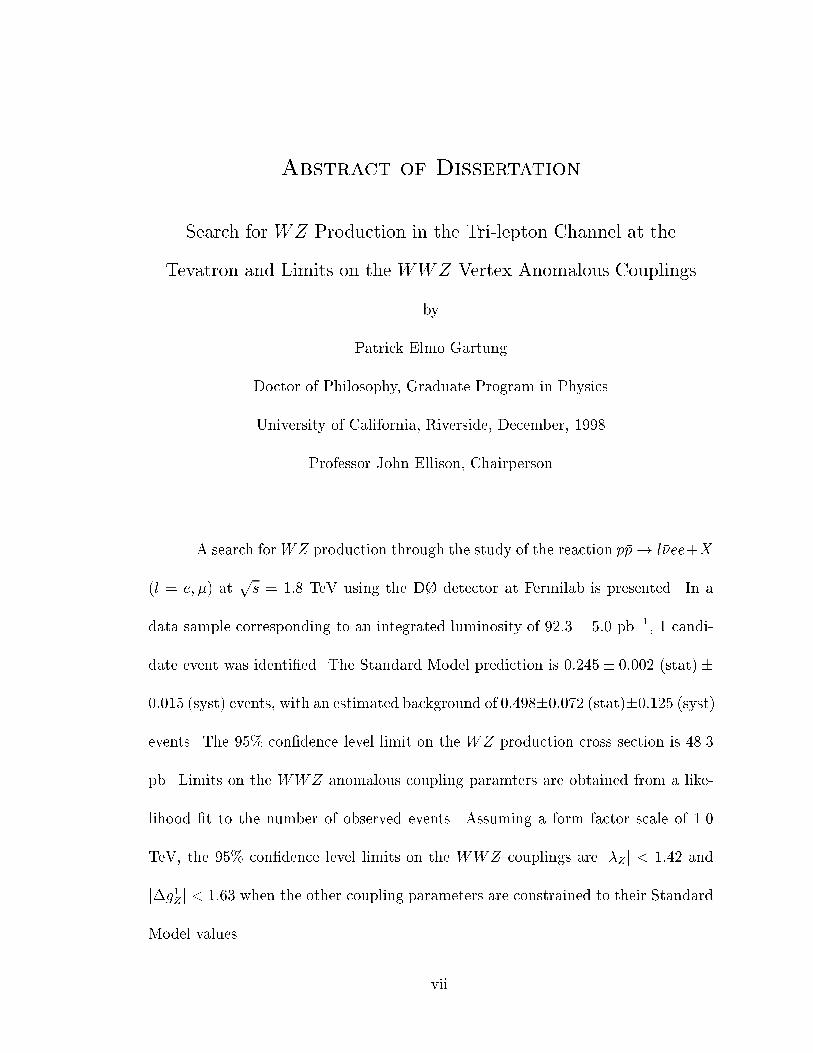
Abstract of Dissertation

Search for WZ Production in the Tri-lepton Channel at the

Tevatron and Limits on the WWZ Vertex Anomalous Couplings

by

Patrick Elmo Gartung

Doctor of Philosophy, Graduate Program in Physics

University of California, Riverside, December, 1998

Professor John Ellison, Chairperson

A search forWZ production through the study of the reaction p�p! l��ee+X

(l = e; �) atps = 1:8 TeV using the D� detector at Fermilab is presented. In a

data sample corresponding to an integrated luminosity of 92:3� 5:0 pb�1, 1 candi-

date event was identi�ed. The Standard Model prediction is 0:245� 0:002 (stat)�

0:015 (syst) events, with an estimated background of 0:498�0:072 (stat)�0:125 (syst)

events. The 95% con�dence level limit on the WZ production cross section is 48.3

pb. Limits on the WWZ anomalous coupling paramters are obtained from a like-

lihood �t to the number of observed events. Assuming a form factor scale of 1.0

TeV, the 95% con�dence level limits on the WWZ couplings are j�Zj < 1:42 and

j�g1Zj < 1:63 when the other coupling parameters are constrained to their Standard

Model values.

vii

Contents

List of Tables x

List of Figures xi

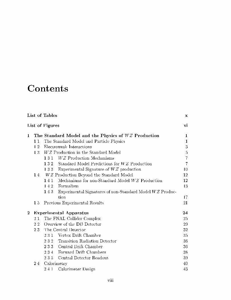
1 The Standard Model and the Physics of WZ Production 1

1.1 The Standard Model and Particle Physics . . . . . . . . . . . . . . . 11.2 Electroweak Interactions . . . . . . . . . . . . . . . . . . . . . . . . . 31.3 WZ Production in the Standard Model . . . . . . . . . . . . . . . . . 5

1.3.1 WZ Production Mechanisms . . . . . . . . . . . . . . . . . . . 71.3.2 Standard Model Predictions for WZ Production . . . . . . . . 71.3.3 Experimental Signature of WZ production . . . . . . . . . . . 10

1.4 WZ Production Beyond the Standard Model . . . . . . . . . . . . . 121.4.1 Mechanisms for non-Standard Model WZ Production . . . . . 121.4.2 Formalism . . . . . . . . . . . . . . . . . . . . . . . . . . . . . 131.4.3 Experimental Signatures of non-Standard ModelWZ Produc-

tion . . . . . . . . . . . . . . . . . . . . . . . . . . . . . . . . 171.5 Previous Experimental Results . . . . . . . . . . . . . . . . . . . . . . 21

2 Experimental Apparatus 24

2.1 The FNAL Collider Complex . . . . . . . . . . . . . . . . . . . . . . 252.2 Overview of the D� Detector . . . . . . . . . . . . . . . . . . . . . . 292.3 The Central Detector . . . . . . . . . . . . . . . . . . . . . . . . . . . 32

2.3.1 Vertex Drift Chamber . . . . . . . . . . . . . . . . . . . . . . 352.3.2 Transition Radiation Detector . . . . . . . . . . . . . . . . . . 362.3.3 Central Drift Chamber . . . . . . . . . . . . . . . . . . . . . . 362.3.4 Forward Drift Chambers . . . . . . . . . . . . . . . . . . . . . 382.3.5 Central Detector Readout . . . . . . . . . . . . . . . . . . . . 39

2.4 Calorimetry . . . . . . . . . . . . . . . . . . . . . . . . . . . . . . . . 402.4.1 Calorimeter Design . . . . . . . . . . . . . . . . . . . . . . . . 43

viii

2.4.2 Central Calorimeter . . . . . . . . . . . . . . . . . . . . . . . . 472.4.3 Endcap Calorimeters . . . . . . . . . . . . . . . . . . . . . . . 482.4.4 Intercryostat Detectors and Massless Gaps . . . . . . . . . . . 502.4.5 Calorimeter Readout . . . . . . . . . . . . . . . . . . . . . . . 502.4.6 Calorimeter Performance . . . . . . . . . . . . . . . . . . . . . 51

2.5 Muon Tracking . . . . . . . . . . . . . . . . . . . . . . . . . . . . . . 522.5.1 WAMUS . . . . . . . . . . . . . . . . . . . . . . . . . . . . . . 522.5.2 SAMUS . . . . . . . . . . . . . . . . . . . . . . . . . . . . . . 54

2.6 Trigger and Data Acquisition . . . . . . . . . . . . . . . . . . . . . . 542.6.1 Level 0 . . . . . . . . . . . . . . . . . . . . . . . . . . . . . . . 562.6.2 Beam Vetoes . . . . . . . . . . . . . . . . . . . . . . . . . . . 562.6.3 Level 1 . . . . . . . . . . . . . . . . . . . . . . . . . . . . . . . 572.6.4 Level 1.5 . . . . . . . . . . . . . . . . . . . . . . . . . . . . . . 582.6.5 Level 2 . . . . . . . . . . . . . . . . . . . . . . . . . . . . . . . 59

2.7 Online Cluster . . . . . . . . . . . . . . . . . . . . . . . . . . . . . . . 602.8 O�ine Data Processing . . . . . . . . . . . . . . . . . . . . . . . . . . 60

3 Event Reconstruction and Particle Identi�cation 62

3.1 Track Reconstruction . . . . . . . . . . . . . . . . . . . . . . . . . . . 633.2 Vertex Finding . . . . . . . . . . . . . . . . . . . . . . . . . . . . . . 633.3 Calorimeter Hit Finding . . . . . . . . . . . . . . . . . . . . . . . . . 643.4 Missing Energy . . . . . . . . . . . . . . . . . . . . . . . . . . . . . . 663.5 Jet Reconstruction . . . . . . . . . . . . . . . . . . . . . . . . . . . . 663.6 Electron{Photon Reconstruction . . . . . . . . . . . . . . . . . . . . . 673.7 Electron Identi�cation . . . . . . . . . . . . . . . . . . . . . . . . . . 69

3.7.1 Electromagnetic Shower Shape Analysis . . . . . . . . . . . . 693.7.2 Shower Isolation . . . . . . . . . . . . . . . . . . . . . . . . . 703.7.3 Track{Cluster Matching . . . . . . . . . . . . . . . . . . . . . 713.7.4 Hit Counting Techniques . . . . . . . . . . . . . . . . . . . . . 72

3.8 Muon Reconstruction . . . . . . . . . . . . . . . . . . . . . . . . . . . 743.9 Muon Identi�cation . . . . . . . . . . . . . . . . . . . . . . . . . . . . 753.10 Post-RECO Corrections . . . . . . . . . . . . . . . . . . . . . . . . . 77

3.10.1 Jet Corrections . . . . . . . . . . . . . . . . . . . . . . . . . . 773.10.2 Revertexing by Cluster-Track Projection . . . . . . . . . . . . 783.10.3 Missing Energy Corrections . . . . . . . . . . . . . . . . . . . 81

4 Event Selection 82

4.1 Data Samples . . . . . . . . . . . . . . . . . . . . . . . . . . . . . . . 824.2 Luminosity . . . . . . . . . . . . . . . . . . . . . . . . . . . . . . . . 834.3 Trigger . . . . . . . . . . . . . . . . . . . . . . . . . . . . . . . . . . . 844.4 O�ine Electron Selection . . . . . . . . . . . . . . . . . . . . . . . . . 85

ix

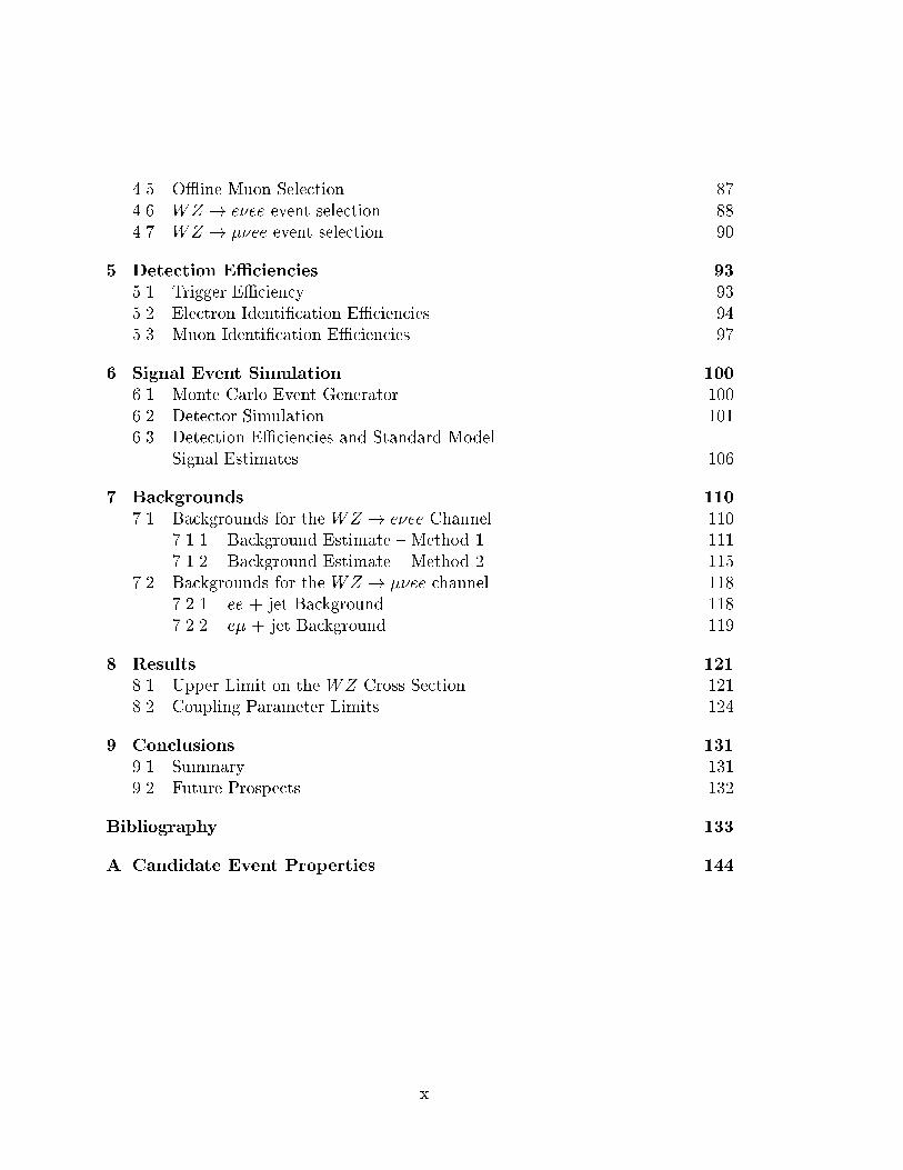
4.5 O�ine Muon Selection . . . . . . . . . . . . . . . . . . . . . . . . . . 874.6 WZ ! e�ee event selection. . . . . . . . . . . . . . . . . . . . . . . . 884.7 WZ ! ��ee event selection . . . . . . . . . . . . . . . . . . . . . . . 90

5 Detection E�ciencies 93

5.1 Trigger E�ciency . . . . . . . . . . . . . . . . . . . . . . . . . . . . . 935.2 Electron Identi�cation E�ciencies . . . . . . . . . . . . . . . . . . . . 945.3 Muon Identi�cation E�ciencies . . . . . . . . . . . . . . . . . . . . . 97

6 Signal Event Simulation 100

6.1 Monte Carlo Event Generator . . . . . . . . . . . . . . . . . . . . . . 1006.2 Detector Simulation . . . . . . . . . . . . . . . . . . . . . . . . . . . . 1016.3 Detection E�ciencies and Standard Model

Signal Estimates . . . . . . . . . . . . . . . . . . . . . . . . . . . . . 106

7 Backgrounds 110

7.1 Backgrounds for the WZ ! e�ee Channel . . . . . . . . . . . . . . . 1107.1.1 Background Estimate { Method 1 . . . . . . . . . . . . . . . . 1117.1.2 Background Estimate { Method 2 . . . . . . . . . . . . . . . . 115

7.2 Backgrounds for the WZ ! ��ee channel . . . . . . . . . . . . . . . 1187.2.1 ee + jet Background . . . . . . . . . . . . . . . . . . . . . . . 1187.2.2 e� + jet Background . . . . . . . . . . . . . . . . . . . . . . . 119

8 Results 121

8.1 Upper Limit on the WZ Cross Section . . . . . . . . . . . . . . . . . 1218.2 Coupling Parameter Limits . . . . . . . . . . . . . . . . . . . . . . . . 124

9 Conclusions 131

9.1 Summary . . . . . . . . . . . . . . . . . . . . . . . . . . . . . . . . . 1319.2 Future Prospects . . . . . . . . . . . . . . . . . . . . . . . . . . . . . 132

Bibliography 133

A Candidate Event Properties 144

x

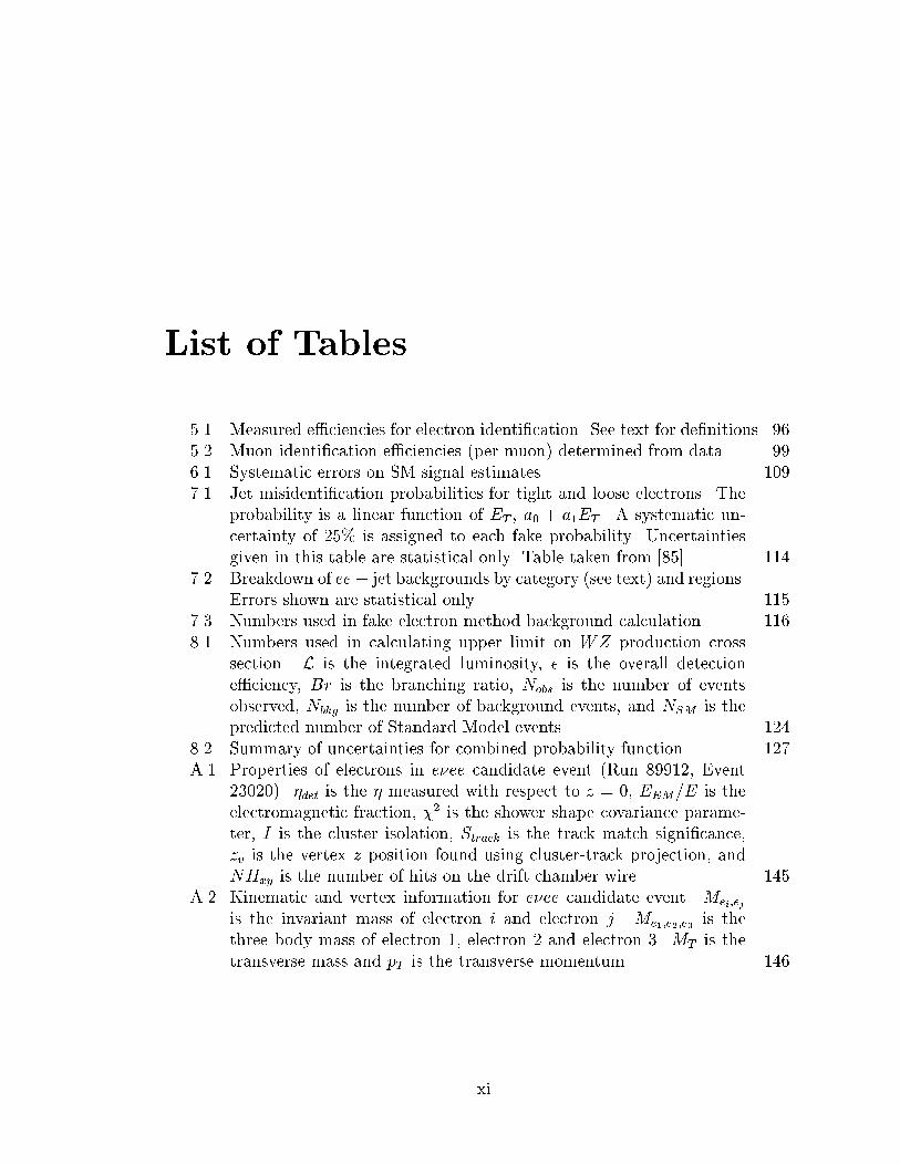
List of Tables

5.1 Measured e�ciencies for electron identi�cation. See text for de�nitions. 965.2 Muon identi�cation e�ciencies (per muon) determined from data. . . 996.1 Systematic errors on SM signal estimates. . . . . . . . . . . . . . . . 1097.1 Jet misidenti�cation probabilities for tight and loose electrons. The

probability is a linear function of ET , a0 + a1ET . A systematic un-certainty of 25% is assigned to each fake probability. Uncertaintiesgiven in this table are statistical only. Table taken from [85]. . . . . . 114

7.2 Breakdown of ee + jet backgrounds by category (see text) and regions.Errors shown are statistical only. . . . . . . . . . . . . . . . . . . . . 115

7.3 Numbers used in fake electron method background calculation. . . . 1168.1 Numbers used in calculating upper limit on WZ production cross

section. L is the integrated luminosity, � is the overall detectione�ciency, Br is the branching ratio, Nobs is the number of eventsobserved, Nbkg is the number of background events, and NSM is thepredicted number of Standard Model events. . . . . . . . . . . . . . . 124

8.2 Summary of uncertainties for combined probability function. . . . . . 127A.1 Properties of electrons in e�ee candidate event (Run 89912, Event

23020). �det is the � measured with respect to z = 0, EEM=E is theelectromagnetic fraction, �2 is the shower shape covariance parame-ter, I is the cluster isolation, Strack is the track match signi�cance,zv is the vertex z position found using cluster-track projection, andNHxy is the number of hits on the drift chamber wire. . . . . . . . . 145

A.2 Kinematic and vertex information for e�ee candidate event. Mei;ej

is the invariant mass of electron i and electron j. Me1;e2;e3 is thethree body mass of electron 1, electron 2 and electron 3. MT is thetransverse mass and pT is the transverse momentum. . . . . . . . . . 146

xi

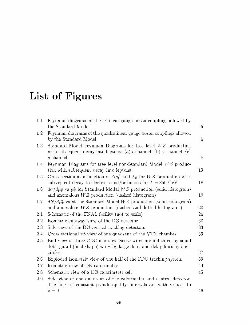
List of Figures

1.1 Feynman diagrams of the trilinear gauge boson couplings allowed bythe Standard Model. . . . . . . . . . . . . . . . . . . . . . . . . . . . 5

1.2 Feynman diagrams of the quadralinear gauge boson couplings allowedby the Standard Model. . . . . . . . . . . . . . . . . . . . . . . . . . 6

1.3 Standard Model Feynman Diagrams for tree level WZ productionwith subsequent decay into leptons: (a) t-channel; (b) u-channel; (c)s-channel. . . . . . . . . . . . . . . . . . . . . . . . . . . . . . . . . . 8

1.4 Feynman Diagrams for tree level non-Standard Model WZ produc-tion with subsequent decay into leptons. . . . . . . . . . . . . . . . . 13

1.5 Cross section as a function of �gZ1 and �Z for WZ production withsubsequent decay to electrons and/or muons for � = 850 GeV. . . . . 18

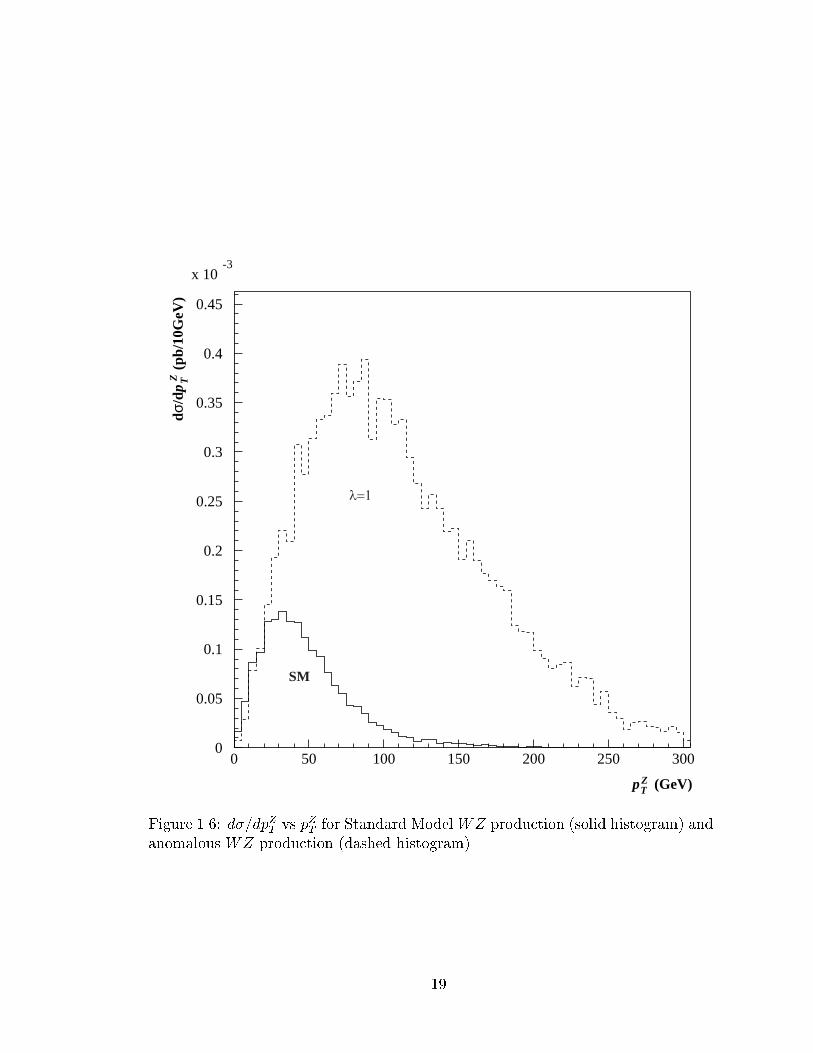
1.6 d�=dpZT vs pZT for Standard Model WZ production (solid histogram)and anomalous WZ production (dashed histogram). . . . . . . . . . . 19

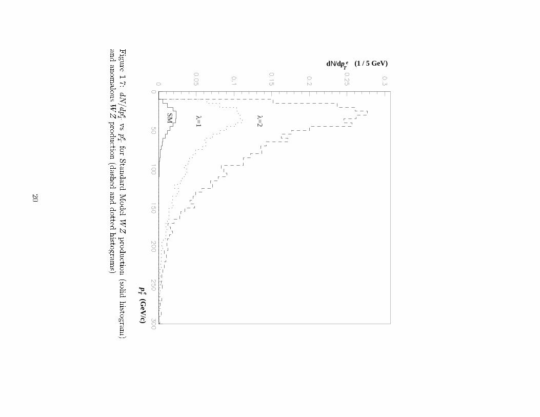
1.7 dN=dpeT vs peT for Standard Model WZ production (solid histogram)and anomalous WZ production (dashed and dotted histograms). . . . 20

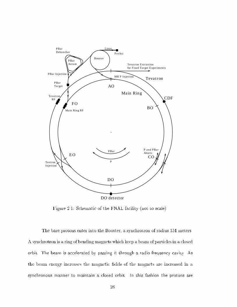
2.1 Schematic of the FNAL facility (not to scale). . . . . . . . . . . . . . 26

2.2 Isometric cutaway view of the D� detector. . . . . . . . . . . . . . . 30

2.3 Side view of the D� central tracking detectors. . . . . . . . . . . . . . 33

2.4 Cross sectional r� view of one quadrant of the VTX chamber. . . . . 35

2.5 End view of three CDC modules. Sense wires are indicated by smalldots, guard (�eld shape) wires by large dots, and delay lines by opencircles. . . . . . . . . . . . . . . . . . . . . . . . . . . . . . . . . . . . 37

2.6 Exploded isometric view of one half of the FDC tracking system. . . . 39

2.7 Isometric view of D� calorimetry. . . . . . . . . . . . . . . . . . . . . 44

2.8 Schematic view of a D� calorimeter cell. . . . . . . . . . . . . . . . . 45

2.9 Side view of one quadrant of the calorimeter and central detector.The lines of constant pseudorapidity intervals are with respect toz = 0. . . . . . . . . . . . . . . . . . . . . . . . . . . . . . . . . . . . 46

xii

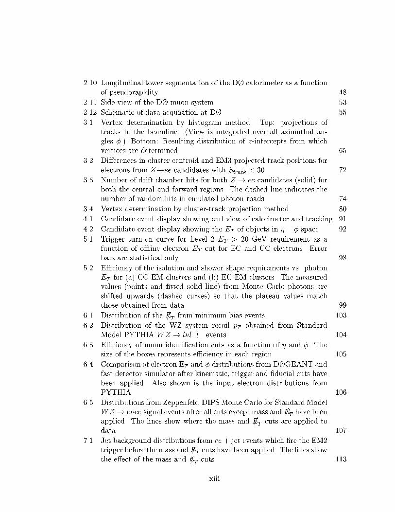
2.10 Longitudinal tower segmentation of the D� calorimeter as a functionof pseudorapidity. . . . . . . . . . . . . . . . . . . . . . . . . . . . . . 48

2.11 Side view of the D� muon system. . . . . . . . . . . . . . . . . . . . 53

2.12 Schematic of data acquisition at D�. . . . . . . . . . . . . . . . . . . 55

3.1 Vertex determination by histogram method. Top: projections oftracks to the beamline. (View is integrated over all azimuthal an-gles �.) Bottom: Resulting distribution of z-intercepts from whichvertices are determined. . . . . . . . . . . . . . . . . . . . . . . . . . 65

3.2 Di�erences in cluster centroid and EM3 projected track positions forelectrons from Z!ee candidates with Strack < 30. . . . . . . . . . . . 72

3.3 Number of drift chamber hits for both Z ! ee candidates (solid) forboth the central and forward regions. The dashed line indicates thenumber of random hits in emulated photon roads. . . . . . . . . . . . 74

3.4 Vertex determination by cluster-track projection method. . . . . . . . 80

4.1 Candidate event display showing end view of calorimeter and tracking. 91

4.2 Candidate event display showing the ET of objects in � � � space. . . 92

5.1 Trigger turn-on curve for Level 2 ET > 20 GeV requirement as afunction of o�ine electron ET cut for EC and CC electrons. Errorbars are statistical only. . . . . . . . . . . . . . . . . . . . . . . . . . 98

5.2 E�ciency of the isolation and shower shape requirements vs. photonET for (a) CC EM clusters and (b) EC EM clusters. The measuredvalues (points and �tted solid line) from Monte Carlo photons areshifted upwards (dashed curves) so that the plateau values matchthose obtained from data. . . . . . . . . . . . . . . . . . . . . . . . . 99

6.1 Distribution of the E/T from minimum bias events. . . . . . . . . . . . 103

6.2 Distribution of the WZ system recoil pT obtained from StandardModel PYTHIA WZ ! l�l+l� events. . . . . . . . . . . . . . . . . . 104

6.3 E�ciency of muon identi�cation cuts as a function of � and �. Thesize of the boxes represents e�ciency in each region. . . . . . . . . . . 105

6.4 Comparison of electron ET and � distributions from D�GEANT andfast detector simulator after kinematic, trigger and �ducial cuts havebeen applied. Also shown is the input electron distributions fromPYTHIA. . . . . . . . . . . . . . . . . . . . . . . . . . . . . . . . . . 106

6.5 Distributions from Zeppenfeld-DIPS Monte Carlo for Standard ModelWZ ! e�ee signal events after all cuts except mass and E/T have beenapplied. The lines show where the mass and E/T cuts are applied todata. . . . . . . . . . . . . . . . . . . . . . . . . . . . . . . . . . . . . 107

7.1 Jet background distributions from ee + jet events which �re the EM2trigger before the mass and E/T cuts have been applied. The lines showthe e�ect of the mass and E/T cuts. . . . . . . . . . . . . . . . . . . . 113

xiii

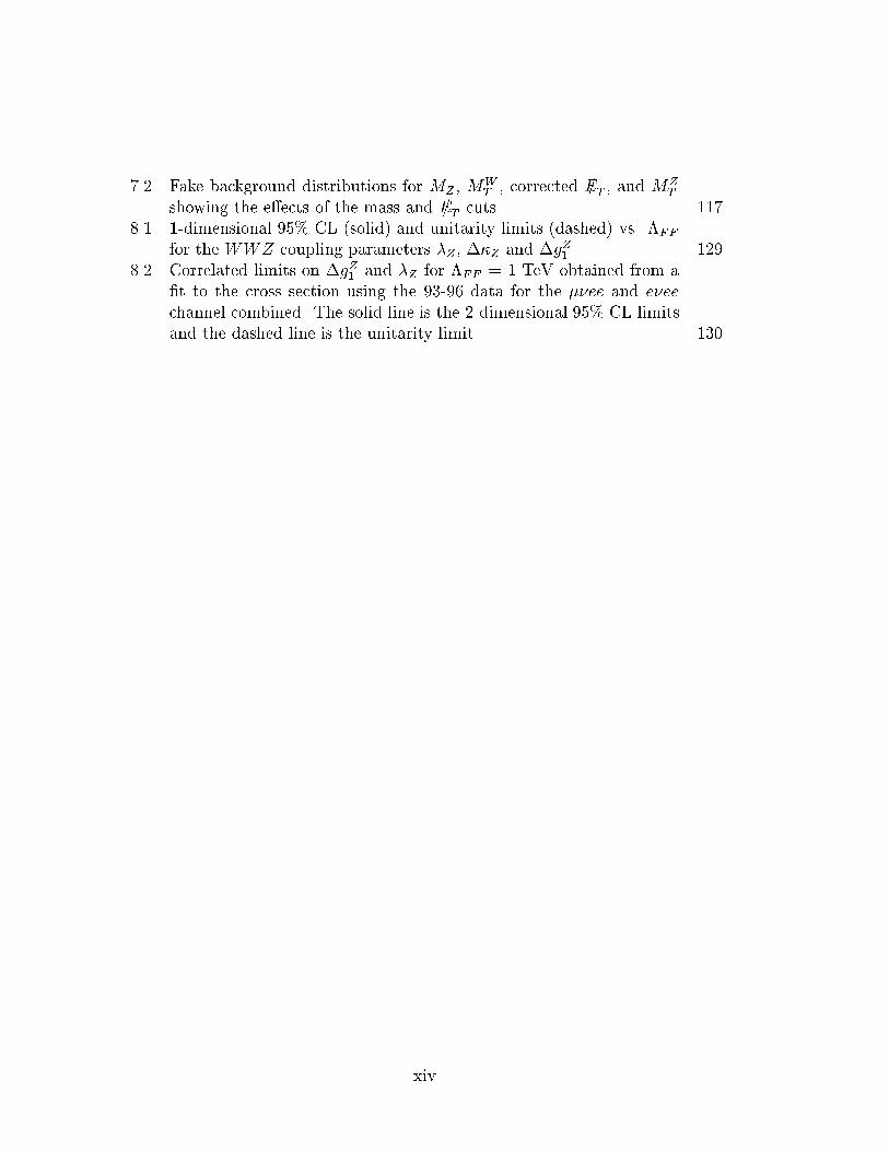
7.2 Fake background distributions for MZ , MWT , corrected E/T , and MZ

T

showing the e�ects of the mass and E/T cuts. . . . . . . . . . . . . . 1178.1 1-dimensional 95% CL (solid) and unitarity limits (dashed) vs. �FF

for the WWZ coupling parameters �Z , ��Z and �gZ1 . . . . . . . . . 1298.2 Correlated limits on �gZ1 and �Z for �FF = 1 TeV obtained from a

�t to the cross section using the 93-96 data for the ��ee and e�eechannel combined. The solid line is the 2-dimensional 95% CL limitsand the dashed line is the unitarity limit. . . . . . . . . . . . . . . . . 130

xiv

Chapter 1

The Standard Model and the

Physics of WZ Production

1.1 The Standard Model and Particle Physics

Over the last 100 years the �eld of particle physics has developed through

the e�orts of experimentalists and theorists. The goal of particle physics is to

develop and test models of the fundamental constituents of matter and the forces

that act between them. One such model has emerged which has been very successful

at explaining experimental data and making predictions for the existence of new

particles. This model has been dubbed the \Standard Model" of particle physics

because of this success.

In the Standard Model, all matter is made up of point-like particles called

1

quarks and leptons. For each particle there is an anti-particle with the same mass

but opposite electric charge. The forces between particles are mediated by the

exchange of bosons. Three of the four fundamental forces of nature are described by

the model: electromagnetism, the \weak" force and the \strong" force. The fourth

force, gravity, is many orders of magnitude weaker than the others at the distance

and energy scales available in the laboratory and can be safely ignored.

Leptons include the familiar electron and its heavier, unstable analogs the

muon and tau, all of which carry charge �1. For each lepton there exists a corre-

sponding neutral particle called a neutrino which has negligible or zero mass.

There are six types of quarks: \up", \down", \strange", \charm", \bottom"

and \top"1. Quarks have the curious property of having fractional electric charge,

+2=3 for up, strange and top, and �1=3 for down, charm, and bottom. Quarks only

exists in pairs or triplets, giving the composite particles a �1 or 0 electric charge.

Quarks also carry color charge, which is associated with the strong force. This is

analogous to the association of the electric charge with the electromagnetic force.

Quarks are the constituents of hadrons. Hadrons include the familiar proton

and neutron and other heavier, unstable particles such as the pion. The proton

is composed of two up quarks and a down quark which are bound together by the

strong force. Through the process of hadronization, a bare quark will bind with other

quarks to form a hadron. A quark would therefore appear as a \jet" of hadrons.

1Conclusive evidence of the existence of the top quark was only recently discovered [1, 2].

2

Leptons and quarks are collectively called fermions. They are so named

because they carry odd half-integer intrinsic angular momentum (spin) and obey

the Pauli exclusion principle of Fermi-Dirac statistics.

Gauge bosons are spin-1 particles which are the carriers of the electromag-

netic, weak and strong forces. They mediate the interactions between quarks and

leptons. The massless photon carries the electromagnetic force over in�nite dis-

tances. The gluons transmit the strong force over a range of order 1 fm, and the

massive W� and Z bosons transmit the weak force over much shorter distances.

In the Standard Model the electromagnetic and weak interactions are uni�ed

into the electroweak force. The focus of this thesis is a test of the predictions of the

electroweak interaction. The electroweak sector of the Standard Model is discussed

in the next section as a basis for further discussion.

1.2 Electroweak Interactions

The SU(2)L � U(1)Y symmetry group is the basis of the Standard Model

of electroweak interactions [3, 4]. In constructing the theory, four gauge �elds are

introduced: W i� (i = 1; 2; 3) for SU(2)L and B� for U(1)Y . The fermions are

written as left- and right-handed �elds, which interact with these gauge �elds. The

3

left-handed fermion �elds are written as isospin doublets

0BBB@

�L

lL

1CCCA

which transform under the j = 1=2 representation of SU(2). The right-handed �elds

are isospin singlets, lR, which transform under the j = 0 (trivial) representation of

SU(2).

The non-Abelian SU(2) group is associated with weak-isospin (I). The

Abelian group U(1)Y is associated with the weak hypercharge, Y . The weak hyper-

charge is related to the electric charge (Q) and the weak-isospin by the Gell-Mann-

Nishijima relation: Q = I3 + Y=2 (I3 is the 3-projection of I).

To give the gauge bosons mass, an isospin doublet of complex scalar Higgs

�elds � is introduced, with a potential function which results in a non-zero vacuum

expectation value for �. This results in the spontaneous breaking of the local SU(2)

gauge symmetry generating masses for the gauge bosons. Of the four �elds only one

corresponds to a physical particle, the Higgs boson [5]. The mass of the Higgs boson

is a free parameter that has not been experimentally measured to date. Indeed,

searching for the Higgs boson and experimental elucidation of the mechanism of

electroweak symmetry breaking is one of the main goals in particle physics.

The electroweak bosons are combinations the the W and B �elds. Linear

combinations of the W1 and W2 �elds are identi�ed as the W� �elds, and linear

combinations of the W3 and B �elds is identi�ed as the Z �eld and the photon

4

�eld, A.

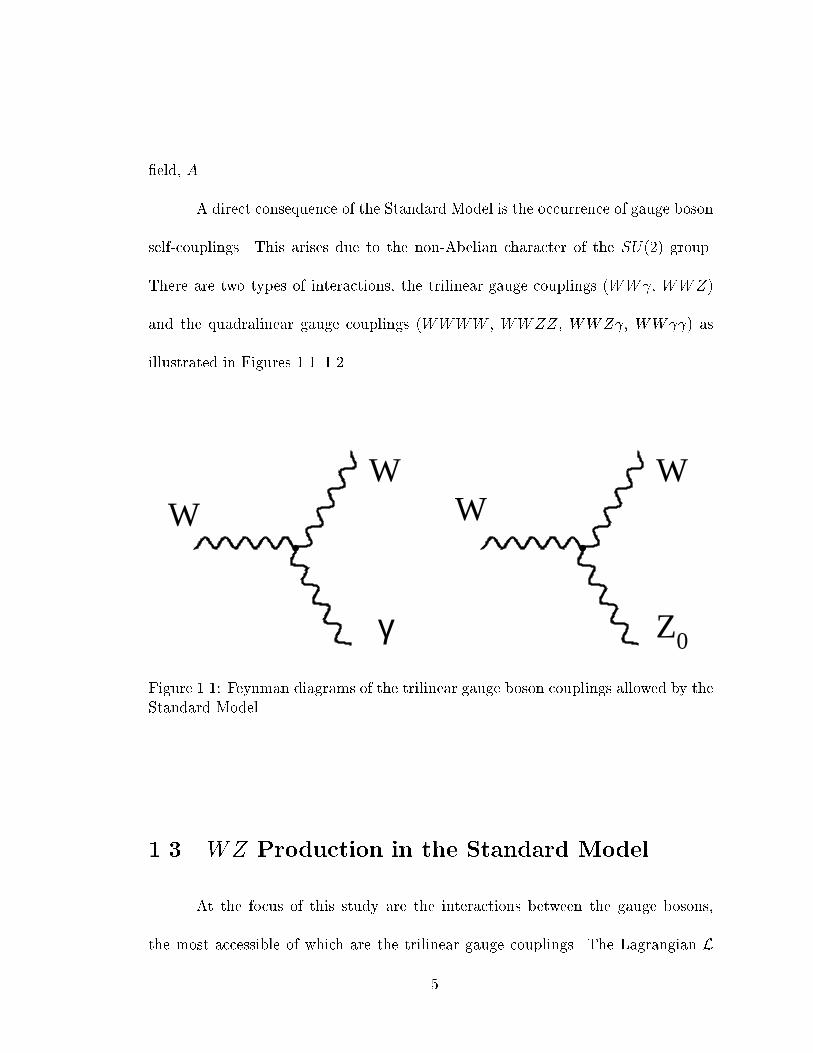
A direct consequence of the Standard Model is the occurrence of gauge boson

self-couplings. This arises due to the non-Abelian character of the SU(2) group.

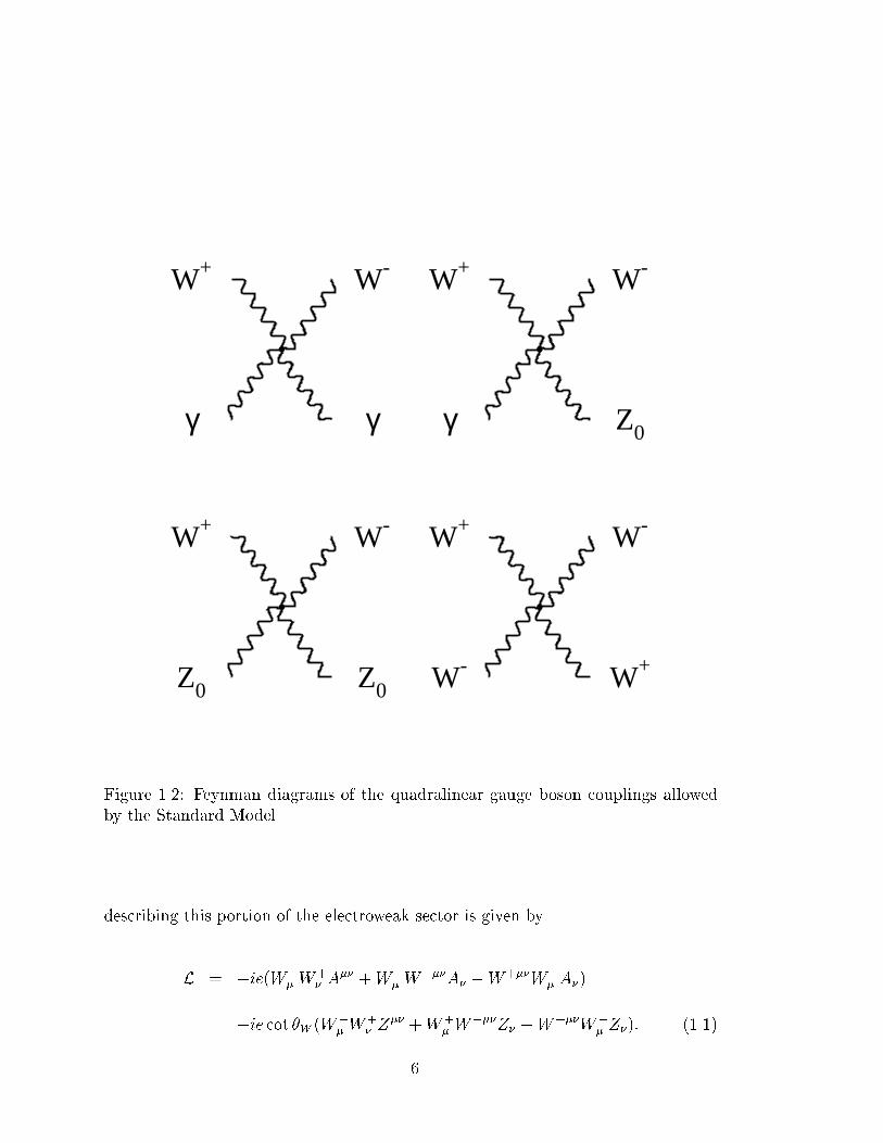
There are two types of interactions, the trilinear gauge couplings (WW , WWZ)

and the quadralinear gauge couplings (WWWW , WWZZ, WWZ , WW ) as

illustrated in Figures 1.1{1.2.

WW

γ

WW

Z0

Figure 1.1: Feynman diagrams of the trilinear gauge boson couplings allowed by theStandard Model.

1.3 WZ Production in the Standard Model

At the focus of this study are the interactions between the gauge bosons,

the most accessible of which are the trilinear gauge couplings. The Lagrangian L

5

W+ W-

γ γ

W+ W-

γ Z0

W+ W-

Z0 Z0

W+ W-

W- W+

Figure 1.2: Feynman diagrams of the quadralinear gauge boson couplings allowedby the Standard Model.

describing this portion of the electroweak sector is given by

L = �ie(W�� W

+� A

�� +W+� W

���A� �W+��W�� A�)

�ie cot �W (W�� W

+� Z

�� +W+� W

���Z� �W+��W�� Z�): (1.1)

6

where �W is the weak mixing angle, W�� is the W� �eld, Z� is the Z �eld, and

A� is the photon �eld. These terms, which specify the WW and WWZ vertices

respectively, arise due to the non-Abelian gauge structure of the electroweak theory.

When combined with the terms describing the fermion couplings to the bosons, these

terms completely describe WZ production at tree level in the Standard Model.

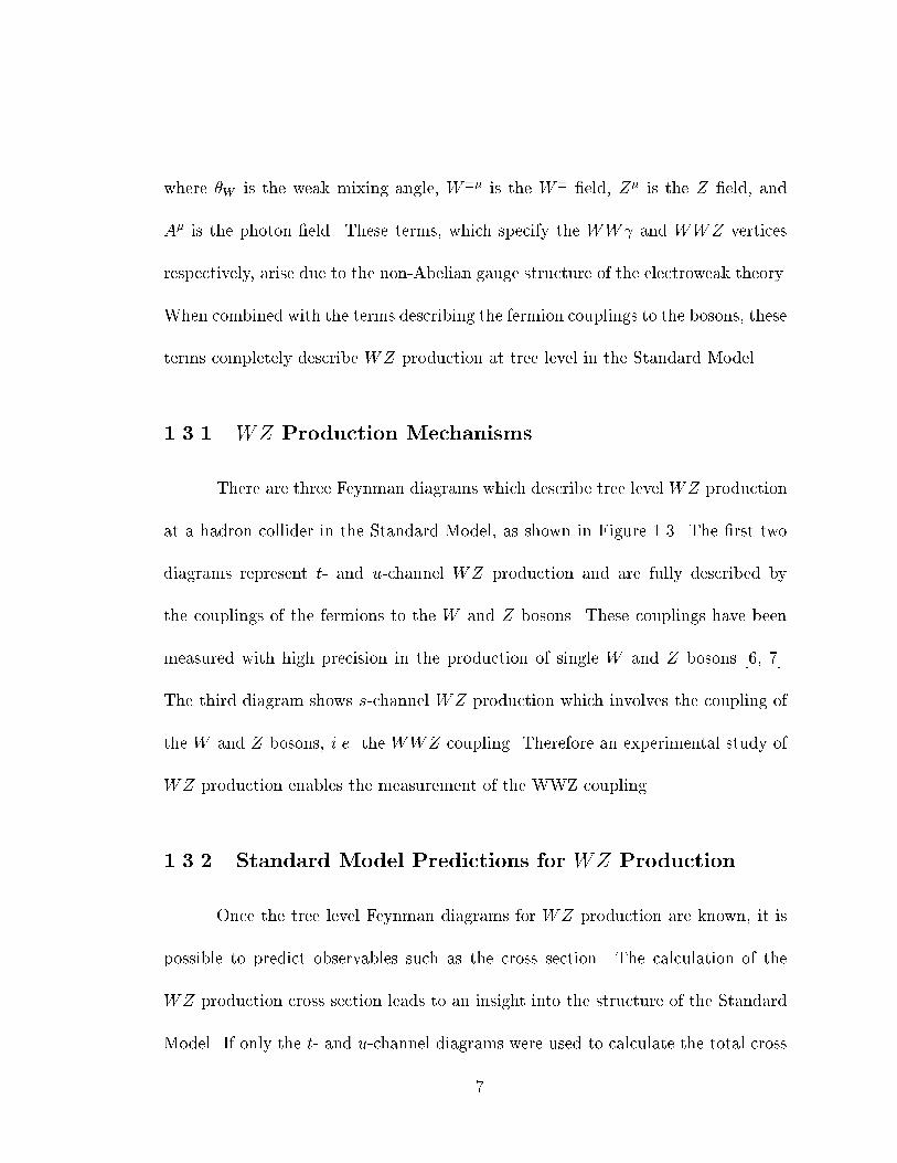
1.3.1 WZ Production Mechanisms

There are three Feynman diagrams which describe tree level WZ production

at a hadron collider in the Standard Model, as shown in Figure 1.3. The �rst two

diagrams represent t- and u-channel WZ production and are fully described by

the couplings of the fermions to the W and Z bosons. These couplings have been

measured with high precision in the production of single W and Z bosons [6, 7].

The third diagram shows s-channel WZ production which involves the coupling of

the W and Z bosons, i.e. the WWZ coupling. Therefore an experimental study of

WZ production enables the measurement of the WWZ coupling.

1.3.2 Standard Model Predictions for WZ Production

Once the tree level Feynman diagrams for WZ production are known, it is

possible to predict observables such as the cross section. The calculation of the

WZ production cross section leads to an insight into the structure of the Standard

Model. If only the t- and u-channel diagrams were used to calculate the total cross

7

q

q´l

νlW

Z

l+

l-

(a)q

q´ l+

l-Z

Wl

νl

(b)

q

q´

l+

l-

l

νlW

Z

W

(c)

Figure 1.3: Standard Model Feynman Diagrams for tree level WZ production withsubsequent decay into leptons: (a) t-channel; (b) u-channel; (c) s-channel.

section, the result would be a linear rise of the cross section with increasingps (the

parton center of mass energy). This implies that for su�ciently large energies partial

wave unitarity will be violated, i.e. the sum of the probabilities of the partial waves

8

will be greater than one. By including the s-channel diagram, which involves the

boson-boson couplings, the cross terms which result from squaring all the summed

amplitudes provide the \delicate" gauge cancellations which are required to restore

unitarity. By construction, the Standard Model provides the gauge boson self-

interaction terms which restore the physical consistency of the model, although these

terms are unnecessary to describe many weak current interactions, such as � decay.

As will be shown later, this cancellation will have important consequences in the

search for deviations from the Standard Model-predicted values for the boson-boson

couplings.

A numerical result for the WZ production cross section cannot be produced

analytically because of the composite nature of the proton and antiproton. The

parton subprocess cross section can be computed analytically, but this must be

summed over all possible pairs of participating partons in the proton and anti-

proton, and additionally integrated over the parton momentum distributions. A

Monte Carlo approach can be used to solve this problem. Event generators such as

PYTHIA [8] can be used to fully model Standard Model WZ production and can

be used to produce a numerical result for the cross section. Another Monte Carlo

provided by the authors of reference [9] uses a fast Monte Carlo approach to model

WZ production. Using the MRSD�0 parton distribution function set [10], the fast

Monte Carlo predicts a Standard Model cross section of 2.6 pb after multiplying the

tree level cross section by a \k-factor" to account for initial and �nal state radiation.

9

Monte Carlo programs can also be used to model the kinematic characteristics of

WZ events.

1.3.3 Experimental Signature of WZ production

WZ production can occur in three distinct channels: those in which both

bosons decay hadronically, those in which one decays hadronically and the other

leptonically, and those in which both decay leptonically.

The purely hadronic �nal state has one advantage. It has as a signi�cantly

larger branching fraction than all leptonic decays. However the disadvantages far

outweigh this advantage. First, it is nearly impossible to reconstruct which hadronic

jet came from which boson. This is due to the �nite energy resolution of hadronic

calorimeters and to the di�culty of the charge sign determination of jets. Further,

the limited energy resolution of hadronic calorimeters makes distinguishingW 's from

Z's di�cult at best. WW and WZ production are therefore indistinguishable in

this channel. Finally this channel su�ers from a large background due to continuum

multijet production as well as the production of singleW or Z bosons in association

with jets.

The semi-leptonic decay modes have the next largest branching fractions,

15% for the l�jj �nal state and 4.5% for the lljj �nal state, where l is an electron

or muon and j is a hadron jet. This channel su�ers from large QCD backgrounds

from both multijet production and W production in association with jets, which is

10

indistinguishable from Standard Model WZ production. As in the fully hadronic

channel, it is impossible to distinguish WZ production from WW production in

the l�jj channel. The lljj �nal state has the advantage of being identi�ed only

with WZ production. However, this �nal state is dominated by backgrounds from

Z production in association with jets. The main advantages of this channel are

the relatively large branching fraction and the ability to unambiguously reconstruct

the momentum of each boson. A cross section measurement in the semi-leptonic

channel is insensitive due the inability to distinguish signal from background.

The purely leptonic �nal state has the smallest branching fraction of all,

1.5% when both electrons and muons are counted (tau's are excluded due to the

di�culty in identifying them e�ciently). The one drawback of this channel is the

relatively small branching fraction. The main advantage of this channel is its unique

signature, three charged leptons with high transverse momentum (pT ), and large

missing transverse energy (E/T ). This signature is unique amongst diboson �nal

states and virtually background free. No physics processes produce a signi�cant

background. The only backgrounds are instrumental backgrounds, which arise from

the misidenti�cation of a jet as a lepton.

As a result of these factors, WZ production in the purely leptonic decay

mode provides a sensitive measure of the cross section and a direct measure of the

WWZ vertex. The search for WZ production in the purely leptonic �nal state is

the subject of this thesis.

11

1.4 WZ Production Beyond the Standard Model

Despite its agreement with all observations to date, it is widely believed that

the Standard Model represents only the low-energy limit of a more fundamental

theory. There are features of the theory which remain unsatisfactory. The required

�ne tuning of quadratic divergences, the \mass hierarchy" issue [11], and the ansatz

nature of the Higgs �eld motivate the search for a more comprehensive theory. At

the energies accessible at today's experiments, de�ciencies in the Standard Model

may only become evident through precision measurements. Deviations in theWWZ

coupling due to non-Standard Model physics will have an e�ect on WZ production.

In this section, the possible mechanisms for non-Standard Model WZ production

are discussed. Following this, a generalized formalism is introduced to cope with

all such scenarios without regard to the details of the particular underlying theory.

Finally, the experimental signature of \anomalous" WZ production is discussed.

1.4.1 Mechanisms for non-Standard Model WZ Production

Many scenarios for physics beyond the Standard Model, which give rise to

non-Standard Model diboson production, have been considered [12, 13, 14, 15, 16,

17, 18, 19, 20, 21, 22]. Most deviations from the Standard Model involve radiative

loop corrections to the trilinear gauge boson vertices. These deviations have been

studied extensively for the WW coupling. Loop corrections involving Standard

12

Model and Supersymmetric particles produce deviations in �� on the order of

10�3 [23]. Other models produce smaller deviations.

1.4.2 Formalism

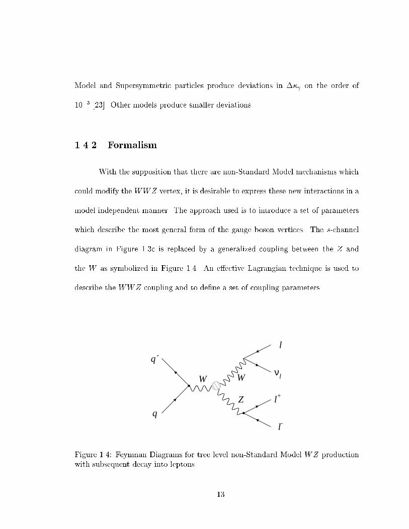
With the supposition that there are non-Standard Model mechanisms which

could modify the WWZ vertex, it is desirable to express these new interactions in a

model independent manner. The approach used is to introduce a set of parameters

which describe the most general form of the gauge boson vertices. The s-channel

diagram in Figure 1.3c is replaced by a generalized coupling between the Z and

the W as symbolized in Figure 1.4. An e�ective Lagrangian technique is used to

describe the WWZ coupling and to de�ne a set of coupling parameters.

q

q´

l+

l-

νl

l

W

Z

W

Figure 1.4: Feynman Diagrams for tree level non-Standard Model WZ productionwith subsequent decay into leptons.

13

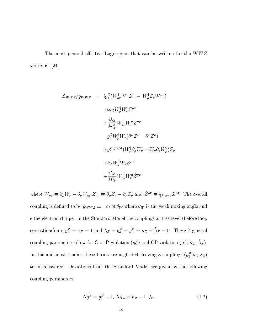
The most general e�ective Lagrangian that can be written for the WWZ

vertex is [24]

LWWZ=gWWZ = igZ1 (Wy��W

�Z� � W y�Z�W

��)

+i�ZWy�W�Z

��

+i�ZM2

W

W y��W

�� Z

��

�gZ4 W y�W�(@

�Z� + @�Z�)

+gZ5 �����(W y

�@�W� �W�@�Wy�)Z�

+~�ZWy�W�

~Z��

+i~�ZM2

W

W y��W

��~Z��

where W�� � @�W� � @�W�, Z�� � @�Z� � @�Z� and ~Z�� � 12�����Z

��. The overall

coupling is de�ned to be gWWZ � �e cot �W where �W is the weak mixing angle and

e the electron charge. In the Standard Model the couplings at tree level (before loop

corrections) are gZ1 = �Z = 1 and �Z = gZ4 = gZ5 = ~�Z = ~�Z = 0. These 7 general

coupling parameters allow for C or P violation (gZ5 ) and CP violation (gZ4 , ~�Z ,~�Z).

In this and most studies these terms are neglected, leaving 3 couplings (gZ1 ,�Z ,�Z)

to be measured. Deviations from the Standard Model are given by the following

coupling parameters:

�gZ1 � gZ1 � 1; ��Z � �Z � 1; �Z (1.2)

14

Other studies, which are sensitive to both the WWZ and WW couplings,

have customarily made assumptions about the relations between the WWZ and

WW coupling parameters. Although a measurement of WZ production is a di-

rect measure of the WWZ vertex coupling parameters it is useful to relate these

parameters to the coupling parameters for the WW vertex for comparison with

other diboson studies. This is accomplished using two di�erent schemes. In the

\equal couplings" scheme the WWZ and WW couplings are assumed to vary by

the same amount. Because �g 1 � 1 by electromagnetic invariance, �gZ1 is �xed at

1, leaving two free parameters: � = �Z = � and �� = ��Z = �� . In the HISZ

scheme [25], the couplings are formulated in a framework which explicitly respects

SU(2)� U(1) gauge invariance. In this scheme the WWZ coupling parameters are

related to the WW parameters by:

�gZ1 =1

2 cos2 �W�� (1.3)

��Z =1

2(1� tan2 �W )�� (1.4)

�Z = � (1.5)

For WZ production the scattering amplitude, M�Z�W , for a Z boson of

helicity �Z and a W boson of helicity �W is enhanced for anomalous couplings. The

M�;� helicity amplitudes are enhanced by s=m2W for anomalous values of �Z and

the M0;0 amplitude is similarly enhanced for �gZ1 . Non-Standard Model values of

15

��Z e�ectM�;0 andM0;�, but only likeps=mW

2. Thus the non-Standard Model

amplitudes rise without limits as s increases and violate partial wave unitarity.

Since the anomalous contribution appears only in the s-channel process, the

l = 0 term in the partial wave expansion must be explicitly controlled. To control

the high energy behavior of the scattering amplitudes, the coupling parameters are

modi�ed by form factors, i.e.

�! �(s) = �=(1 +s

�2)n: (1.6)

For WWZ couplings, the choice of n = 2 is su�cient to bring the high energy

behavior under control. The parameter � is the form factor scale.

For a particular choice of scale �, the unitarity requirement places constraints

on the allowed values of the couplings [26]. If only one coupling parameter at a time

is allowed to vary, the couplings are bounded by

j�gZ1 j � 3:36 TeV2

�2(1.7)

j�Z j � 2:08 TeV2

�2(1.8)

j��Z j � 3:32 TeV2

�2(1.9)

2In fact all diboson processes show a s=m2

Wenhancement for anomalous �. For �gZ

1however,

it is only WZ production which grows as s. For �� only WW production grows linearly with s.Thus WZ production is most sensitive to �gZ

1while WW production is most sensitive to ��.

16

1.4.3 Experimental Signatures of non-Standard Model WZ

Production

Anomalous couplings can be detected by their in uence on observables. The

�rst is a dramatic increase in cross section. Recall from Section 1.3.2 that the

s-channel diagram is required at its Standard Model strength to produce the \deli-

cate" gauge cancellation which controlsWZ production. The presence of anomalous

couplings changes those values and disrupts the cancellation. The larger the devi-

ation from the Standard Model, the larger the disruption. The result is that for

anomalous couplings the cross section is greatly increased (see Fig. 1.5).

In addition to the total cross section, the di�erential distributions are also

sensitive to non-Standard Model couplings. For large values of WZ invariant mass,

the anomalous contributions to the helicity amplitudes dominate the Standard

Model contributions. Because the anomalous contributions come only in the s-

channel, their a�ects tend to be concentrated in regions of small boson rapidity.

Thus the transverse momentum of the bosons and their decay products is enhanced

by the presence of anomalous couplings, particularly at large transverse momen-

tum [27]. Figure 1.6 shows the distribution of pZT for Standard Model and anomalous

couplings and Figure 1.7 shows the pT distribution of the electron from the W for

Standard Model and anomalous couplings.

17

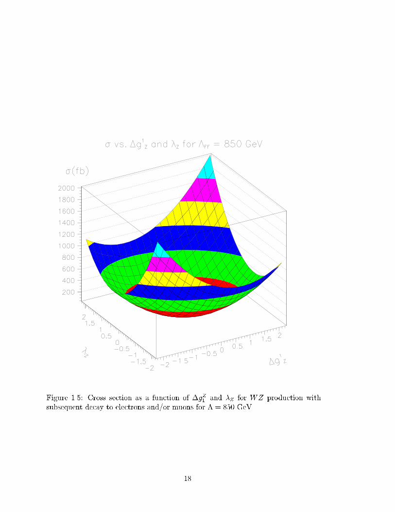
Figure 1.5: Cross section as a function of �gZ1 and �Z for WZ production withsubsequent decay to electrons and/or muons for � = 850 GeV.

18

0

0.05

0.1

0.15

0.2

0.25

0.3

0.35

0.4

0.45

x 10-3

0 50 100 150 200 250 300

pTZ (GeV)

dσ/d

p TZ(p

b/10

GeV

)

SM

Figure 1.6: d�=dpZT vs pZT for Standard ModelWZ production (solid histogram) andanomalous WZ production (dashed histogram).

19

dΝ/dpTe (1 / 5 GeV)

pT e

(GeV

/c)

SM =

1

=2

Figu

re1.7:

dN=dpeTvspeTfor

Stan

dard

ModelWZ

production

(solidhistogram

)andanom

alousWZproduction

(dash

edanddotted

histogram

s).

20

1.5 Previous Experimental Results

Limits can be placed on the coupling parameters by performing a likelihood

test on the measured cross section or kinematic distributions, such as the boson

transverse momentum. To put the results of this analysis in context, the limits on

anomalous couplings obtained from other diboson analyses are presented.

The WW couplings were �rst measured at the UA2 experiment at CERN

to be [28]

�4:5 < �� < 4:9(� = 0) � 3:6 < � < 3:5(�� = 0)

At the Tevatron, CDF reported limits obtained from 20 pb�1 of data of [29]

�2:3 < �� < 2:2(� = 0) � 0:7 < � < 0:7(�� = 0)

while D� derived limits of [30]

�0:93 < �� < 0:94(� = 0) � 0:31 < � < 0:29(�� = 0)

from a full data set of approximately 93 pb�1. The Tevatron limits are obtained

assuming a form factor scale of 1.5 TeV.

Measurements of the WW and WWZ couplings have been made through

WW andWZ �nal states. The limits are quoted assuming the \equal couplings" sce-

nario where theWW andWWZ couplings are set equal (�� = ��Z = ��; � =

�Z = �).

21

CDF has measured WW and WZ production in the l�jj and l�ljj (l = e; �)

channels to obtain limits of [31]

�1:11 < �� < 1:27(� = 0) � 0:81 < � < 0:84(�� = 0)

from 20 pb�1 of data using a form factor of 1.5 TeV. D� has measured WW and

WZ production in the e�jj channel using 96 pb�1 of data to set limits of [32]

�0:43 < �� < 0:59(� = 0) � 0:33 < � < 0:36(�� = 0)

assuming a form factor scale of 2.0 TeV. CDF has published coupling limits obtained

from measuring WW production in the l�l0� 0 (l; l0 = e; �) channel of [33]

�1:05 < �� < 1:30(� = 0) � 0:90 < � < 0:90(�� = 0)

using 108 pb�1 of data and assuming a form factor scale of 1.0 TeV.WW production

in the (l�l0� 0 l; l0 = e; �) channel was measured at D� using 97 pb�1 of data to set

limits of [34]

�0:62 < �� < 0:77(� = 0) � 0:52 < � < 0:56(�� = 0)

for a form factor scale of 1.5 TeV.

D� has recently performed a simultaneous �t to the photon pT distribution

in the W data, the lepton pT in the WW ! l�l0� 0 data and the pe�T distribution

in the WW=WZ ! e�jj data. The resulting limits on the coupling parameters

obtained from this �t are [35]

�0:30 < �� < 0:43 � 0:20 < � < 0:20

22

for a form factor of 2 TeV.

The process e+e� !WW has been studied by the ALEPH, DELPH, L3, and

OPAL experiments at LEP. With approximately 55 pb�1 of data per experiment at

ps = 183 GeV the following coupling limits were obtained from a combination of

limits from individual experiments [36]:

�0:21 < �Z < 0:27;�0:12 < ��Z < 0:13:

23

Chapter 2

Experimental Apparatus

The electroweak bosons can be created by colliding protons and antiprotons

with su�cient energy. The Tevatron [37] at Fermi National Accelerator Laboratory

(Fermilab), located near Chicago, Illinois, is the highest energy proton-antiproton

collider in operation. The Tevatron provides a center of mass collision energy of

1.8 TeV, which is more than su�cient to produce a pair of massive bosons. In the

following section, a description is given of how proton and antiproton beams are

obtained.

In order to detect the production of the electroweak boson and the subsequent

decay products, it is necessary to build a detector around the collision point. The

D� detector is an all-purpose detector for identifying the decay products of proton

antiproton collisions. The second part of the chapter is dedicated to a description of

the subsystems of the D� detector: the central tracking detector, the calorimeter,

24

and the muon spectrometer. Finally a system for triggering on inelastic proton

antiproton collisions and recording the triggered data is needed. The �nal section

of this chapter gives an overview of data collection.

2.1 The FNAL Collider Complex

The Fermilab accelerator complex consists of a series of accelerators, each of

which is e�ective in a particular energy regime. They create protons and antiprotons

and accelerate them to a center-of-mass collision energy of 1.8 TeV. The accelerator

complex is shown in Figure 2.1. What follows is a non-technical description of the

accelerator complex. The interested reader should consult [38] for a more detailed

description.

The pre-accelerator consists of the plasma source and Cockcroft-Walton gen-

erator. In the plasma source hydrogen gas is ionized into a plasma and extracted

with a typical energy of 18 keV. The plasma is passed through a bumper magnet

which separates the negative ions from any free electrons. The ions are then passed

into the Cockcroft-Walton generator. Inside the generator the ions are accelerated

across a series of capacitors to an energy of 750 keV.

The ions are next passed through a 150 meter linear accelerator which accel-

erates the ions to 400 MeV. The ions are then passed through a carbon foil to strip

o� the electrons leaving bare protons.

25

Tevatron

Main Ring

DO detector

CDF

AO

BO

CO

DO

EO

FO

MR P Injection

Booster

PreAcc

LinacPBarDebuncher

PBarAccum

PBarTarget

Tevatron RF

Main Ring RF

PBar Injection

TevtronInjection

P and PBarAborts

PBar

P

Tevatron Extractionfor Fixed Target Experiments

Figure 2.1: Schematic of the FNAL facility (not to scale).

The bare protons enter into the Booster, a synchrotron of radius 151 meters.

A synchrotron is a ring of bending magnets which keep a beam of particles in a closed

orbit. The beam is accelerated by passing it through a radio frequency cavity. As

the beam energy increases the magnetic �elds of the magnets are increased in a

synchronous manner to maintain a closed orbit. In this fashion the protons are

26

accelerated from 400 MeV to 8 GeV. The \beam" of protons consists of discreet

\bunches" of protons which are separated by regions with no protons. Bunches

produced in the linear accelerator (linac) are merged together in the Booster with

each bunch consisting of 6 linac bunches.

The Main Ring is a synchrotron of radius 1 kilometer which uses conventional

magnets. The Main Ring can accelerate the beam to a maximum energy of 400 GeV,

which was the highest beam energy at the time of its construction in the 1970's.

The Main Ring serves two roles. It accelerates protons to 120 GeV and directs them

to a target for the production of antiprotons and it accelerates protons to 150 GeV

for injection into the Tevatron.

The process of antiproton production is slow, requiring contiguous antipro-

ton generation even while the Tevatron collides proton and antiproton beams. To

create antiprotons a beam of protons from the main ring is directed onto a nickel

target. The nuclear debris from this collision, which will contain antiprotons, is

passed through a lithium cylinder which carries a pulsed current of 0.5 MA. The

induced magnetic �eld focuses negatively charged particles along the axis of the

cylinder. A dipole magnet selects 8 GeV antiprotons and directs them into the De-

buncher. The Debuncher is a storage ring which reduces the momentum spread of

the antiprotons [39]. The antiprotons are then added to any antiprotons that are

already stored in the Accumulator ring for later injection into the Tevatron via the

Main Ring. The yield is 107 antiprotons for every 1012 protons collided with the

27

target.

In the Main Ring, proton or antiproton bunches are merged before injection

into the Tevatron. The Main Ring and the Tevatron share the same accelerator

tunnel, with the Tevatron suspended 2 feet below the Main Ring. Because the

Main Ring must continue to operate during Tevatron running, the Main Ring is

bent upward to arch over ring location B� (the location of the CDF detector). At

the time of the Tevatron construction a prototype \overpass" was built at location

D� in anticipation of a second collider detector. Because there was no second collider

detector at that time the prototype had a separation of 89 inches to �t within the

existing accelerator tunnel. In contrast, the B� overpass achieved a separation of

19 feet after major tunnel reconstruction. As a result of the smaller separation at

the D� overpass, the Main Ring passes through the D� calorimeter, making data

taken during Main Ring activity more complicated.

The Tevatron uses superconducting magnets to accelerate the protons and

antiprotons from injection beam energy of 150 GeV to a maximum beam energy of

900 GeV. The superconducting magnets require liquid helium cooling to achieve an

operating temperature of 4.6 K. In contrast, the conventional magnets of the Main

Ring only require water cooling. With equal mass and opposite charges, the protons

and antiprotons can share the same accelerating �elds and thus the same beampipe.

With few exceptions, the Tevatron was operated with 6 proton bunches

counter rotating with 6 antiproton bunches. The beams are separated by a small

28

vertical displacement minimizing the number of collisions outside of the detector

regions. At the detector sites, quadrapole magnets on either side of the collision

hall focus the beam cross section to �x;y � 40�m. This focusing maximizes the

luminosity (L = particle crossingscm2�sec

) at the center of the detectors. The magnets also

defocus the beams after collision to maximize beam lifetime. The beams are allowed

to collide uninterrupted for a time period of 12-18 hours, often referred to as a store,

at which time they are directed into their dump sites and fresh bunches are injected.

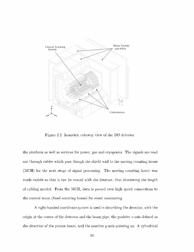
2.2 Overview of the D� Detector

The D� detector was designed to measure the decay products of interest in

p�p collisions: electrons, photons, muons, parton jets, and missing transverse energy

(E/T ) which signals the presence of non-interacting particles such as neutrinos. The

detector is composed of three subsystems: the tracking detectors, the calorimeter

and the muon spectrometer (Figure 2.2). The design of the detector emphasized

�nely segmented, hermetic calorimetry for the sole measurement of particle ener-

gies. Because of this the tracking volume is compact and has no magnetic �eld for

momentum measurement. The detector is described in detail in Reference [40] and

this description is well complimented by Reference [41].

The detector is mounted on a movable platform for movement in and out

of the collision hall. The �rst stage of detector readout electronics are mounted on

29

Calorimeters

Central Tracking System

Muon Toroids and PDTs

xz

y

Figure 2.2: Isometric cutaway view of the D� detector.

the platform as well as services for power, gas and cryogenics. The signals are read

out through cables which pass though the shield wall to the moving counting house

(MCH) for the next stage of signal processing. The moving counting house was

made mobile so that it can be moved with the detector, thus shortening the length

of cabling needed. From the MCH, data is passed over high speed connections to

the control room (�xed counting house) for event monitoring.

A right-handed coordinate system is used in describing the detector, with the

origin at the center of the detector and the beam pipe, the positive z-axis de�ned as

the direction of the proton beam, and the positive y-axis pointing up. A cylindrical

30

coordinate system is also used, with � measured with respect to the positive x-axis,

and � measured from the positive z-axis.

In describing the kinematics of detected particles several approximations are

taken for convenience. For a particle not at rest in the lab frame with energy E and

momentum p, the rapidity y is de�ned as

y =1

2lnE + pzE � pz

: (2.1)

In the limit p >> m, it is possible to approximate the rapidity as follows

y � � ln tan�

2� �: (2.2)

where � is called the pseudorapidity. The polar angle is often expressed in terms of

\detector pseudorapidity", denoted �det, which is referenced to z = 0. The interac-

tion point does not always coincide with the center of the detector, making � and

�det slightly di�erent.

In p�p collisions, the momenta of the colliding partons along the beam cannot

be reconstructed since many of the remnants of the collision are carried away down

the beam pipe. It is convenient then to use the transverse momentum, which is

the projection of the momentum vector in a plane perpendicular to the beam axis,

pT = p sin � , instead of the momentum. If energy deposition in the calorimeter is

treated as a vector, it is convenient to de�ne the transverse energy, ET = E sin �.

The direction of ET can be taken as the direction of pT . Also, only the transverse

component of missing energy is measured.

31

In the following sections the detector subsystems are discussed in more detail,

with an emphasis placed on the subsystems used in this analysis.

2.3 The Central Detector

The Central Detector (CD), shown in Figure 2.3, is composed of four subsys-

tems. The Vertex Drift Chamber (VTX), the Transition Radiation Detector (TRD)

and the Central Drift Chamber (CDC) are cylindrical devices which are arranged

concentrically around the beam pipe and cover the region of large angles. The fourth

subsystem consists of two Forward Drift Chambers (FDC) which are oriented per-

pendicularly to the beam pipe. The CD occupies a volume bounded by 3.7 cm < r <

75 cm and jzj < 135 cm.

In the absence of a central magnetic �eld, the momenta of particles are not

measured by the tracking chambers. Instead the tracking chambers were designed for

good two-track resolution, high e�ciency and good ionization energy measurement.

The TRD was added for additional rejection of isolated pions as a background for

electrons.

The tracking detectors were designed to match the 3.5 �s interval between

beam crossings. Flash analog-to-digital converters were used to digitize the signal

in 10 ns intervals to obtain good two-track resolving power.

Three of the four tracking detectors are wire drift chambers: the VTX, the

32

ΘΦ Central DriftChamber

Vertex DriftChamber

TransitionRadiationDetector

Forward DriftChamber

Figure 2.3: Side view of the D� central tracking detectors.

CDC and the FDC. The reader is referred to [42] for a detailed discussion of the

principles of drift chambers. An overview of the principles of wire drift chambers is

presented below.

As a charged particle passes through a gas it interacts electromagnetically

with nearby atomic electrons. This process produces ion-electron pairs along the

trajectory of the particle. In the presence of an electric �eld the electrons will

drift toward the positive electrode wire, called a sense wire. The ions drift in the

opposite direction but their drift velocity is considerably slower than that of electrons

making it safe to ignore their motion. In a multiwire drift chamber several such

33

drift wires are strung in parallel. The ionized electrons drift to the closest wire to

the point of their creation. A small diameter sense wire produces a very strong

electric �eld near it. This strong �eld accelerates drift electrons to energies high

enough to produce further ionization. In this manner, the number of electrons

increases exponentially producing an avalanche of electrons, thus giving rise to a

large measurable electrical current whose size is proportional to the original number

of ion-electron pairs created. The ratio of the number of electrons collected and the

number of electrons produces initially is referred to as the gas gain, and it typically

of the order of 104 to 106.

The drift velocity of the electrons is independent of the particle that produced

the ionization, but it is dependent on the strength of the electric �eld and the gas

composition, temperature and pressure. The drift time, the di�erence between the

known collision time and the arrival time of the pulse in the sense wire, is combined

with the drift velocity in order to infer the drift distance of the electrons. It is

necessary to ensure a constant electric �eld over as large a volume as possible in

order to obtain a linear relationship between distance and time. Additional �eld

shaping cathodes are inserted in order to make the �eld more uniform. From the

inferred drift distances, the trajectories of charged particles are reconstructed.

The reader is encouraged to read [42, 43, 44] for further discussion of drift

chambers and their application in high energy physics.

34

2.3.1 Vertex Drift Chamber

The Vertex Drift Chamber (VTX) [45, 46, 47] is the innermost of D�'s

tracking chambers. It was designed to provide precise determination of the location

of interaction vertices. Occupying the region 3.7 cm < r < 16.2 cm, it is composed

of three concentric and cylindrical layers with the inner layer measuring 97 cm in

length and each successive layer being about 10 cm longer. A cross section of one

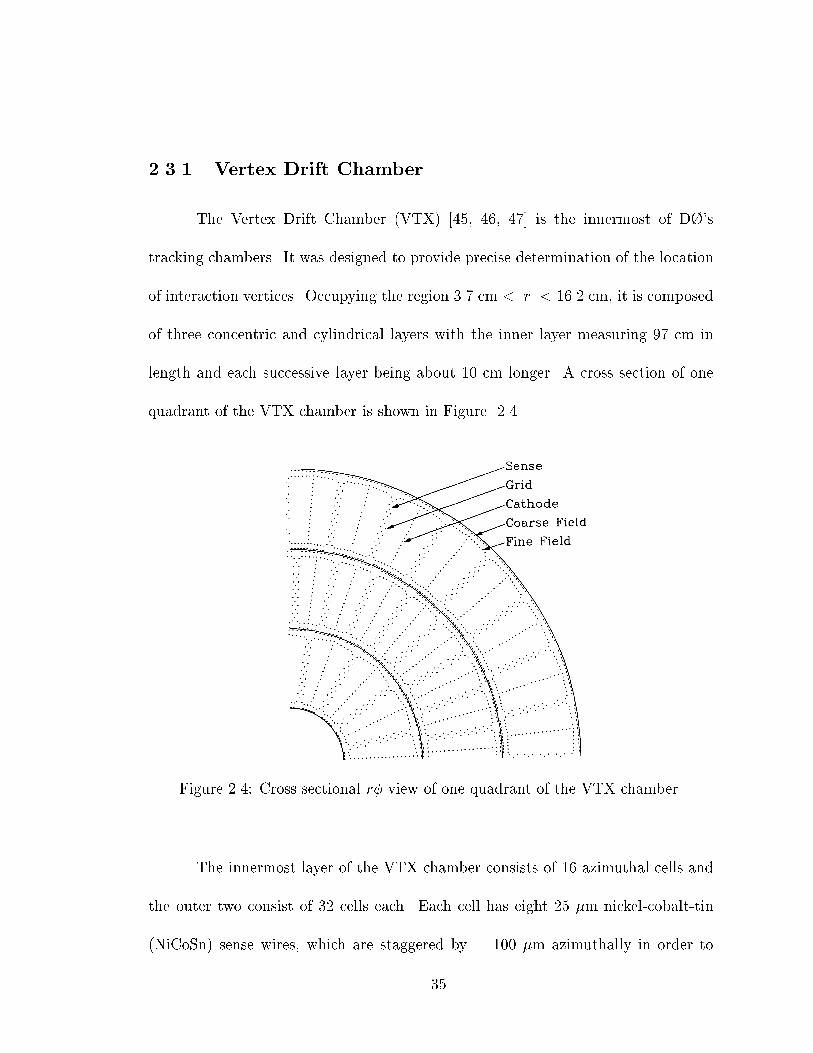
quadrant of the VTX chamber is shown in Figure 2.4.

Figure 2.4: Cross sectional r� view of one quadrant of the VTX chamber.

The innermost layer of the VTX chamber consists of 16 azimuthal cells and

the outer two consist of 32 cells each. Each cell has eight 25 �m nickel-cobalt-tin

(NiCoSn) sense wires, which are staggered by � 100 �m azimuthally in order to

35

resolve left-right ambiguity. Cells are o�set azimuthally in each successive layer to

further enhance pattern recognition. The r� coordinate of a hit is determined from

drift time and wire position with a position resolution of approximately 60 �m.

The z-coordinate is determined from charge division along the wire. However, the

observed z-position resolution was poor in a high luminosity environment and the

VTX was not used for determination of the primary vertex z position.

2.3.2 Transition Radiation Detector

The Transition Radiation Detector (TRD) [48, 49] occupies the space just

beyond the radius of the VTX. The TRD is primarily used to distinguish electrons

from charged pions. The TRD measures the emission of transition X-rays by highly

relativistic charged particles ( > 103) when they cross the boundary separating

media with di�erent dielectric constants. The TRD was not used in this analysis

because of the need to retain high e�ciency.

2.3.3 Central Drift Chamber

The outermost tracking detector, the Central Drift Chamber (CDC) [46, 50,

51, 52] consists of four cylindrical, concentric layers. The CDC provides trajectory

and ionization information on isolated charged particles out to a detector pseudo-

rapidity of j�detj < 1:2. The CDC occupies the radial region between 49.5 cm and

74.5 cm and is 184 cm in length.

36

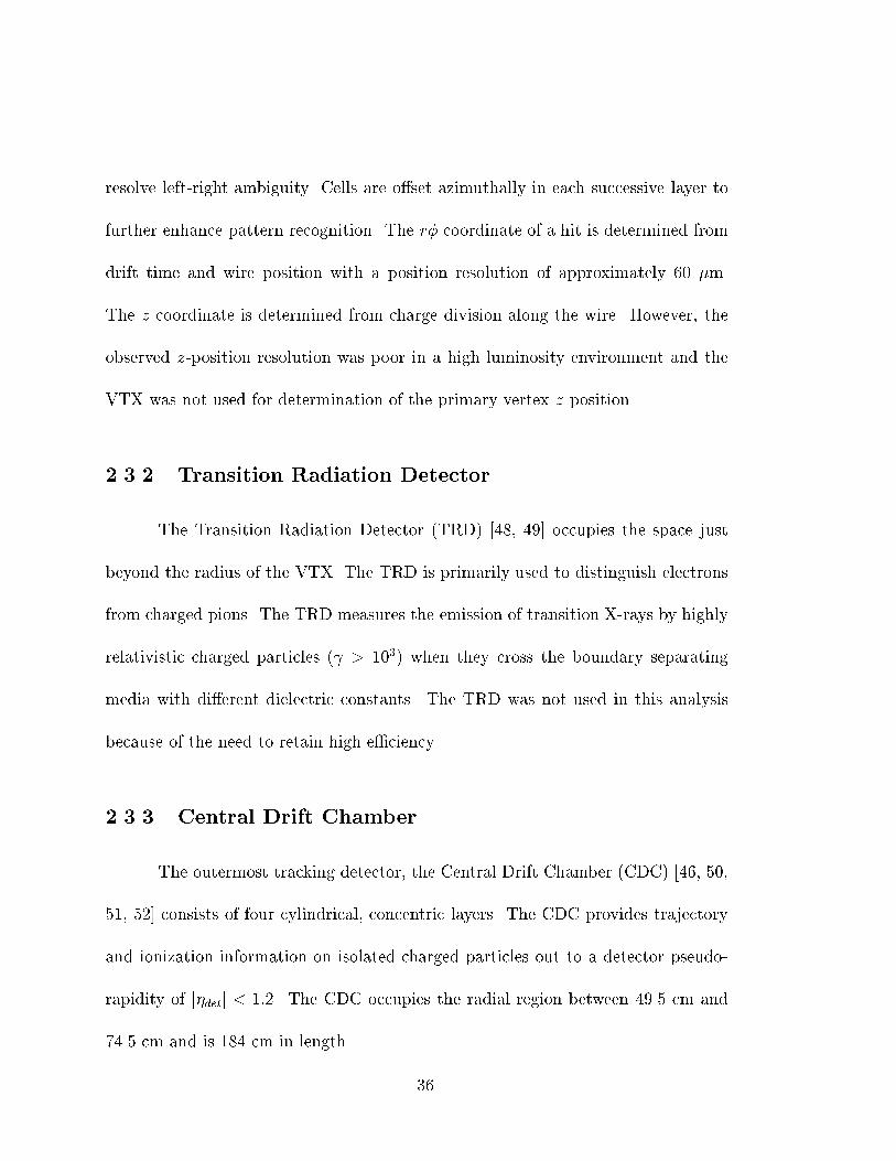
Each CDC layer is divided into 32 modular, azimuthal cells. A cross section

of three such cells is shown in Figure 2.5. Each cell contains seven 30 �m gold-plated

tungsten sense wires and two delay lines. The sense wires are staggered by � 200 �m

azimuthally to reduce left-right ambiguity and alternate cells are o�set azimuthally

by half a cell to enhance pattern recognition. The r� coordinate of a hit is obtained

from the drift time information and from the wire hit. The z position is inferred

via the use of delay lines. Whenever an avalanche occurs near a delay line a pulse

is induced in the delay line. The di�erence in the arrival times at both ends of the

delay line gives an estimate of where along the delay line the hit occurred. The r�

and z resolutions are approximately 180 �m and 2.9 mm respectively.

Figure 2.5: End view of three CDC modules. Sense wires are indicated by smalldots, guard (�eld shape) wires by large dots, and delay lines by open circles.

37

2.3.4 Forward Drift Chambers

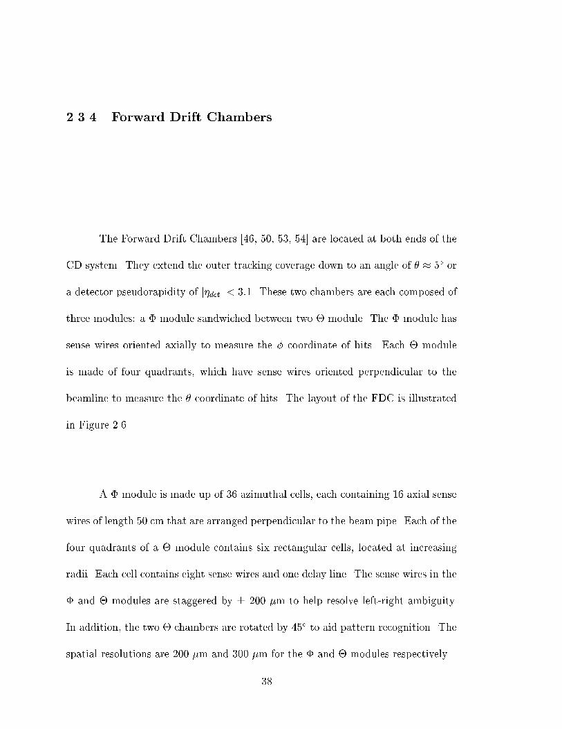
The Forward Drift Chambers [46, 50, 53, 54] are located at both ends of the

CD system. They extend the outer tracking coverage down to an angle of � � 5� or

a detector pseudorapidity of j�detj < 3:1. These two chambers are each composed of

three modules: a � module sandwiched between two � module. The � module has

sense wires oriented axially to measure the � coordinate of hits. Each � module

is made of four quadrants, which have sense wires oriented perpendicular to the

beamline to measure the � coordinate of hits. The layout of the FDC is illustrated

in Figure 2.6.

A � module is made up of 36 azimuthal cells, each containing 16 axial sense

wires of length 50 cm that are arranged perpendicular to the beam pipe. Each of the

four quadrants of a � module contains six rectangular cells, located at increasing

radii. Each cell contains eight sense wires and one delay line. The sense wires in the

� and � modules are staggered by � 200 �m to help resolve left-right ambiguity.

In addition, the two � chambers are rotated by 45� to aid pattern recognition. The

spatial resolutions are 200 �m and 300 �m for the � and � modules respectively.

38

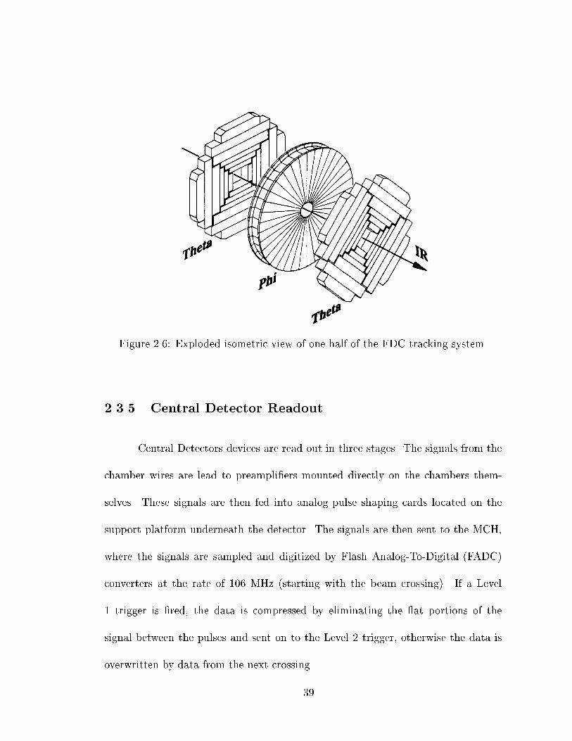
Figure 2.6: Exploded isometric view of one half of the FDC tracking system.

2.3.5 Central Detector Readout

Central Detectors devices are read out in three stages. The signals from the

chamber wires are lead to preampli�ers mounted directly on the chambers them-

selves. These signals are then fed into analog pulse shaping cards located on the

support platform underneath the detector. The signals are then sent to the MCH,

where the signals are sampled and digitized by Flash Analog-To-Digital (FADC)

converters at the rate of 106 MHz (starting with the beam crossing). If a Level

1 trigger is �red, the data is compressed by eliminating the at portions of the

signal between the pulses and sent on to the Level 2 trigger, otherwise the data is

overwritten by data from the next crossing.

39

2.4 Calorimetry

The Calorimeter system at D� is the most crucial part of the D� detector

since it provides the only means to measure the energy of electrons, photons, and

jets. Furthermore, it plays a vital role in the identi�cation of neutrinos through the

transverse imbalance of energy.

A calorimeter is a block of material which is placed in the path of a particle

and is of su�cient thickness to cause it to interact and deposit all of its energy in

the medium. Some percentage of the energy deposited is detectable in the form of

scintillation light or ionization charge which is proportional to the incident energy

of the particle.

At energies above 1 GeV, photons and electrons dissipate their energy at an

energy independent rate via electron-positron pair production and Bremsstrahlung

respectively. An incident electron or photon will produce a shower of secondary

particles by these loss mechanisms. For example an electron will produce a photon,

which will in turn produce a electron-positron pair, which in turn will produce

photons, etc. This process will continue until all secondary particles drop below

the energy at which ionization of the medium becomes the primary energy loss

mechanism.

The energy loss �E by radiation in a length �x can be written as

(�E)raditation = �E(�x=X�)

40

where X� is the \radiation length" of a material. The radiation length is approxi-

mated by

X�[g=cm2] � 180A=Z2:

The energy loss by ionization in a medium is characterized by the \critical

energy" � below which ionization losses dominate. The energy loss by an elec-

tron/positron of energy � in medium in radiation length X� is given by

(dE)collision = ��(dx=X�)

where �(MeV) � 500=Z.

The total track length of secondaries in an electromagnetic shower is given

by T = (E=�)X� with the peak multiplicity of the shower occurring at

� (ln (E=�) � 2) X�:

The transverse pro�le of a shower is characterized by the typical angle for

bremsstrahlung emission and multiple scattering in the medium. About 90% of the

total energy of a shower is contained within a cylinder of radius 2�M , where

�M = 21X�=� � 7A

Z[g cm�2]

is the \Moliere Radius", which is the average lateral de ection of electrons of energy

� after traveling one radiation length.

Two types of calorimeter can be used to measure the energy of particles. A

homogeneous calorimeter is composed of one material such as sodium iodide (NaI)

41

or lead glass. A sampling calorimeter uses a dense passive absorber interspersed

with an active medium which samples the energy of the shower at various points

in its development. A homogeneous calorimeter can achieve a better energy resolu-

tion than a sampling calorimeter, but a sampling calorimeter is usually much more

compact than a homogeneous calorimeter because of the dense absorber.

The energy resolution of a sampling calorimeter is limited by the statistical

uctuations of the amount of ionization in the sampling layers. The fractional error

in the energy is proportional to one over the square root of the number of ionizing

tracks or equivalently, E� 12 .

The energy measurement of hadronic showers is conceptually analogous to

electromagnetic showers. Hadrons interact by inelastic collisions with atomic nuclei

in the medium, producing secondary hadrons which repeat the process, creating a

shower of hadronic particles. The greater variety and complexity of the hadronic

processes propagating the shower make an analytic description di�cult. We can

however give some general features.

The scale for hadronic interactions is the nuclear interaction length

�A � 35A1=3[g=cm2]:

The average shower maximum occurs at � (0:2 lnE+0:7)�A where E is measured in

GeV. About 90% of the energy is contained within 2.5�A of the shower maximum.

In the transverse direction, 95% of the energy is contained within a cylinder of radius

42

R � 1�A.

Fluctuations in the constituent particles of hadronic showers are the principal

limitation to the energy resolution. The response of a calorimeter will di�er for

hadrons and electrons of the same energy. If the fraction of �0's and �0's produced

in the �rst interaction is large, most of the energy will be measured as these particles

quickly decay to two photons. If the interactions produce muons and neutrinos,

most of the energy will be carried away. Thus the calorimeter response to hadrons

is typically less than for electrons. This di�erence, the \e/h ratio", can be corrected

for on average, but a ratio di�erent from one will result in uctuations on a shower

by shower basis. An e/h ratio near unity can be achieved by decreasing the electron

response or boosting the hadronic response. The latter can be achieved by using

uranium-238, because secondary neutrons can cause �ssion in the uranium nuclei

which produces some visible energy.

For further discussions on calorimeters, the reader is referred to [43, 44], as

well as articles [55, 56].

2.4.1 Calorimeter Design

The D� Calorimeter is a sampling calorimeter. Liquid argon (LAr) was

chosen as the active medium because of its unit gain, simplicity of calibration,

exibility in the segmentation of readout cells and resistance to radiation damage.

The use of LAr requires a containment vessel (cryostat), where the argon is kept cold

43

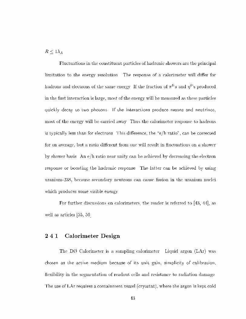
enough to remain in the liquid form. As shown in Figure 2.7, the Calorimeter was

split into three modules, one Central Cryostat (CC) covering the region j�j < 1:2,

two Endcap Cryostats (EC) extending the coverage to j�j � 4. This was done to

retail access to the tracking detectors. The design left an uninstrumented region

between the cryostats. The Inter-cryostat Detector (ICD) was built to cover this

region.

1m

CENTRALCALORIMETER

END CALORIMETER

Outer Hadronic(Coarse)

Middle Hadronic(Coarse & Fine)

Inner Hadronic(Coarse & Fine)

Electromagnetic

Coarse Hadronic

Fine Hadronic

Electromagnetic

Figure 2.7: Isometric view of D� calorimetry.

The D� Calorimeter is highly modular, and �nely segmented in the trans-

verse and longitudinal shower directions. Three distinct types of modules are used

44

in the CC and EC: an electromagnetic section (EM) with thin uranium-238 ab-

sorber plates, a �ne hadronic section (FH) with thicker uranium plates and a coarse

hadronic section (CH) with thick copper or stainless steel plates.

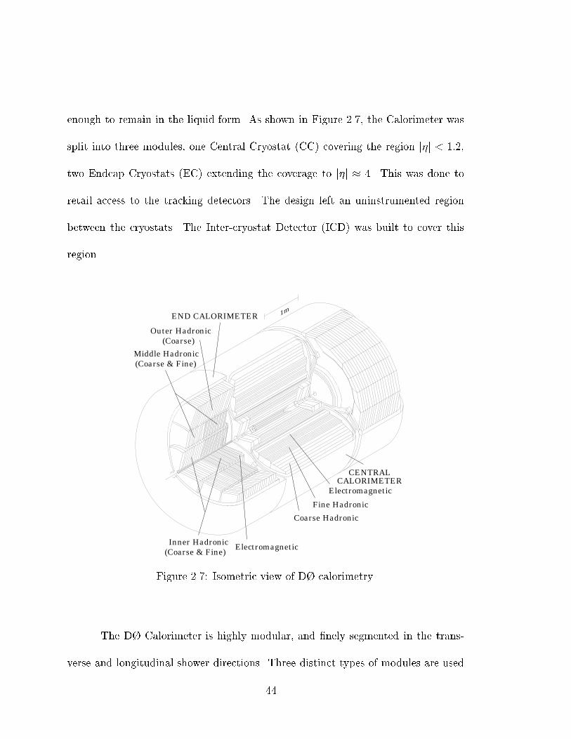
Each module consists of a row of alternating absorber plates and signal read-

out boards, as shown in Figure 2.8. An electric �eld is established by grounding the

absorber plate while applying a positive potential (typically 2.0-2.5 kV) to the re-

sistive surfaces of the signal boards. The 2.3 mm gap was chosen to be large enough

to observe a minimum ionizing particle in the LAr. The ionization electrons drift

across the gap in � 450 ns.

G10 InsulatorLiquid Argon

GapAbsorber Plate Pad Resistive Coat

Unit Cell

Figure 2.8: Schematic view of a D� calorimeter cell.

45

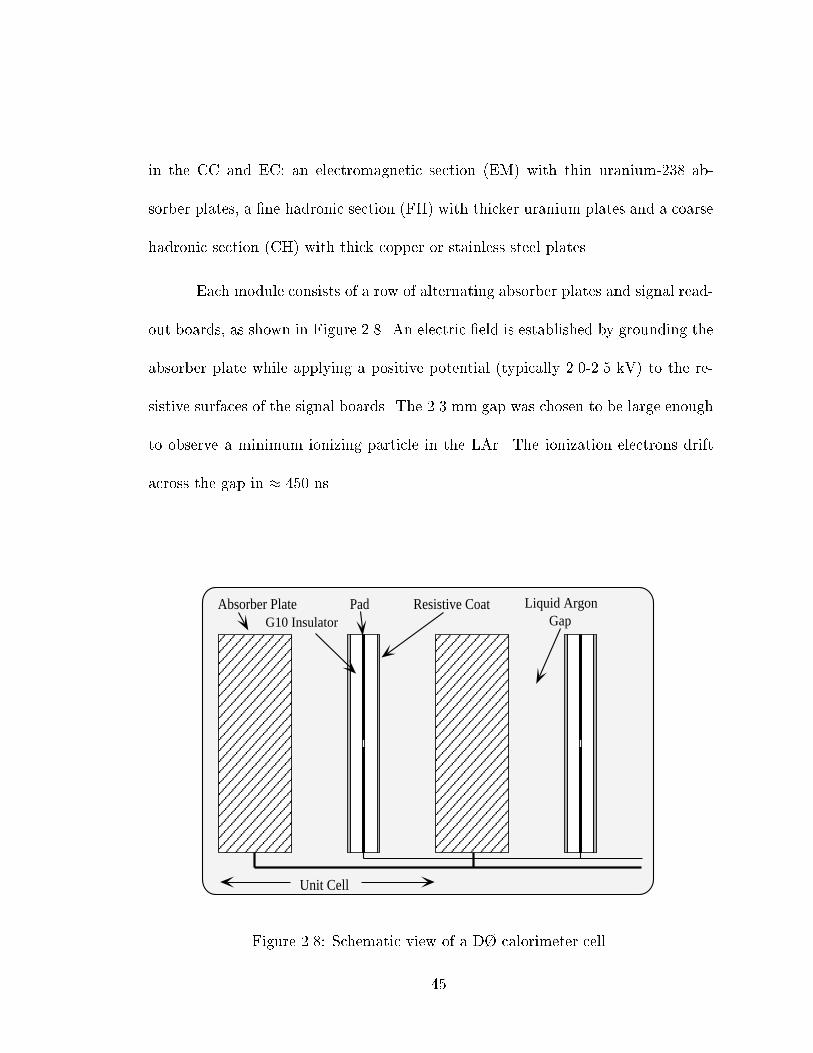
The pattern and sizes of the readout cells were determined from considera-

tions of shower sizes. The transverse dimensions of the readout cell were chosen to

be similar to the transverse sizes of showers: � 1{2 cm for EM showers and � 10 cm

for hadronic showers. Longitudinal segmentation within the EM, FH and CH layers

helps in the distinction and separation of electrons from hadrons. The design was

chosen to be \pseudo-projective": the centers of the cells lie on lines which project

back to the center of the detector, but the cell boundaries are aligned perpendicular

to the absorber plates. This is clearly illustrated in Figure 2.9.

Figure 2.9: Side view of one quadrant of the calorimeter and central detector. Thelines of constant pseudorapidity intervals are with respect to z = 0.

46

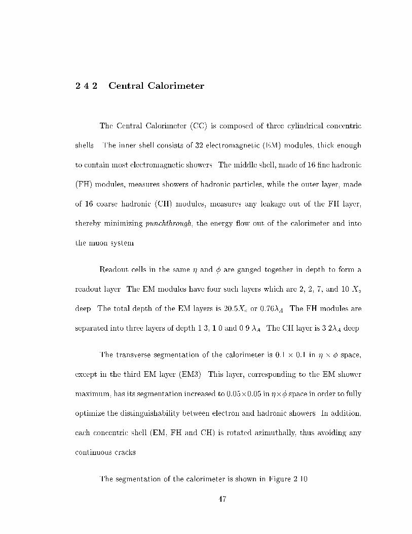
2.4.2 Central Calorimeter

The Central Calorimeter (CC) is composed of three cylindrical concentric

shells . The inner shell consists of 32 electromagnetic (EM) modules, thick enough

to contain most electromagnetic showers. The middle shell, made of 16 �ne hadronic

(FH) modules, measures showers of hadronic particles, while the outer layer, made

of 16 coarse hadronic (CH) modules, measures any leakage out of the FH layer,

thereby minimizing punchthrough, the energy ow out of the calorimeter and into

the muon system.

Readout cells in the same � and � are ganged together in depth to form a

readout layer. The EM modules have four such layers which are 2, 2, 7, and 10 X�

deep. The total depth of the EM layers is 20:5X� or 0:76�A. The FH modules are

separated into three layers of depth 1.3, 1.0 and 0.9 �A. The CH layer is 3.2�A deep.

The transverse segmentation of the calorimeter is 0:1 � 0:1 in � � � space,

except in the third EM layer (EM3). This layer, corresponding to the EM shower

maximum, has its segmentation increased to 0:05�0:05 in ��� space in order to fully

optimize the distinguishability between electron and hadronic showers. In addition,

each concentric shell (EM, FH and CH) is rotated azimuthally, thus avoiding any

continuous cracks.

The segmentation of the calorimeter is shown in Figure 2.10.

47

Figure 2.10: Longitudinal tower segmentation of the D� calorimeter as a functionof pseudorapidity.

2.4.3 Endcap Calorimeters

The two Endcap Calorimeters (EC) provide coverage on either side of the

CC. Each endcap cryostat is divided into four sections: the electromagnetic (EM)

module in front of the inner �ne hadronic (IH), the middle hadronic (MH), and

outer hadronic (OH) modules.

The EM module is a disk composed of four layers with an inner radius of 5.7

cm and an outer radius varying between 84 and 104 cm. The four layers are 0.3,

2.6, 7.9 and 9.3 X� in depth. The transverse segmentation is 0:1� 0:1 in � � � for

48

j�detj < 3:2, after which it doubles. As in the CC, the segmentation in the third EM

layer is �ner. The segmentation in this layer is 0:05� 0:05 for j�detj < 2:7, 0:1� 0:1

for 2:7 < j�detj < 3:2 and 0:2� 0:2 for j�detj > 3:2.

The inner hadronic modules are cylindrical with inner radius 3.93 cm and

outer radius 86.4 cm. The �ne hadronic portion has four layers, each 1.1�A thick.

Alternate layers are rotated by 90� to avoid cracks. The coarse hadronic section has

one layer with stainless steel plates of depth 4.1�A.

The middle hadronic modules surround the inner hadronic modules. The

�ne hadronic portion consists of four layers with uranium plates of depth 0.9�A

each and the coarse hadronic section consists of one layer with stainless steel plates

4.1�A deep.

The outer hadronic modules surround the middle hadronic layer. There are

three coarse layers with stainless steel plates inclined at 60� to the beamline. The

depth of each layer is 4.1�A deep.

The the transverse segmentation of the inner hadronic layers is 0:1� 0:1 for

j�detj < 3:2 and 0:2 � 0:2 otherwise. Beyond the EM coverage (j�detj > 3:8) the

segmentation is 0:4 � 0:2. The segmentation for the middle and outer hadronic

layers is 0:1� 0:1.

The reader is referred to Figures 2.9 and 2.10 for a layout of the calorimeter

modules.

49

2.4.4 Intercryostat Detectors and Massless Gaps

The region of crossover between the CC and EC (0:8 � j�detj � 1:4) contains

a large amount of uninstrumented material. To correct for energy deposited in this

uninstrumented region, two scintillation arrays called intercryosts detectors (ICD)

were mounted on the front surface of each EC. Each consists of 384 tiles of size

�� = �� = 0:2. In addition, rings of readout boards, called massless gaps, were

mounted on the endplates of the CC FH modules and the EC MH and OH modules

to record any ionization caused by the cryostat walls acting as absorbers.

2.4.5 Calorimeter Readout

Signals from the calorimeter modules are readout in several stages. They

are �rst brought to feedthrough boards in the cryostat walls to charge-sensitive

preampli�ers and then via twisted pair cable to baseline subtracter (BLS) shaping

and sampling circuits. The signals are integrated (430 ns) and di�erentiated (33 �s).

The signals are sampled just before and 2.2 �s after a beam-crossing. The di�erence

is proportional to the collected charge. The signals are then sent to the moving

counting house where ADC's digitize each signal into 384 channels. Channels which

fall below a threshold can be suppressed from further readout to reduce bandwidth.

A portion of the signal is sampled at the BLS input and added into �� = �� = 0:2

trigger towers for use in event selection.

50

2.4.6 Calorimeter Performance

The energy resolution of electrons and pions with energies between 10 and 150

GeV were measured using Endcap Calorimeter electromagnetic and �ne hadronic

modules in test beam conditions. The measured resolutions can be approximated

by:

�(E)

E� 16%p

Efor electrons

�(E)

E� 41%p

Efor pions:

These approximations show the expected E� 12 response due to the statistical

uctuations in the showers, but do not take into account noise and calibration

uncertainties which must be measured in situ. The resolution for single pions is a

lower limit on the resolution for jets which are composed of many hadrons.

The e/h ratio was measured to fall from 1.11 at 10 GeV to 1.04 at 150 GeV

after accounting for out-of-time event pile-up, early showering and energy deposition

outside the � � � region used to sum energies.

The calorimeter position resolution is important in matching tracks with

calorimeter clusters for the rejection of backgrounds to electrons. The position

resolution was found using the energy weighted position of the shower as measured

by EM layer 3 for 100 GeV electrons. The resolution varied between 0.8 and 1.2 mm

depending on entry angle and varied with energy as E12 .

51

2.5 Muon Tracking

Muons do not interact via the strong force and are too massive to lose sub-

stantial energy via Bremsstrahlung. With a long lifetime (� = 2:2�s), they can

traverse the entire thickness of the detector without decaying. In traversing the

calorimeter they leave a minimum ionizing particle trace.

The muon tracking system uses proportional drift tubes (PDT) and �ve mag-

netized iron toroidal magnets to measure the momenta of passing muons [57]. The

�rst layer of PDT's is placed inside the magnets and two layers are placed outside

the magnets to measure the bend in a muon's trajectory and thus its momentum.

The muon system is subdivided into two sections, the wide angle muon system

(WAMUS) and the small angle muon system (SAMUS), which are described below.

2.5.1 WAMUS

The WAMUS contains rectangular PDT's which have one sense wire per

drift cell. The WAMUS region extends to j�detj � 1:7. The three layers, A, B,

and C (shown in Figure 2.11), are composed of 4, 3, and 3 planes of drift tubes

respectively. The readout electronics measure the arrival times of pulses as well as

the di�erence of arrival times at the end of each cell. This time di�erence is used

to give a rough determination of the position along the wire where a hit occurred.

A more precise measurement of the hit position can be made using vernier cathode

52

pads in each tube. By measuring the division of charge between the inner and outer

pad, a position measurement with resolution of about 3 mm can be made along the

direction of the wire. The position measurement perpendicular to the sense wire

has an accuracy of about 0.53 mm.

Figure 2.11: Side view of the D� muon system.

The momentum of the muon is determined by reconstructing the trajectory

from hits in the three layers. The momentum resolution is dependent on the accuracy

of the trajectory measurement and multiple scattering in the magnets, which smears

the direction of the muon as it exits the magnets.

53

2.5.2 SAMUS

The SAMUS covers a pseudorapidity range of 1:7 � j�detj � 3:6. Due to the

higher ux of particles in the forward region the SAMUS uses smaller drift tubes.

The system consists of three planes of drift tubes. Each plane is composed of two

subplanes o�set by half a tube diameter. The drift tubes are made of stainless steel

tubes with a 3 cm diameter, each with a single sense wire.

2.6 Trigger and Data Acquisition

During the 92-96 data taking run, the Tevatron was operated with a 3.5 �s

interval between bunch crossings. At the luminosities obtained, this resulted in one

or more interactions per crossing. It would be impossible to record every event at

this rate (� 286 Hz). The solution is to record only events of interest by \triggering"

on event characteristics of interest.

A schematic overview of the D� trigger system is shown in Figure 2.12. It

consists of three di�erent levels, each with increasingly sophisticated event charac-

terization. The Level 0 trigger uses a set of scintillation counters to indicate the

presence of an inelastic collision. It reduces the rate to about 150{200 kHz. The

Level 1 trigger is a collection of hardware triggers which is software programmable.

Most trigger decisions are made within the 3.5 �s interval between beam crossings.

However, some triggers, called Level 1.5 , may require additional time. The event

54

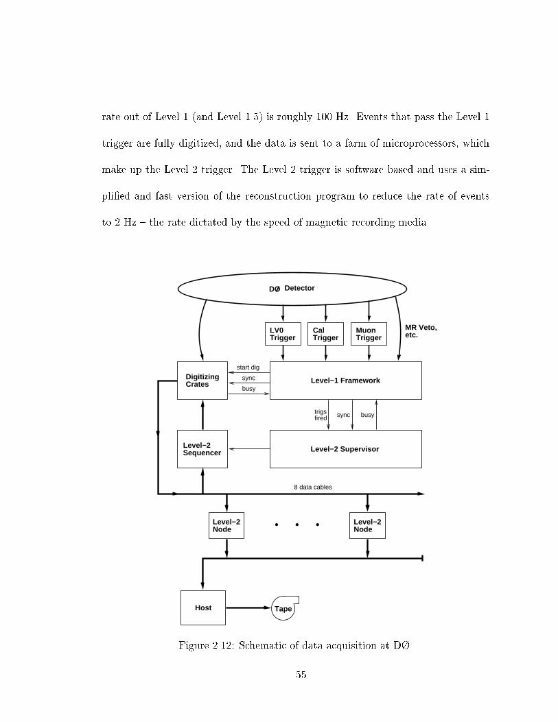
rate out of Level 1 (and Level 1.5) is roughly 100 Hz. Events that pass the Level 1

trigger are fully digitized, and the data is sent to a farm of microprocessors, which

make up the Level 2 trigger. The Level 2 trigger is software based and uses a sim-

pli�ed and fast version of the reconstruction program to reduce the rate of events

to 2 Hz { the rate dictated by the speed of magnetic recording media.

Level−2Node

Level−2Node

DO Detector

MR Veto,etc.

LV0Trigger

CalTrigger

MuonTrigger

8 data cables

Level−2 SupervisorLevel−2Sequencer

busysynctrigsfired

Level−1 FrameworkDigitizingCrates

sync

busy

start dig

Host Tape

Figure 2.12: Schematic of data acquisition at D�.

55

2.6.1 Level 0

The Level 0 trigger registers the presence of inelastic collisions and serves as

the luminosity monitor for the experiment. It consists of two hodoscopes of scintilla-

tion counters mounted on the front surfaces of the endcap calorimeters. Coincident

signals in both hodoscopes signals the presence of an inelastic collision. The Level 0

trigger also provides information of the z-coordinate of the interaction from timing

information. The luminosity is obtained from measuring the rate of inelastic colli-

sions with jzvtxj < 100 cm. This number is corrected for the acceptance of the Level

0 system modeled in Monte Carlo studies and then multiplied by the world average

for the total inelastic cross section [58]. The total error on the luminosity using this

method is 5.4%.

2.6.2 Beam Vetoes

As mentioned earlier, the Main Ring beam pipe passes through the upper

hadronic section of the Calorimeter. While collisions are occurring in the Tevatron,

the Main Ring is still in operation for �p production. During injection of protons into

the Main Ring and the transition to 150 GeV, losses are seen in the D� detector.

Losses are also seen during the passage of the proton beam during a Tevatron beam

crossing. This causes spurious hits in the coarse hadronic calorimeter (a�ecting the

E/T measurement) and in the muon system.

56

To account for these conditions, two trigger terms for the Level 1 framework

were developed to veto events occurring during Main Ring losses [59]. Speci�-

cally, events are rejected which occur within a 400 ms window after Main Ring

proton injection (MRBS LOSS) and within a 1.6 �s gate which occurs every 21�s

and is consistent with the passage of Main Ring protons through the D� detec-

tor (MICROBLANK). The beam veto which imposes both conditions is known as

\GOOD BEAM" since good beam conditions are required. The total dead time

incurred by the GOOD BEAM veto is about 25%.

2.6.3 Level 1

The Level 1 trigger [60] was designed to minimize the decision time as much

as possible so that no dead time was incurred for trigger decisions. The Level

1 framework gathers digital information from each Level 1 trigger device as well

as various vetoes. The trigger decision is made by a two-dimensional AND-OR

network. The network consists of 256 inputs and has 32 outputs which correspond

to the Level 1 triggers. These triggers are programmable, allowing the thresholds

and the pattern of input terms which �re the trigger to be modi�ed. Additionally,

a \prescale" can be speci�ed for triggers with high rates.

The Level 1 calorimeter trigger uses separate EM and �ne hadronic trigger

towers (both with ����� = 0:2�0:2 wide) as inputs to the AND-OR network. The

energy in the trigger towers is weighted by the trigger tower polar angle with respect

57

to z = 0 to give the transverse energy. The transverse energy is then corrected using

a z-vertex determined from the initial timing information from Level-0, if available.

The transverse energy of each tower is split into x- and y- components and the

components are summed over the entire calorimeter to determine E/T . The energies

of each tower as well as the total tower energy (EM+FH) and global sums are used

as inputs into the AND-OR network, where they are compared to the programmed

thresholds.

For this study, the trigger used required two EM towers with ET > 7 GeV

(the so-called EM 2 MED trigger). No events under this trigger were discarded for

the purposes of bandwidth management, i.e. this trigger was not prescaled during

data collection.

2.6.4 Level 1.5

The Level 1.5 trigger uses digital signal processors to re�ne and con�rm the

Level 1 trigger decision [61]. The Level 1.5 calorimeter trigger improves energy

resolution by examining the energy in towers neighboring the Level 1 EM towers.

Additionally, energy sums are computed from adjacent hadronic towers, and the

ratio EEM=E is used for further background rejection. For this analysis, events

passing the EM 2 MED Level 1 trigger were required to have at least one Level 1.5

electron candidate with ET > 12 GeV and EEM=E > 0:85.

58

2.6.5 Level 2

The Level 2 system functions as the next layer of event �ltering and the

data acquisition system with the goal of reducing the rate of events recorded to

tape to 2 Hz. The Level 2 system consists of a cluster of 48 dedicated CPU nodes

connected to 8 high speed data cables for reading out the event information from the

digitization crates. If an event passes a Level 1(1.5) trigger, the Level 2 supervisor

node �nds a free Level 2 node and tells it to start reading out the event information

from over the eight data cables, each corresponding to one of the eight detector

sections: VTX, TRD, CDC, FDC, the north and south halves of the calorimeter,

muon chambers, and Level 0 and Level 1 triggers. If an event passes a Level 2 �lter

it is passed to the host computer for recording on magnetic media.

The Level 2 nodes run an event-�ltering program which is built around a

series of �lter tools. Among the tools are those for jets, calorimeter EM clusters,

track association with calorimeter clusters,PET and E/T . Speci�c combinations

and orders of these tools are combined into \scripts". Each script is associated with

one of the 32 Level 1 triggers. The script can generate several Level 2 �lters for a

given Level 1 trigger based on di�erent ET thresholds or other features of the event

like energy isolation or E/T . There are 128 Level 2 �lters available.

All events in this analysis are required to satisfy the EM2 EIS2 HI Level 2

software �lter. This �lter required two Level 2 electron candidates with ET >

59

20 GeV which satis�ed electron shower shape and isolation cuts.

2.7 Online Cluster

The D� online cluster [41] is composed of three VAX minicomputers. They

are dedicated to recording events on disk and spooling them to 8mm tape and

to hardware monitoring. The cluster also serves as the human interface to the

detector systems. In this role it is responsible for control of data taking, downloading

programmable parameters, and displaying of data from the detector which includes

calibrations, monitoring information and alarms.

2.8 O�ine Data Processing

The data is stored on high density 8mm magnetic tapes. The events are

reconstructed by the full event reconstruction program (described in the next chap-

ter) by a farm of Silicon Graphics and IBM computers at the Fermilab Central

Computing Facility. Two types of �les are produced by the reconstruction program.

STA �les contain the raw data plus the results of the reconstruction and contain

approximately 600 kilobytes per event. DST �les contain only the results of the

reconstruction such as calorimeter clusters and reconstructed tracks as well as pa-

rameters for electrons, jets, E/T etc. The DST event size is typically 30 kilobytes per

event. The size of the 93-95 data set brought about the need for an even smaller

60

event format called �DST which contained only the most essential information for

analysis. The STA �les are kept on tape, and the DST �les are kept on disk on a �le

server cluster. From here the data are �ltered into separate streams, depending on

high level event characteristics, and are stored in �DST format for further analysis.

61

Chapter 3

Event Reconstruction and Particle

Identi�cation

The information recorded by the D� detector is in the form of digital signals:

pulse heights, widths and times. These signals are converted into numbers useful to

an analysis by a standard reconstruction program called D�RECO, which converts

the signals into tracks and calorimeter clusters which are then interpreted as jets,

electrons, photons, muons and neutrinos (E/T ). A brief description of the steps taken

in event reconstruction are described below. Following that is a description of the

variables used for identifying electrons.

62

3.1 Track Reconstruction

Tracks in the Central Detector are reconstructed in four stages: hit �nding,

segment �nding, segment matching, and global track �tting. The arrival time and

drift time of a pulse are used to �x the location of a hit, and the integral of a pulse

is used to determine charge deposition. All pulses are converted to hits, and track

�nding proceeds. Within each layer hits are grouped together into a segment using

roads in the r{� plane. If enough hits are found within the road which �t to a line

with small enough variation, a segment is formed. If three of four segments �t a

straight line, a track is formed.

The direction of a track is speci�ed by a reference point, called the track

centroid, and two angles. The track centroid is corrected for biases in z-coordinate

using cosmic muons and collider muons [64, 65]. Tracks in the forward region are only

reconstructed in a wide road de�ned by a calorimeter cluster and the event vertex.

In the central regions, all hits are considered for track reconstruction. Further details

regarding central detector hit �nding and tracking can be found in References [51,

52, 53, 54].

3.2 Vertex Finding

The next step in the event reconstruction process is to determine the number

and z-position of event vertices. This is done by creating a histogram of CDC

63

track z-intercepts (see Figure 3.1). The primary vertex is identi�ed as the peak

with the largest number of associated tracks. All high-ET objects are assumed to

arise from the primary vertex. Any other peaks are identi�ed as secondary vertices

resulting from minimum bias interactions. The z-resolution attained is 1{2 cm, with

multiple vertices resolvable down to 7 cm. In a high-luminosity environment where

multiple interactions occur, the high-ET interaction of interest may have a lower

number of charged tracks than the other minimum bias interactions in the event.

For luminosities typical during the 93-96 data taking runs (� 7 �1030 cm�2s�1), 70%

of all events contained more than one interaction. A method of vertex determination

which relies on the information from high-ET objects is preferred. A discussion of

one such method which uses electrons will be discussed in Section 3.10.2.

The (x,y) coordinate of the vertex was not recorded. Instead the (x,y) co-

ordinate of the beam spot was recorded for each store. A slight o�set in the beam

had no noticeable e�ect on high-ET object events.

3.3 Calorimeter Hit Finding

Only cells in the calorimeter with energy above the noise threshold are exam-

ined. Pulse heights are converted into energy deposited using calibration constants

determined in test beam studies.

64

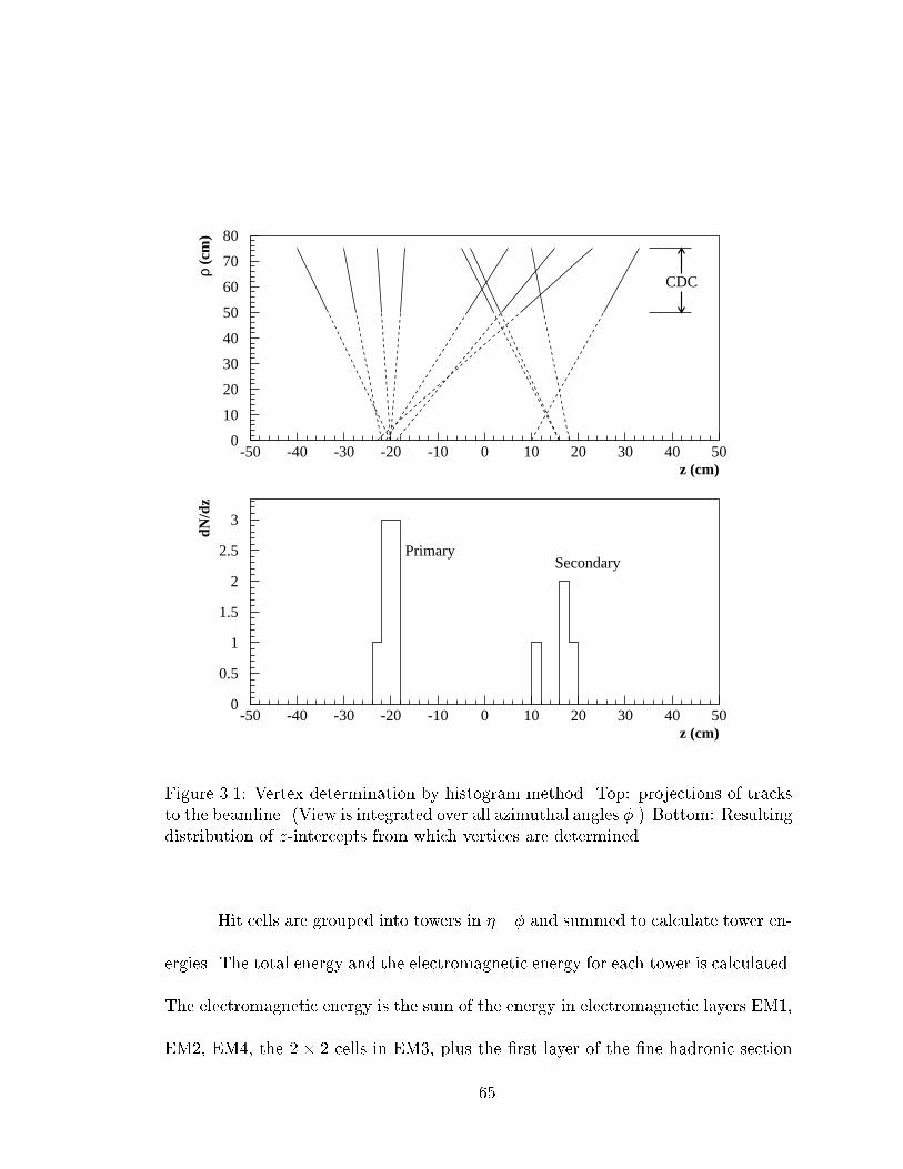
z (cm)

ρ (c

m)

CDC

z (cm)

dN/d

z

PrimarySecondary

0

10

20

30

40

50

60

70

80

-50 -40 -30 -20 -10 0 10 20 30 40 50

0

0.5

1

1.5

2

2.5

3

-50 -40 -30 -20 -10 0 10 20 30 40 50

Figure 3.1: Vertex determination by histogram method. Top: projections of tracksto the beamline. (View is integrated over all azimuthal angles �.) Bottom: Resultingdistribution of z-intercepts from which vertices are determined.

Hit cells are grouped into towers in ��� and summed to calculate tower en-

ergies. The total energy and the electromagnetic energy for each tower is calculated.

The electromagnetic energy is the sum of the energy in electromagnetic layers EM1,

EM2, EM4, the 2� 2 cells in EM3, plus the �rst layer of the �ne hadronic section

65

FH1. These towers form the basis for jet and electron/photon clustering.

3.4 Missing Energy

The presence of a neutrino or any other minimally interacting particle is

inferred by an imbalance of energy in the event. Because the energy of the spectator

quarks, which escape down the beam pipe, is not recorded by the detector, only the

transverse component of this energy imbalance can be fully reconstructed.

To determine this transverse energy imbalance all calorimeter cell energies

are treated as vectors using the primary event vertex and the cell center to determine

vector direction and cell energy to determine vector magnitude. Then the transverse

components of vectors are summed. The missing transverse energy vector exactly

balances this vector sum. Three versions of missing energy are calculated. The �rst

version is calculated from calorimeter cells only. The second version corrects for

energy deposited in the ICD cells. The third version subtracts out the momentum

of any muons in the event.

3.5 Jet Reconstruction

Hadrons produce a shower of secondary hadrons, called a jet, in the calorime-

ter. The most common de�nition of a jet at D� uses a cone to de�ne which cells

will be summed to give the original hadron energy. For this analysis a cone size of

66

R =p��2 +��2 = 0:5 was used.

The cone algorithm begins by picking towers with the highest ET as cluster

seeds. The cells within � � � = 0:3 � 0:3 of the seed tower are summed to form

pre-clusters. All seed towers within the precluster are dropped from the seed tower

list. The next highest ET seed tower is used to de�ne a new precluster. This process

is continued until all towers are used. The energies of cells within the cone centered

on each precluster are summed using ET weighting to determine a shower centroid.

The jet is reclustered using the newly calculated centroid to de�ne the cone until

the direction of the shower centroid stabilizes. A cone must contain at least 8

GeV of energy to be identi�ed as a jet. If two jets overlap, they are merged if the

energy of the overlapping cells is more than 50% of the energy of the lower ET jet.

Otherwise the energy of the overlapping cells are assigned to the jet with the closer

shower centroid. This merging/splitting process is continued until all preclusters

are assigned to a jet. The kinematic properties of the jet are calculated by summing

tower energies.

3.6 Electron{Photon Reconstruction

Electrons and photons produce very similar showers which deposit most of

their energy in the electromagnetic layers of the calorimeter. These electromagnetic

showers are reconstructed using the same algorithm. The reconstruction of electrons

67

and photons uses the \nearest neighbor" (NN) algorithm [67, 68] which is based on

total (not transverse) tower energy.

Starting with a seed tower with the highest energy, the NN algorithm forms

a cluster by summing all towers which have an energy greater than 50 MeV within

a 3� 3 grid centered on the seed tower. Cells are not shared between clusters.

A cluster is identi�ed as an electron/photon if the cluster passes the following

criteria [63]:

� The total cluster energy Etotal > 1:5 GeV;

� The total cluster transverse energy ET > 1:5 GeV;

� The total electromagnetic fraction EEM=Etotal >90% ;

� The tower with the highest energy of the cluster must contain > 40% of the

energy.

The kinematic properties of the cluster are calculated by summing individual cell

energies. The shower centroid is calculated using the log of the energies in the cells

in EM3 [69, 70, 71].

Electrons are distinguished from photons by requiring a CDC track in a

� � � = 0:1� 0:1 road de�ned by the shower centroid and the primary vertex. In a

high luminosity environment, the primary vertex can be misidenti�ed making this

distinction problematic. A more robust method is described later.

68

3.7 Electron Identi�cation

The particle identi�cation performed by the reconstruction program is rudi-

mentary and serves as a starting point for further re�nement of particle identi�ca-

tion. Additional identi�cation parameters are needed for distinguishing the signal

from the background in an e�cient manner. The particle identi�cation parameters

were developed using Monte Carlo, test beam and real data. The identi�cation

parameters used to identify electrons in this analysis are described below.

3.7.1 Electromagnetic Shower Shape Analysis

The shower pro�le of an electron can be quanti�ed in terms of the energy

deposited in each layer of the calorimeter. These quantities will be correlated, i.e.

a shower which deposits more of its energy in the �rst layer will deposit less of its

energy in the last layer and vice versa.

To simultaneously quantify the energy deposited in each layer and the corre-

lations with energy deposited in other layers a covariance matrix (M) based on 41

observables was used [72, 73, 74]. The matrix elements were computed from refer-

ence samples of Monte Carlo electrons with energies between 10 GeV and 150 GeV.

The matrix elements are de�ned as:

Mi;j =1

N

NXn=1

(xni � �xi)(xnj � �xj);

where xni is the value of the ith observable for the nth electron, �xi is the mean of the

69

ith observable and N is the number of electrons. The observables are the fractional

energies in layers 1, 2 and 4 of the EM calorimeter, and the fractional energy in

each cell of a 6� 6 grid of cells in EM layer 3 centered on the most energetic tower

in the EM cluster. The log of the cluster energy as well as the entry angle are the

last two observables.

For a shower, with the observables x0i, the covariance parameter is given by:

�2 =41X

i;j=1

(x0i � �xi)Hi;j(x0j � �xj)

where H = M�1. This gives a measure of how consistent a shower's pro�le is with

that expected from an electromagnetic shower.

3.7.2 Shower Isolation

Electrons originating from the decays of W and Z bosons tend to be isolated

since they are not produced in association with other nearby particles. In contrast,

the production of �0 and � particles (which can decay to two photons and produce

an electromagnetic shower) or the production of electrons from heavy quark decays

is usually in association with the production of nearby hadronic particles. A cut

on the isolation of an electromagnetic cluster would select out electrons of interest

while reducing backgrounds.

Electromagnetic showers are usually contained in a cone of radius R =

p��2 +��2 < 0:2 with axis along the shower centroid. The isolation fraction

70

is de�ned by

I =Etot(0:4)� EEM(0:2)

EEM(0:2)

where Etot(0:4) is the total energy within a cone of radius R = 0:4 and EEM(0:2) is

the energy in the EM layers within a cone of radius R = 0:2.

3.7.3 Track{Cluster Matching

The tracking roads which de�ne an electron are quite loose. This allows

�0 and � particles which are produced with a nearby low ET charged hadron to

mimic the signature of an electron. The tracks produced by genuine electrons will

be closely aligned with the shower centroid.

The track match signi�cance variable quanti�es how well the projection of a

track into the EM layer 3 matches the shower center in EM layer 3.

Track match signi�cance is de�ned as:

Strack =

vuut(��)2

�2��

+(�z)2

�2�z

where �� is the azimuthal mismatch and �z is the mismatch along the beam

direction of the cluster-track projection, respectively, and ��� and ��z are the reso-

lutions. These quantities are plotted in Figure 3.2 along with a Gaussian �t showing

the resolution for tracks from Z ! ee events.

71

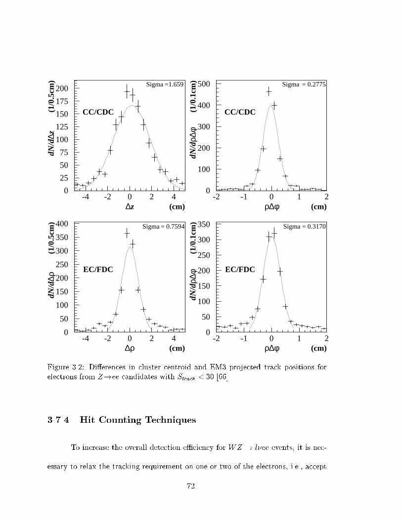
Sigma =1.659 Sigma = 0.2775

Sigma = 0.7594 Sigma = 0.3170

∆z ρ∆φ

∆ρ ρ∆φ

dN/d

∆z

dN/d

ρ∆φ

dN/d

∆ρ

dN/d

ρ∆φ

(cm) (cm)

(cm) (cm)

(1/0

.5cm

)

(1/0

.1cm

)

(1/0

.5cm

)

(1/0

.1cm

)

CC/CDC CC/CDC

EC/FDC EC/FDC

0

25

50

75

100

125

150

175

200

-4 -2 0 2 40

100

200

300

400

500

-2 -1 0 1 2

0

50

100

150

200

250

300

350

400

-4 -2 0 2 40

50

100

150

200

250

300

350

-2 -1 0 1 2

Figure 3.2: Di�erences in cluster centroid and EM3 projected track positions forelectrons from Z!ee candidates with Strack < 30 [66].

3.7.4 Hit Counting Techniques

To increase the overall detection e�ciency for WZ ! l�ee events, it is nec-

essary to relax the tracking requirement on one or two of the electrons, i.e., accept

72

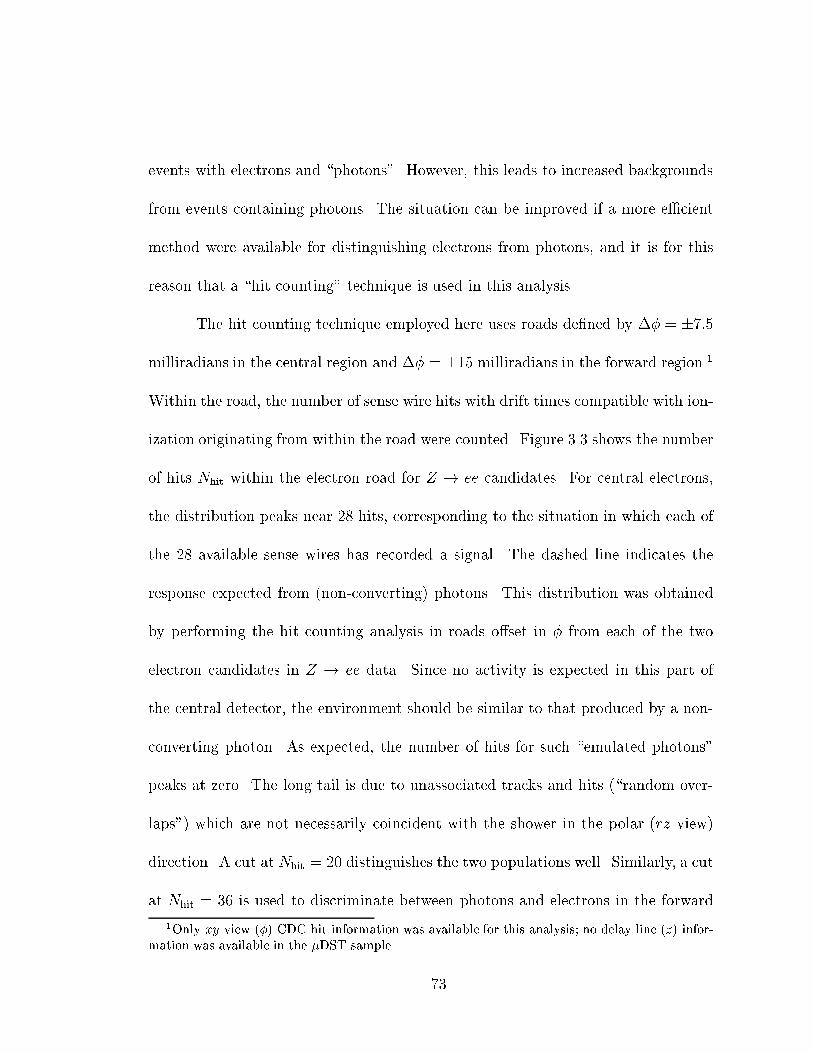
events with electrons and \photons". However, this leads to increased backgrounds

from events containing photons. The situation can be improved if a more e�cient

method were available for distinguishing electrons from photons, and it is for this

reason that a \hit counting" technique is used in this analysis.

The hit counting technique employed here uses roads de�ned by �� = �7:5

milliradians in the central region and �� = �15 milliradians in the forward region.1

Within the road, the number of sense wire hits with drift times compatible with ion-

ization originating from within the road were counted. Figure 3.3 shows the number

of hits Nhit within the electron road for Z ! ee candidates. For central electrons,

the distribution peaks near 28 hits, corresponding to the situation in which each of

the 28 available sense wires has recorded a signal. The dashed line indicates the

response expected from (non-converting) photons. This distribution was obtained

by performing the hit counting analysis in roads o�set in � from each of the two

electron candidates in Z ! ee data. Since no activity is expected in this part of

the central detector, the environment should be similar to that produced by a non-

converting photon. As expected, the number of hits for such \emulated photons"

peaks at zero. The long tail is due to unassociated tracks and hits (\random over-

laps") which are not necessarily coincident with the shower in the polar (rz view)

direction. A cut at Nhit = 20 distinguishes the two populations well. Similarly, a cut

at Nhit = 36 is used to discriminate between photons and electrons in the forward

1Only xy view (�) CDC hit information was available for this analysis; no delay line (z) infor-mation was available in the �DST sample.

73

region. The high multiplicity environment at forward angles makes this distinction

less pronounced than in the forward region.

Number of hits

Fre

quen

cy

CDC

γ e

Number of hits

FDC

γ e

0

0.05

0.1

0.15

0.2

0.25

0.3

0 10 20 30 40 500

0.02

0.04

0.06

0.08

0.1

0.12

0.14

0 50 100 150 200

Figure 3.3: Number of drift chamber hits for both Z ! ee candidates (solid) forboth the central and forward regions. The dashed line indicates the number ofrandom hits in emulated photon roads.

3.8 Muon Reconstruction

The reconstruction of muon tracks begins by turning the timing information

of a hit into a hit location. Tracks are formed from hits in B and C layer outside the

toroid and hits in the A layer inside the toroid. A trajectory is formed by matching

a BC layer track with an A layer track that matches it closely in the mid toroid

74

plane.

The momentum is determined by the angle between the A layer and BC layer

track, the �eld strength (2 T) and corrections for energy losses in the calorimeter.

A global �t for the best measured momentum is performed using the muon system

tracks, the primary interaction vertex, energy deposition in the calorimeter and a

track from the CDC(FDC) if on is present. Addition corrections are made for the

e�ects of multiple scattering in the calorimeter and the magnets.

3.9 Muon Identi�cation

O�ine identi�cation criteria must be made to select real muons from WZ

events and to reject combinatoric and cosmic ray backgrounds. The following prop-

erties of reconstructed muon candidates are used for this purpose:

� Muon Fit Quality (IFW4):

The muon reconstruction makes a number of cuts on the number of PDT

modules hit, the hit residuals, and the track impact parameters. IFW4 is the

number of cuts failed by the candidate muon. Therefore a perfect track would

have IFW4=0.

� Hadronic Fraction (HFRAC):

75

A moun will deposit energy as it passes through the calorimeter forming a

track. HFRAC is the fraction of calorimeter cells along this track in the

hadronic layers which have energy consistent with a minimum ionizing particle.

� xy Impact Parameter:

A cosmic ray muon is not likely to pass near the beam position. The xy impact

parameter is found by projecting a track into the xy plane, extrapolating

the track to the center of the detector and measuring the distance from the

primary vertex. Muons arising from the primary vertex will have a small

impact parameter.

� Floating time o�set (tfloat0 ):

The time of the hits in the track are allowed to oat in the �t. The di�erence

between the best-�t time and the beam crossing is calculated. Muons arising

from the primary vertex will have a small di�erence while out-of-time cosmic

ray muons will have a large di�erence.

� Path length in the magnet (R ~B � ~dl):

R ~B � ~dl measures the integrated magnetic �eld a muon traverses as it passes

through the iron toroid magnet. In order to measure the muon momentum

accurately, the muon must pass though a minimum �eld integral.

� Muon isolation (�R(�; jet)):

76

The muons of interest in this analysis result from W decays and are typically

well isolated from nearby particles. Muons from the semileptonic decay of

bottom and charm quarks are produced in association with hadronic particles

and are a background for this analysis. A cut in the separation of a muon

from nearby energetic jets (ET > 10 GeV) ensures that only isolated muon

are selected.

3.10 Post-RECO Corrections

3.10.1 Jet Corrections

Several corrections are made to jets after event reconstruction so that the

jet energy more closely approaches that of the originating hadron. These include

corrections for out-of-cone energy, underlying event, and low energy particles.

The energy of secondary particles may fall outside the cone used for recon-

structing the jet. The energy lost depends on the cone size used as well as the region

of the detector where the shower develops.

Low energy particles with energy of order 2 GeV produce a non-linear re-

sponse in the calorimeter cells and simple summing of cells does not account for all

energy.

Energy from the spectator quarks (those which did not interact) may be

deposited in the calorimeter and must be subtracted from the measured energy.

77

To approximate the energy of the parent particle a correction factor is needed.

This e�ect was taken into account by performing a study to determine the correc-

tion factor for jet energy as a function of jet energy and detector region [75]. This

was studied by examining the ET balance of events containing an isolated electro-

magnetic cluster (due to a photon or a jet which fragmented mostly into neutral

hadrons) and one jet, but no other objects. Any E/T in the event could be attributed

to the mismeasurement of the hadronic jet because there is no neutrino present. This

correction was coded into a standard package called CAFIX, short for calorimeter

�x.

Once these corrections have been made to the jet energies the missing energy

must be corrected to re ect these changes. Two additional versions of the missing

energy are calculated, one which is based one calorimeter energy only and another

which includes additional corrections for muons which pass quality cuts. These two

E/T calculations form the basis of the E/T calculated in this analysis (see Section

3.8.3).

3.10.2 Revertexing by Cluster-Track Projection

As mentioned earlier, the standard distinction between photons and electrons

is based on whether or not a track is found in the road de�ned by the calorimeter

cluster and the primary vertex. If the vertex position is not measured accurately,

the road de�nition is incorrect, which leads to possible misidenti�cation of electrons

78

as photons. Any kinematic quantities (ET , invariant masses, etc.) which depend

on the vertex position will be a�ected as well. The cluster-track projection method

was developed to correct this problem and is documented in Reference [76].

Cluster-track projection begins by rede�ning an electron. Instead of relying

on tracking roads to de�ne an electron, an electron is de�ned by track-cluster asso-

ciation, which is based solely on the track match signi�cance of a given track-cluster

pair. The track which is best matched to a cluster is not required to fall within the

tracking road described previously; it need only satisfy the track match signi�cance

criteria.

This best matched track is then used to unambiguously determine where

the electron originated by extrapolating the line connecting the calorimeter cluster

centroid and the drift chamber hits center of gravity to the beamline. Thus the

vertex z position, denoted zv, is given by

zv = ztrk0 � zcal0 � ztrk0

�cal0 � �trk0

!�trk0 (3.1)

where (ztrk0 ; �trk0 ) and (zcal0 ; �cal0 ) are the centroid positions of the drift chamber and

calorimeter hits, respectively. This extrapolation is shown schematically in Fig-

ure 3.4 for clarity. The track hit centroids are used since corrections to CDC delay

line biases are parameterized in terms of the centroid positions [77]. The best

matched track must satisfy the signi�cance criteria described earlier: Strack < 5 in

the central region and Strack < 10 in the forward region.

79

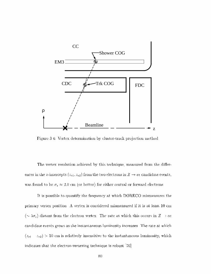
CC

CDC

EM3

FDC

Shower COG

Trk COG

z

ρ

Beamline

Figure 3.4: Vertex determination by cluster-track projection method.

The vertex resolution achieved by this technique, measured from the di�er-

ences in the z-intercepts (zv1; zv2) from the two electrons in Z ! ee candidate events,

was found to be �z � 2:0 cm (or better) for either central or forward electrons.

It is possible to quantify the frequency at which D�RECO mismeasures the

primary vertex position. A vertex is considered mismeasured if it is at least 10 cm

(� 5�z) distant from the electron vertex. The rate at which this occurs in Z ! ee

candidate events grows as the instantaneous luminosity increases. The rate at which

(zv1 � zv2) > 10 cm is relatively insensitive to the instantaneous luminosity, which

indicates that the electron-vertexing technique is robust [76].

80

3.10.3 Missing Energy Corrections

The E/T calculation for this analysis begins with the missing energy which

includes jet corrections calculated by CAFIX. The EM objects in the event are

corrected to the electron vertex determined by the cluster-track projection technique

described in the previous section using the electron closest to �det = 0 with a matched

track. The vector sum of the corrections to the electrons are subtracted from E/T .

Any jets in the event with transverse energy ET greater than 10 GeV are corrected

to the electron vertex by treating them as point-like (i.e. reclustering of the jet with

respect to the new vertex z-position is not done). The corrections to the jets are

also subtracted from E/T . The algorithm for revertexing the jets uses the average

radius of the hadronic part of the central calorimeter and the average z position of

the hadronic part of the endcap calorimeter when recalculating the jet ET . This is

done to ensure that the E/T is corrected by all calorimeter objects in the event, not

just EM objects. Correcting the E/T only for EM objects might create false E/T due

to the imbalance from not correcting the jet ET 's.

81

Chapter 4

Event Selection

4.1 Data Samples

The data samples used in this analysis was the Electroweak group's �DST

sample. The data was streamed into two samples, the W ! e� sample and the

Z ! ee sample. The Z sample was made from the 93-95 and 95-96 data samples.

TheW sample was made from 93-95 data sample only. TheW ! e� stream required

at least one EM object with ET > 15 GeV and E/T > 10 GeV; the Z ! ee stream

required at least 2 EM clusters with ET > 10 GeV.

A third diagnostic sample was created from events which �red the single

electron triggers in the 93-95 and 95-95 data samples. Data taken under this trigger

were highly prescaled because of the loose requirements of one low ET EM cluster.

In selecting l�ee (l = �; e) candidates, bad runs were excluded. These bad

82

runs had known calorimeter or tracking problems. Runs where the luminosity was

unknown were also rejected.

In the �nal analysis the data sample used to select WZ ! l�ee events was

the Z sample because of the higher available luminosity. The W sample was used

only as a cross check.

4.2 Luminosity

The GET FILT LUM utility was used to obtain the integrated luminos-

ity of the streamed data sets for the Level-2 �lters used in this analysis. The

GET FILT LUM utility takes into account any any active veto scheme that was

present in the trigger, as well as any prescales that were applied. After applying the

GOODBEAM requirement o�ine, the integrated luminosity was found to be 92.3

pb�1 . The e�ciency of the o�ine GOODBEAM cut was estimated by counting the

number of events before and after the GOODBEAM cut. The error in the integrated

luminosity introduced by this estimate is 0.7%. A 5.4% systematic uncertainty is

assigned to the integrated luminosity as determined from the luminosity database.

The two errors added in quadrature gives an error of 5.4% on the luminosity. The

�nal integrated luminosity for the l�ee analysis is therefore L = (92:3� 5:0)pb�1.

83

4.3 Trigger

The Level-2 trigger used in this analysis, EM2 EIS2 HI, is described below:

� Level-0 trigger (hardware)

{ The universal Level-0 minimum bias requirement was imposed through-

out the data taking period: this consisted of the detection of an inelastic

collision with simultaneous hits in the north and south Level-0 counters,

as well as a fast z determination with jzj < 100 cm.

� Level-1 trigger (hardware)

{ 2 EM objects with EEMT > 7:0 GeV;

{ events occurring in the MRBS LOSS and MICROBLANK periods simul-

taneously were rejected.

� Level-1.5 trigger (hardware)

{ 2 EM objects with EEMT > 12:0 GeV

{ and with EM fraction > 0:85.

� Level-2 �lter (software)

{ 2 EM objects with ET > 20:0 GeV;

{ Loose shower shape and isolation cuts on both objects.

84

4.4 O�ine Electron Selection

For this analysis electrons are classi�ed as \loose" or \tight" electrons with

the tight electrons being a subset of the loose electrons. A loose or tight electron

must fall within a �ducial volume where electrons can be well measured. This

excludes the regions between the CC and EC cyrostats, 1:1 < j�detj < 1:5, where

the electron identi�cation e�ciency is poor, the very forward regions of the detector

where the segmentation of the EM calorimeter decreases, j�detj > 2:5, the edge of the

CDC where the tracking e�ciency drops, 1:0 < j�detj < 1:1, and the gaps between

the 32 modules of the �rst layer of the central electromagnetic calorimeter (CCEM).

The �ducial region for loose and tight electrons is then de�ned as:

� Central Calorimeter (CC): j�detj < 1:0 and j��(cluster,crack)j > 0:01

��(cluster,crack) is the separation between the shower centroid and the bound-

aries of the �rst layer of EM modules which occur at � = 2n�32, n=0 to 31.

� Endcap Calorimeter (EC): 1:5 < j�detj < 2:5

Loose and tight electrons are required to pass shower shape and isolation

cuts. A tight electron is required to have a matching track and a loose electron is

required to have either a matching track or hits in the drift chamber along a � road

between the EM cluster centroid and the z axis.

The criteria for loose and tight electrons are:

85

� Tight Electron

{ Isolation I < 0:10

{ Shower shape covariance parameter

�2 < 100 in the CC

�2 < 200 in the EC

{ A matching track with signi�cance

Strack < 5 in the CDC

Strack < 10 in the FDC

� Loose Electron

{ Isolation, I < 0:10

{ H-matrix �2 < 100; 200 (CC, EC)

{ Number of hits on drift chamber wires NHxy > 20, 36 (CDC, FDC)

or a matching track with signi�cance Strack < 5; 10 (CDC, FDC)

The choice of the tracking cuts for the electrons was motivated by the need

to maintain high e�ciency. In this analysis we used relatively loose electron iden-

ti�cation cuts since the backgrounds are small. Two variables used in electron

identi�cation, the dE/dx and TRD information, were not used in this analysis to

maintain high e�ciency. The explicit track requirement was dropped for loose elec-

trons because some tracks are not reconstructed in a high luminosity environment.

86

4.5 O�ine Muon Selection

The following quality cuts were used to select the muon:

� j�j < 1:0

� Muon �t quality IFW4�1

� Hadronic fraction HFRAC�0.70

� jxy impact parameterj � 25 cm

� Floating time o�set (jtfloat0 j) � 200 ns

� Field IntegralR ~B � ~dl � 0:6 GeV

� Isolation �R(�; jet) � 0:5 for EjetT > 10 GeV

The �rst cut allows only muons in the CF region, eliminating punch-through

and combinatoric backgrounds. The second cut is on the quality of the muon track

�t. The third cut is used to ensure that the muon deposits energy in its passage

through the calorimeter, thus rejecting fake muon tracks due to noise hits. The

fourth and �fth cuts are used to reject cosmic muons, which do not necessarily pass

near the beam line and which arrive out of time with the beam crossing.

87

4.6 WZ ! e�ee event selection.

WZ ! e�ee events are characterized by three high-ET electrons and large

E/T . The following cuts are used to select events:

� Events occurring in the MRBS LOSS or MICROBLANK periods are rejected

� Events must pass the EM2 EIS2 HI trigger;

� One tight electron with ET > 25, one loose electron with ET > 25 GeV and

one loose electron with ET > 10 GeV ;

The cut on the �rst two electrons is chosen so that the trigger e�ciency is

greater than 98%. The cut on the third electron, which is assumed not to

be one of the trigger electrons, is allowed to be as loose as practical. The

tight electron is used to de�ne the vertex using the cluster-track projection

technique. If two or more tight electrons are found, the central most (smallest

j�detj) electron is used to de�ne the vertex.

� E/T > 15 GeV

This is the E/T corrected for the changes in electron and jet ET due to rever-

texing.

� Events with invariant and transverse mass consistent with the Z and W are

selected.

88

The transverse mass of electron k and the E/T must be greater than 30 GeV/c2

and the invariant mass of electron i and j is between 81 and 101 GeV/c2, i.e.

mT (k; E/T ) > 30GeV=c2

where

m2T = 2Ee

TE/T (1� cos(�e � ��))

and

81GeV=c2 < mi;j < 101GeV=c2

These cuts are checked for all three combinations of electrons i, j, and k.

If more than one combination passes the cut, the combination with the Z

mass closest to 91 GeV is used. This cut along with the E/T cut is used to

reject background from two electron plus one jet events where the jet fakes an

electron.

After applying all the event selection cuts one event is selected. The proper-

ties of the event are summarized in Appendix A. This event has two reconstructed

vertices at z = �23 and +25 cm. One high ET electron and two high ET photons

are identi�ed by the reconstruction program using the vertex at �23 cm as shown

in Figure 4.1. The end view of the calorimeter and tracking is shown in Figure 4.2.

Upon revertexing, a track pointing towards the vertex at +25 cm is matched to one

of the photons identifying it as a tight electron. The electron also has a track point-

ing towards the vertex at +25 cm. The second \photon" has hits in a road pointing

89

towards the vertex at +25 cm. Revertexing the event using the two tight electrons

yields a vertex z position of +25:5 cm. The two tight electrons form an invariant

mass of 93.6 GeV/c2 and have a di-electron transverse momentum of 58.8 GeV/c.

The loose electron and the corrected missing transverse energy form a transverse

mass of 74.7 GeV/c2 with a transverse momentum of 63.0 GeV/c.

4.7 WZ ! ��ee event selection

WZ ! ��ee events are characterized by two high-ET electrons, a high pT

muon, and large E/T . The following cuts were used to select events:

� Events within the MRBS LOSS and MICRO BLANK gate are rejected;

� Events must pass the EM2 EIS2 HI trigger;

� Events must have one tight electron with ET > 25, one loose electron with

ET > 25 GeV and one muon with pT > 15 GeV ;

� Events must have muon-corrected and calorimeter missing transverse energy

E/T > 15 GeV.

The calorimeter missing energy cut ensures that the missing energy is real and not

just an artifact of a mismeasured muon. No events are observed with this minimal

set of cuts.

90

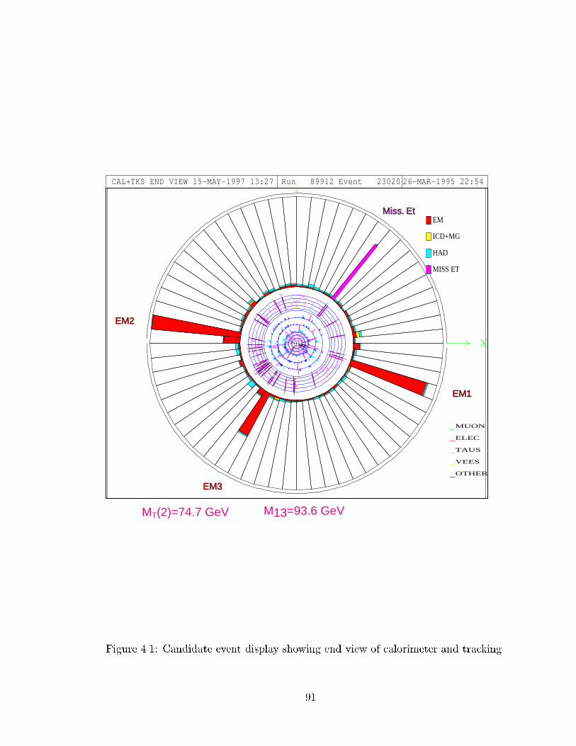
CAL+TKS END VIEW 15-MAY-1997 13:27 Run 89912 Event 23020 26-MAR-1995 22:54

.......

......

...........

.........

.........

.........

.

.

.

.

.

.

.

.

.

.

.

.

.

...............

..........

....

....

...

....

....

... ......

.....................

.............

..............

.......

.......

............

..............

....................

.......

.

............

......

.....................

....

....

..

...

... .

... .

... .

..

....... ...... ...................

...........

......

......

...........

...

...

..

.......

.....

...

...

...

...

...

.......

.

.............

.....

.....

.....

.....

.....

....

.... .......

.....................

..... ....................

...................

.....

............

..............

...................

.

............

.

.

.....

..

..

..

..

.

..... ...

....

....

.........

............ ....... ....... ..............

..............

MUON

ELEC

TAUS

VEES

OTHER

EM

ICD+MG

HAD

MISS ET

EM2

EM3

EM1

Miss. Et

MT(2)=74.7 GeV M13=93.6 GeV

Figure 4.1: Candidate event display showing end view of calorimeter and tracking.

91

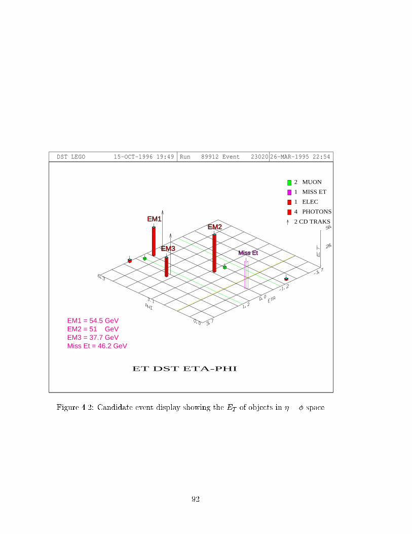
DST LEGO 15-OCT-1996 19:49 Run 89912 Event 23020 26-MAR-1995 22:54

ET DST ETA-PHI

2 MUON

1 MISS ET

1 ELEC

4 PHOTONS

2 CD TRAKS

EM1 = 54.5 GeVEM2 = 51 GeVEM3 = 37.7 GeVMiss Et = 46.2 GeV

EM1EM1

EM3EM3

EM2EM2

Miss Et

Figure 4.2: Candidate event display showing the ET of objects in � � � space.

92

Chapter 5

Detection E�ciencies

Not all events produced in a collision will be recorded by the detector. Events

might not �re a hardware or software trigger and the event might not pass the

particle identi�cation criteria. In order to estimate this loss, the e�ciencies of the

trigger and the o�ine particle identi�cation criterion must be determined.

5.1 Trigger E�ciency

To estimate the loss of events that do not �re a trigger, a trigger e�ciency

needs to be determined. Ideally the trigger e�ciency would be obtained from the ra-

tio of the number of events passing the EM2 EIS2 HI trigger to events selected with

no trigger requirement. A more practical method is to evaluate the trigger e�ciency

for an electron to pass the Level 2 trigger requirements using data selected with a

93

trigger with looser requirements than the EM2 EIS2 HI trigger. Data taken with

the EM2 ELE ESC trigger had the same Level-1 requirement as the EM2 EIS2 HI

trigger, but a looser ET requirement (16 GeV) and no isolation or shape require-

ments, and are therefore unbiased with respect to the EM2 EIS2 HI trigger. The

Level-2 e�ciency for ET > 20 GeV can be measured using coincidences of the two

�lters in Z ! ee data. The fraction of events in each ET bin which satis�ed the

level-2 ET > 20 GeV is a measure of the ET dependence of the e�ciency of the

Level-2 requirement. The resulting e�ciency turn on curve is shown in Figure 5.1.

A cut of 25 GeV yields a trigger e�ciency of greater than 98% per electron for CC

or EC electrons.

5.2 Electron Identi�cation E�ciencies

To estimate the loss of events that do not pass the o�ine particle identi-

�cation criteria described in Chapter 4, an ID e�ciency needs to be determined.

The e�ciency of ID cuts are determined using Z ! ee events as described in Ref-

erence [76] for the 93-95 and 95-96 data samples. The change in the number of

events in the Z mass window for di�erent cuts allows a relative e�ciency to be de-

termined. Backgrounds are subtracted from the Z-mass windows using two methods

and two mass windows. The �rst method uses sideband averaging to determine the

background in the Z mass window. The second method �ts the di-electron mass

94

distribution to a Breit-Weigner distribution convoluted with a Gaussian distribution

plus a linear background and subtracts the linear background from the Z mass peak.

The mass windows used were of width 10 GeV and 20 GeV centered on the Z mass

of 91 GeV.

The relative e�ciency of cut \a" relative to some looser cut \b" is given by

�ab = Sab=Sb

where Sab and Sb denote the number of background-subtracted events in the mass

peak after background subtraction for cuts \a" and \b" together and cut b alone,

respectively. Using the two methods with the two mass windows, four estimates of

the e�ciency are obtained. The e�ciency is taken to be the average of the four

methods. Errors are calculated using the binomial error on the ratios added in

quadrature with the largest di�erence between the average and the four e�ciencies.

Table 5.1 lists the e�ciencies obtained in this manner for both the forward and

central regions. The quantities �t and �l in Table 5.1 are the identi�cation e�ciencies

for tight and loose electrons, respectively. The e�ciency for the calorimeter-based

cuts (I; �2) is denoted �cal, the e�ciency for track reconstruction is denoted �trk, and

the e�ciency for a track or hit requirement is denoted �hit. With these de�nitions,

�t ' �cal�trk and �l ' �cal�hit.

The e�ciencies for the isolation and shower shape requirements are valid for

high ET electrons and photons. However, corrections must be made at low ET .

95

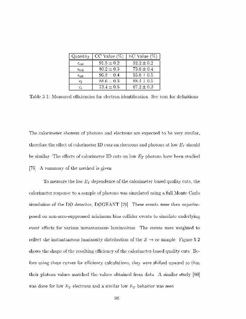
Quantity CC Value (%) EC Value (%)

�cal 91:5� 0:2 92:2� 0:2�trk 80:2� 0:3 73:8� 0:4�hit 96:8� 0:4 95:8� 0:5�l 88:6� 0:3 88:4� 0:5�t 73:4� 0:5 67:2� 0:3

Table 5.1: Measured e�ciencies for electron identi�cation. See text for de�nitions.

The calorimeter showers of photons and electrons are expected to be very similar,

therefore the e�ect of calorimeter ID cuts on electrons and photons at low ET should

be similar. The e�ects of calorimeter ID cuts on low ET photons have been studied

[76]. A summary of the method is given.

To measure the low ET dependence of the calorimeter-based quality cuts, the

calorimeter response to a sample of photons was simulated using a full Monte Carlo

simulation of the D� detector, D�GEANT [79]. These events were then superim-

posed on non-zero-suppressed minimum bias collider events to simulate underlying

event e�ects for various instantaneous luminosities. The events were weighted to

re ect the instantaneous luminosity distribution of the Z ! ee sample. Figure 5.2

shows the shape of the resulting e�ciency of the calorimeter-based quality cuts. Be-

fore using these curves for e�ciency calculations, they were shifted upward so that

their plateau values matched the values obtained from data. A similar study [80]

was done for low ET electrons and a similar low ET behavior was seen.

96

To determine if there is an ET dependence for the tracking variable e�cien-

cies, events selected with the EM2 ELE ESC trigger, which contained electrons with

ET � 16 GeV, were used. Within errors, the track match and hits cut e�ciency

relative to the calorimeter cuts are the same for high ET and low ET electrons.

Therefore no ET dependence is assigned to the tracking e�ciencies. The e�ciency

of the track match cut relative to the calorimeter cuts in these events was found to

be 80:4� 0:2(sys)� 0:5(stat)% for the CDC and 72:6� 0:4(sys)� 0:8(stat)% for the

FDC. The e�ciency of the hits cut relative to the calorimeter cuts was found to be

97:1 � 0:2(sys) � 0:2(stat)% for the CDC and 95:3 � 0:2(sys) � 0:4(stat)% for the

FDC.

5.3 Muon Identi�cation E�ciencies

Since the muon identi�cation criteria used in this analysis are identical to

those used in the D� WW ! l�l0� 0 analysis [81, 82] of the 93-95 data sample, we

use the e�ciencies calculated in that analysis, which are detailed in Reference [81].

The e�ciencies for each cut were determined from a combination of Monte Carlo

and data. The e�ciencies for the IFW4 andR ~B � ~dl cuts as a function of � � �

were determined from D�GEANT events, and the e�ciencies of the remaining cuts

were determined from data. The e�ciency of each cut, except the IFW4 andR ~B � ~dl

cut, was determined using Z ! �� events. The overall e�ciency for muons with

97

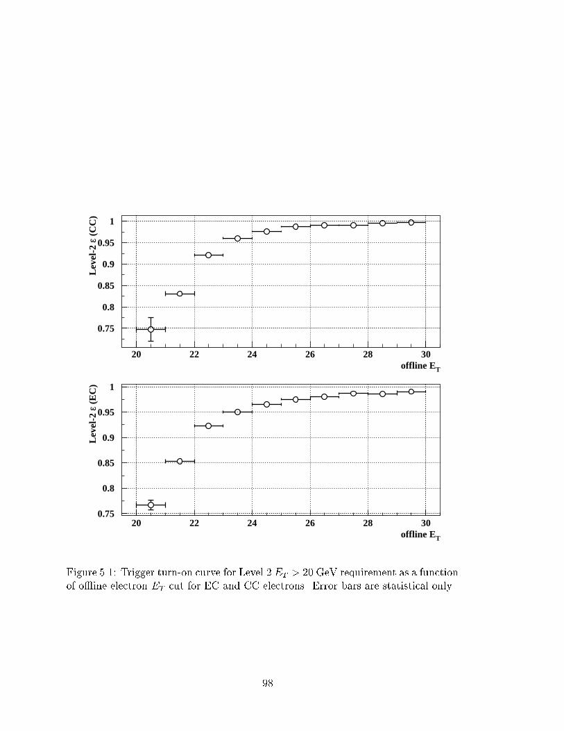
0.75

0.8

0.85

0.9

0.95

1

20 22 24 26 28 30offline ET

Leve

l-2 ε

(CC

)

0.75

0.8

0.85

0.9

0.95

1

20 22 24 26 28 30offline ET

Leve

l-2 ε

(EC

)

Figure 5.1: Trigger turn-on curve for Level 2 ET > 20 GeV requirement as a functionof o�ine electron ET cut for EC and CC electrons. Error bars are statistical only.

98

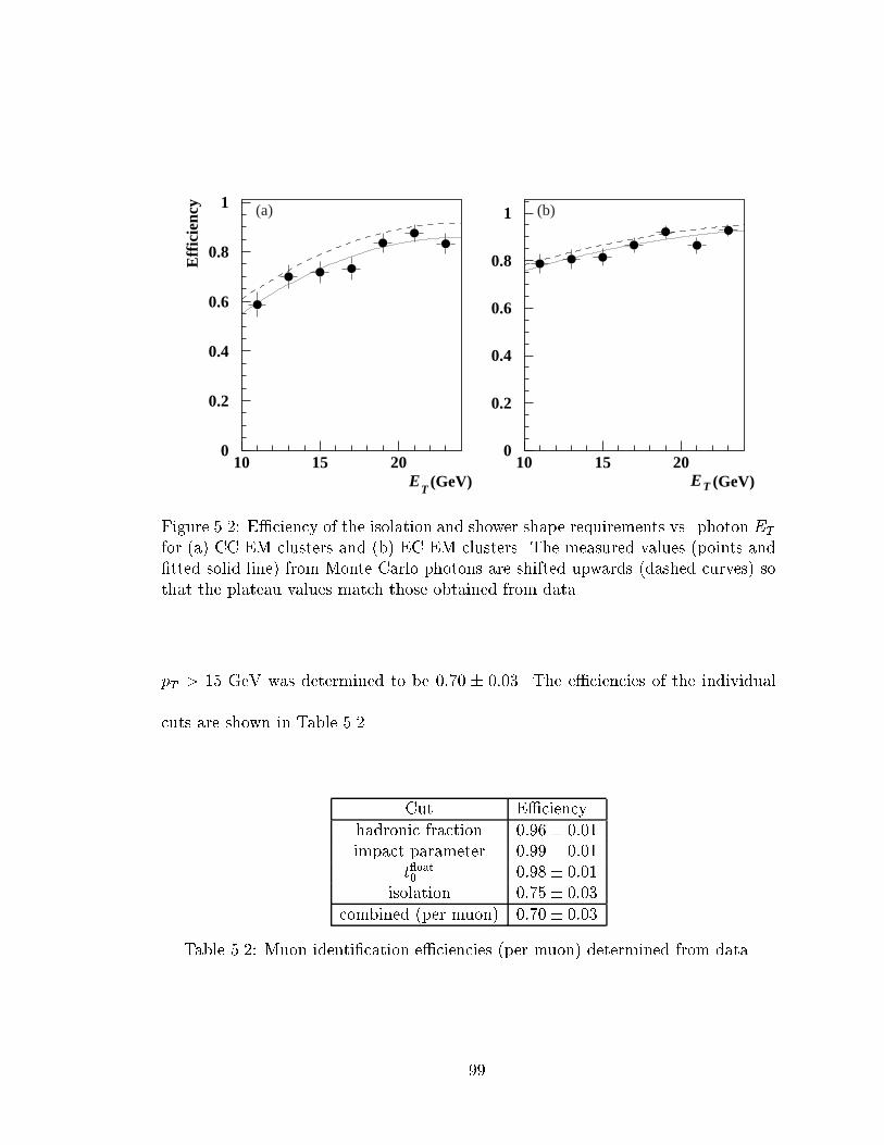
ET

(GeV)

Effi

cien

cy

ET (GeV)

0

0.2

0.4

0.6

0.8

1

10 15 200

0.2

0.4

0.6

0.8

1

10 15 20

(a) (b)

Figure 5.2: E�ciency of the isolation and shower shape requirements vs. photon ET

for (a) CC EM clusters and (b) EC EM clusters. The measured values (points and�tted solid line) from Monte Carlo photons are shifted upwards (dashed curves) sothat the plateau values match those obtained from data.

pT > 15 GeV was determined to be 0:70 � 0:03. The e�ciencies of the individual

cuts are shown in Table 5.2

Cut E�ciencyhadronic fraction 0:96� 0:01impact parameter 0:99� 0:01

t oat0 0:98� 0:01isolation 0:75� 0:03

combined (per muon) 0:70� 0:03

Table 5.2: Muon identi�cation e�ciencies (per muon) determined from data.

99

Chapter 6

Signal Event Simulation

The number of events predicted is determined by multiplying the theoreti-

cal cross section by the integrated luminosity. However, to determine the number

of events visible in the detector it is necessary to simulate the response of the de-

tector and the o�ine reconstruction and event selection. A detection e�ciency is

determined from this simulation. The number of events seen is then the number of

predicted events multiplied by the detection e�ciency.

6.1 Monte Carlo Event Generator

The leading order Monte Carlo event generator of Zeppenfeld, et al. [9] was

used to calculate the WZ production cross section as a function of the WWZ cou-

plings and to obtain distributions of various kinematic variables. The cross section

100

calculated by this program includes multiplication by a \K-factor" equal to 1.335

to take into account the e�ects of higher order QCD corrections. The program was

modi�ed to output the 4-vectors of the �nal state particles for input to the detector

simulation described below.

The Zeppenfeld Monte Carlo event generator does not take into account the

e�ects of initial state radiation (ISR), which give rise to a signi�cant transverse mo-

mentum of the WZ system. Therefore, Standard model WZ events were generated

using PYTHIA [8] to determine the transverse momentum distribution of the WZ

system. The e�ects of ISR are included in this event generator and the resulting

pT distribution of the WZ system is plotted in Figure 6.2. The cross section times

branching ratio as calculated by PYTHIA is

�(p�p!WZ +X)�B(W ! l�)� B(Z ! l+l�) = 7:9 fb:

This agrees with the cross section calculated by the Zeppenfeld Monte Carlo, 10.3 fb,

once the \K-factor" is taken into account.

6.2 Detector Simulation

A large number of events need to be run through a detector simulator in

order to calculate detection e�ciencies for non Standard Model values of the WWZ

couplings. Since a full detector simulation such as GEANT [79] takes a large amount

of CPU time, a fast detector simulator, called DIPS [83], was developed by the D�

101

diboson physics group which parameterizes the detector response and can be used

to quickly calculate the detector e�ciency.

The fast detector simulator takes the following e�ects into account:

� electrons and photons energies are smeared according to the observed resolu-

tion of the electromagnetic calorimeter

��EE

�2= C2 +

S2

E+N2

E2

where E is the energy of the electron, C is the calibration error term , S is

the sampling uctuation term, and N is the noise term. The sampling term

is taken from data and the noise and calibration terms were tuned to match

those obtained from Z ! ee events which were simulated with D�GEANT

and overlaid with minimum bias collider data [76].

� muon momentum is smeared according to the resolution function

(�1=p(1=p)

)2 = (a(p� p0)=p)2 + (bp)2

where a, b, and p0 are determined from data [84].

� the primary vertex z position is smeared using a Gaussian distribution with

mean 0 and width 29 cm, and the 4-vectors are projected from that location;

� the missing energy distribution from minimum bias events is added to the ex-

isting missing energy to simulate the e�ect of underlying events on the missing

energy measurement (see Figure 6.1);

102

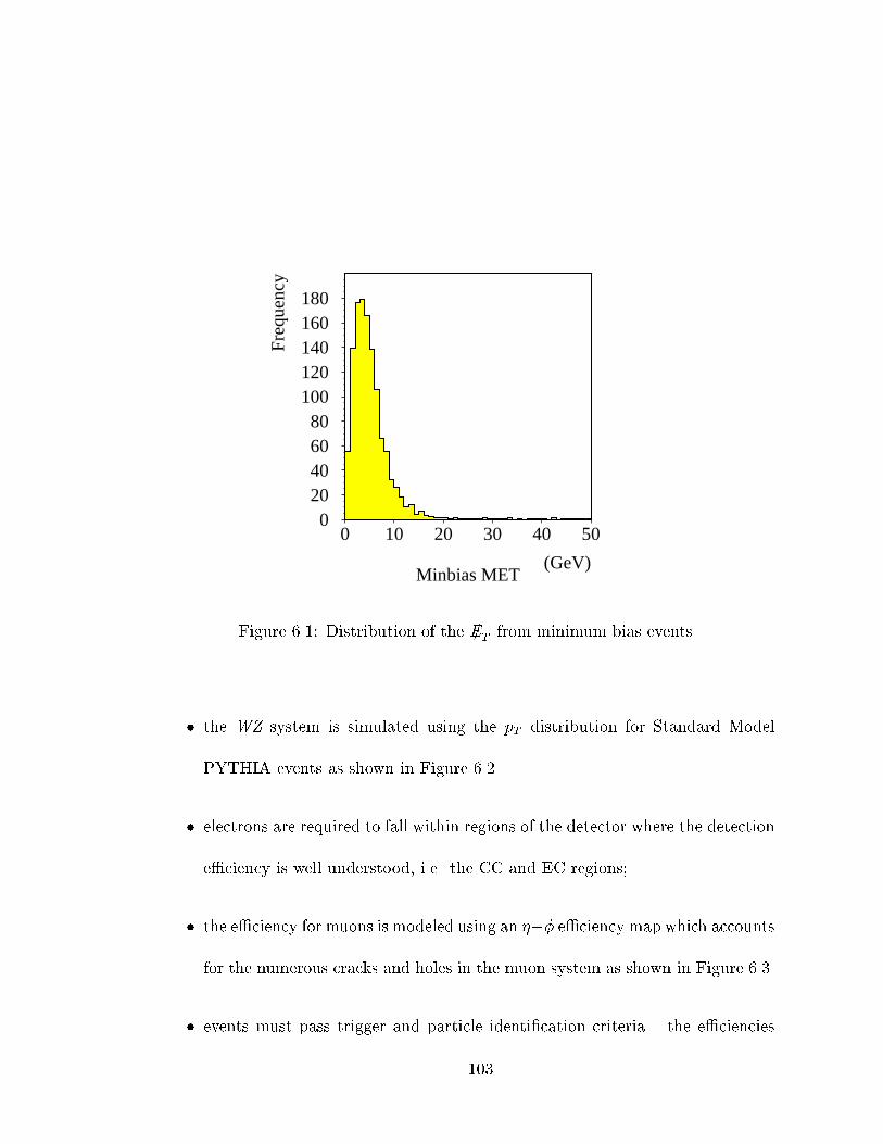
Minbias MET(GeV)

Fre

quen

cy

020406080

100120140160180

0 10 20 30 40 50

Figure 6.1: Distribution of the E/T from minimum bias events.

� the WZ system is simulated using the pT distribution for Standard Model

PYTHIA events as shown in Figure 6.2.

� electrons are required to fall within regions of the detector where the detection

e�ciency is well understood, i.e. the CC and EC regions;

� the e�ciency for muons is modeled using an ��� e�ciency map which accounts

for the numerous cracks and holes in the muon system as shown in Figure 6.3.

� events must pass trigger and particle identi�cation criteria { the e�ciencies

103

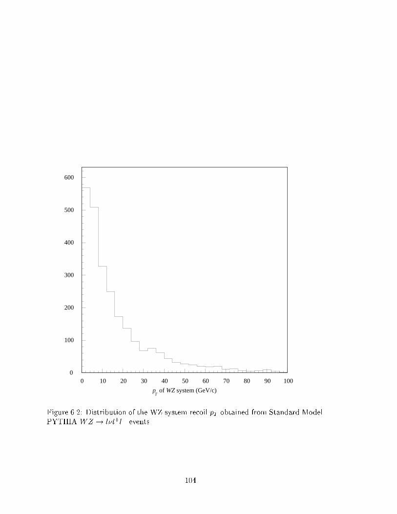
of WZ system (GeV/c)

0

100

200

300

400

500

600

0 10 20 30 40 50 60 70 80 90 100

pT

Figure 6.2: Distribution of the WZ system recoil pT obtained from Standard ModelPYTHIA WZ ! l�l+l� events.

104

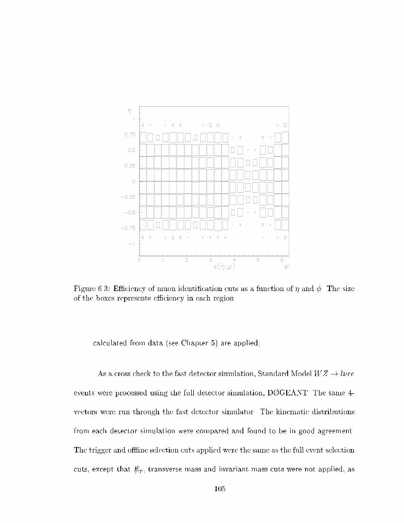
Figure 6.3: E�ciency of muon identi�cation cuts as a function of � and �. The sizeof the boxes represents e�ciency in each region.

calculated from data (see Chapter 5) are applied;

As a cross check to the fast detector simulation, Standard ModelWZ ! l�ee

events were processed using the full detector simulation, D�GEANT. The same 4-

vectors were run through the fast detector simulator. The kinematic distributions

from each detector simulation were compared and found to be in good agreement.

The trigger and o�ine selection cuts applied were the same as the full event selection

cuts, except that E/T , transverse mass and invariant mass cuts were not applied, as

105

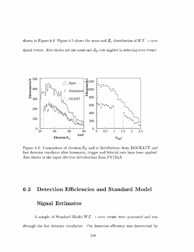
shown in Figure 6.4. Figure 6.5 shows the mass and E/T distribution of WZ ! e�ee

signal events. Also shown are the mass and E/T cuts applied in selecting e�ee events.

Electron ET

0

100

200

300

400

500

20 40 60 80GeV

Ele

ctro

ns/G

eV

|ηdet|

0

200

400

600

800

1000

1200

0 0.5 1 1.5 2 2.5

Ele

ctro

ns/0

.1Input

Simulation

GEANT

Figure 6.4: Comparison of electron ET and � distributions from D�GEANT andfast detector simulator after kinematic, trigger and �ducial cuts have been applied.Also shown is the input electron distributions from PYTHIA.

6.3 Detection E�ciencies and Standard Model

Signal Estimates

A sample of Standard Model WZ ! e�ee events were generated and run

through the fast detector simulation. The detection e�ciency was determined by

106

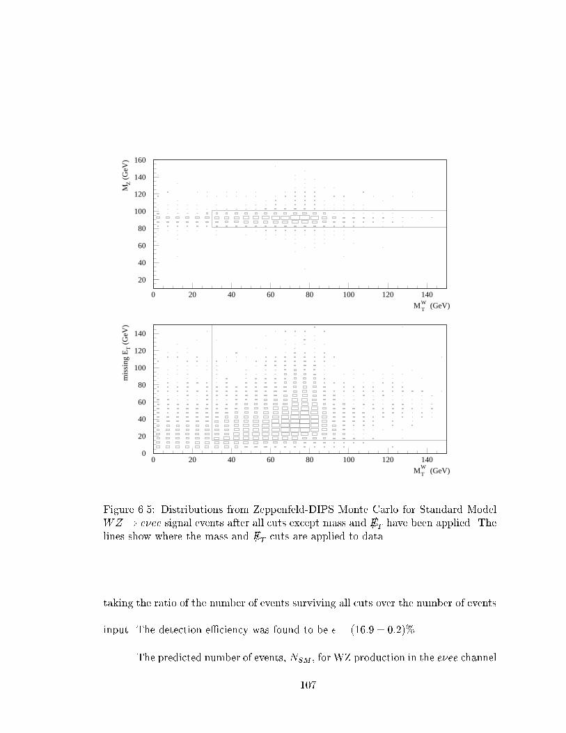
20

40

60

80

100

120

140

160

0 20 40 60 80 100 120 140

MTW (GeV)

MZ (

GeV

)

0

20

40

60

80

100

120

140

0 20 40 60 80 100 120 140

MTW

(GeV)

mis

sing

ET (

GeV

)

Figure 6.5: Distributions from Zeppenfeld-DIPS Monte Carlo for Standard ModelWZ ! e�ee signal events after all cuts except mass and E/T have been applied. Thelines show where the mass and E/T cuts are applied to data.

taking the ratio of the number of events surviving all cuts over the number of events

input. The detection e�ciency was found to be � = (16:9� 0:2)%.

The predicted number of events, NSM , for WZ production in the e�ee channel

107

is given by

NSM = � � �SM � L

where � = (16:9�0:2)% is the overall detection e�ciency, �SM = 0:0094�0:0005 pb

is the Standard Model cross section from the Zeppenfeld Monte Carlo, andR Ldt =

92:3�5:0 pb�1 is the integrated luminosity. This gives NSM = 0:146�0:002 (stat)�

0:012 (syst).

The statistical error is the error on the overall detection e�ciency which is

limited by Monte Carlo statistics. The systematic error includes the uncertainty

on integrated luminosity, particle identi�cation e�ciency, trigger e�ciency, and the

uncertainty in the Monte Carlo cross section due to choice of parton distribution

function (PDF) and momentum transfer (Q2) scale. The uncertainty on the Monte

Carlo cross section was found by varying the PDF and Q2 scale and taking the

average of the di�erences from the cross section calculated using the MRSD�0 PDF.

These errors are summarized in Table 6.1 and added in quadrature to give an overall

systematic uncertainty of 8.5% in the e�ee channel.

In the WZ ! ��ee channel, the e�ciency for detecting SM events was

determined to be (11:5 � 0:15)%. Using the same integrated luminosity and cross

section as the e�ee channel, the Standard Model expectation for the ��ee channel

is 0:099� 0:001 (stat) � 0:009 (syst) events.

108

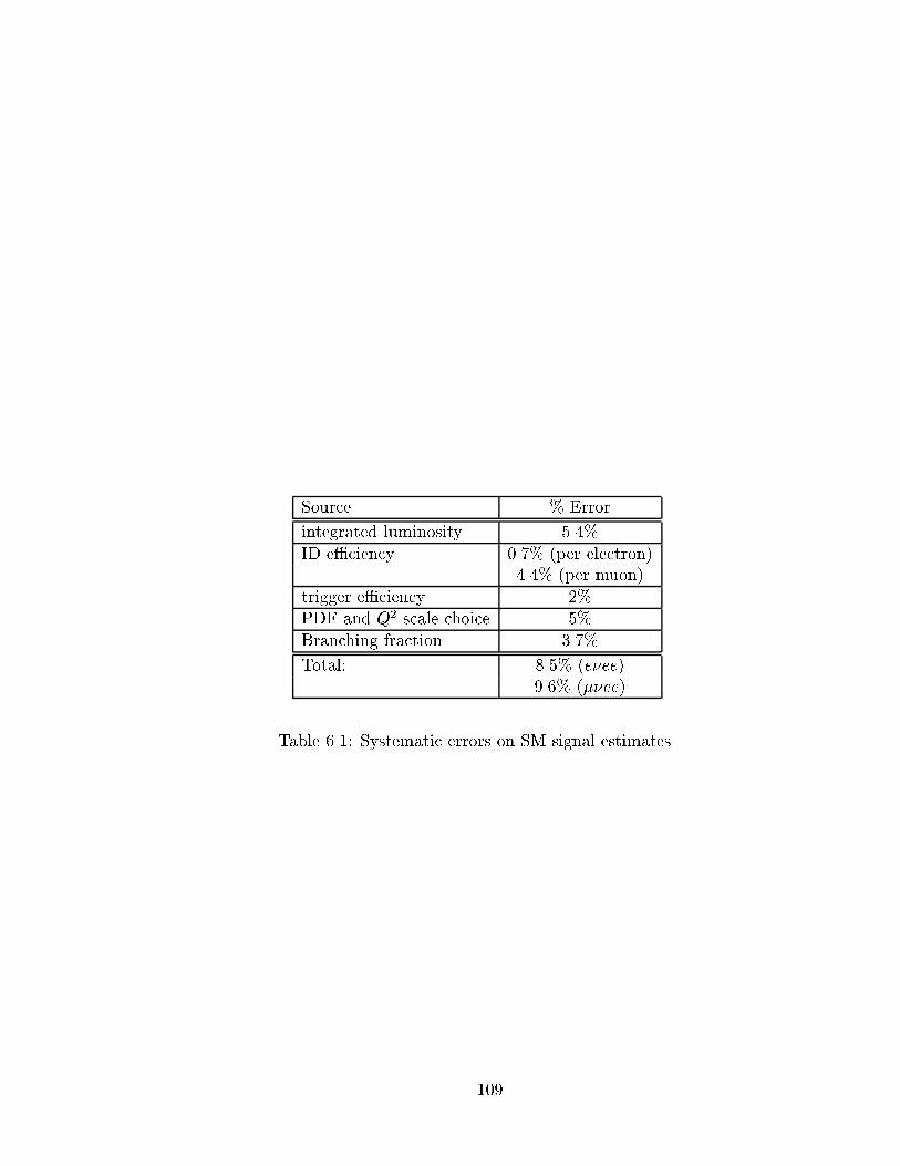
Source % Error

integrated luminosity 5.4%ID e�ciency 0.7% (per electron)

4.4% (per muon)trigger e�ciency 2%PDF and Q2 scale choice 5%Branching fraction 3.7%

Total: 8.5% (e�ee)9.6% (��ee)

Table 6.1: Systematic errors on SM signal estimates.

109

Chapter 7

Backgrounds

7.1 Backgrounds for the WZ ! e�ee Channel

The physics backgrounds for this channel are negligible because of the high

ET cuts and the high E/T cut. The backgrounds for this analysis come from a jet

faking the signature of an electron. It is possible for a jet to form a �0 or � which

then decays into . If the �0 has su�cient ET the two photons will produce a

electromagnetic shower which mimics that of an electron. If a low ET charged

hadron from the remainder of the jet or from the underlying event leaves hits in

the drift chamber, the resulting hits + cluster might pass the electron identi�cation

cuts. Another background comes from a photon converting to an e+e� pair, which

would be detected as one electromagnetic shower.

The largest background is expected to be from ee + jet events which acquire

110

their missing energy from the underlying event and the mismeasurement of the jet

energy. A Monte Carlo simulation of these events would not take this e�ect into

account, and therefore a data-based technique is used to estimate these backgrounds.

Two methods used to determine the background are described below. In

the �rst method, the number of ee + jet events which pass all event selection cuts

except that a jet is required instead of the third electron is counted and this number

is multiplied by the probability of a jet faking an electron. In the second method,

the number of events which pass all event cuts except that one electron fails the

shower shape or isolation cut is counted. This number is then multiplied by the

probability that a bad quality electron fakes a good quality electron. These events

already contain three electromagnetic clusters and are more likely to fake the event

signature than ee + jet events. This method is used as a cross check to the �rst but

has poorer statistics because of the smaller number of events.

7.1.1 Background Estimate { Method 1

The ee + jet background is calculated from the same sample as the signal.

Events must pass the EM2 EIS2 HI �lter, have two electrons (tight or loose), one or

more jets, and E/T � 15. Events are classi�ed according to the following categories:

1. TLJ { one tight electron and one loose electron both with ET � 25 and a jet

with ET � 10.

111

2. TJL� { one tight electron with ET � 25, one loose electron with ET � 10 and

a jet with ET � 25

3. JLL� { one loose electron and ET � 25, one loose electron with ET � 10

and a jet with ET � 25. Because a tight electron can be counted as a loose

electron only events where the �rst loose electron has no matching track are

accepted to avoid double counting events in category 2.

In an event where a jet fakes one of the high ET electrons and the second

electron has ET < 30 GeV the event might not pass the EM2 EIS2 HI trigger. The

event was counted if it passes one of the single electron monitor triggers. Since the

single electron triggers were prescaled with respect to the EM2 EIS2 HI trigger, a

normalization of 9:7� 0:5 was applied to the number of events under these triggers.

This normalization was based on the number of Z ! ee events which �re both

triggers.

The kinematic distributions of these ee + jet events before the mass and E/T

cuts are shown in Fig. 7.1 for events passing the EM2 EIS2 HI trigger.

The number of fake background events is found by summing the ET depen-

dent probability for all events which pass all event cuts, i.e.

Nbkg =NevtXi=1

wi(NjetsXj=1

Pj(ET ))

where Nbkg is the number of background events, Nevt is the number of ee + jet events

passing all event cuts, wi is the appropriate scaling factor for the trigger passed, Njet

112

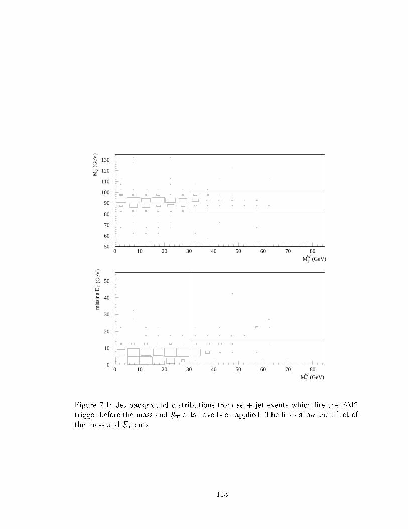
50

60

70

80

90

100

110

120

130

0 10 20 30 40 50 60 70 80

MTW (GeV)

MZ (

GeV

)

0

10

20

30

40

50

0 10 20 30 40 50 60 70 80

MTW (GeV)

mis

sing

ET (

GeV

)

Figure 7.1: Jet background distributions from ee + jet events which �re the EM2trigger before the mass and E/T cuts have been applied. The lines show the e�ect ofthe mass and E/T cuts.

113

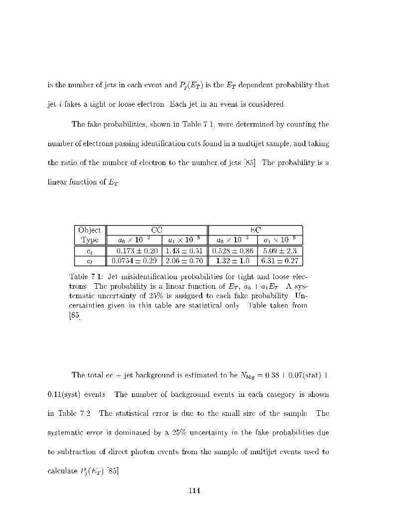
is the number of jets in each event and Pj(ET ) is the ET dependent probability that

jet i fakes a tight or loose electron. Each jet in an event is considered.

The fake probabilities, shown in Table 7.1, were determined by counting the

number of electrons passing identi�cation cuts found in a multijet sample, and taking

the ratio of the number of electron to the number of jets [85]. The probability is a

linear function of ET .

Object CC ECType a0 � 10�3 a1 � 10�5 a0 � 10�3 a1 � 10�5

et �0:173� 0:20 1:43� 0:51 0:528� 0:86 5:09� 2:3el 0:0754� 0:29 2:06� 0:70 1:32� 1:0 6:31� 0:27

Table 7.1: Jet misidenti�cation probabilities for tight and loose elec-trons. The probability is a linear function of ET , a0 + a1ET . A sys-tematic uncertainty of 25% is assigned to each fake probability. Un-certainties given in this table are statistical only. Table taken from[85].

The total ee + jet background is estimated to be Nbkg = 0:38� 0:07(stat)�

0:11(syst) events. The number of background events in each category is shown

in Table 7.2. The statistical error is due to the small size of the sample. The

systematic error is dominated by a 25% uncertainty in the fake probabilities due

to subtraction of direct photon events from the sample of multijet events used to

calculate Pj(ET ) [85].

114

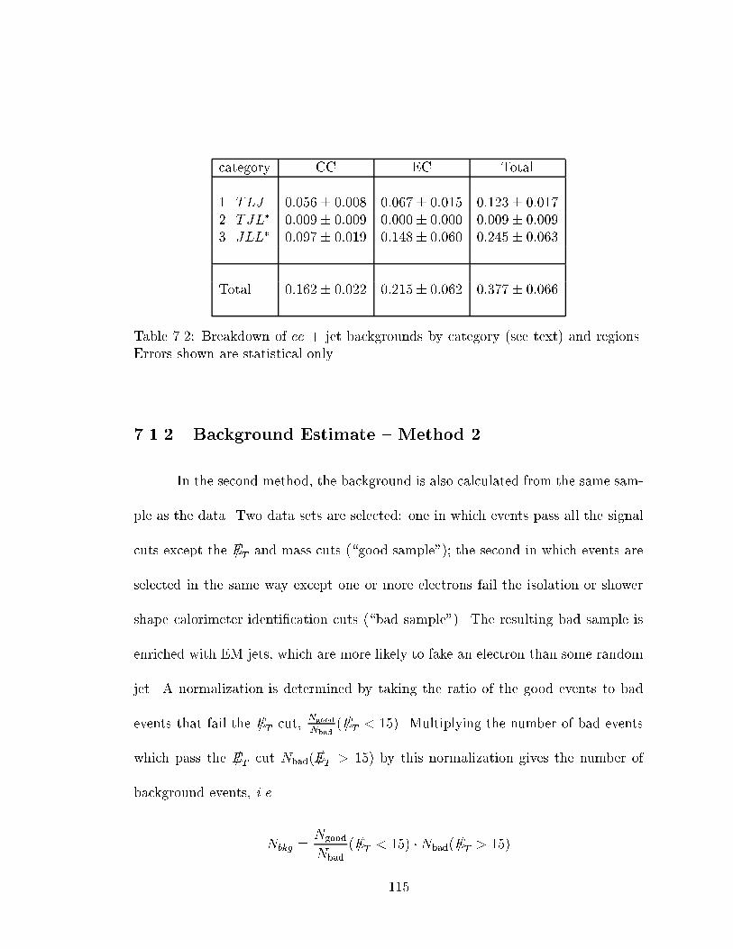
category CC EC Total

1. TLJ 0:056� 0:008 0:067� 0:015 0:123� 0:0172. TJL� 0:009� 0:009 0:000� 0:000 0:009� 0:0093. JLL� 0:097� 0:019 0:148� 0:060 0:245� 0:063

Total 0:162� 0:022 0:215� 0:062 0:377� 0:066

Table 7.2: Breakdown of ee + jet backgrounds by category (see text) and regions.Errors shown are statistical only.

7.1.2 Background Estimate { Method 2

In the second method, the background is also calculated from the same sam-

ple as the data. Two data sets are selected: one in which events pass all the signal

cuts except the E/T and mass cuts (\good sample"); the second in which events are

selected in the same way except one or more electrons fail the isolation or shower

shape calorimeter identi�cation cuts (\bad sample"). The resulting bad sample is

enriched with EM jets, which are more likely to fake an electron than some random

jet. A normalization is determined by taking the ratio of the good events to bad

events that fail the E/T cut,Ngood

Nbad(E/T < 15). Multiplying the number of bad events

which pass the E/T cut Nbad(E/T > 15) by this normalization gives the number of

background events, i.e.

Nbkg =Ngood

Nbad

(E/T < 15) �Nbad(E/T > 15)

115

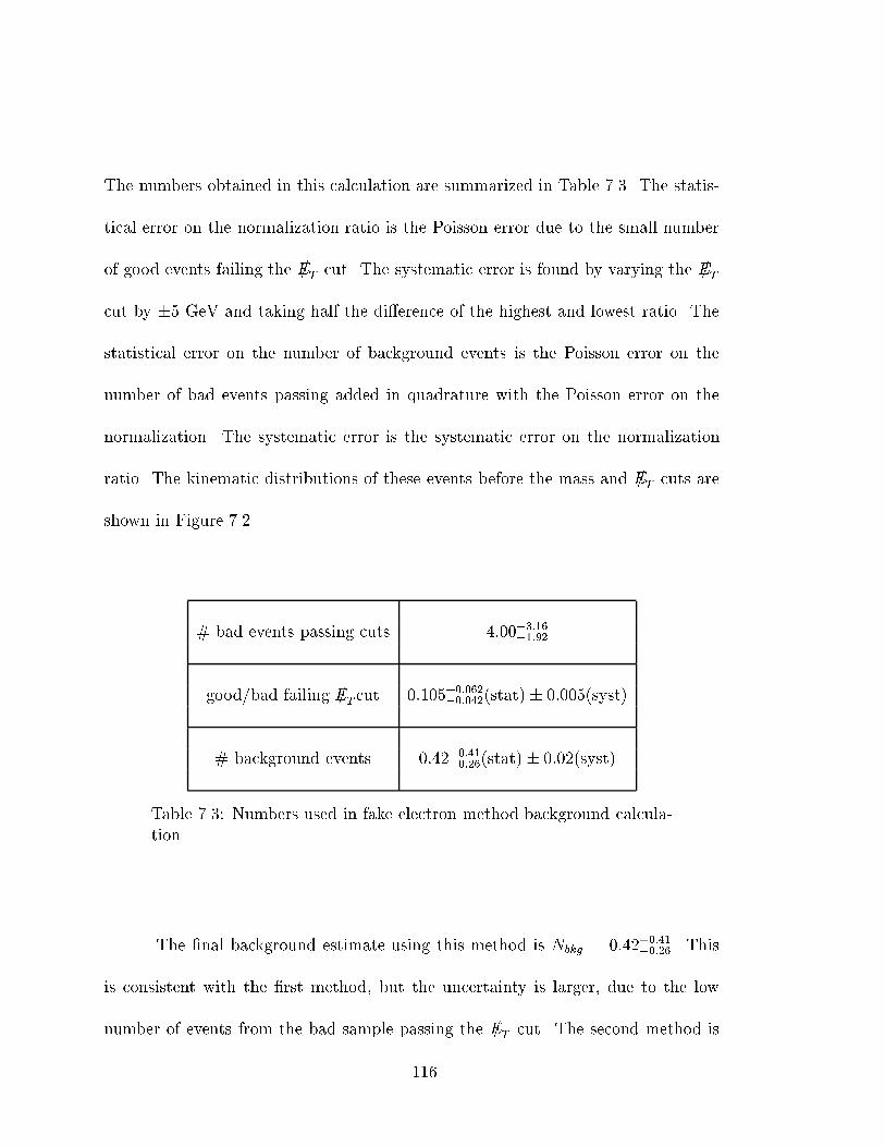
The numbers obtained in this calculation are summarized in Table 7.3. The statis-

tical error on the normalization ratio is the Poisson error due to the small number

of good events failing the E/T cut. The systematic error is found by varying the E/T

cut by �5 GeV and taking half the di�erence of the highest and lowest ratio. The

statistical error on the number of background events is the Poisson error on the

number of bad events passing added in quadrature with the Poisson error on the

normalization. The systematic error is the systematic error on the normalization

ratio. The kinematic distributions of these events before the mass and E/T cuts are

shown in Figure 7.2.

# bad events passing cuts 4:00+3:16�1:92

good/bad failing E/T cut 0:105+0:062�0:042(stat)� 0:005(syst)

# background events 0:42+0:41�0:26(stat)� 0:02(syst)

Table 7.3: Numbers used in fake electron method background calcula-tion.

The �nal background estimate using this method is Nbkg = 0:42+0:41�0:26. This

is consistent with the �rst method, but the uncertainty is larger, due to the low

number of events from the bad sample passing the E/T cut. The second method is

116

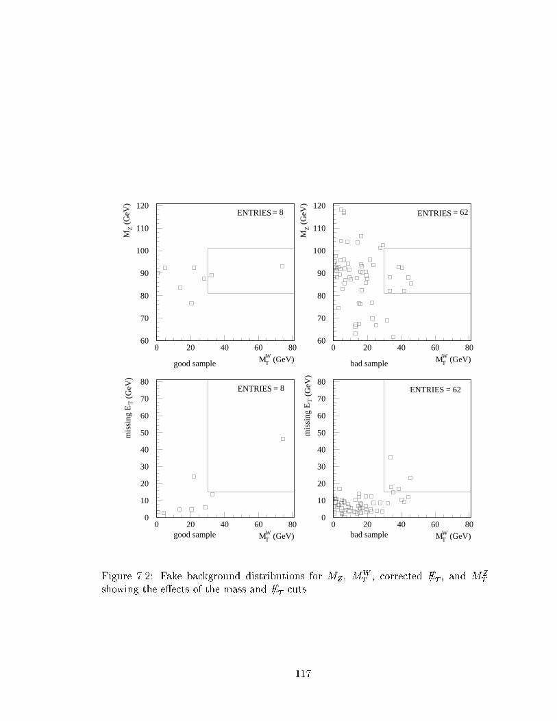
60

70

80

90

100

110

120

0 20 40 60 80

ENTRIES = 8

MTW (GeV)

MZ (

GeV

)

good sample

60

70

80

90

100

110

120

0 20 40 60 80

ENTRIES = 62

MTW (GeV)

MZ (

GeV

)

bad sample

0

10

20

30

40

50

60

70

80

0 20 40 60 80

ENTRIES = 8

MTW (GeV)good sample

0

10

20

30

40

50

60

70

80

0 20 40 60 80

ENTRIES = 62

MTW (GeV)bad sample

mis

sing

ET (

GeV

)

mis

sing

ET (

GeV

)

Figure 7.2: Fake background distributions for MZ , MWT , corrected E/T , and MZ

T

showing the e�ects of the mass and E/T cuts.

117

presented as a cross check to the �rst. For purposes of background subtraction, the

�rst method is preferred because of the smaller uncertainty.

7.2 Backgrounds for the WZ ! ��ee channel

As in the e�ee channel the backgrounds for this channel come from processes

in which a jet fakes the signature of an isolated muon or electron. The backgrounds

include ee+ jet where the jet produces an isolated muon and e�+ jet where the jet

fakes an electron. In both cases missing energy can result from the mismeasurement

of the jet or muon, and therefore a data-based technique must be used to estimate

the backgrounds.

7.2.1 ee + jet Background

Before proceeding it is necessary to calculate the probability of a jet produc-

ing an isolated muon. This probability was calculated from a sample of multijet

events by counting the number of events containing an isolated muon and dividing

by the total number of events in the sample. For a muon with pT > 15 GeV this

probability was found to be 1:5 � 10�5 [81]. In addition, the probability of a jet

faking a muon from a heavy quark (b=c) jet was found by requiring a muon ( iso-

lated on non-isolated ) in the opposite hemisphere from the isolated muon. This

gave a heavy quark enhanced fake rate of 2:5 � 10�4. A systematic uncertainty of

118

10% percent is assigned to both probabilities because of the small number of events

found with an isolated muon.

To calculate the ee + jet background, events with two electrons and a central

jet were selected from the Z ! ee sample. Each event was required to pass all cuts

except that the jet was only required to pass the muon �ducial and kinematic cuts.

The number of events (88) is then multiplied by the probability of the jet producing

an isolated muon. The number of events expected from this background is � 0:002.

A small fraction of the ee+jet events contain real heavy quark (b=c) jets. Assuming

that all of the jets in the fake sample are heavy quark jets and using the heavy quark

enhanced fake rate, we obtain an upper limit of Nbkg = 0:022 for this background.

However, to set a conservative limit, we take the smaller estimate and neglect this

background.

7.2.2 e� + jet Background

The second background (e� + jet) was calculated from the electroweak

group's 93-95 W ! e� data sample. Events in this sample required one EM object

above 10 GeV and E/T > 15 GeV. A background data sample was selected by re-

quiring events with an isolated muon, one or more jets and a tight or loose electron.

All event selection cuts were applied with the exception of the trigger, which was

replaced by the EM1 EIS TRKCC trigger. This trigger required one EM object and

missing energy at Level 2. A total of 60 events were selected.

119

The number of fake events is then found by multiplying by the ET -dependent

probability for a jet to fake an electron, accounting correctly for events which contain

more than one jet:

Nbkg = wtrig

NevtXj=1

0@NjetX

i=1

Pi(ET )

1A

where Nbkg is the estimated number of background events, Nevt is the number of

events in the background data sample, Njet is the number of jets in the event,

Pi(ET ) is the ET -dependent probability for jet i to fake an electron, and wtrig is

a factor to account for triggers (see below). Using this method, each jet in the

event is considered. The ET -dependent probability of the jet faking a tight or loose

electron is the same as in the WZ ! e�ee channel. The factor wtrig is the total

integrated luminosity of the 93-95 and 95-96 data sets divided by the integrated

luminosity of the 93-95 data set. This factor was necessary due to the lack of the

EM1 EIS TRKCC trigger in the 95-96 data set. Therefore, only the 93-95 data set

was used to estimate the background and a simple scaling of the background in

95-96 data set was assumed.

The total number of background events expected from e� + jet is 0:118 �

0:018(stat) � 0:035(syst). The systematic error is due to the 30% error on the

probability that a jet fakes an electron as mentioned previously.

The total number of background events from both sources of background is

0:118� 0:018(stat)� 0:035(syst).

120

Chapter 8

Results

8.1 Upper Limit on the WZ Cross Section

To set an upper limit on the cross section a Bayesian approach is used,

including convolution of the Poisson probability of observing a given number of

events with Gaussian probabilities for the expected signal and backgrounds. The

method is described in Reference [87], and brie y outlined below.

The expected number of events � is given by

� = � + �Xi

�iLiBri (8.1)

where� = expected number of background events in all channels� = cross section�i = e�ciency for channel i (i=1,2 for e�ee, ��ee)L = integrated luminosity for channel i

Bri = branching ratio for channel i

121

The factors multiplying the cross section are combined into one parameter �

� =Xi

�iLiBri (8.2)

so the expected number of events is given by

� = � + �� (8.3)

When calculating the error on � (��) only the error on the integrated lumi-

nosity is assumed to be correlated between channels. This is the most conservative

approach because other correlated errors exist between channels, including particle

identi�cation e�ciency errors and trigger e�ciency errors as will be discussed in the

next section.

The normalized probability that the \true" number of events is �, given the

observed number of events N is

P (�jN) =

�Ne��

N !NXk=0

�ke��

k!

(8.4)

where the physical region is given by � > 0, so that the normalization integral

includes only the region � > �.

The uncertainties in � and � are assumed to be uncorrelated, so that the

joint probability is the product of the individual probabilities. The probability

distribution for � is assumed to be described by a Gaussian distribution about its

122

nominal value �0

P (�) =e�

(���0)

2�2�Z 1

0e�

(���0)

2�2� d�

(8.5)

A similar probability distribution is assumed for �.

After integrating over � and � we obtain the probability distribution for �

P (�) =Z 1

0d�Z 1

0d�Z 1

�P (�jN)P (�)P (�)�

� � (�� �)

�

!d� (8.6)

where P (�) and P (�) are the probability densities for � and �.

Since each probability density is normalized separately, P (�) is also normal-

ized to unity. A con�dence limit is obtained by �nding the cross section where the

probability of the cross section being smaller is given by the con�dence level CL

Z �CL

0P (�)d� = CL (8.7)

Using this method, the 95% con�dence level limit on the cross section �(p�p!

WZ +X) was calculated to be 82:8 pb for the e�ee channel. The 95% con�dence

level limit on the WZ production cross section from the ��ee channel was found

to be 82.9 pb. Combining the e�ee channel and the ��ee channel, a combined 95%

con�dence level limit of 48.3 pb was obtained. The background, e�ciency, branching

ratio and integrated luminosity values used to set these limits are summarized in

Table 8.1. These limits are to be compared with a Standard Model cross section for

WZ production of 2.6 pb.

123

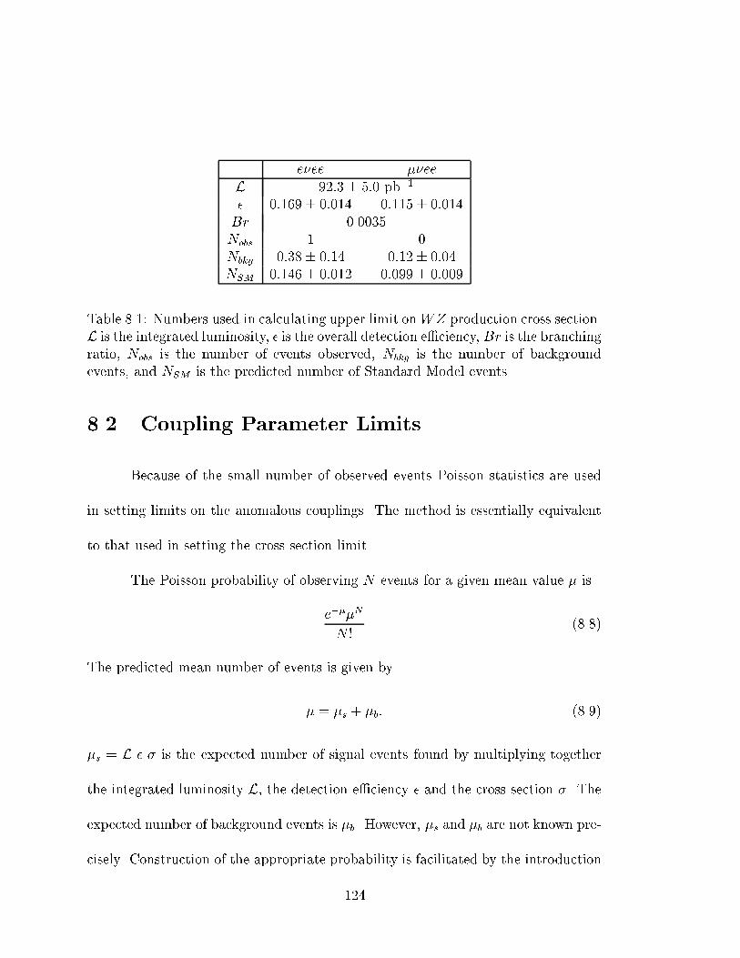
e�ee ��eeL 92:3� 5:0 pb�1

� 0:169� 0:014 0:115� 0:014Br 0.0035Nobs 1 0Nbkg 0:38� 0:14 0:12� 0:04NSM 0:146� 0:012 0:099� 0:009

Table 8.1: Numbers used in calculating upper limit onWZ production cross section.L is the integrated luminosity, � is the overall detection e�ciency, Br is the branchingratio, Nobs is the number of events observed, Nbkg is the number of backgroundevents, and NSM is the predicted number of Standard Model events.

8.2 Coupling Parameter Limits

Because of the small number of observed events Poisson statistics are used

in setting limits on the anomalous couplings. The method is essentially equivalent

to that used in setting the cross section limit.

The Poisson probability of observing N events for a given mean value � is

e���N

N !(8.8)

The predicted mean number of events is given by

� = �s + �b: (8.9)

�s = L � � is the expected number of signal events found by multiplying together

the integrated luminosity L, the detection e�ciency � and the cross section �. The

expected number of background events is �b. However, �s and �b are not known pre-

cisely. Construction of the appropriate probability is facilitated by the introduction

124

of a set of normalization parameters fxig. The probability density describing each

of the fxig is assumed to be described by a normalized Gaussian gi(xi; �i) centered

at unity:

gi(xi; �i) =e�

(xi�1)2

2�2iZ 1

0e�

(xi�1)2

2�2i dxi

(8.10)

where the unphysical region xi < 0 has been excluded. The mean number of ex-

pected events is

�x = xs L�� + xb �b (8.11)

where xs represents the signal prediction normalization and xb is the common back-

ground normalization. (By construction, the central value of all fxig is one.) Thus,

the probability for the ensemble of candidate events is given by

P =Zgs gb

e��x�NxN !

dxs dxb (8.12)

where N is the number of candidates, and �x is given by equation 8.11.

When combining results from more than one channel, it is important to

account for correlations in the uncertainties between the channels. For the case of the

e�ee and ��ee channels, there are both common and channel-speci�c normalization

uncertainties for both background and signal predictions. The mean number of e�ee

events becomes

�eee = xs;c xs;eee L��(WZ ! e�ee) + xb;c xb;eee �b;eee (8.13)

where xs;c represents the common signal prediction normalization, xs;eee is the

125

channel-speci�c signal prediction normalization, xb;c is the common background nor-

malization, and xb;eee is the channel-speci�c background normalization. The mean

number of ��ee events becomes

��ee = xs;c xs;�ee L��(WZ ! ��ee) + xb;c xb;�ee �b;�ee (8.14)

where the notation is similar to that used in Equation 8.13. The probability function

for both channels becomes

P =Zgs;c gb;c gs;eee gb;eee gs;�ee gb;�ee

� e��eee�Neee

N !

! e���ee�M�ee

M !

!

�dxs;c dxb;c dxs;eee dxb;eee dxs;�ee dxb;�ee (8.15)

where N is the number of observed e�ee events, M is the number of observed ��ee

events and �eee and ��ee are given by Equations 8.13 and 8.14 respectively.

The sources of common predicted signal normalization uncertainty are the

di-electron selection e�ciency error (0.98%), luminosity error (5.4%), theoretical

cross section error (6.2%) and trigger e�ciency error (2%). Added in quadrature

they give �c;s = 8:5%. The individual signal uncertainties come from identifying the

third lepton, 4.4% for the muon and 0.7% for the electron.

Both the e�ee and ��ee background estimates are based on the jet misiden-

ti�cation probabilities for electrons, which has a 30% normalization uncertainty.

126

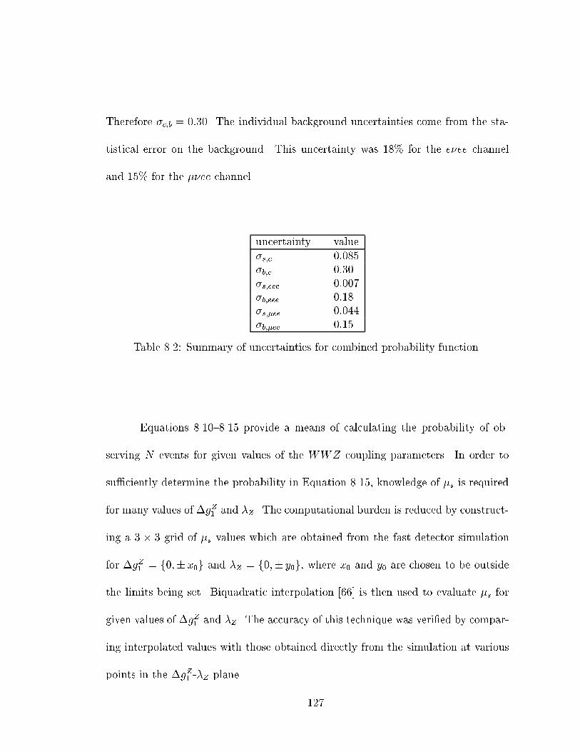
Therefore �c;b = 0:30. The individual background uncertainties come from the sta-

tistical error on the background. This uncertainty was 18% for the e�ee channel

and 15% for the ��ee channel.

uncertainty value�s;c 0:085�b;c 0:30�s;eee 0:007�b;eee 0:18�s;�ee 0:044�b;�ee 0:15

Table 8.2: Summary of uncertainties for combined probability function.

Equations 8.10{8.15 provide a means of calculating the probability of ob-

serving N events for given values of the WWZ coupling parameters. In order to

su�ciently determine the probability in Equation 8.15, knowledge of �s is required

for many values of �gZ1 and �Z. The computational burden is reduced by construct-

ing a 3 � 3 grid of �s values which are obtained from the fast detector simulation

for �gZ1 = f0;� x0g and �Z = f0;� y0g, where x0 and y0 are chosen to be outside

the limits being set. Biquadratic interpolation [66] is then used to evaluate �s for

given values of �gZ1 and �Z. The accuracy of this technique was veri�ed by compar-

ing interpolated values with those obtained directly from the simulation at various

points in the �gZ1 -�Z plane.

127

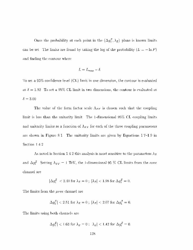
Once the probability at each point in the (�gZ1 ; �Z){plane is known limits

can be set. The limits are found by taking the log of the probability (L = � lnP )

and �nding the contour where

L = Lmax � �:

To set a 95% con�dence level (CL) limit in one dimension, the contour is evaluated

at � = 1:92. To set a 95% CL limit in two dimensions, the contour is evaluated at

� = 3:00.

The value of the form factor scale �FF is chosen such that the coupling

limit is less than the unitarity limit. The 1-dimensional 95% CL coupling limits

and unitarity limits as a function of �FF for each of the three coupling parameters

are shown in Figure 8.1. The unitarity limits are given by Equations 1.7{1.9 in

Section 1.4.2.

As noted is Section 1.4.2 this analysis is most sensitive to the parameters �Z

and �gZ1 . Setting �FF = 1 TeV, the 1-dimensional 95 % CL limits from the e�ee

channel are

j�gZ1 j < 2:40 for �Z = 0 ; j�Zj < 1:98 for �gZ1 = 0:

The limits from the ��ee channel are

j�gZ1 j < 2:51 for �Z = 0 ; j�Zj < 2:07 for �gZ1 = 0:

The limits using both channels are

j�gZ1 j < 1:63 for �Z = 0 ; j �Zj < 1:42 for �gZ1 = 0:

128

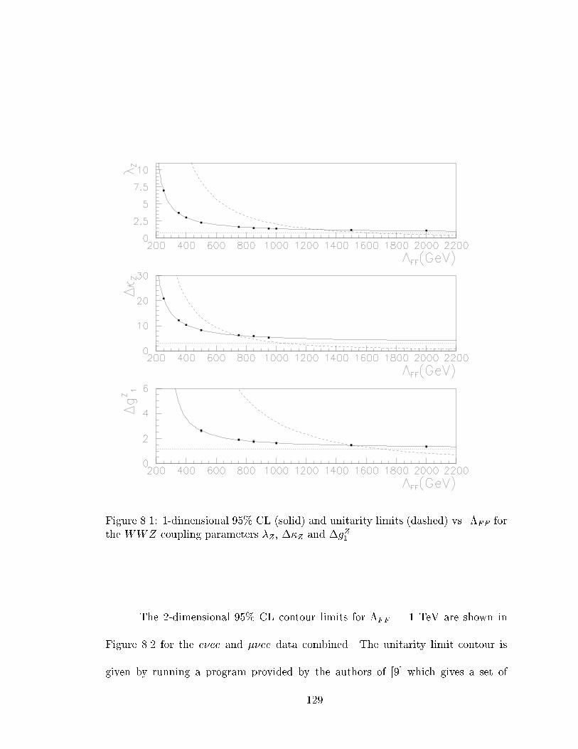
Figure 8.1: 1-dimensional 95% CL (solid) and unitarity limits (dashed) vs. �FF forthe WWZ coupling parameters �Z , ��Z and �gZ1 .

The 2-dimensional 95% CL contour limits for �FF = 1 TeV are shown in

Figure 8.2 for the e�ee and ��ee data combined. The unitarity limit contour is

given by running a program provided by the authors of [9] which gives a set of

129

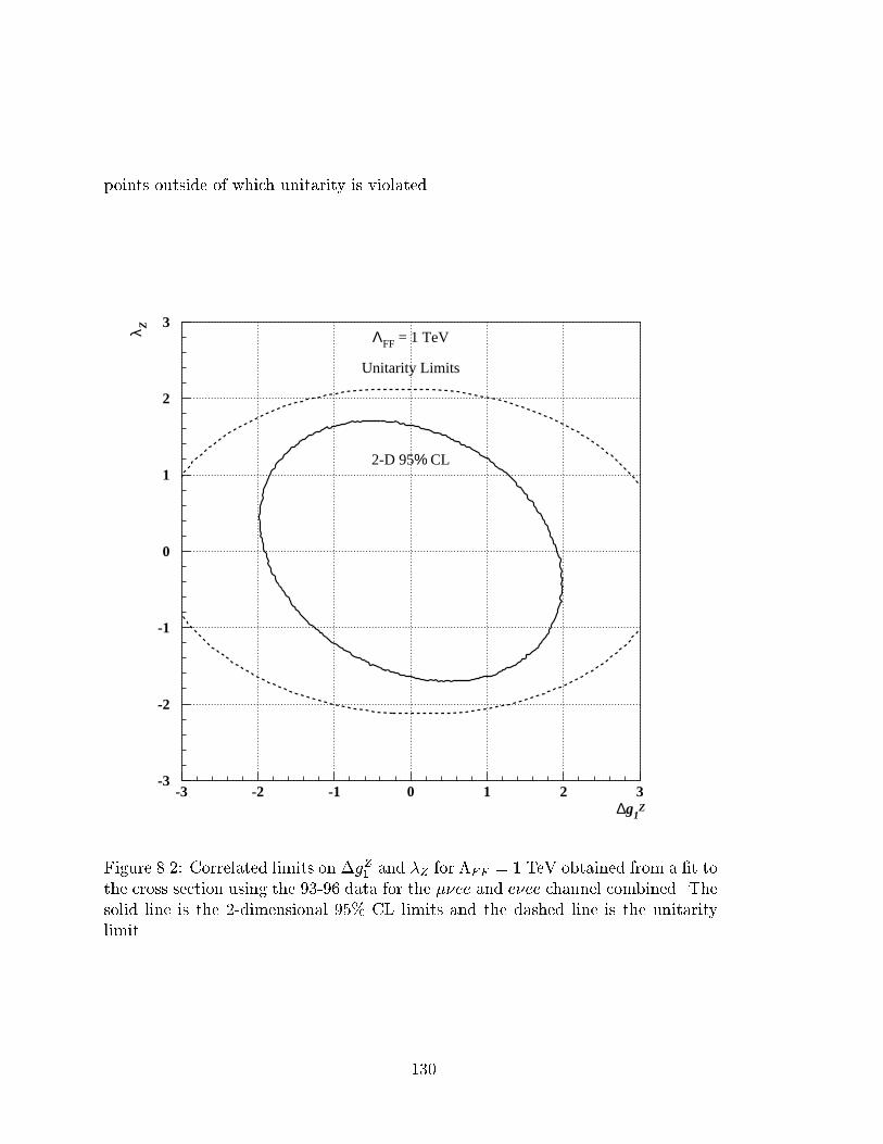
points outside of which unitarity is violated.

-3

-2

-1

0

1

2

3

-3 -2 -1 0 1 2 3∆g1

Z

λ Z

Unitarity Limits

ΛFF = 1 TeV

2-D 95% CL

Figure 8.2: Correlated limits on �gZ1 and �Z for �FF = 1 TeV obtained from a �t tothe cross section using the 93-96 data for the ��ee and e�ee channel combined. Thesolid line is the 2-dimensional 95% CL limits and the dashed line is the unitaritylimit.

130

Chapter 9

Conclusions

9.1 Summary

A search for WZ production in the e�ee and ��ee channel was performed

using 92:3 � 5:0 pb�1 of data recorded by the D� detector in p�p collisions atps

= 1.8 TeV during the 1993-1996 data taking runs. One event is observed with an

expected Standard Model signal of 0:245� 0:002 (stat) � 0:015 (syst) events and an

expected background of 0:498 � 0:072 (stat) � 0:125 (syst) events. This does not

represent a signi�cant excess of WZ events. The 95% upper con�dence limit on the

WZ production cross section is found to be 48:3 pb. A �t to the expected number

of events as function of the coupling parameters is performed and limits are set.

Assuming only one parameter varies at a time the 95% CL limits are j�gZ1 j < 1:63

and j�Zj < 1:42 for a form factor scale of �FF = 1 TeV. Although the limits are

131

looser than those previously measured, they are independent of the WW vertex

coupling. Previous results have relied on making assumptions about the relation

between the WW and WWZ couplings.

9.2 Future Prospects

With an expected 2 fb�1 of data to be delivered in the next Tevatron collider

run and an upgraded D� detector, it will be possible to observe a signi�cant WZ

production signal in the l�ll �nal state. This will enable the direct measurement of

the cross section instead of placing upper limits and will result in tighter limits on

the WWZ coupling parameters.

132

Bibliography

[1] S. Abachi, et al. (D� Collaboration), \Observation of the Top Quark", Phys.

Rev. Lett. 74, 2632 (1995).

[2] F. Abe, et al. (CDF Collaboration), \Observation of the Top Quark in p�p

Collisions", Phys. Rev. Lett. 74, 2626 (1995).

[3] S. Weinberg, Phys. Rev. Lett. 19, 1264 (1967).

[4] A. Salam in Elementary Particle Theory, ed. N. Svarthom, et al. Stockholm

(1968);

M.E. Peskin , D.V. Schroeder An Introduction to Quantum Field Theory.

Addison-Wesley (1995);

S. Weinberg The Quantum Theory of Fields. Cambrisge, UK: Cambridge Univ.

Press (1995).

[5] F. Halzen and A. Martin, Quarks and Leptons, John Wiley & Sons, Inc. (1994).

133

[6] UA1 Collaboration, \Experimental Observation of Isolated Large Transverse

Energy Electrons with Associated Missing Energy atps = 540 GeV." Phys.

Lett. B122, 103 (1983);

UA2 Collaboration, \Observation of Single Isolated Electron with High Trans-

verse Momentum in Events with Missing Transverse Energy at the CERN p�p

Collider." Phys. Lett. B122, 476 (1983).

[7] UA1 Collaboration, \Experimental Observation of Lepton Pairs of Invariant

Mass around 95 GeV/c2." Phys. Lett. B126, 398 (1983);

UA2 Collaboration, \Evidence for Z0 ! e+e� at the CERN p�p Collider." Phys.

Lett. B129, 130 (1983).

[8] T. Sjostrand, \PYTHIA 5.7 and JETSET 7.4: Physics and Manual" Comput.

Phys. Commun 82, 74, (1994).

[9] K. Hagiwara, J. Woodside, and D. Zeppenfeld, Phys. Rev. D41, 2113 (1990).

[10] A. Martin, W. Stirling, and R. Roberts, \New Information on Parton Distri-

butionns." Phys. Rev. D47, 867 (1993);

\Parton Distributions Updated." Phys. Lett. B306, 145 (1993).

[11] V. Barger and R. Philips, Collider Physics. Frontiers In Physics Lecture Note

Series, Addison-Wesley (1987).

[12] J. Papavassiliou, K. Philippides, Phys.Rev. D48, 4255 (1993).

134

[13] J. Koidaira, et al. in INS Workshop Phys. e+e�, e� and Collis. at Linear

Accel.. Tokyo, Japan, Dec. 20{22, 1994, ed. Z. Hioki, T. Ishii, R. Najima. Tokyo

Univ., Inst. Nucl. Study (1995).

[14] D. Chang , W.-Y. Keung, Nucl. Phys. B355, 295 (1991).

[15] I.B. Khriplovich , M.E. Pospelov, Nucl. Phys. B420, 505 (1994).

[16] G. Couture, et al., Phys. Rev. D36, 859 (1987).

[17] X.-G. He, B.H.J. McKellar, Phys. Rev. D42, 3221 (1990);

Phys. Rev. D50 4719 (1994).

[18] G. Couture, J.N. Ng, Z. Phys C35, 65 (1987).

[19] E.N. Argyres, et al., Phys. Rev. B383, 63 (1996).

[20] T. Kadoyoshi, N. Oshimo, Phys. Rev. D55, 1481 (1997).

[21] T. Appelquist, G.-H. Wu, Phys. Rev. D48, 3235 (1993);

Phys. Rev. D51, 240.

[22] C.P. Burgess, A. Pilaftsis, Phys. Rev. B333, 427.

[23] J. Ellison and J. Wudka, \Study of Trilinear Gauge Boson Couplings at

the Tevatron Collider", to be published in Ann. Rev. Nucl. Part. Sci.,

UCR/D�/9801, hep-ph/9804322 (1998).

135

[24] K. Hagiwara, R.D. Peccei, D. Zeppenfeld amd K. Hikasa, Nucl. Phys. B282,

253 (1987).

[25] K. Hagiwara, S. Ishihara, R. Szalapski and D. Zeppenfeld, Phys. Rev. D48,

2182 (1993); Phys. Lett. B283, 353 (1993).

[26] U. Baur and D. Zeppenfeld, Phys. Lett. B201, 383 (1988).

[27] H. Aihara et al., Preprint Fermilab-Pub-95/031 (1995).

[28] J. Alitti et al. (UA2 Collaboration), Phys. Lett. B277, 195 (1992).

[29] F. Abe et al. (CDF Collaboration), Phys. Rev. Lett. 74, 1936 (1995);

Phys. Rev. Lett. 75, 1017 (1995).

[30] S. Abachi et al. (D� Collaboration), Phys. Rev. Lett. 78, 3634 (1997).

[31] F. Abe et al. (CDF Collaboration), Phys. Rev. Lett. 74, 1936 (1995).

[32] B. Abbot et al. (D� Collaboration), Phys. Rev. Lett. 79, 1441 (1997).

[33] F. Abe et al. (CDF Collaboration), Phys. Rev. Lett. 78, 4537 (1997).

[34] B. Abbot et al. (D� Collaboration), to be published in Phys. Rev. D, Rapid

Communications (1998), FERMILAB PUB 98-076-E, hep-ex/9803004

[35] J. Ellison, \Measurement of the W Boson Mass and Trilinear Gauge Boson

Couplings at the Tevatron" to be published in Proceedings of the XXXIIId

136

Rencontres de Moriond, Electroweak Interactions and Uni�ed Theories, Les

Arcs, Savoie, France, March 14-21 1998.

[36] J-M. Jousset, \A combination of Preliminary Measurements of Triple Gauge

Boson Coupling Parameters by the LEP and D� Experiments" to be published

in Proceedings of the XXXIIId Rencontres de Moriond, Electroweak Interactions

and Uni�ed Theories, Les Arcs, Savoie, France, March 14-21 1998.

[37] L. M. Lederman, Scienti�c American 264(3) 48 (Mar. 1991);

H. T. Edwards, Ann. Rev. Nucl. Part. Sci. 35, 605 (1985;).

F. T. Cole et al., \Design Report Tevatron 1 Project," FNAL Internal Note

(1984;), unpublished.

F. T. Cole et al., \A Report of the Design of the Fermi National Laboratory

Superconducting Accelerator," FNAL Internal Note (1979.), unpublished.

[38] W. J. Thompson, \Introduction to Colliding Beams at Fermilab," D� Internal

Note 2367 (1994), unpublished.

[39] D. M�ohl et al., Phys. Rep. C58, 73 (1980).

[40] S. Abachi et al., Nucl. Instr. Meth. A338, 185 (1994).

[41] S. Snyder, \The D� Detector," D� Internal Note 2500 (1995), unpublished.

137

[42] F. Sauli, Principles of Operation of Multiwire Proportional and

Drift Chambers in T. Ferbel, editor, Experimental Techniques in High Energy

Physics. Addison-Wesley (1987).

[43] R. C. Fernow, Introduction to Experimental Particle Physics. Cambridge Uni-

versity Press (1986).

[44] K. Kleinknecht, Detectors for Particle Radiation. Cambridge University Press

(1987).

[45] A. R. Clark et al., Nucl. Instr. Meth. A261, 420 (1987).

[46] A. R. Clark et al., Nucl. Instr. Meth. A279, 243 (1989).

[47] A. R. Clark et al., Nucl. Instr. Meth. A315, 193 (1992).

[48] J. F. Det�uf et al., Nucl. Instr. Meth. A265, 157 (1988).

[49] J. F. Det�uf et al., Nucl. Instr. Meth. A279, 310 (1989).

[50] D. Buchholz et al., Nucl. Instr. Meth. A257, 556 (1987).

[51] T. Behnke, The Central Drift Chamber for the D� Detector: Design, Construc-

tion, and Test. Ph.D. thesis, State University of New York at Stony Broook,

Stony Brook, New York, 1989 (unpublished).

138

[52] D. Pizzuto, D� Central Tracking Performance Studies. Ph.D. thesis, State

University of New York at Stony Broook, Stony Brook, New York, 1991 (un-

published).

[53] S. Rajagopalan, The dE=dx Capabilities of the D� Tracking System. Ph.D.

thesis, Northwestern University, Evanston, Illinois, 1992 (unpublished).

[54] J. W. Bantly, The D� Forward Drift Chamber Performance and Physics Capa-

bility in the 1990 FNAL Testbeam Run. Ph.D. thesis, Northwestern University,

Evanston, Illinois, 1992 (unpublished).

[55] C. Fabjan, Calorimetry in High-Energy Physics in T. Ferbel, editor, Ex-

perimental Techniques in High Energy Physics. Addison-Wesley (1987).

[56] U. Amaldi, Fluctuations in Calorimetry Measurements in T. Ferbel, edi-

tor, Experimental Techniques in High Energy Physics. Addison-Wesley (1987).

[57] C. Brown, et al., Nucl. Instr. Meth. A279, (1989).

[58] J. Bantly, et al., \Improvement to the D� Luminosity Constant." D� Internal

Note 2544 (1995.), unpublished.

[59] J. Butler, \Main Ring Deadtime," D� Internal Note 1682 (1993), unpublished.

[60] M. Abolins, et al., \The Fast Trigger for the D� Experiment." Nuclear Instru-

ments and Methods A289, 543, (1990).

139

[61] J. Bantly, et al., \The D� Level 1.5 Calorimeter Trigger." D� Internal Note

2147 (1994), unpublished.

[62] Fatyga, M. \Tuning Electron Id Parameters for the Level 2 Trigger Using Test-

beam Data." D� Internal Note 1768 (1994), unpublished.

[63] G. Manning, \D� Software Documentation." D� Internal Document

July 10,1995.

(URL: http://www-d0.fnal.gov/software/offline document.ps)

[64] N. Graf, D� Internal Note (in preparation).

[65] T. Yasuda, \A Study of CDC z Measurement Using Collider Muon Tracks,"

D� Internal Note 2782 (1995), unpublished.

[66] S. Glenn, A Search for Self Interactions of Neutral Electroweak Gauge Bosons.

Ph.D. thesis, University of California at Davis, Davis, California, 1996 (unpub-

lished).

[67] S. Youssef, \A Family of Cluster Algorithms," D� Internal Note 375 (1986),

unpublished.

[68] S. Youssef, \Clustering with Local Equivalence Relations," D� Internal Note

541 (1987), unpublished.

140

[69] N. Graf, \Simulation of the Level 1 CC Edge E�ect," D� Internal Note 1339

(1992), unpublished.

[70] N. Graf, \Improvements to the Calorimeter Electron Position Algorithm," D�

Internal Note 1352 (1992), unpublished.

[71] A. Goldschmidt and S. Glenn, \Corrections to Biases in Cluster-Track Match-

ing," D� Internal Note 2419 (1995), unpublished.

[72] R. Raja et al., \Reconstruction and Analysis: Trcaking Packages, Calorimeter

Packages," D� Internal Note 1006 (1990), unpublished.

[73] R. Raja, \H-matrix Analysis for top! lepton + jets," D� Internal Note 1192

(1992), unpublished.

[74] M. Narain, Electron Identification in the D� Detector, in Proceedings

of the American Physical Society Division of Particles and Fields Conference,

Fermilab, Batavia, Illinois (1992).

[75] R. Kehoe, Search for the Top Quark in Dielectron Final States at sqrts = 1:8

TeV and Measurement of the Response of the D� U/LAr Calorimeter to Jets.

Ph.D. thesis, University of Notre Dame, Notre Dame, Indiana, 1997 (Unpub-

lished).

141

[76] S. Glenn, A Search for Self Interactions of Neutral Electroweak Gauge Bosons.

Ph.D. thesis, University of California at Davis, Davis, California, 1996 (Unpub-

lished).

[77] T. Yasuda, et al., \Muon Chamber Alignment" D� Internal Note 2279 (1994.),

unpublished.

[78] D. Casey, T. Jo�e-Minor and J. Tarazi, \QCD/WZ Ntuple", D� Internal Note

3124 (191996), unpublished.

[79] F. Carminati,et. al., GEANT Users Guide, CERN Library Program Entry

W5013 (1993).

[80] D. Norman, \Improved Low ET Electron Identi�cation using Lower Dimen-

sional H-Matrices and Fisher Variables." D� Internal Note 2453 (1995), un-

published.

[81] P. Bloom. Investigation of the Trilinear Vector Boson Couplings Through W

Boson Pair Production in the Dilepton Decay Channels Ph.D. thesis, University

of California at Davis, Davis, California, 1998 (Unpublished).

[82] B. Abbot et. al. (D� Collaboration), to be published in Phys. Rev. D, Rapid

Communications (1998), FERMILAB PUB 98-076-E, hep-ex/9803004

[83] S. Glenn, \A Parametric Detector Simulation for Dibosons." D� Internal Note

2846 (1996), unpublished.

142

[84] D. Wood, et. al. , D� Internal Note 2140 (19.), unpublished.

[85] S. Glenn. \A Study of Electron and Photon Fakes", D� Internal Note 2937

(1996), unpublished.

[86] O. Helene, Nucl. Instr. and Methods 212 (1983) 319; Nucl. Instr. and Methods

228 (1984) 120.

[87] R. Partridge, D� Internal Note 1806 (1993.), unpublished.

143

Appendix A

Candidate Event Properties

The properties of the e�ee candidate event are listed below. Table A.1 lists

the properties of the electron candidates. Table A.2 lists the kinematic properties

of the event.

144

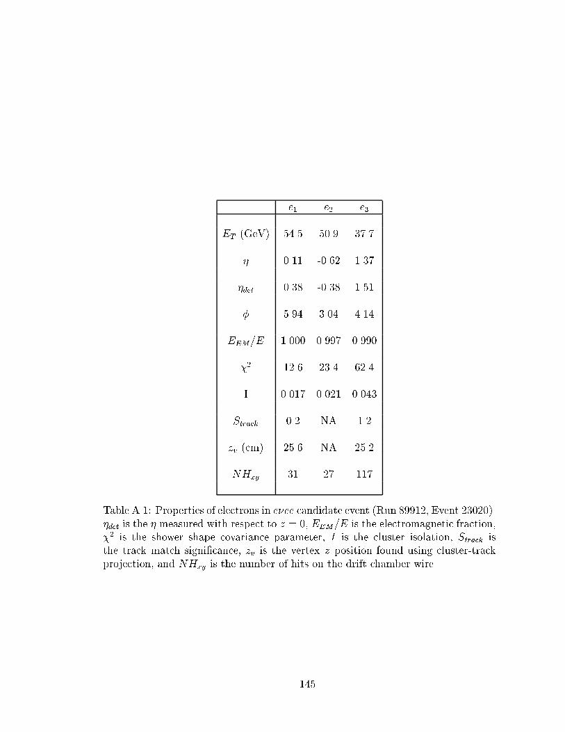
e1 e2 e3

ET (GeV) 54.5 50.9 37.7

� 0.11 -0.62 1.37

�det 0.38 -0.38 1.51

� 5.94 3.04 4.14

EEM=E 1.000 0.997 0.990

�2 12.6 23.4 62.4

I 0.017 0.021 0.043

Strack 0.2 NA 1.2

zv (cm) 25.6 NA 25.2

NHxy 31 27 117

Table A.1: Properties of electrons in e�ee candidate event (Run 89912, Event 23020).�det is the � measured with respect to z = 0, EEM=E is the electromagnetic fraction,�2 is the shower shape covariance parameter, I is the cluster isolation, Strack isthe track match signi�cance, zv is the vertex z position found using cluster-trackprojection, and NHxy is the number of hits on the drift chamber wire.

145

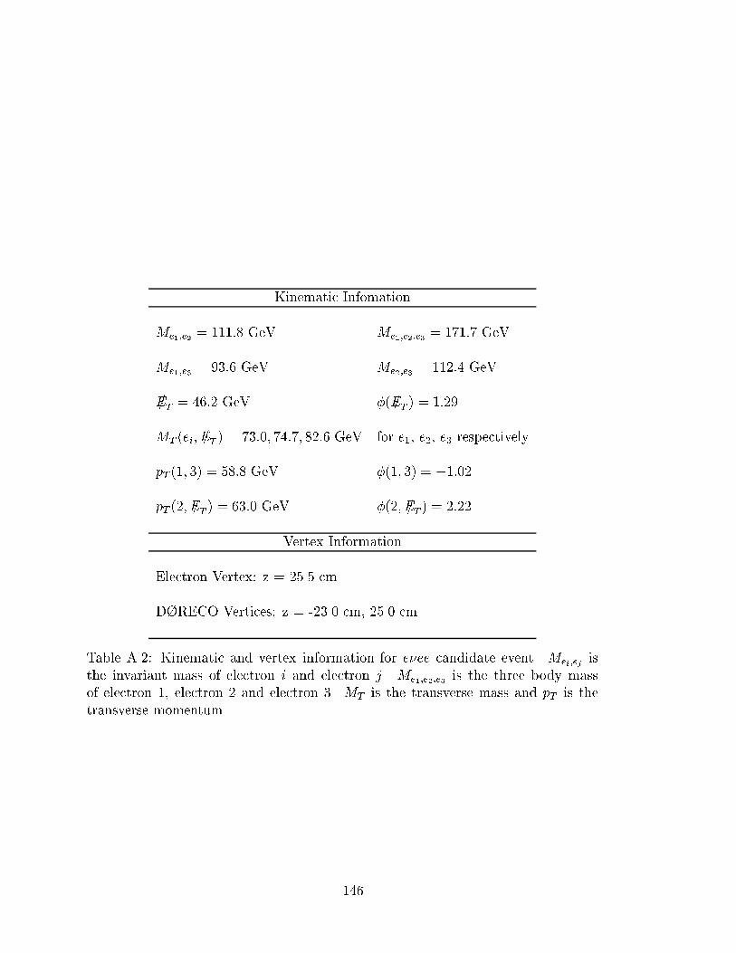
Kinematic Infomation

Me1;e2 = 111:8 GeV Me1;e2;e3 = 171:7 GeV

Me1;e3 = 93:6 GeV Me2;e3 = 112:4 GeV

E/T = 46:2 GeV �(E/T ) = 1:29

MT (ei; E/T ) = 73:0; 74:7; 82:6 GeV for e1, e2, e3 respectively

pT (1; 3) = 58:8 GeV �(1; 3) = �1:02

pT (2; E/T ) = 63:0 GeV �(2; E/T ) = 2:22

Vertex Information

Electron Vertex: z = 25.5 cm

D�RECO Vertices: z = -23.0 cm, 25.0 cm

Table A.2: Kinematic and vertex information for e�ee candidate event. Mei;ej isthe invariant mass of electron i and electron j. Me1;e2;e3 is the three body massof electron 1, electron 2 and electron 3. MT is the transverse mass and pT is thetransverse momentum.

146