Embed Size (px)
Citation preview
LU Decomposition
1

Introduction• Another way of solving a system of equations is by using a
factorization technique for matrices called LU decomposition. • This factorization is involves two matrices, one lower triangular
matrix and one upper triangular matrix.• LU factorization methods separate the time-consuming
elimination of the matrix [A] from the manipulations of the right-hand-side [b].
• Once [A] has been factored (or decomposed), multiple right-hand-side vectors can be evaluated in an efficient manner.
2
LU Decomposition
and
Where,
3
mm
m
m
u
uu
uuu
U
00
0 222
11211
mmmm lll
ll
l
L
21
2221
11
0
00
LUA
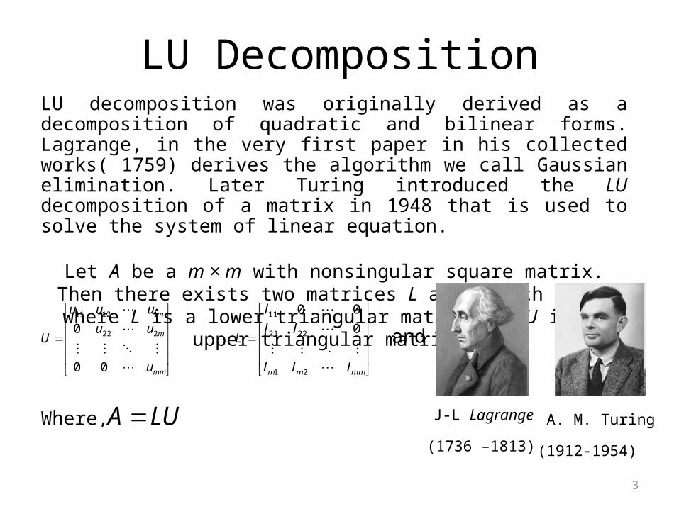
LU decomposition was originally derived as a decomposition of quadratic and bilinear forms. Lagrange, in the very first paper in his collected works( 1759) derives the algorithm we call Gaussian elimination. Later Turing introduced the LU decomposition of a matrix in 1948 that is used to solve the system of linear equation.
Let A be a m × m with nonsingular square matrix. Then there exists two matrices L and U such that, where L is a lower
triangular matrix and U is an upper triangular matrix.
J-L Lagrange
(1736 –1813) A. M. Turing
(1912-1954)
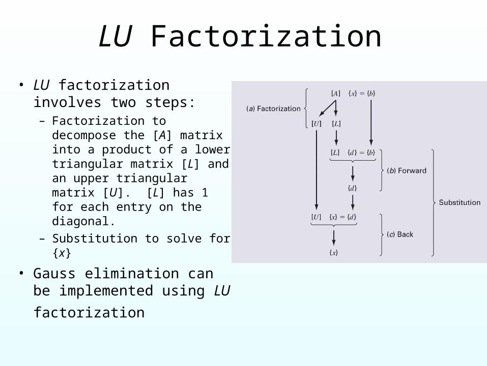
LU Factorization• LU factorization involves two
steps:– Factorization to decompose the
[A] matrix into a product of a lower triangular matrix [L] and an upper triangular matrix [U]. [L] has 1 for each entry on the diagonal.
– Substitution to solve for {x}
• Gauss elimination can be implemented using LU
factorization
LU Decomposition
5
LU Decomposition is another method to solve a set of simultaneous linear equations
Which is better, Gauss Elimination or LU Decomposition?
To answer this, a closer look at LU decomposition is needed.
MethodFor most non-singular matrix [A] that one could conduct Naïve Gauss Elimination forward elimination steps, one can always write it as
[A] = [L][U]
where
[L] = lower triangular matrix
[U] = upper triangular matrix
LU Decomposition
6
How does LU Decomposition work?
7
LU Decomposition
8
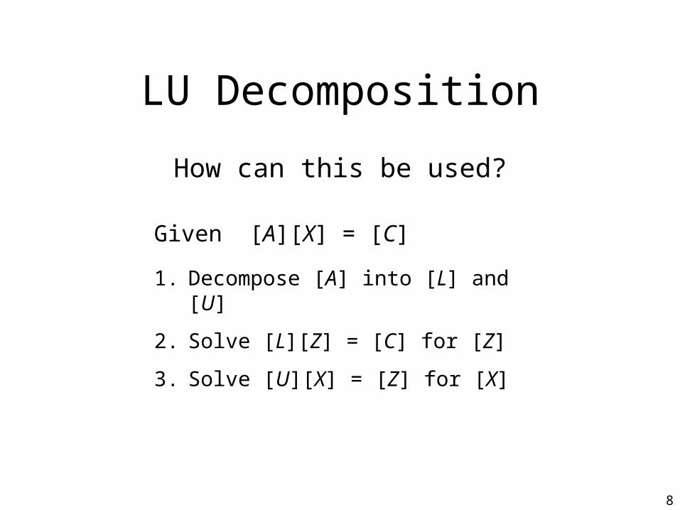
How can this be used?
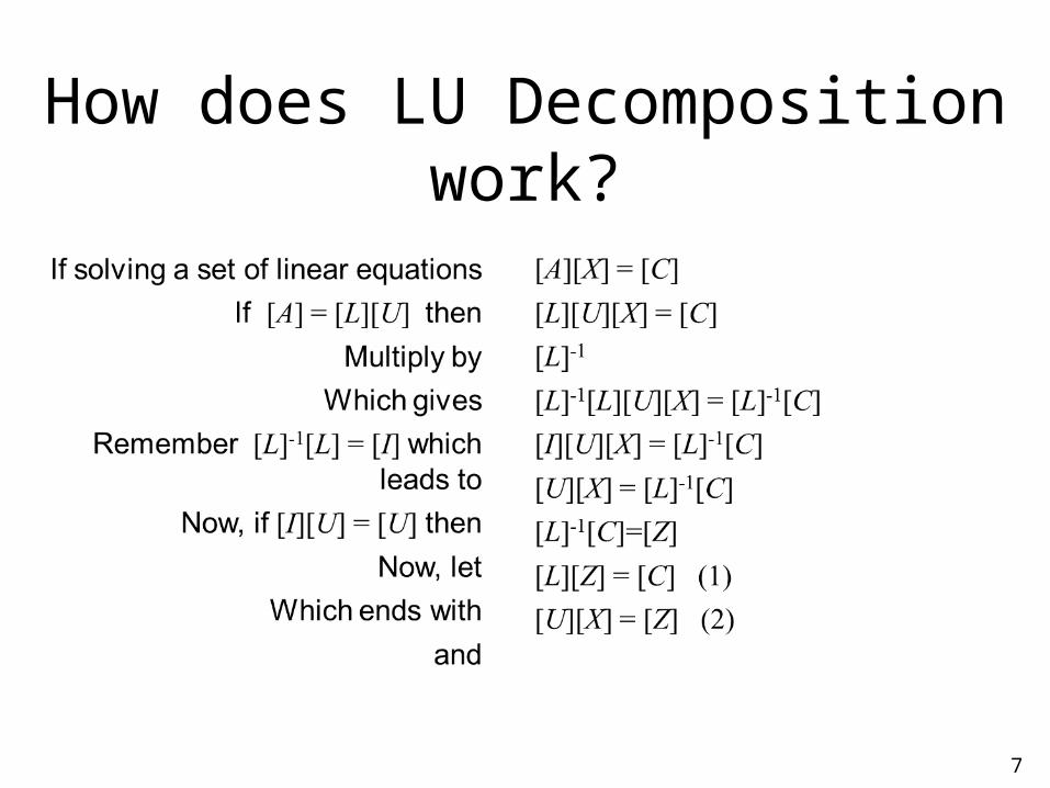
Given [A][X] = [C]
1. Decompose [A] into [L] and [U]
2. Solve [L][Z] = [C] for [Z]
3. Solve [U][X] = [Z] for [X]
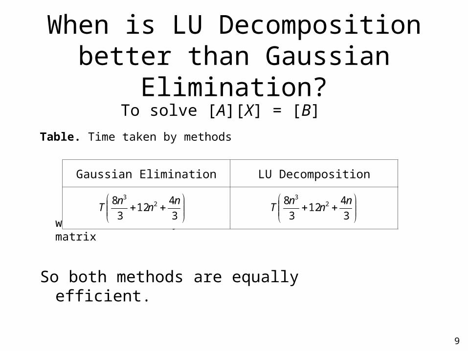
When is LU Decomposition better than Gaussian Elimination?
To solve [A][X] = [B]
Table. Time taken by methods
where T = clock cycle time and n = size of the matrix
So both methods are equally efficient.
9
Gaussian Elimination LU Decomposition
3
412
3
8 23 n
nn
T
3
412
3
8 23 n
nn
T
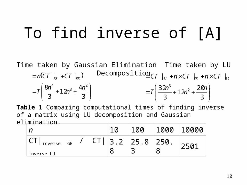
To find inverse of [A]
10
Time taken by Gaussian Elimination Time taken by LU Decomposition
3
412
3
8
||2
34 n
nn
T
CTCTn BSFE
3
2012
3
32
|||
23 n
nn
T
CTnCTnCT BSFSLU
n 10 100 1000 10000
CT|inverse GE / CT|inverse LU 3.28 25.83 250.8 2501
Table 1 Comparing computational times of finding inverse of a matrix using LU decomposition and Gaussian elimination.
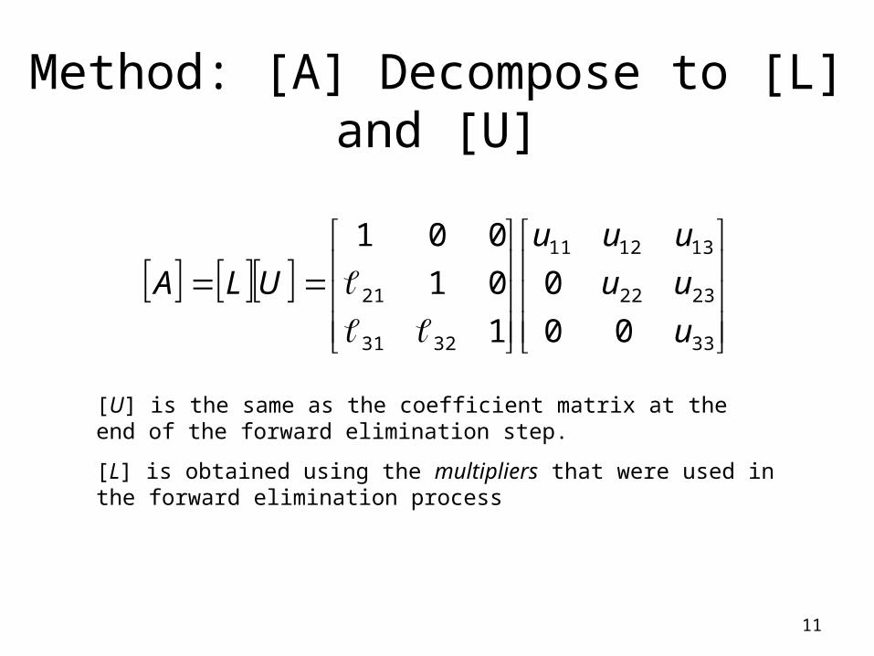
Method: [A] Decompose to [L] and [U]
11
33
2322
131211
3231
21
00
0
1
01
001
u
uu
uuu
ULA
[U] is the same as the coefficient matrix at the end of the forward elimination step.
[L] is obtained using the multipliers that were used in the forward elimination process

Finding the [U] matrix
12
Using the Forward Elimination Procedure of Gauss Elimination
112144
1864
1525
112144
56.18.40
1525
56.212;56.225
64
RowRow
76.48.160
56.18.40
1525
76.513;76.525
144
RowRow
Step 1:
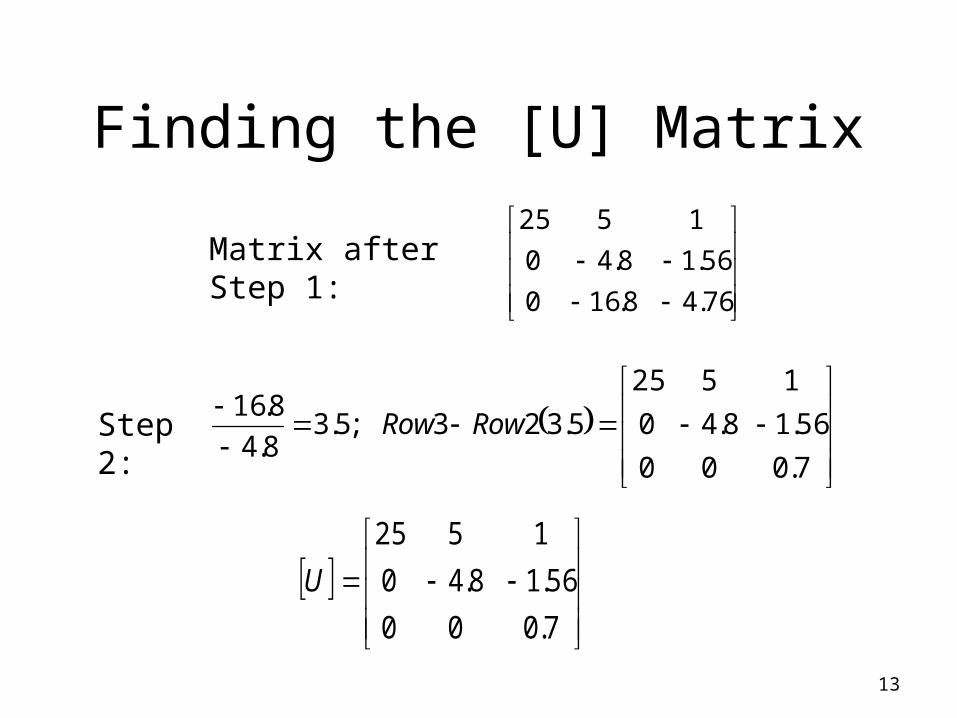
Finding the [U] Matrix
13
Step 2:
76.48.160
56.18.40
1525
7.000
56.18.40
1525
5.323;5.38.4
8.16
RowRow
7.000
56.18.40
1525
U
Matrix after Step 1:

Finding the [L] matrix
14
Using the multipliers used during the Forward Elimination Procedure
1
01
001
3231
21
56.225
64
11
2121
a
a
76.525
144
11
3131
a
a
From the first step of forward elimination
112144
1864
1525

Finding the [L] Matrix
15
15.376.5
0156.2
001
L
From the second step of forward elimination
76.48.160
56.18.40
15255.3
8.4
8.16
22
3232
a
a
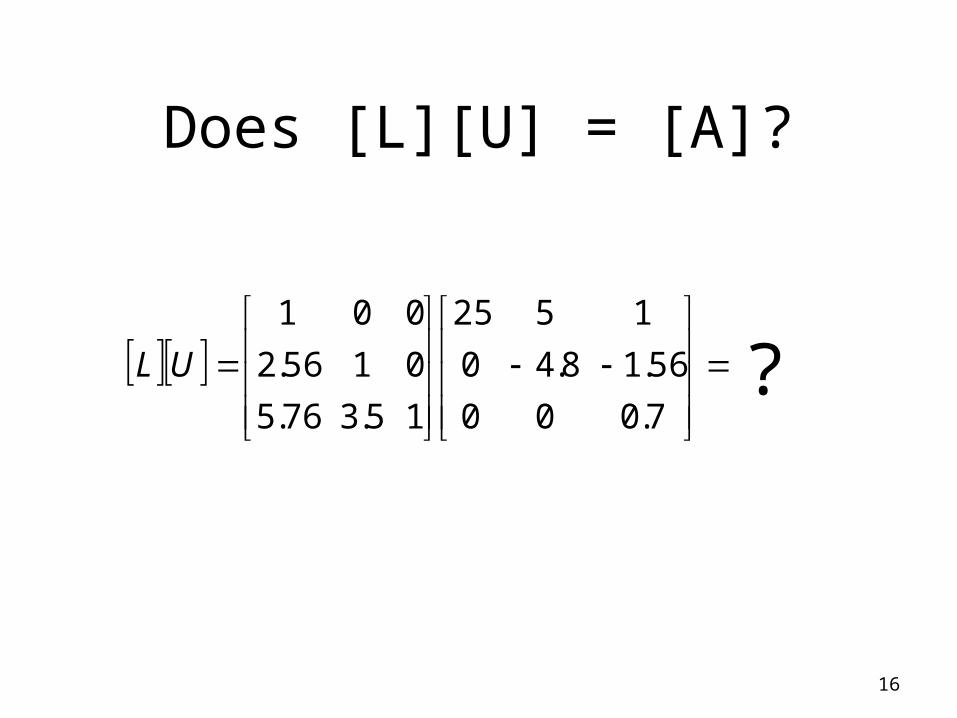
Does [L][U] = [A]?
16
7.000
56.18.40
1525
15.376.5
0156.2
001
UL ?
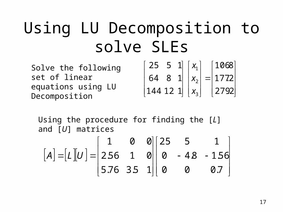
Using LU Decomposition to solve SLEs
17
Solve the following set of linear equations using LU Decomposition
2279
2177
8106
112144
1864
1525
3
2
1
.
.
.
x
x
x
Using the procedure for finding the [L] and [U] matrices
7.000
56.18.40
1525
15.376.5
0156.2
001
ULA

Example
18
Set [L][Z] = [C]
Solve for [Z]
2.279
2.177
8.106
15.376.5
0156.2
001
3
2
1
z
z
z
2.2795.376.5
2.17756.2
10
321
21
1
zzz
zz
z
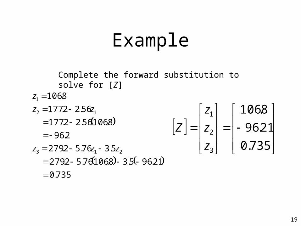
Example
19
Complete the forward substitution to solve for [Z]
735.0
21.965.38.10676.52.279
5.376.52.279
2.96
8.10656.22.177
56.22.177
8.106
213
12
1
zzz
zz
z
735.0
21.96
8.106
3
2
1
z
z
z
Z
Example
735.07.0
21.9656.18.4
8.106525
3
32
321
a
aa
aaa
20
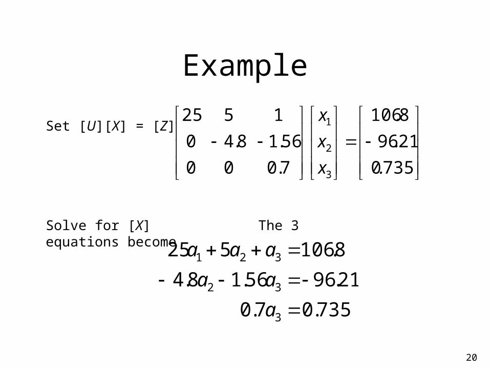
Set [U][X] = [Z]
Solve for [X] The 3 equations become
7350
2196
8106
7.000
56.18.40
1525
3
2
1
.
.
.
x
x
x
Example
21
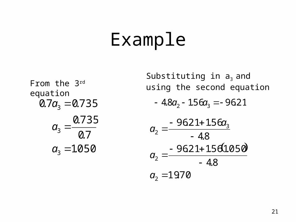
From the 3rd equation
050170
7350
735070
3
3
3
.a.
.a
.a.
Substituting in a3 and using the second equation
219656184 32 .a.a.
701984
0501561219684
5612196
2
2
32
.a.
...a
.
a..a

Example
22
Substituting in a3 and a2 using the first equation
8106525 321 .aaa
Hence the Solution Vector is:
050.1
70.19
2900.0
3
2
1
a
a
a
2900025
050170195810625
58106 321
.
...
aa.a
Finding the inverse of a square matrix
23
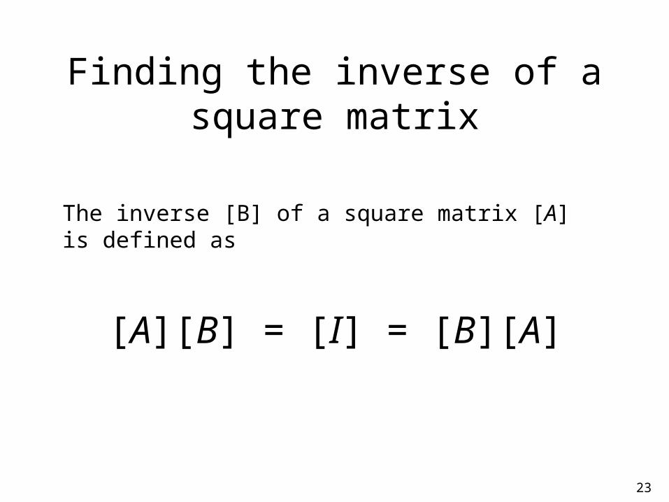
The inverse [B] of a square matrix [A] is defined as
[A][B] = [I] = [B][A]
Finding the inverse of a square matrix
24
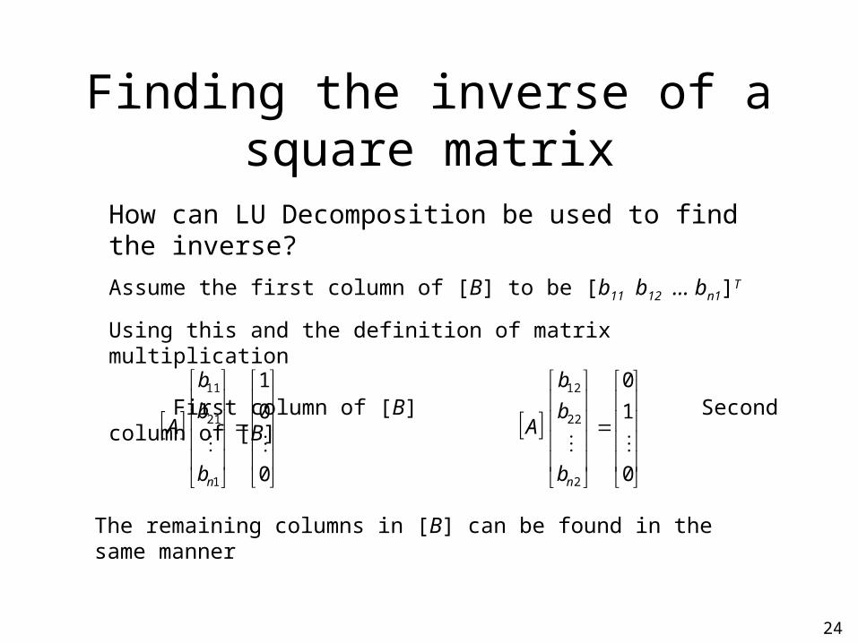
How can LU Decomposition be used to find the inverse?
Assume the first column of [B] to be [b11 b12 … bn1]T
Using this and the definition of matrix multiplication
First column of [B] Second column of [B]
0
0
1
1
21
11
nb
b
b
A
0
1
0
2
22
12
nb
b
b
A
The remaining columns in [B] can be found in the same manner
Example: Inverse of a Matrix
25
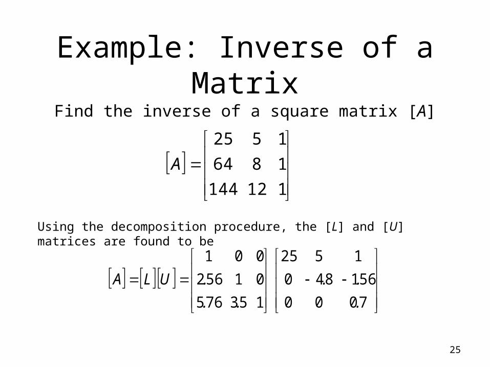
Find the inverse of a square matrix [A]
112144
1864
1525
A
7000
561840
1525
153765
01562
001
.
..
..
.ULA
Using the decomposition procedure, the [L] and [U] matrices are found to be

Example: Inverse of a Matrix
26
Solving for the each column of [B] requires two steps
1)Solve [L] [Z] = [C] for [Z]
2)Solve [U] [X] = [Z] for [X]
Step 1:
0
0
1
15.376.5
0156.2
001
3
2
1
z
z
z
CZL
This generates the equations:
05.376.5
056.2
1
321
21
1
zzz
zz
z

Example: Inverse of a Matrix
27
Solving for [Z]
23
5625317650
537650
562
15620
5620
1
213
12
1
.
...
z.z.z
.
.
z. z
z
23
562
1
3
2
1
.
.
z
z
z
Z
Example: Inverse of a Matrix
28
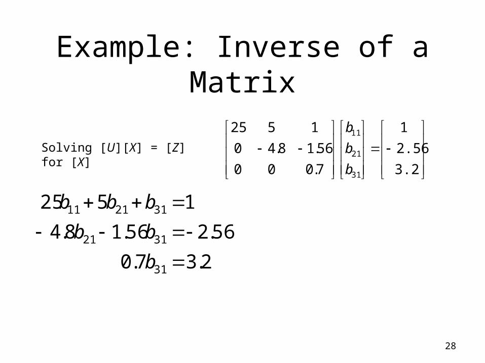
Solving [U][X] = [Z] for [X]
3.2
2.56
1
7.000
56.18.40
1525
31
21
11
b
b
b
2.37.0
56.256.18.4
1525
31
3121
312111
b
bb
bbb
Example: Inverse of a Matrix
29
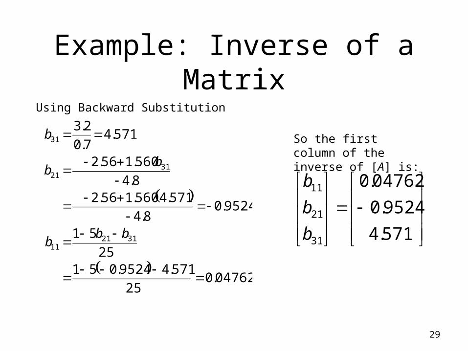
Using Backward Substitution
04762.0
25
571.49524.05125
51
9524.08.4
571.4560.156.28.4
560.156.2
571.47.0
2.3
312111
3121
31
bbb
bb
b So the first column of the inverse of [A] is:
571.4
9524.0
04762.0
31
21
11
b
b
b
Example: Inverse of a Matrix
30
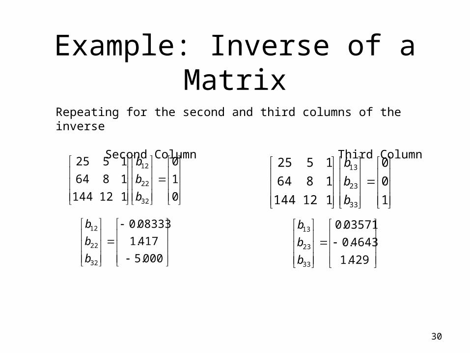
Repeating for the second and third columns of the inverse
Second Column Third Column
0
1
0
112144
1864
1525
32
22
12
b
b
b
000.5
417.1
08333.0
32
22
12
b
b
b
1
0
0
112144
1864
1525
33
23
13
b
b
b
429.1
4643.0
03571.0
33
23
13
b
b
b
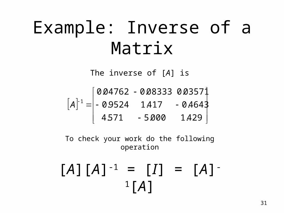
Example: Inverse of a Matrix
31
The inverse of [A] is
429.1000.5571.4
4643.0417.19524.0
03571.008333.004762.01A
To check your work do the following operation
[A][A]-1 = [I] = [A]-1[A]
32
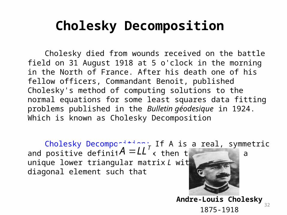
Cholesky Decomposition
Cholesky died from wounds received on the battle field on 31 August 1918 at 5 o'clock in the morning in the North of France. After his death one of his fellow officers, Commandant Benoit, published Cholesky's method of computing solutions to the normal equations for some least squares data fitting problems published in the Bulletin géodesique in 1924. Which is known as Cholesky Decomposition
Cholesky Decomposition: If A is a real, symmetric and
positive definite matrix then there exists a unique lower triangular matrix L with positive diagonal element such that .
TLLA
Andre-Louis Cholesky
1875-1918

Cholesky Factorization
• Symmetric systems occur commonly in both mathematical and engineering/science problem contexts, and there are special solution techniques available for such systems.
• The Cholesky factorization is one of the most popular of these techniques, and is based on the fact that a symmetric matrix can be decomposed as [A]= [U]T[U], where T stands for transpose.
• The rest of the process is similar to LU decomposition and Gauss elimination, except only one matrix, [U], needs to be stored.
33