Embed Size (px)
Citation preview
Ludovico Carrino
The weighting role of normalisation in a
multidimensional analysis of Social Inclusion
���ISSN: 1827-3580 No. 32/WP/2015
W o r k i n g P a p e r s D e p a r t m e n t o f E c o n o m i c s
C a ’ F o s c a r i U n i v e r s i t y o f V e n i c e N o . 3 2 / W P / 2 0 1 5
ISSN 1827-3580
The Working Paper Series is available only on line
(http://www.unive.it/nqcontent.cfm?a_id=86302) For editorial correspondence, please contact:
Department of Economics Ca’ Foscari University of Venice Cannaregio 873, Fondamenta San Giobbe 30121 Venice Italy Fax: ++39 041 2349210
The weighting role of normalisation in a multidimensional analysis of Social Inclusion
Ludovico Carrino Ca’ Foscari University of Venice
Abstract In the context of the multidimensional measurement of complex phenomena, the major focus of the recent literature has been on the choice of the dimensions’ weights and the shape of the aggregation function, while few studies have concentrated on how normalisation influences the results. With the aim of building a measure of Social Inclusion for European regions between 2004 and 2012, we adopt a CES aggregation framework and compare two alternative normalisation strategies: a data-driven min-max function, where the parameters depends solely on the available data, and an expert-based function where parameters are elicited through a survey at the University of Venice Ca’ Foscari. Regardless of the adopted strategy, we show that normalisation plays a crucial part in defining variables’ weighting and trade-offs. The data-driven strategy produces trade-offs that are hard to interpret in economic terms and debatable from a social desirability perspective, thus generating an aggregate measure with a “positive” interpretation. Moreover, it softens the aftermaths of the recent economic crisis on Social Inclusion, by putting a consistent weight on the longevity variable. Conversely, the expert-based normalisation has strikingly different parameters and allows for a normative interpretation of the resulting index. Furthermore, it emphasizes the worsening trends in long- term unemployment and the relevance of early school leaving in the Social Inclusion measure. As a result, numerous rank-reversals occur between regions when switching the normalisation methods.
Keywords CES, normalisation, aggregation, weighting, experts, multidimensionality, Social Inclusion
JEL Codes C43, C83, D63, I32
Address for correspondence: Ludovico Carrino
Department of Economics Ca’ Foscari University of Venice
Cannaregio 873, Fondamenta S.Giobbe 30121 Venezia - Italy
Phone: (++39) 041 2349140 Fax: (++39) 041 2349176 e-mail: [email protected]
This Working Paper is published under the auspices of the Department of Economics of the Ca’ Foscari University of Venice. Opinions expressed herein are those of the authors and not those of the Department. The Working Paper series is designed to divulge preliminary or
incomplete work, circulated to favour discussion and comments. Citation of this paper should consider its provisional character.
The weighting role of normalisation in a multidimensional analysis of Social Inclusion1
Ludovico Carrino (Economics Department, Ca’ Foscari University of Venice, Italy)
November 2015 Abstract In the context of the multidimensional measurement of complex phenomena, the major focus of the recent literature has been on the choice of the dimensions’ weights and the shape of the aggregation function, while few studies have concentrated on how normalisation influences the results. With the aim of building a measure of Social Inclusion for European regions between 2004 and 2012, we adopt a CES aggregation framework and compare two alternative normalisation strategies: a data-driven min-max function, where the parameters depends solely on the available data, and an expert-based function where parameters are elicited through a survey at the University of Venice Ca’Foscari. Regardless of the adopted strategy, we show that normalisation plays a crucial part in defining variables’ weighting and trade-offs. The data-driven strategy produces trade-offs that are hard to interpret in economic terms and debatable from a social desirability perspective, thus generating an aggregate measure with a “positive” interpretation. Moreover, it softens the aftermaths of the recent economic crisis on Social Inclusion, by putting a consistent weight on the longevity variable. Conversely, the expert-based normalisation has strikingly different parameters and allows for a normative interpretation of the resulting index. Furthermore, it emphasizes the worsening trends in long-term unemployment and the relevance of early school leaving in the Social Inclusion measure. As a result, numerous rank-reversals occur between regions when switching the normalisation methods.
JEL categories: C43, C83, D63, I32
Keywords: CES, normalisation, aggregation, weighting, experts, multidimensionality, Social Inclusion Address for correspondence: Ludovico Carrino, Department of Economics, Ca’ Foscari University of Venice, Cannaregio 873, Fondamenta S.Giobbe, 30121 Venezia – Italy, Phone: (++39) 041 2349140, Fax: (++39) 041 2349176, e-mail: [email protected]
1 The author wishes to thank Michele Bernasconi, Giovanni Bertin, Eric Bonsang, Agar Brugiavini, Stefano Campostrini, Roberto Casarin, Koen Decanq, Silvio Giove, Filomena Maggino, Sergio Perelman, Pierre Pestieau, Dino Rizzi, Maurizio Zenezini, for their valuable comments to previous versions of this paper. The paper benefited as well from comments by participants to seminars at Ca’ Foscari University of Venice, University of Trieste, as well as to the conference “Complexity in Society” at University of Padova. The authors acknowledge the financial support of Fondazione Ca’ Foscari.
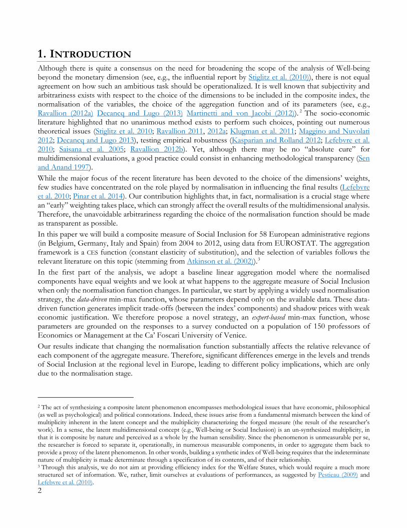
1. INTRODUCTION Although there is quite a consensus on the need for broadening the scope of the analysis of Well-being beyond the monetary dimension (see, e.g., the influential report by Stiglitz et al. (2010)), there is not equal agreement on how such an ambitious task should be operationalized. It is well known that subjectivity and arbitrariness exists with respect to the choice of the dimensions to be included in the composite index, the normalisation of the variables, the choice of the aggregation function and of its parameters (see, e.g., Ravallion (2012a) Decancq and Lugo (2013) Martinetti and von Jacobi (2012)). 2 The socio-economic literature highlighted that no unanimous method exists to perform such choices, pointing out numerous theoretical issues (Stiglitz et al. 2010; Ravallion 2011, 2012a; Klugman et al. 2011; Maggino and Nuvolati 2012; Decancq and Lugo 2013), testing empirical robustness (Kasparian and Rolland 2012; Lefebvre et al. 2010; Saisana et al. 2005; Ravallion 2012b). Yet, although there may be no “absolute cure” for multidimensional evaluations, a good practice could consist in enhancing methodological transparency (Sen and Anand 1997). While the major focus of the recent literature has been devoted to the choice of the dimensions’ weights, few studies have concentrated on the role played by normalisation in influencing the final results (Lefebvre et al. 2010; Pinar et al. 2014). Our contribution highlights that, in fact, normalisation is a crucial stage where an “early” weighting takes place, which can strongly affect the overall results of the multidimensional analysis. Therefore, the unavoidable arbitrariness regarding the choice of the normalisation function should be made as transparent as possible. In this paper we will build a composite measure of Social Inclusion for 58 European administrative regions (in Belgium, Germany, Italy and Spain) from 2004 to 2012, using data from EUROSTAT. The aggregation framework is a CES function (constant elasticity of substitution), and the selection of variables follows the relevant literature on this topic (stemming from Atkinson et al. (2002)).3 In the first part of the analysis, we adopt a baseline linear aggregation model where the normalised components have equal weights and we look at what happens to the aggregate measure of Social Inclusion when only the normalisation function changes. In particular, we start by applying a widely used normalisation strategy, the data-driven min-max function, whose parameters depend only on the available data. These data-driven function generates implicit trade-offs (between the index’ components) and shadow prices with weak economic justification. We therefore propose a novel strategy, an expert-based min-max function, whose parameters are grounded on the responses to a survey conducted on a population of 150 professors of Economics or Management at the Ca’ Foscari University of Venice. Our results indicate that changing the normalisation function substantially affects the relative relevance of each component of the aggregate measure. Therefore, significant differences emerge in the levels and trends of Social Inclusion at the regional level in Europe, leading to different policy implications, which are only due to the normalisation stage.
2 The act of synthesizing a composite latent phenomenon encompasses methodological issues that have economic, philosophical (as well as psychological) and political connotations. Indeed, these issues arise from a fundamental mismatch between the kind of multiplicity inherent in the latent concept and the multiplicity characterizing the forged measure (the result of the researcher’s work). In a sense, the latent multidimensional concept (e.g., Well-being or Social Inclusion) is an un-synthesized multiplicity, in that it is composite by nature and perceived as a whole by the human sensibility. Since the phenomenon is unmeasurable per se, the researcher is forced to separate it, operationally, in numerous measurable components, in order to aggregate them back to provide a proxy of the latent phenomenon. In other words, building a synthetic index of Well-being requires that the indeterminate nature of multiplicity is made determinate through a specification of its contents, and of their relationship. 3 Through this analysis, we do not aim at providing efficiency index for the Welfare States, which would require a much more structured set of information. We, rather, limit ourselves at evaluations of performances, as suggested by Pestieau (2009) and Lefebvre et al. (2010). 2
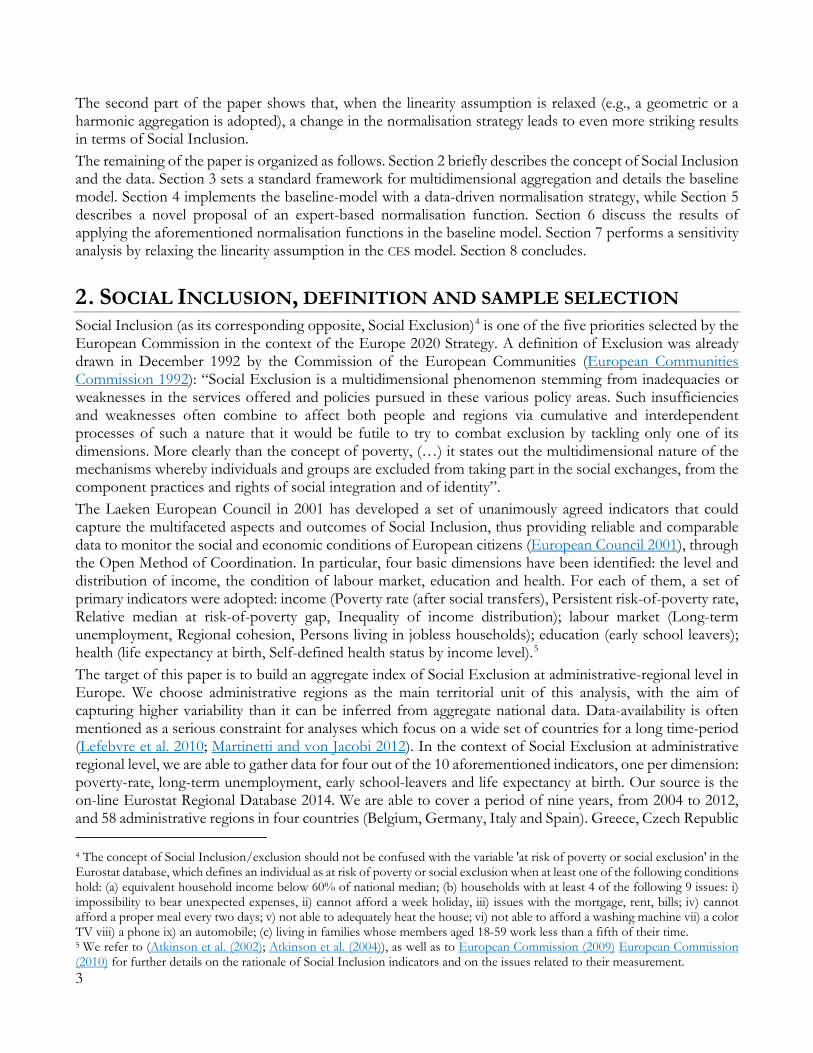
The second part of the paper shows that, when the linearity assumption is relaxed (e.g., a geometric or a harmonic aggregation is adopted), a change in the normalisation strategy leads to even more striking results in terms of Social Inclusion. The remaining of the paper is organized as follows. Section 2 briefly describes the concept of Social Inclusion and the data. Section 3 sets a standard framework for multidimensional aggregation and details the baseline model. Section 4 implements the baseline-model with a data-driven normalisation strategy, while Section 5 describes a novel proposal of an expert-based normalisation function. Section 6 discuss the results of applying the aforementioned normalisation functions in the baseline model. Section 7 performs a sensitivity analysis by relaxing the linearity assumption in the CES model. Section 8 concludes.
2. SOCIAL INCLUSION, DEFINITION AND SAMPLE SELECTION Social Inclusion (as its corresponding opposite, Social Exclusion)4 is one of the five priorities selected by the European Commission in the context of the Europe 2020 Strategy. A definition of Exclusion was already drawn in December 1992 by the Commission of the European Communities (European Communities Commission 1992): “Social Exclusion is a multidimensional phenomenon stemming from inadequacies or weaknesses in the services offered and policies pursued in these various policy areas. Such insufficiencies and weaknesses often combine to affect both people and regions via cumulative and interdependent processes of such a nature that it would be futile to try to combat exclusion by tackling only one of its dimensions. More clearly than the concept of poverty, (…) it states out the multidimensional nature of the mechanisms whereby individuals and groups are excluded from taking part in the social exchanges, from the component practices and rights of social integration and of identity”. The Laeken European Council in 2001 has developed a set of unanimously agreed indicators that could capture the multifaceted aspects and outcomes of Social Inclusion, thus providing reliable and comparable data to monitor the social and economic conditions of European citizens (European Council 2001), through the Open Method of Coordination. In particular, four basic dimensions have been identified: the level and distribution of income, the condition of labour market, education and health. For each of them, a set of primary indicators were adopted: income (Poverty rate (after social transfers), Persistent risk-of-poverty rate, Relative median at risk-of-poverty gap, Inequality of income distribution); labour market (Long-term unemployment, Regional cohesion, Persons living in jobless households); education (early school leavers); health (life expectancy at birth, Self-defined health status by income level).5 The target of this paper is to build an aggregate index of Social Exclusion at administrative-regional level in Europe. We choose administrative regions as the main territorial unit of this analysis, with the aim of capturing higher variability than it can be inferred from aggregate national data. Data-availability is often mentioned as a serious constraint for analyses which focus on a wide set of countries for a long time-period (Lefebvre et al. 2010; Martinetti and von Jacobi 2012). In the context of Social Exclusion at administrative regional level, we are able to gather data for four out of the 10 aforementioned indicators, one per dimension: poverty-rate, long-term unemployment, early school-leavers and life expectancy at birth. Our source is the on-line Eurostat Regional Database 2014. We are able to cover a period of nine years, from 2004 to 2012, and 58 administrative regions in four countries (Belgium, Germany, Italy and Spain). Greece, Czech Republic
4 The concept of Social Inclusion/exclusion should not be confused with the variable 'at risk of poverty or social exclusion' in the Eurostat database, which defines an individual as at risk of poverty or social exclusion when at least one of the following conditions hold: (a) equivalent household income below 60% of national median; (b) households with at least 4 of the following 9 issues: i) impossibility to bear unexpected expenses, ii) cannot afford a week holiday, iii) issues with the mortgage, rent, bills; iv) cannot afford a proper meal every two days; v) not able to adequately heat the house; vi) not able to afford a washing machine vii) a color TV viii) a phone ix) an automobile; (c) living in families whose members aged 18-59 work less than a fifth of their time. 5 We refer to (Atkinson et al. (2002); Atkinson et al. (2004)), as well as to European Commission (2009) European Commission (2010) for further details on the rationale of Social Inclusion indicators and on the issues related to their measurement. 3
and Norway were not included in the sample since their data are made available for statistical-regions, but not for administrative regions. As argued in Lefebvre et al. (2010), “these indicators cover the most relevant concerns of a modern welfare state, also reflecting aspects that people who want to enlarge the concept of GDP to better measure social welfare generally take into account”. The latter referenced paper, as do Atkinson et al. (2004), discusses the limitations of these data and the necessary simplifying assumptions that have to be done when translating a complex multidimensional phenomenon like Social Exclusion in empirical terms. Table 2-1 provides a brief definition for our four variables: Table 2-1, Variable definitions
variable definition Poverty rate Share of individuals living in households with an income below 60% national median
equivalised disposable income. Long-term unemployment rate Total long-term unemployed population (≥12 months; ILO definition) as proportion
of total active population. Early school-leavers Share of total population of 18-24-year olds having achieved ISCED level 2 or less
and not attending education or training. Life expectancy at birth Number of years a person may be expected to live, starting at age 0.
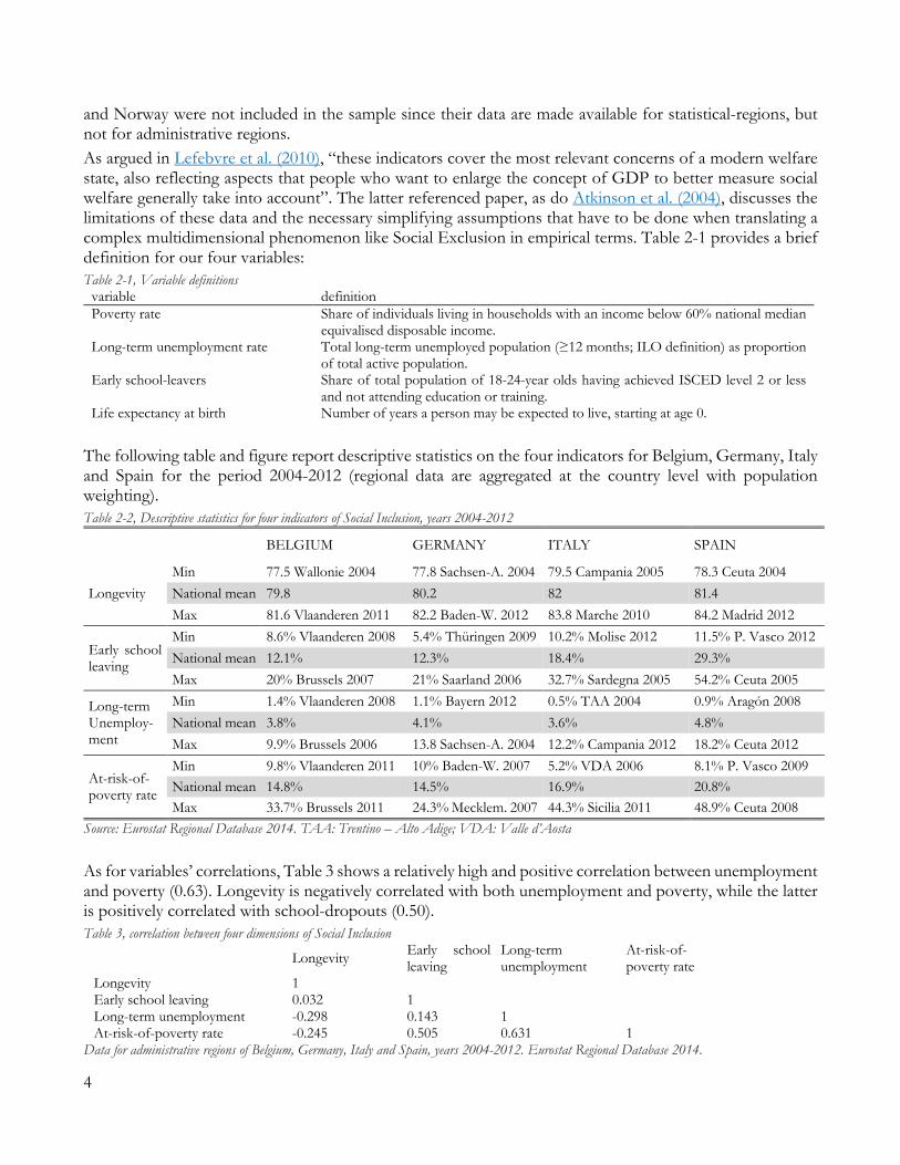
The following table and figure report descriptive statistics on the four indicators for Belgium, Germany, Italy and Spain for the period 2004-2012 (regional data are aggregated at the country level with population weighting). Table 2-2, Descriptive statistics for four indicators of Social Inclusion, years 2004-2012
BELGIUM GERMANY ITALY SPAIN
Longevity Min 77.5 Wallonie 2004 77.8 Sachsen-A. 2004 79.5 Campania 2005 78.3 Ceuta 2004 National mean 79.8 80.2 82 81.4 Max 81.6 Vlaanderen 2011 82.2 Baden-W. 2012 83.8 Marche 2010 84.2 Madrid 2012
Early school leaving
Min 8.6% Vlaanderen 2008 5.4% Thüringen 2009 10.2% Molise 2012 11.5% P. Vasco 2012 National mean 12.1% 12.3% 18.4% 29.3% Max 20% Brussels 2007 21% Saarland 2006 32.7% Sardegna 2005 54.2% Ceuta 2005
Long-term Unemploy-ment
Min 1.4% Vlaanderen 2008 1.1% Bayern 2012 0.5% TAA 2004 0.9% Aragón 2008 National mean 3.8% 4.1% 3.6% 4.8% Max 9.9% Brussels 2006 13.8 Sachsen-A. 2004 12.2% Campania 2012 18.2% Ceuta 2012
At-risk-of-poverty rate
Min 9.8% Vlaanderen 2011 10% Baden-W. 2007 5.2% VDA 2006 8.1% P. Vasco 2009 National mean 14.8% 14.5% 16.9% 20.8% Max 33.7% Brussels 2011 24.3% Mecklem. 2007 44.3% Sicilia 2011 48.9% Ceuta 2008
Source: Eurostat Regional Database 2014. TAA: Trentino – Alto Adige; VDA: Valle d’Aosta As for variables’ correlations, Table 3 shows a relatively high and positive correlation between unemployment and poverty (0.63). Longevity is negatively correlated with both unemployment and poverty, while the latter is positively correlated with school-dropouts (0.50). Table 3, correlation between four dimensions of Social Inclusion
Longevity Early school leaving
Long-term unemployment
At-risk-of-poverty rate
Longevity 1 Early school leaving 0.032 1 Long-term unemployment -0.298 0.143 1 At-risk-of-poverty rate -0.245 0.505 0.631 1
Data for administrative regions of Belgium, Germany, Italy and Spain, years 2004-2012. Eurostat Regional Database 2014.
4
3. THEORETICAL FRAMEWORK Let us consider m dimensions (hereinafter also variables, attributes, components) of Social Inclusion, observed for n territorial units (in our case, regions). For a generic region i we can therefore build the vector ( )1 , ...,
i i i
mx xx = ,
while X ×∈\n m is the distribution matrix of m attributes for n regions. To retrieve an aggregated measure for region i, we consider the function F defined as:
(1) 1
1 1 1
/i i i i
m m mF v w v x w v xxCC C ¯¡ °¢ ±� � �"
which can be referred to as a CES (constant elasticity of substitution) function, or a generalized mean of order β. Its arguments are the elements v1, …, vm which are transformations of the original variables x1,…,xm (defined hereafter). The function F is non-decreasing, separable, weakly scale-invariant and homogenous of degree-one in its arguments v; we refer to Blackorby and Donaldson (1982) and (Decancq and Lugo (2009), 2008)) for an analytic characterization of these properties. The parameters w1,…,wm , the weights of the normalised dimensions v, are non-negative and sum to one. Provided that a choice of the m dimension has been performed, the main methodological task is now the selection of the set of functions v1,…,vm , of parameters w1,…wm, as well as of β.
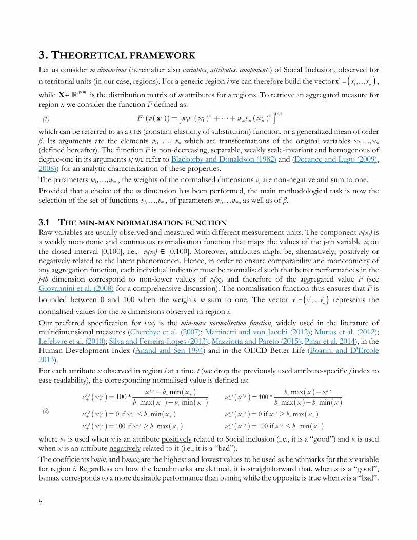
3.1 THE MIN-MAX NORMALISATION FUNCTION Raw variables are usually observed and measured with different measurement units. The component vi(xj) is a weakly monotonic and continuous normalisation function that maps the values of the j-th variable xj on the closed interval [0,100], i.e., vj(xj) ∈ [0,100]. Moreover, attributes might be, alternatively, positively or negatively related to the latent phenomenon. Hence, in order to ensure comparability and monotonicity of any aggregation function, each individual indicator must be normalised such that better performances in the j-th dimension correspond to non-lower values of vj(xj) and therefore of the aggregated value F (see Giovannini et al. (2008) for a comprehensive discussion). The normalisation function thus ensures that F is bounded between 0 and 100 when the weights w sum to one. The vector ( )1
, ...,i i i
mv vv = represents the
normalised values for the m dimensions observed in region i. Our preferred specification for v(x) is the min-max normalisation function, widely used in the literature of multidimensional measures (Cherchye et al. (2007); Martinetti and von Jacobi (2012); Murias et al. (2012); Lefebvre et al. (2010); Silva and Ferreira-Lopes (2013); Mazziotta and Pareto (2015); Pinar et al. 2014), in the Human Development Index (Anand and Sen 1994) and in the OECD Better Life (Boarini and D'Ercole 2013). For each attribute x observed in region i at a time t (we drop the previously used attribute-specific j index to ease readability), the corresponding normalised value is defined as:
(2)
,
, ,
, ,
,,
,
,
0 if min100 if max
min100 * max mini t
i t i t
i t i t
i ti t
i t
i t
x b xx b x
x b xx b x b xxx
O
O
O
� ��
� � � �
� � � �
� � � �
�
�
�
� b
� p
��
�
, ,
, ,
,, ,
,
,
100 *
0 if max100 if min
maxmax min
i t i t
i t i t
i ti t i t
i t
i t
x b xx b x
b x xx b x b xxx
O
O
O
�
� �
� � � �
� � � �
�
�
�
�
� p
� b
��
where ν+ is used when x is an attribute positively related to Social inclusion (i.e., it is a “good”) and ν- is used when x is an attribute negatively related to it (i.e., it is a “bad”). The coefficients bmini and bmaxi are the highest and lowest values to be used as benchmarks for the x variable for region i. Regardless on how the benchmarks are defined, it is straightforward that, when x is a “good”, b+max corresponds to a more desirable performance than b+min, while the opposite is true when x is a “bad”.
5
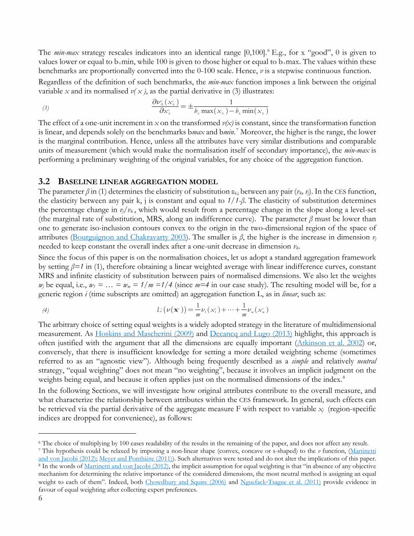
The min-max strategy rescales indicators into an identical range [0,100].6 E.g., for x “good”, 0 is given to values lower or equal to b+min, while 100 is given to those higher or equal to b+max. The values within these benchmarks are proportionally converted into the 0-100 scale. Hence, ν is a stepwise continuous function. Regardless of the definition of such benchmarks, the min-max function imposes a link between the original variable x and its normalised ν( x ), as the partial derivative in (3) illustrates:
(3)
1
max mini
i
i xx b x b x
O o
o o o o o
os�o
s �
The effect of a one-unit increment in x on the transformed ν(x) is constant, since the transformation function is linear, and depends solely on the benchmarks bmax and bmin.7 Moreover, the higher is the range, the lower is the marginal contribution. Hence, unless all the attributes have very similar distributions and comparable units of measurement (which would make the normalisation itself of secondary importance), the min-max is performing a preliminary weighting of the original variables, for any choice of the aggregation function.
3.2 BASELINE LINEAR AGGREGATION MODEL The parameter β in (1) determines the elasticity of substitution εk,j between any pair (vk, vj). In the CES function, the elasticity between any pair k, j is constant and equal to 1/1-β. The elasticity of substitution determines the percentage change in vj/vk , which would result from a percentage change in the slope along a level-set (the marginal rate of substitution, MRS, along an indifference curve). The parameter β must be lower than one to generate iso-inclusion contours convex to the origin in the two-dimensional region of the space of attributes (Bourguignon and Chakravarty 2003). The smaller is β, the higher is the increase in dimension vj needed to keep constant the overall index after a one-unit decrease in dimension vk. Since the focus of this paper is on the normalisation choices, let us adopt a standard aggregation framework by setting β=1 in (1), therefore obtaining a linear weighted average with linear indifference curves, constant MRS and infinite elasticity of substitution between pairs of normalised dimensions. We also let the weights wj be equal, i.e., w1 = … = wm = 1/m =1/4 (since m=4 in our case study). The resulting model will be, for a generic region i (time subscripts are omitted) an aggregation function L, as in linear, such as:
(4) 1 1
1 1i i i i
m mL x xm m
O O O� ��x "
The arbitrary choice of setting equal weights is a widely adopted strategy in the literature of multidimensional measurement. As Hoskins and Mascherini (2009) and Decancq and Lugo (2013) highlight, this approach is often justified with the argument that all the dimensions are equally important (Atkinson et al. 2002) or, conversely, that there is insufficient knowledge for setting a more detailed weighting scheme (sometimes referred to as an “agnostic view”). Although being frequently described as a simple and relatively neutral strategy, “equal weighting” does not mean “no weighting”, because it involves an implicit judgment on the weights being equal, and because it often applies just on the normalised dimensions of the index.8 In the following Sections, we will investigate how original attributes contribute to the overall measure, and what characterize the relationship between attributes within the CES framework. In general, such effects can be retrieved via the partial derivative of the aggregate measure F with respect to variable xj (region-specific indices are dropped for convenience), as follows:
6 The choice of multiplying by 100 eases readability of the results in the remaining of the paper, and does not affect any result. 7 This hypothesis could be relaxed by imposing a non-linear shape (convex, concave or s-shaped) to the ν function, (Martinetti and von Jacobi (2012); Meyer and Ponthière (2011)). Such alternatives were tested and do not alter the implications of this paper. 8 In the words of Martinetti and von Jacobi (2012), the implicit assumption for equal weighting is that “in absence of any objective mechanism for determining the relative importance of the considered dimensions, the most neutral method is assigning an equal weight to each of them”. Indeed, both Chowdhury and Squire (2006) and Nguefack-Tsague et al. (2011) provide evidence in favour of equal weighting after collecting expert preferences. 6
(5)
11
1 1 1
11 11 1 1
1x
x/
m m m j j j j jj
m m mj j j j j j
j j j j
F v w v x w v x w v x v xxw v x w v x F vw v x w v x
v x v x
CCC C C
CC CC C
CC
��
��
¯¡ °¢ ±� ¬ ¯ � ¬� ¡ ° �� ¢ ± �� �� �� � ®�� ®
s a� � �s
� �a a� �
"
"
From (5) we can identify four main drivers that determine how the aggregate measure F reacts at small changes in the j-th real-valued dimension xj. The higher is the weight of the normalised j-th dimension, the higher will be the marginal variation in the F. The steeper is the normalisation function, the higher will be the effect of a change in the j-th dimension on the aggregate measure. The worse is the starting condition in the j-th dimension with respect to the aggregate measure, the higher will be its marginal contribution. Finally, the lower is the degree of substitutability β, the more sensitive F will be to bad performances in the j-th attribute. Within the aggregation function F, the marginal rate of substitution between a pair of observed-indicators xj and xk is:
(6)
1
1
1
xx
x x, jk
j jk kj k k k kk kkx x
j jk k kj j j j
jj j
F vF vv xv xdx v x v xw wxMRS dx w w v xF v v x v xF v
x v x
C
C
C
�
�
�
� ¬� � � ¬� � ® � � � �� ¬ � ®� � � �� ®
sa as�� � � �
s a as
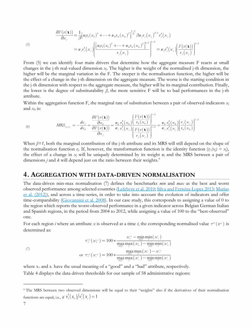
When β=1, both the marginal contribution of the j-th attribute and its MRS will still depend on the shape of the normalisation function vj. If, however, the transformation function is the identity function (vj (xj) = xj), the effect of a change in xj will be uniquely determined by its weight wj and the MRS between a pair of dimensions j and k will depend just on the ratio between their weights.9
4. AGGREGATION WITH DATA-DRIVEN NORMALISATION The data-driven min-max normalisation (7) defines the benchmarks min and max as the best and worst observed performance among selected countries (Lefebvre et al. 2010; Silva and Ferreira-Lopes 2013; Murias et al. (2012)), and across a time-series, in order to take into account the evolution of indicators and offer time-comparability (Giovannini et al. 2008). In our case study, this corresponds to assigning a value of 0 to the region which reports the worst-observed performance in a given indicator across Belgian German Italian and Spanish regions, in the period from 2004 to 2012, while assigning a value of 100 to the “best-observed” one. For each region i where an attribute x is observed at a time t, the corresponding normalised value , ,U i t i tx is determined as:
(7)
U
U
� �
�� �
� �
�� �
��
��
��
��
�� �
�
�� �
�
,
,
,
,
,
,
or
min min100 maxmax min min
maxmax100 maxmax min min
i t t
i tt t
t i t
i tt t
it Ti t
it Tit T
it Ti t
it Tit T
x xx x x
x xx x x
where x+ and x- have the usual meaning of a “good” and a “bad” attribute, respectively. Table 4 displays the data-driven thresholds for our sample of 58 administrative regions:
9 The MRS between two observed dimensions will be equal to their “weights” also if the derivatives of their normalisation
functions are equal, i.e., if 1k k j jv x v xa a � 7
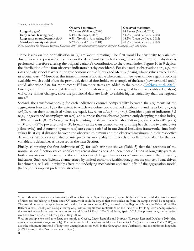
Table 4, data-driven benchmarks Observed minimum Observed maximum Longevity (good) 77.5 years (Wallonie, 2004) 84.2 years (Madrid, 2012) Early school leaving (bad) 5.4% (Thüringen, 2009) 54.2% (Ciutat de Ceuta, 2005) Long-term unemployment (bad) 0.5% (Trentino–Alto Adige, 2004) 18.2% (Ciutat de Ceuta, 2012) At-risk-of-poverty rate (bad) 5.2% (Valle d’Aosta, 2004) 48.9% (Ciutat de Ceuta, 2008)
Note: data from the Eurostat Regional Database 2014, for administrative regions in Belgium, Germany, Italy and Spain. Three issues on the normalisation in (7) are worth stressing. The first would be sensitivity to variables’ distribution: the presence of outliers in the data would stretch the range over which the normalisation is performed, therefore altering the original variable‘s contribution to the overall index. Figure 10 in 0 depicts the distribution of the four observed indicators hereby considered. Possible outlier observations are, e.g., the rates of early school leavers in the autonomous cities of Ceuta and Medilla (Spain), whose values exceed 45% in several years.10 Moreover, this transformation is not stable when data for new years or new regions become available, which could affect the previously defined thresholds. An example of the latter (new territorial units) could arise when data for more recent EU member states are added to the sample (Lefebvre et al. 2010). Finally, a shift in the territorial dimension of the analysis (e.g., from a regional to a provincial-level analysis) will cause similar changes, since the provincial data are likely to exhibit higher variability than the regional ones.11 Second, the transformations τj for each indicator j ensures comparability between the arguments of the aggregation function F, to the extent to which we define two observed attributes xj and xk as being equally satisfied when their normalised values are equal, i.e., when τj ( xj ) = τk ( xk ). Consider a pair of indicators j, k (e.g., longevity and unemployment rate), and suppose that we observe (conveniently dropping the time index) xj=81 years and xk=27% poverty rate. Implementing the data-driven transformation (7), leads us to τj (81 years) = 50 and τk (27% poverty-rate) = 50. Equality in the transformed values τj , τk implies that the two attributes j (longevity) and k (unemployment-rate) are equally satisfied in our Social Inclusion framework, since both values lie at equal distance between the observed-minimum and the observed-maximum in their respective data-series. Whether it can also be interpreted as an equality in the levels of welfare “revealed” by the two variables, is debatable, as discussed in the next Section. Finally, computing the first derivative of (7) for each attribute shows (Table 5) that the steepness of the normalisation function varies significantly across dimensions. An increment of 1 unit in longevity-years-at-birth translates in an increase for the τ function much larger than it does a 1-unit increment the remaining indicators. Such coefficients, characterized by limited economic justification, given the choice of data-driven benchmarks, will still inevitably affect the underlying mechanism and trade-offs of the aggregation model (hence, of its implicit preference structure).
10 Since these territories are substantially different from other Spanish regions (they are both located on the Mediterranean coast of Morocco but belong to Spain since XV century), it could be argued that their exclusion from the sample would be acceptable. This would decrease the upper bound of the distribution to a rate of 43%, reported by the Region of Murcia in 2004 and the Illes Balears in 2007, 2008 (both are Spanish regions), without significant implications on the trade-offs. For long-term unemployment, this exclusion would reduce the maximum bound from 18.2% to 15% (Andalucia, Spain, 2012. For poverty rate, the reduction would be from 48.9% to 44.5% (Sicilia, Italy, 2006). 11 As an example, we tried to enlarge the sample to Greece, Czech Republic and Norway (Eurostat Regional Database 2014, data available for statistical-regions only). The minimum level of early-school-leavers lowers to 1.8% (the Czech area Praha, 2006), as does the minimum threshold of long-term unemployment (to 0.3% in the Norwegian area Vestlandet), and the minimum longevity (to 74.2 years, in the Czech area Severozápad). 8
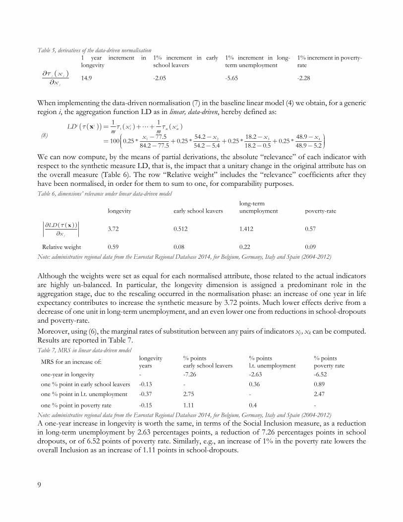
Table 5, derivatives of the data-driven normalisation 1 year increment in
longevity 1% increment in early school leavers
1% increment in long-term unemployment
1% increment in poverty-rate
j j
j
xx
Uss
14.9 -2.05 -5.65 -2.28
When implementing the data-driven normalisation (7) in the baseline linear model (4) we obtain, for a generic region i, the aggregation function LD as in linear, data-driven, hereby defined as:
(8) 1 1
1 2 3 4
1 1
77.5 54.2 18.2 48.9100 0.25 * 0.25 * 0.25 * 0.25 *84.2 77.5 54.2 5.4 18.2 0.5 48.9 5.2
i i i im mLD x x
m mx x x x
U U U� �
� � � �� ¬�� � � � � �� ®� � � �
� "x
We can now compute, by the means of partial derivations, the absolute “relevance” of each indicator with respect to the synthetic measure LD, that is, the impact that a unitary change in the original attribute has on the overall measure (Table 6). The row “Relative weight” includes the “relevance” coefficients after they have been normalised, in order for them to sum to one, for comparability purposes. Table 6, dimensions’ relevance under linear data-driven model
longevity early school leavers
long-term unemployment poverty-rate
j
LDx
xUss
3.72 0.512 1.412 0.57
Relative weight 0.59 0.08 0.22 0.09 Note: administrative regional data from the Eurostat Regional Database 2014, for Belgium, Germany, Italy and Spain (2004-2012) Although the weights were set as equal for each normalised attribute, those related to the actual indicators are highly un-balanced. In particular, the longevity dimension is assigned a predominant role in the aggregation stage, due to the rescaling occurred in the normalisation phase: an increase of one year in life expectancy contributes to increase the synthetic measure by 3.72 points. Much lower effects derive from a decrease of one unit in long-term unemployment, and an even lower one from reductions in school-dropouts and poverty-rate. Moreover, using (6), the marginal rates of substitution between any pairs of indicators xj , xk can be computed. Results are reported in Table 7. Table 7, MRS in linear data-driven model
MRS for an increase of: longevity years
% points early school leavers
% points l.t. unemployment
% points poverty rate
one-year in longevity - -7.26 -2.63 -6.52 one % point in early school leavers -0.13 - 0.36 0.89 one % point in l.t. unemployment -0.37 2.75 - 2.47
one % point in poverty rate -0.15 1.11 0.4 - Note: administrative regional data from the Eurostat Regional Database 2014, for Belgium, Germany, Italy and Spain (2004-2012) A one-year increase in longevity is worth the same, in terms of the Social Inclusion measure, as a reduction in long-term unemployment by 2.63 percentages points, a reduction of 7.26 percentages points in school dropouts, or of 6.52 points of poverty rate. Similarly, e.g., an increase of 1% in the poverty rate lowers the overall Inclusion as an increase of 1.11 points in school-dropouts.
9
5. EXPERT-BASED NORMALISATION
5.1 COLLECTING EXPERTS’ PREFERENCES In a simple linear model with β=1 and wj =1/m for each j-th indicators, the crucial determinant of a dimension’s relevance relies heavily on the normalisation function, as visible from (5). If the normalisation function’s parameters are arbitrarily determined through a data-driven strategy, its implications in terms of dimensions’ relative weights and MRS have a mathematic interpretation, yet it is harder to determine what do they reflect in economic terms (Lefebvre et al. 2010). Indeed, a variable with transformed-value equal to “0” just implies it being “the last one”, or “the worst one” among the observed, which does not necessarily corresponds to an undesirable condition of Well-being. A similar reasoning, with opposite meaning, can be done for normalised values of “100”. In this respect, the data-driven normalisation appears as a tool for a positive- rather than a normative-analysis of observed performances. Yet, as already argued, the absence of economic value judgments does not prevent the rescaling from a potential lack of robustness due to data availability. An alternative to the data-driven normalisation would require to incorporate some value judgments (e.g., social preferences, policy targets, expert opinions, see Decancq and Lugo (2013), Mazziotta and Pareto (2015), Kim et al. (2015)) in the normalisation. This translates to linking the extreme values “0” and the “100” with, e.g., a certain definition of desirability, thus making the normalisation independent from the data. When an indicator lies above or below such fixed bounds, further variations do not contribute to the latent variable under study (see e.g., the discussion in Anand and Sen (1994), Klugman et al. (2011), Ravallion (2012b), Lefebvre et al. (2010) and Gidwitz et al. (2010)). A major example of fixed threshold is the Human Development Index that, since 1994, adopted “goalposts” as minimum and maximum values in the normalisation function. The interpretation behind these fixed thresholds relies on the belief that objective upper and lower bounds can be identified, defined as “subsistence” minimum or “satiation” points, beyond which additional increments would not contribute to the expansion of capabilities.12 Contrary to Human Development, Social Exclusion’s concept has been developed with reference to advanced industrialized economies, as are those of the European Union members. Therefore, rather than on “subsistence”, its focus is posed on the “unacceptability” and “undesirability” of living conditions, as in an enlarged definition of poverty. Accordingly, a positive threshold for each of our four social-inclusion attributes would refer to a “certainly desirable and favourable condition of Well-being”, to which a normalised value of 100 would correspond. Conversely, a negative threshold would refer to a “certainly undesirable and harmful conditions of Well-being”, corresponding to a normalised value of 0. In order to select the actual thresholds, we chose to elicit expert preferences through a survey, rather than pre-determine them in a top-down fashion. Following Chowdhury and Squire (2006) and Hoskins and Mascherini (2009), we intended to involve informed opinions and therefore selected the population of professors and researchers in the Departments of Economic and Management of the Ca’ Foscari University of Venice. Specifically, our population consisted of 149 professors (57 + 38 full or associate professors of Economics and Management, respectively; 29 +
12 In the worldwide perspective of Human Development, the minimum “subsistence” point for longevity-at-birth was set to 25 years old in 2009, with “satiation” threshold at 85. Literacy rates’ boundaries were set at 0% and 100%, as was the gross enrolment ratio, while GDP per capita was limited between 100$ and 40,000$. Among the changes made since 2010, the upper values were now set to observed maxima over the time series between 1980 and the most recent year available, while the lower bounds were set equal to subsistence minima (see UNDP (2010) and Klugman et al. (2011)).
10
25 assistant professors (ricercatore universitario) of Economics and Management, respectively)13. The survey was worded in Italian and conducted in electronic-form with the QUALTRICS software, a web-based tool that enables users to build custom surveys and distribute them via email.14 Participants were invited with an email including a link to take part to the on-line questionnaire on an anonymous basis. The Survey was structured as follows:
• An introductory section discussed the topics, the purpose and the contents of the survey. • Respondents were asked to select the variables (amongst the four described in Section 2) for which
they would be willing to perform an evaluation. • A randomization led the respondent to a page devoted to one of the selected variables. All pages
were homogeneously designed with a consistent phrasing. • The EUROSTAT definition of the variable at hand was offered, and descriptive statistics were shown
through a bar graph, for 25 European countries (years 2000 and 2012). • The main task of the survey was then detailed. Respondents should identify, according to their own
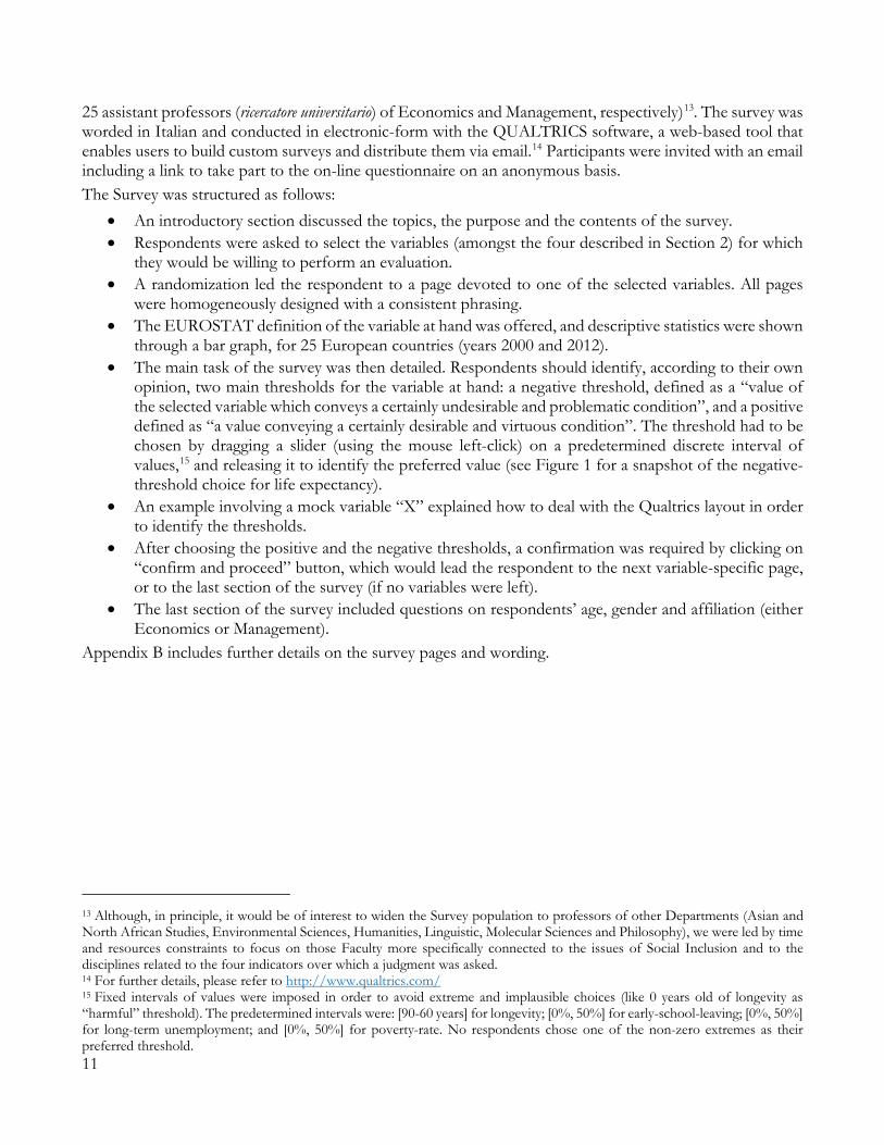
opinion, two main thresholds for the variable at hand: a negative threshold, defined as a “value of the selected variable which conveys a certainly undesirable and problematic condition”, and a positive defined as “a value conveying a certainly desirable and virtuous condition”. The threshold had to be chosen by dragging a slider (using the mouse left-click) on a predetermined discrete interval of values,15 and releasing it to identify the preferred value (see Figure 1 for a snapshot of the negative-threshold choice for life expectancy).
• An example involving a mock variable “X” explained how to deal with the Qualtrics layout in order to identify the thresholds.
• After choosing the positive and the negative thresholds, a confirmation was required by clicking on “confirm and proceed” button, which would lead the respondent to the next variable-specific page, or to the last section of the survey (if no variables were left).
• The last section of the survey included questions on respondents’ age, gender and affiliation (either Economics or Management).
Appendix B includes further details on the survey pages and wording.
13 Although, in principle, it would be of interest to widen the Survey population to professors of other Departments (Asian and North African Studies, Environmental Sciences, Humanities, Linguistic, Molecular Sciences and Philosophy), we were led by time and resources constraints to focus on those Faculty more specifically connected to the issues of Social Inclusion and to the disciplines related to the four indicators over which a judgment was asked. 14 For further details, please refer to http://www.qualtrics.com/ 15 Fixed intervals of values were imposed in order to avoid extreme and implausible choices (like 0 years old of longevity as “harmful” threshold). The predetermined intervals were: [90-60 years] for longevity; [0%, 50%] for early-school-leaving; [0%, 50%] for long-term unemployment; and [0%, 50%] for poverty-rate. No respondents chose one of the non-zero extremes as their preferred threshold. 11
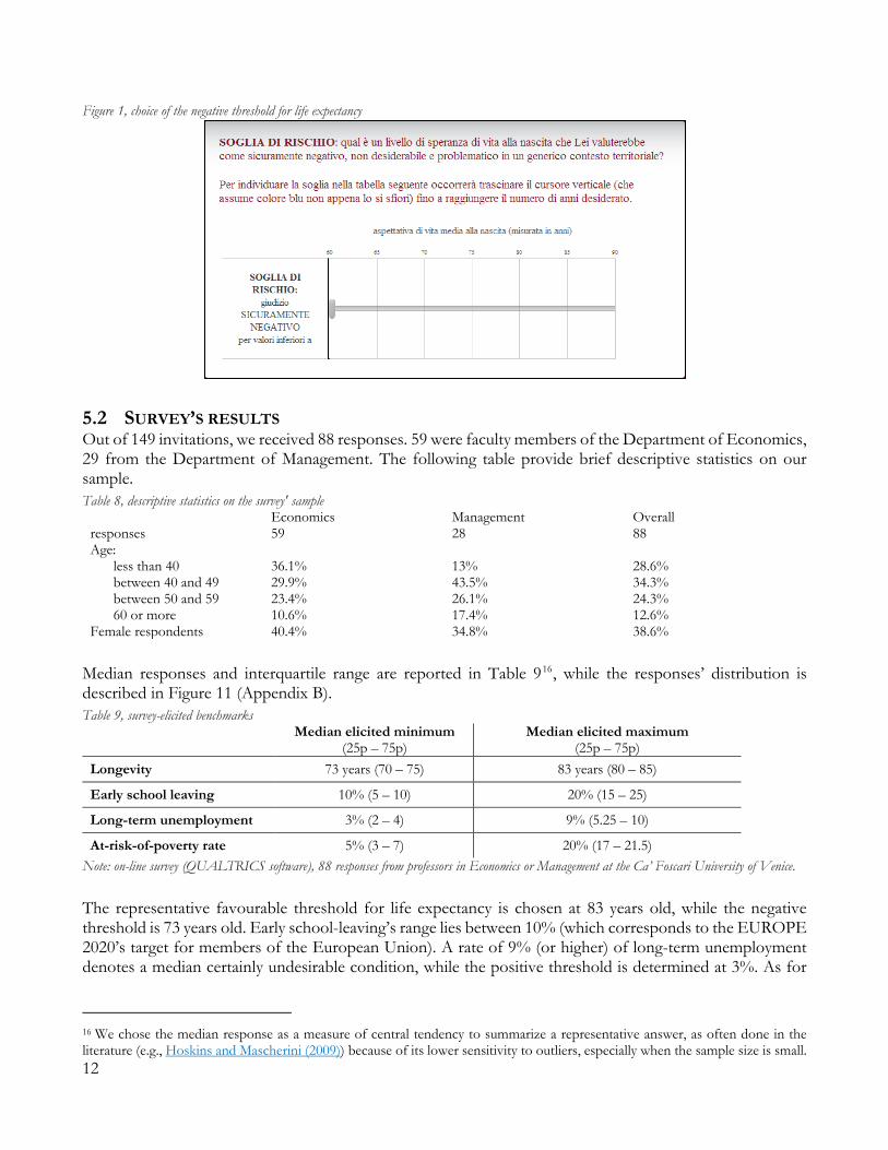
Figure 1, choice of the negative threshold for life expectancy
5.2 SURVEY’S RESULTS Out of 149 invitations, we received 88 responses. 59 were faculty members of the Department of Economics, 29 from the Department of Management. The following table provide brief descriptive statistics on our sample. Table 8, descriptive statistics on the survey' sample
Economics Management Overall responses 59 28 88 Age:
less than 40 36.1% 13% 28.6% between 40 and 49 29.9% 43.5% 34.3% between 50 and 59 23.4% 26.1% 24.3% 60 or more 10.6% 17.4% 12.6%
Female respondents 40.4% 34.8% 38.6% Median responses and interquartile range are reported in Table 916, while the responses’ distribution is described in Figure 11 (Appendix B). Table 9, survey-elicited benchmarks
Median elicited minimum (25p – 75p)
Median elicited maximum (25p – 75p)
Longevity 73 years (70 – 75) 83 years (80 – 85)
Early school leaving 10% (5 – 10) 20% (15 – 25)
Long-term unemployment 3% (2 – 4) 9% (5.25 – 10)
At-risk-of-poverty rate 5% (3 – 7) 20% (17 – 21.5) Note: on-line survey (QUALTRICS software), 88 responses from professors in Economics or Management at the Ca’ Foscari University of Venice. The representative favourable threshold for life expectancy is chosen at 83 years old, while the negative threshold is 73 years old. Early school-leaving’s range lies between 10% (which corresponds to the EUROPE 2020’s target for members of the European Union). A rate of 9% (or higher) of long-term unemployment denotes a median certainly undesirable condition, while the positive threshold is determined at 3%. As for
16 We chose the median response as a measure of central tendency to summarize a representative answer, as often done in the literature (e.g., Hoskins and Mascherini (2009)) because of its lower sensitivity to outliers, especially when the sample size is small. 12
poverty rate, a certainly harmful level has its median value at 20%, while desirability corresponds to 5% (or lower) share of population below the poverty line set by the Eurostat. The interquartile ranges are always relatively small, except for the negative threshold for early-school-leaving (15%-25%). Nevertheless, we are aware that no “true values” exist, with respect to these thresholds. In the words of Mascherini and Hoskins (2008), “the judgment of one of the outline may be correct, and those who share a consensus view may be wrong”. A quick comparison of Table 9 and Table 4 suggests that “certain desirability” and “certain undesirability” largely differ from observed minimum or maximum achievement. Indeed, a minimum observed level of longevity (77.5 years in Wallonia) is considered to be “certainly undesirable” by only a small fraction of respondents (Figure 11 in Appendix B). Similarly, any rate of long-term unemployment beyond 9%, or of school dropouts higher than 20%, or of poverty-rate beyond 20%, is regarded as certainly negative, while the actual observed maximums are quite higher. A capping on the positive threshold occurs for those regions which report long-term unemployment lower than 3% or early school leaving rates lower than 10%.17
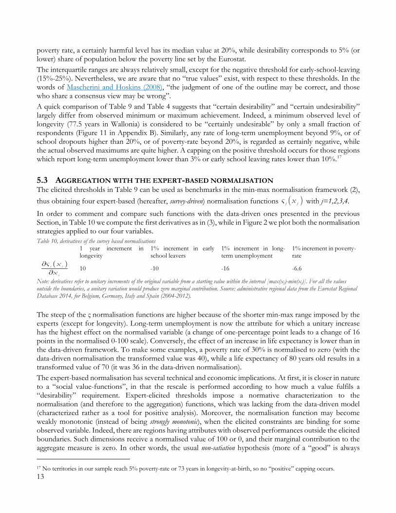
5.3 AGGREGATION WITH THE EXPERT-BASED NORMALISATION The elicited thresholds in Table 9 can be used as benchmarks in the min-max normalisation framework (2), thus obtaining four expert-based (hereafter, survey-driven) normalisation functions j jx7 with j=1,2,3,4. In order to comment and compare such functions with the data-driven ones presented in the previous Section, in Table 10 we compute the first derivatives as in (3), while in Figure 2 we plot both the normalisation strategies applied to our four variables. Table 10, derivatives of the survey based normalisations
1 year increment in longevity
1% increment in early school leavers
1% increment in long-term unemployment
1% increment in poverty-rate
j j
j
xx
7ss
10 -10 -16 -6.6
Note: derivatives refer to unitary increments of the original variable from a starting value within the interval [max(xj)-min(xj)]. For all the values outside the boundaries, a unitary variation would produce zero marginal contribution. Source: administrative regional data from the Eurostat Regional Database 2014, for Belgium, Germany, Italy and Spain (2004-2012). The steep of the ς normalisation functions are higher because of the shorter min-max range imposed by the experts (except for longevity). Long-term unemployment is now the attribute for which a unitary increase has the highest effect on the normalised variable (a change of one-percentage point leads to a change of 16 points in the normalised 0-100 scale). Conversely, the effect of an increase in life expectancy is lower than in the data-driven framework. To make some examples, a poverty rate of 30% is normalised to zero (with the data-driven normalisation the transformed value was 40), while a life expectancy of 80 years old results in a transformed value of 70 (it was 36 in the data-driven normalisation). The expert-based normalisation has several technical and economic implications. At first, it is closer in nature to a “social value-functions”, in that the rescale is performed according to how much a value fulfils a “desirability” requirement. Expert-elicited thresholds impose a normative characterization to the normalisation (and therefore to the aggregation) functions, which was lacking from the data-driven model (characterized rather as a tool for positive analysis). Moreover, the normalisation function may become weakly monotonic (instead of being strongly monotonic), when the elicited constraints are binding for some observed variable. Indeed, there are regions having attributes with observed performances outside the elicited boundaries. Such dimensions receive a normalised value of 100 or 0, and their marginal contribution to the aggregate measure is zero. In other words, the usual non-satiation hypothesis (more of a “good” is always
17 No territories in our sample reach 5% poverty-rate or 73 years in longevity-at-birth, so no “positive” capping occurs. 13
preferred to less) is maintained in a weaker form: more of a “good” is non-ill favoured with respect to less of it, after a certain performance is reached (and, conversely, more of a “bad” is non-preferred to less). As a rough realisation of the diminishing sensitivity hypothesis, the effects of a change in variables’ score on the social utility is zero, after the thresholds are crossed. From a policy-implication point of view, this suggests to focus on those dimensions whose performances lie farther away from the “desirability” level. 18 Figure 2, survey-driven vs data-driven normalisation
When implementing such normalisation function in the linear aggregation framework as in (4), we obtain, for a generic region i (time subscript are omitted) an aggregation function LS as in linear, survey-driven:
(9)
1 11
1 2 3 4
1 1 1 1 1 1
2 2 2 2 2 2
3 3 3 3 3
1 1
73 20 9 20100 0.25 * 0.25 * 0.25 * 0.25 *83 73 20 10 9 3 20 5
with0 if 73 and 100 if 830 if >20 and 100 if 100 if >9 and
i i i im mLS x x
m mx x x x
x x x xx x x xx x x
7 7 7
7 77 77 7
� �
� � � �� ¬�� � � � � �� ®� � � �
� � � �� � �� �
� "x
3
2 4 4 4 4 4
100 if 30 if >20 and 100 if 5
xx x x x7 7
�� � �
The marginal contribution of each indicator with respect to the synthetic measure LS, is again computed by applying (5), and reported in Table 11 together with their normalised counterpart. Table 11, dimensions’ relevance under linear survey-driven model
longevity early school leavers
long-term unemployment poverty-rate
18 Such a normalisation function can be smoothed, in order to avoid the step-wise shape (see, e.g., the discussion in Ravallion (2012b), Lefebvre et al. (2010), Martinetti and von Jacobi (2012), Meyer and Ponthière (2011) and Pinar et al. (2014)) 14
j
LSx
x7ss
2.5 2.5 4 1.65
Relative contribution 23.5% 23.5% 37.6% 15.4% Note: derivatives refer to unitary increments of the original variable from a starting value within the interval [max(xj)-min(xj)]. For all the values outside the boundaries, a unitary variation would produce zero marginal contribution. Source: administrative regional data from the Eurostat Regional Database 2014, for Belgium, Germany, Italy and Spain (2004-2012). Moreover, using (6), the marginal rates of substitution between any pairs of indicators xj , xk can be computed. Results are reported in Table 12. Table 12, MRS under linear survey-driven model
MRS for an increase of: longevity years
% points early school leavers
% points l.t. unemployment
% points poverty rate
one-year in longevity - -1 -0.62 -1.51 one % point in early school leavers -1 - 0.62 1.51 one % point in l.t. unemployment -1.6 1.6 - 2.42 one % point in poverty rate -0.66 0.66 0.41 -
Note: these MRS are only valid when the variables take values within the boundaries [max(xj)-min(xj)]. Elseways, the MRS would be either zero, or infinite, or indeterminate, according to whether the numerator, the denominator, or both, in the ratio k k j jv x v xa a in (6) is zero. Source: administrative regional data from the Eurostat Regional Database 2014, for Belgium, Germany, Italy and Spain (2004-2012). Both Table 11 and Table 12 report trade-offs which are significantly different from those implicit in the previous model (Table 6 and Table 7), only due to the different normalisation strategy. The dimensions’ weights are more homogeneous under the expert-based normalisation: longevity and school-dropouts have equal relative relevance (23.5%), while poverty-rate accounts for 15.4% of the weight and the unemployment indicator being the one with the highest marginal effect on the aggregate measure (37.6%).
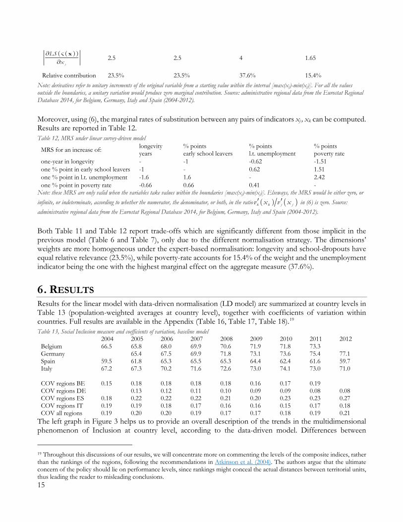
6. RESULTS Results for the linear model with data-driven normalisation (LD model) are summarized at country levels in Table 13 (population-weighted averages at country level), together with coefficients of variation within countries. Full results are available in the Appendix (Table 16, Table 17, Table 18).19 Table 13, Social Inclusion measure and coefficients of variation, baseline model
2004 2005 2006 2007 2008 2009 2010 2011 2012 Belgium 66.5 65.8 68.0 69.9 70.6 71.9 71.8 73.3 Germany 65.4 67.5 69.9 71.8 73.1 73.6 75.4 77.1 Spain 59.5 61.8 65.3 65.5 65.3 64.4 62.4 61.6 59.7 Italy 67.2 67.3 70.2 71.6 72.6 73.0 74.1 73.0 71.0 COV regions BE 0.15 0.18 0.18 0.18 0.18 0.16 0.17 0.19 COV regions DE 0.13 0.12 0.11 0.10 0.09 0.09 0.08 0.08 COV regions ES 0.18 0.22 0.22 0.22 0.21 0.20 0.23 0.23 0.27 COV regions IT 0.19 0.19 0.18 0.17 0.16 0.16 0.15 0.17 0.18 COV all regions 0.19 0.20 0.20 0.19 0.17 0.17 0.18 0.19 0.21
The left graph in Figure 3 helps us to provide an overall description of the trends in the multidimensional phenomenon of Inclusion at country level, according to the data-driven model. Differences between
19 Throughout this discussions of our results, we will concentrate more on commenting the levels of the composite indices, rather than the rankings of the regions, following the recommendations in Atkinson et al. (2004). The authors argue that the ultimate concern of the policy should lie on performance levels, since rankings might conceal the actual distances between territorial units, thus leading the reader to misleading conclusions. 15
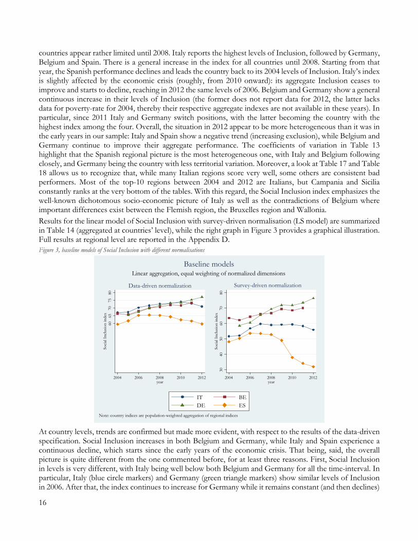
countries appear rather limited until 2008. Italy reports the highest levels of Inclusion, followed by Germany, Belgium and Spain. There is a general increase in the index for all countries until 2008. Starting from that year, the Spanish performance declines and leads the country back to its 2004 levels of Inclusion. Italy’s index is slightly affected by the economic crisis (roughly, from 2010 onward): its aggregate Inclusion ceases to improve and starts to decline, reaching in 2012 the same levels of 2006. Belgium and Germany show a general continuous increase in their levels of Inclusion (the former does not report data for 2012, the latter lacks data for poverty-rate for 2004, thereby their respective aggregate indexes are not available in these years). In particular, since 2011 Italy and Germany switch positions, with the latter becoming the country with the highest index among the four. Overall, the situation in 2012 appear to be more heterogeneous than it was in the early years in our sample: Italy and Spain show a negative trend (increasing exclusion), while Belgium and Germany continue to improve their aggregate performance. The coefficients of variation in Table 13 highlight that the Spanish regional picture is the most heterogeneous one, with Italy and Belgium following closely, and Germany being the country with less territorial variation. Moreover, a look at Table 17 and Table 18 allows us to recognize that, while many Italian regions score very well, some others are consistent bad performers. Most of the top-10 regions between 2004 and 2012 are Italians, but Campania and Sicilia constantly ranks at the very bottom of the tables. With this regard, the Social Inclusion index emphasizes the well-known dichotomous socio-economic picture of Italy as well as the contradictions of Belgium where important differences exist between the Flemish region, the Bruxelles region and Wallonia. Results for the linear model of Social Inclusion with survey-driven normalisation (LS model) are summarized in Table 14 (aggregated at countries’ level), while the right graph in Figure 3 provides a graphical illustration. Full results at regional level are reported in the Appendix D. Figure 3, baseline models of Social Inclusion with different normalisations
At country levels, trends are confirmed but made more evident, with respect to the results of the data-driven specification. Social Inclusion increases in both Belgium and Germany, while Italy and Spain experience a continuous decline, which starts since the early years of the economic crisis. That being, said, the overall picture is quite different from the one commented before, for at least three reasons. First, Social Inclusion in levels is very different, with Italy being well below both Belgium and Germany for all the time-interval. In particular, Italy (blue circle markers) and Germany (green triangle markers) show similar levels of Inclusion in 2006. After that, the index continues to increase for Germany while it remains constant (and then declines)
6065
7075
80So
cial
Incl
usio
n in
dex
2004 2006 2008 2010 2012year
Data-driven normalization
3040
5060
7080
Soci
al In
clus
ion
inde
x
2004 2006 2008 2010 2012year
Survey-driven normalization
Note: country indices are population-weighted aggregation of regional indices
Linear aggregation, equal weighting of normalized dimensionsBaseline models
IT BEDE ES
16
in Italy. Thus, there is a clear phenomenon of rank reversal between the two models: in terms of “desirability” (as defined by the expert-panel), the aggregated Italian picture is worse than the German one. A look at Table 20 and Table 21 highlights how German regions, together with Belgium’s Flanders, achieve more top-10 rankings than they were under the previous specification, especially after 2007. Second, Spain exhibits a decline in Social Inclusion (an increase in Social Exclusion) which is much more dramatic than it appeared before. The negative trend starts after 2006 but the drop in performance is substantial after 2008, leading to levels of Inclusion much lower in 2012 than they were in 2004. Again, we stress the fact that, albeit the negative trend for Spain was already visible from the baseline data-driven model, this picture conveys a much stronger need for intervention. Third, the heterogeneity within each country is much higher, as noticeable from the coefficients of variation in Table 14. Spain, Italy and Belgium still report the highest coefficients, but heterogeneities are rather constant in the latter country while they are increasing in Italy and especially in Spain. An opposite trend appears in Germany, where convergence of Social Inclusion between regions seems to occur. It is important to recall, at this point, that none of these differences are due to changes in the core parameters of the aggregation function (the β, or the weights wj), but rather to the new re-scaling characterization, which has now an explicit interpretation in terms of desirability. Table 14, Social Inclusion measure and coefficients of variation, expert-based normalisation
2004 2005 2006 2007 2008 2009 2010 2011 2012 Belgium 63.5 62.2 64.4 66.1 66.7 69.4 68.5 70.1 Germany 58.6 60.5 65.4 69.3 71.9 71.9 73.4 76.3 Spain 48.2 50.3 53.6 53.5 52.8 49.0 38.0 34.2 32.0 Italy 51.6 52.2 56.7 59.7 59.0 59.2 59.4 58.3 55.9 COV regions BE 0.37 0.43 0.43 0.42 0.43 0.34 0.39 0.39 COV regions DE 0.28 0.26 0.24 0.22 0.19 0.17 0.16 0.13 COV regions ES 0.25 0.26 0.27 0.28 0.23 0.31 0.46 0.50 0.50 COV regions IT 0.39 0.34 0.30 0.31 0.31 0.32 0.32 0.38 0.34 COV all regions 0.20 0.22 0.22 0.28 0.21 0.32 0.34
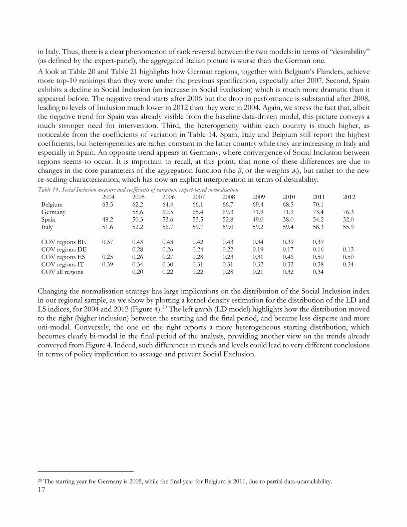
Changing the normalisation strategy has large implications on the distribution of the Social Inclusion index in our regional sample, as we show by plotting a kernel-density estimation for the distribution of the LD and LS indices, for 2004 and 2012 (Figure 4).20 The left graph (LD model) highlights how the distribution moved to the right (higher inclusion) between the starting and the final period, and became less disperse and more uni-modal. Conversely, the one on the right reports a more heterogeneous starting distribution, which becomes clearly bi-modal in the final period of the analysis, providing another view on the trends already conveyed from Figure 4. Indeed, such differences in trends and levels could lead to very different conclusions in terms of policy implication to assuage and prevent Social Exclusion.
20 The starting year for Germany is 2005, while the final year for Belgium is 2011, due to partial data-unavailability. 17
Figure 4, distributions of Inclusion Indices
Finally, in order to test whether the two specifications convey similar rankings, we perform a Kendall’s tau21 tests between the ranking of the data-driven model and the one coming from the survey-driven model, for each year. Results are reported in Table 15. Coefficients’ magnitude indicate that rakings’ correspondence is far from perfect, yet we can always reject (at 99%) the null-hypothesis of no correlation between the models’ rankings. Coefficients are lower than those found in similar analyses, as Carrino (2013). A reason for this is that the latter study was limited to Italian regional data, which presents a rather consolidated pattern of dominance between regions, so that the rankings are less affected by changes in model design. Table 15, Kendall’s τ correlation coefficients
2005 2006 2007 2008 2009 2010 2011 2012 Average Kendall’s τ 0.78 0.80 0.78 0.75 0.73 0.73 0.78 0.78 0.76
6.1 ON THE RANK-REVERSAL BETWEEN GERMANY AND ITALY Since 2004, Germany and Italy exhibit similar trends in early school-leaving, life expectancy at birth and poverty rate. Nevertheless, the levels of these variables are quite different: there are much more school-dropouts and poverty rates in Italy, which also presents substantially higher longevity. When it comes to long-term unemployment, the country-trends are crossing: Italy experienced a consistent decline in its labour market performance, while Germany saw a constant improvement (according to many observers, a consequence of the Hartz Reforms). Such trends are summarised in Figure 12 (Appendix D). Figure 5 and Figure 6 report the values of the four indicators normalised according to, respectively, the data-driven and the expert-based min-max functions. The dashed thick lines in both Figures denote the social exclusion indices obtained by simple averages. For both Germany and Italy, the normalised poverty-rate is quite flat according to both normalisations strategies. In the data-driven model for Italy (the left graph of Figure 5), the increase in normalised life-expectancy more than counterbalances, due to its substantially higher relative weight, the worsening conditions in the labour market, therefore allowing the overall measure to increase slightly. Almost no role is played by early school-leaving, which has very little variations. In Germany, all the dimensions improve, thus leading to a
21 The Kendall-τ test is a non parametric method that allows to measure the degree of correspondence between two rankings. In particular, the Kendall-τ b allows for the possibility of ties in the rankings. Command in STATA: ktau. A resulting test-value of zero would indicate that no correlation exist between the two rankings, while a value of 1 would indicate perfect correlation. Conversely, negative values (down to a minimum of -1) would indicate that rankings are inverted.
0
.01
.02
.03
Den
sity
20 40 60 80 100
Social Inclusion Index LDkernel = epanechnikov, bandwidth = 4.7235
LD: linear + data-driven normalization
.005
.01
.015
.02
Den
sity
20 40 60 80 100
Social Inclusion Index LSkernel = epanechnikov, bandwidth = 6.8764
LS: linear + survey-based normalization
Kernel density estimates for LD and LS indices' distribution
year 2004year 2012
18

regular increase in the composite measure, yet the Inclusion index is lower than for Italy, exactly because of the weight given to life expectancy. When the elicited benchmarks are implemented (Figure 6), life expectancy becomes the best performing dimension for Italy, while early school-leaving is heavily penalized. In Germany, both these normalised-attributes are much higher than under the data-driven model. Finally, although being rather small in 2004, the spread between the countries’ long-term unemployment normalised-rates becomes much more evident. Given the reduced relative weight given to longevity in the expert-based model, and the higher one given to long-term unemployment, the German index is (1) higher than Italy, while it was lower in the previous specification; and (2) increasing at a higher rate. Figure 5, data-drivem normalised time trends in Germany and Italy
Figure 6, survey-driven normalised time trends in Germany and Italy
5060708090
Nor
mal
ized
val
ue
2004 2006 2008 2010 2012year
Regional aggregation with population weightsItaly
20
40
60
80
100
Nor
mal
ized
val
ue
2004 2006 2008 2010 2012year
Regional aggregation with population weightsGermany
Normalization benchmarks: poverty rate (5.2%; 48.9%), long-term unemployment (0.5%; 18.2%), early school-leaving (5.4%; 54.2%), life expectancy (77.5; 84.2)
Time trend of data-driven normalized indicators
Poverty rate Long-term unemploymentEarly school-leaving Life expectancy at birthSimple average
2040
6080
100
Nor
mal
ized
valu
e
2004 2006 2008 2010 2012year
Regional aggregation with population weightsItaly
4060
8010
0N
orm
aliz
ed v
alue
2004 2006 2008 2010 2012year
Regional aggregation with population weightsGermany
Normalization benchmarks: poverty rate (5%; 20%), long-term unemployment (3%; 9%), early school-leaving (10%; 20%), life expectancy (73; 83)
Time trend of survey-based normalized indicators
Poverty rate Long-term unemploymentEarly school-leaving Life expectancy at birthSimple average
19
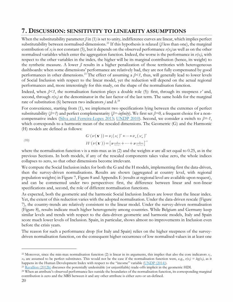
7. DISCUSSION: SENSITIVITY TO LINEARITY ASSUMPTIONS When the substitutability parameter β in (1) is set to unity, indifference curves are linear, which implies perfect substitutability between normalised-dimensions.22 If this hypothesis is relaxed (β less than one), the marginal contribution of xj is not constant (5), but it depends on the observed performance v(xj) as well as on the other normalised variables which enter the aggregation function. Indeed, the worse is the performance in v(xj), with respect to the other variables in the index, the higher will be its marginal contribution (hence, its weight) to the synthetic measure. A lower β results in a higher penalization of those territories with heterogeneous dashboards: when some dimensions’ performance are relatively bad, they are not fully compensated by good performances in other dimensions.23 The effect of assuming a β<1, thus, will generally lead to lower levels of Social Inclusion with respect to the linear model, yet the reduction will depend on the actual regional performances and, more interestingly for this study, on the shape of the normalisation function. Indeed, when β<1, the normalisation function plays a double role (5): first, through its steepness v’ and, second, through v(xj) at the denominator in the last factor of the last term. The same holds for the marginal rate of substitution (6) between two indicators j and h.24 For convenience, starting from (1), we implement two specifications lying between the extremes of perfect substitutability (β=1) and perfect complementarity (β=-infinity). We first set β=0, a frequent choice for a non-compensative index (Silva and Ferreira-Lopes 2013; UNDP 2010). Second, we consider a switch to β=-1, which corresponds to a harmonic mean of the rescaled dimensions. The Geometric (G) and the Harmonic (H) models are defined as follows:
(10)
< >1 1
1 1
11 1i i
m m
w wi i i im m
i ixx
G x x
H w w OO
O O O
O �
� � �
� � �
"
"
x
x
where the normalisation function ν is a min-max as in (2) and the weights w are all set equal to 0.25, as in the previous Sections. In both models, if any of the rescaled components takes value zero, the whole indices collapses to zero, so that other dimensions become irrelevant. We compute the Social Inclusion index for both the G and the H models, implementing first the data-driven, then the survey-driven normalisations. Results are shown (aggregated at country level, with regional population weights) in Figure 7, Figure 8 and Appendix E (results at regional level are available upon request), and can be commented under two perspectives: first, the difference between linear and non-linear specifications and, second, the role of different normalisation functions. As expected, both the geometric and the harmonic Social Inclusion Indices are lower than the linear index. Yet, the extent of this reduction varies with the adopted normalisation. Under the data-driven rescale (Figure 7), the country-trends are relatively consistent to the linear model. Under the survey-driven normalisation (Figure 8), results indicate much higher heterogeneity among countries. While Belgium and Germany keep similar levels and trends with respect to the data-driven geometric and harmonic models, Italy and Spain score much lower levels of Inclusion. Spain, in particular, shows almost no improvements in Inclusion even before the crisis years. The reason for such a performance drop (for Italy and Spain) relies on the higher steepness of the survey-driven normalisation function, on the consequent higher occurrence of low normalised-values in at least one
22 Moreover, since the min-max normalisation function (2) is linear in its arguments, this implies that also the core indicators xj , xk are assumed to be perfect substitutes. This would not be the case if the normalisation function were, e.g., v(xj) = log(xj), as it happens in the Human Development Index with respect to the “income” variable (UNDP (2014)). 23 Ravallion (2012b) discusses the potentially undesirable (or unjustifiable) trade-offs implicit in the geometric HDI. 24 When an attribute’s observed performance lies outside the boundaries of the normalisation function, its corresponding marginal contribution is zero and the MRS between it and any other attribute is either zero or un-defined. 20

dimension, and in the weights implied by the expert-based rescaling, which penalise Italy and Spain, as already discussed in Section 6.1. Figure 7, geometric and harmonic models, data-driven
Figure 8, geometric and harmonic models, survey-driven
Changing the normalisation strategy can sensibly alter the levels of the aggregate measure, as well as its rankings. Figure 9 summarizes the rankings obtained for each administrative region after computing the average indices between 2004 and 2012 under the linear, geometric and harmonic framework, and for both the data-driven and the survey-driven normalisation. Territories are sorted by their ranking in the linear data-driven model. Furthermore, data-driven rankings are characterized by “x” symbols, survey-driven rankings by “circles”. Both the categories appear in markers of different size, depending on the degree of substitutability implied in the models. The graph highlights rankings’ heterogeneity. Focusing just on the “big X” and “big circle” (the linear specifications), it is visible that several regions are “penalized” by the data-driven normalisation (i.e., the “x” lies below the “circle”), while the opposite occurs when the “x” lies above the “circle”. More importantly, changing the substitutability degree within the data-driven framework (i.e., when switching from the big “x” to the smaller ones) produces far less variation in the rankings than it does changing the models within the
5560657075
Socia
l Inc
lusio
n in
dex
2004 2006 2008 2010 2012year
European countries (regional pop. weighted)Geometric model with data-driven normalization
40
50
60
70
80
Socia
l Inc
lusio
n in
dex
2004 2006 2008 2010 2012year
European countries (regional pop. weighted)Armonic model with data-driven normalization
IT BEDE ES
020
4060
80So
cial I
nclu
sion
inde
x
2004 2006 2008 2010 2012year
European countries (regional pop. weighted)Geometric model with survey-driven normalization
020
4060
80So
cial I
nclu
sion
inde
x
2004 2006 2008 2010 2012year
European countries (regional pop. weighted)Armonic model with survey-driven normalization
IT BEDE ES
21
survey-driven framework (the distance between the big “circles” and the smaller ones).25 Note also that, in many occasions, the switch to complementarity (either geometric or harmonic) causes rankings to change in opposite directions, depending on which normalisation is adopted (e.g., the 6th, the 12th and 13th observations from the left). Figure 9, rankings' sensitivity
Finally, heterogeneities are not randomly occurring across regions. There are visible groups of “highly ranked” and “badly ranked” territories, which do not move much, regardless of the aggregation and normalisation choices. The former are concentrated in the Northeast and Centre of Italy, the Flemish Belgian region, the Baden-Württemberg and Bayern in Germany, the País Vasco and Comunidad Foral de Navarra in Spain. Among the latter we find most of the Southern Italian and Spanish regions (including the islands), as well as the Belgian Bruxelles region of Belgium.
8. CONCLUSION The unavoidable subjectivity of composite measures of Well-being are cause of controversies in this field of economic analysis. In this paper, we argued that the lack of transparency on methodological choices can turn out more troublesome than subjectivity per se, and we particularly focus on the choices of the normalisation function. In the context of building a synthetic Index of Social Inclusion for 58 administrative regions in
25 Table 26 reports average Kendall’s τ coefficients between the rankings generated by the data-driven and the survey-driven models computed so far. All Kendall’s τ coefficients allow to significantly reject (at 99%) the null hypothesis of independence in rankings. Yet, the coefficients corresponding to comparisons involving any geometric or harmonic model are lower than those involving linear-models-only: changing both the aggregation model and the normalisation function can indeed lead to substantially different rankings. Furthermore, changing the aggregation model within the data-driven framework (reading the table column-wise, e.g. from top to bottom, regardless of the column) produces far less variation in the Kendall’s τ coefficients than it does changing model within the survey-driven framework (reading the table row-wise, from left to right, regardless of the row), confirming the results in Carrino (2013) (in Italian).
111
2131
4151
61ra
nkin
g
ITD
1 E
S22
ITD
5 IT
D3
ITE3
DE1
ITE1
ITE2
ITD
4 IT
C4 E
S21
BE2
DE2
ITC3
ITC2
ITC1
ES3
0 D
E7 IT
E4 IT
F1 E
S24
ES1
3 D
EB D
E60
DEF
0 D
E9 E
S41
DEA
ES1
2 IT
F2 E
S51
ES2
3 E
S11
DEG
0 D
ED D
EC0
DE4
0 IT
F5 IT
G2
ES5
3 D
E50
DE3
0 E
S52
ITF4
BE3
ITF6
DE8
0 E
S42
DEE
0 E
S62
BE1
0 E
S70
ES4
3 IT
F3 E
S61
ITG
1 E
S64
ES6
3
Data-driven linear Survey-driven linearData-driven geometric Survey-driven geometricData-driven harmonic Survey-driven harmonic
Administrative regions in Europe, multiple models, ranking of average indices 2004-2012Rankings' sensitivity to normalization
22

Europe between 2004 and 2012, we showed the consequences of adopting different normalisation methods while keeping the aggregation model unchanged, with equal weights on the normalised dimensions. To the extent to which rescaling is a requirement for composite measures, the actual aggregation involves the transformed variables, rather than the observed performances. There is an unavoidable and intrinsic difference between the interpretation of original and normalised performances, and yet social researchers are ultimately interested in the contribution of the original variables to the aggregate index. The rescaled unit of measurement (e.g., between zero and one-hundred) can be interpreted as a sort of degree of fulfilment of some criterion. Whether this criterion should be purely statistical (e.g., being far or close to the observed minimum or maximum observed achievements), or whether it should encompass some informed value judgements related to the topic at hand (as in the expert elicitation or in the adoption of policy benchmarks), relies on the researcher’s choice. In the former case, the agnostic choice of “letting the data talk”, the standard properties as strong non-satiation and continuity of the normalisation function are guaranteed, yet dimensions’ trade-offs might be hard to interpret in economic terms and debatable from a social desirability perspective. Therefore, the resulting aggregate measure would be characterized as a tool for mainly “positive” analysis. In the latter case, conversely, the normalisation function may become weakly monotonic, when the elicited constraints are binding for some observed variable. Moreover, the elicitation method suffers from the arbitrariness embedded in any survey exercise (choice of the population, bias in the framing of questions). Dimensions trade-offs reflect the preferences of an actual group of experts, are independent from the data-selection, and allow to characterize the final measure with a “normative” connotation. The main result of our analysis is that neither method is neutral. Data-driven normalisation softens the aftermaths of the recent economic crisis, by putting a consistent weight on the longevity variable. Conversely, the survey-driven normalisation emphasizes the worsening trends in long-term unemployment and the relevance of early school-leaving. As a result, numerous rank-reversals occur between regions when switching the normalisation methods. Finally, the normalisation choice has even stronger consequences when the allowed substitutability between dimensions is lower (e.g., in a geometric or harmonic aggregation).
BIBLIOGRAPHY Anand, S., & Sen, A. (1994). Human development index: methodology and measurement. Human Development Report Office
(HDRO), United Nations Development Programme (UNDP). Atkinson, A. B., Cantillon, B., Marlier, E., & Nolan, B. (2002). Social Indicators: The EU and Social Inclusion: The EU and Social Inclusion:
Oxford University Press. Atkinson, A. B., Marlier, E., & Nolan, B. (2004). Indicators and targets for social inclusion in the European Union. JCMS: Journal
of Common Market Studies, 42(1), 47-75. Blackorby, C., & Donaldson, D. (1982). Ratio-scale and translation-scale full interpersonal comparability without domain
restrictions: Admissible social-evaluation functions. International Economic Review, 249-268. Boarini, R., & D'Ercole, M. M. (2013). Going beyond GDP: An OECD Perspective*. Fiscal Studies, 34(3), 289-314,
doi:10.1111/j.1475-5890.2013.12007.x. Bourguignon, F., & Chakravarty, S. R. (2003). The measurement of multidimensional poverty. The Journal of Economic Inequality,
1(1), 25-49. Carrino, L. (2013). L’esclusione sociale in Italia: approcci alternativi per un’indagine regionale. Analisi e strumenti di politica sociale, 45. Cherchye, L., Knox Lovell, C. A., Moesen, W., & Van Puyenbroeck, T. (2007). One market, one number? A composite indicator
assessment of EU internal market dynamics. European Economic Review, 51(3), 749-779, doi:http://dx.doi.org/10.1016/j.euroecorev.2006.03.011.
Chowdhury, S., & Squire, L. (2006). Setting weights for aggregate indices: An application to the commitment to development index and human development index. Journal of Development Studies, 42(5), 761-771.
Decancq, K., & Lugo, M. A. (2008). Setting weights in multidimensional indices of well-being. Decancq, K., & Lugo, M. A. (2009). Measuring inequality of well-being with a correlation-sensitive multidimensional Gini index.
University of Oxford Department of Economics Discussion Paper Series, 459.
23
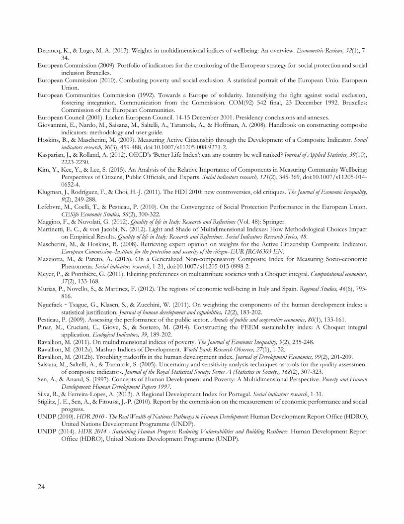
Decancq, K., & Lugo, M. A. (2013). Weights in multidimensional indices of wellbeing: An overview. Econometric Reviews, 32(1), 7-34.
European Commission (2009). Portfolio of indicators for the monitoring of the European strategy for social protection and social inclusion Bruxelles.
European Commission (2010). Combating poverty and social exclusion. A statistical portrait of the European Unio. European Union.
European Communities Commission (1992). Towards a Europe of solidarity. Intensifying the fight against social exclusion, fostering integration. Communication from the Commission. COM(92) 542 final, 23 December 1992. Bruxelles: Commission of the European Communities.
European Council (2001). Laeken European Council. 14-15 December 2001. Presidency conclusions and annexes. Giovannini, E., Nardo, M., Saisana, M., Saltelli, A., Tarantola, A., & Hoffman, A. (2008). Handbook on constructing composite
indicators: methodology and user guide. Hoskins, B., & Mascherini, M. (2009). Measuring Active Citizenship through the Development of a Composite Indicator. Social
indicators research, 90(3), 459-488, doi:10.1007/s11205-008-9271-2. Kasparian, J., & Rolland, A. (2012). OECD's ‘Better Life Index’: can any country be well ranked? Journal of Applied Statistics, 39(10),
2223-2230. Kim, Y., Kee, Y., & Lee, S. (2015). An Analysis of the Relative Importance of Components in Measuring Community Wellbeing:
Perspectives of Citizens, Public Officials, and Experts. Social indicators research, 121(2), 345-369, doi:10.1007/s11205-014-0652-4.
Klugman, J., Rodríguez, F., & Choi, H.-J. (2011). The HDI 2010: new controversies, old critiques. The Journal of Economic Inequality, 9(2), 249-288.
Lefebvre, M., Coelli, T., & Pestieau, P. (2010). On the Convergence of Social Protection Performance in the European Union. CESifo Economic Studies, 56(2), 300-322.
Maggino, F., & Nuvolati, G. (2012). Quality of life in Italy: Research and Reflections (Vol. 48): Springer. Martinetti, E. C., & von Jacobi, N. (2012). Light and Shade of Multidimensional Indexes: How Methodological Choices Impact
on Empirical Results. Quality of life in Italy: Research and Reflections. Social Indicators Research Series, 48. Mascherini, M., & Hoskins, B. (2008). Retrieving expert opinion on weights for the Active Citizenship Composite Indicator.
European Commission–Institute for the protection and security of the citizen–EUR JRC46303 EN. Mazziotta, M., & Pareto, A. (2015). On a Generalized Non-compensatory Composite Index for Measuring Socio-economic
Phenomena. Social indicators research, 1-21, doi:10.1007/s11205-015-0998-2. Meyer, P., & Ponthière, G. (2011). Eliciting preferences on multiattribute societies with a Choquet integral. Computational economics,
37(2), 133-168. Murias, P., Novello, S., & Martinez, F. (2012). The regions of economic well-being in Italy and Spain. Regional Studies, 46(6), 793-
816. Nguefack‐Tsague, G., Klasen, S., & Zucchini, W. (2011). On weighting the components of the human development index: a
statistical justification. Journal of human development and capabilities, 12(2), 183-202. Pestieau, P. (2009). Assessing the performance of the public sector. Annals of public and cooperative economics, 80(1), 133-161. Pinar, M., Cruciani, C., Giove, S., & Sostero, M. (2014). Constructing the FEEM sustainability index: A Choquet integral
application. Ecological Indicators, 39, 189-202. Ravallion, M. (2011). On multidimensional indices of poverty. The Journal of Economic Inequality, 9(2), 235-248. Ravallion, M. (2012a). Mashup Indices of Development. World Bank Research Observer, 27(1), 1-32. Ravallion, M. (2012b). Troubling tradeoffs in the human development index. Journal of Development Economics, 99(2), 201-209. Saisana, M., Saltelli, A., & Tarantola, S. (2005). Uncertainty and sensitivity analysis techniques as tools for the quality assessment
of composite indicators. Journal of the Royal Statistical Society: Series A (Statistics in Society), 168(2), 307-323. Sen, A., & Anand, S. (1997). Concepts of Human Development and Poverty: A Multidimensional Perspective. Poverty and Human
Development: Human Development Papers 1997. Silva, R., & Ferreira-Lopes, A. (2013). A Regional Development Index for Portugal. Social indicators research, 1-31. Stiglitz, J. E., Sen, A., & Fitoussi, J.-P. (2010). Report by the commission on the measurement of economic performance and social
progress. UNDP (2010). HDR 2010 - The Real Wealth of Nations: Pathways to Human Development: Human Development Report Office (HDRO),
United Nations Development Programme (UNDP). UNDP (2014). HDR 2014 - Sustaining Human Progress: Reducing Vulnerabilities and Building Resilience: Human Development Report
Office (HDRO), United Nations Development Programme (UNDP).
24
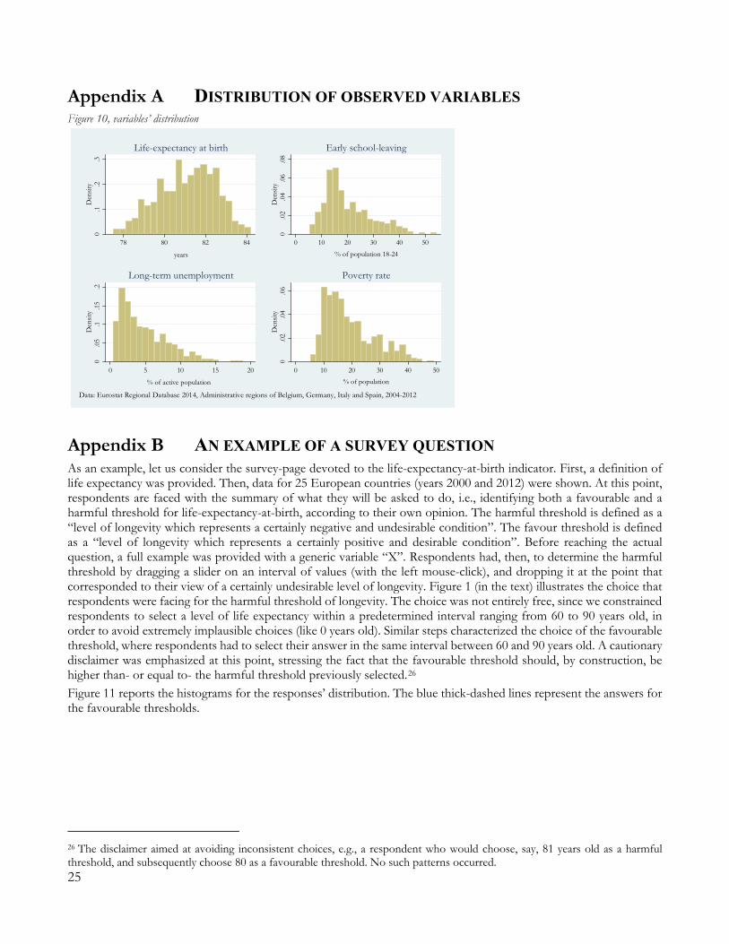
DISTRIBUTION OF OBSERVED VARIABLES Figure 10, variables’ distribution
AN EXAMPLE OF A SURVEY QUESTION As an example, let us consider the survey-page devoted to the life-expectancy-at-birth indicator. First, a definition of life expectancy was provided. Then, data for 25 European countries (years 2000 and 2012) were shown. At this point, respondents are faced with the summary of what they will be asked to do, i.e., identifying both a favourable and a harmful threshold for life-expectancy-at-birth, according to their own opinion. The harmful threshold is defined as a “level of longevity which represents a certainly negative and undesirable condition”. The favour threshold is defined as a “level of longevity which represents a certainly positive and desirable condition”. Before reaching the actual question, a full example was provided with a generic variable “X”. Respondents had, then, to determine the harmful threshold by dragging a slider on an interval of values (with the left mouse-click), and dropping it at the point that corresponded to their view of a certainly undesirable level of longevity. Figure 1 (in the text) illustrates the choice that respondents were facing for the harmful threshold of longevity. The choice was not entirely free, since we constrained respondents to select a level of life expectancy within a predetermined interval ranging from 60 to 90 years old, in order to avoid extremely implausible choices (like 0 years old). Similar steps characterized the choice of the favourable threshold, where respondents had to select their answer in the same interval between 60 and 90 years old. A cautionary disclaimer was emphasized at this point, stressing the fact that the favourable threshold should, by construction, be higher than- or equal to- the harmful threshold previously selected.26 Figure 11 reports the histograms for the responses’ distribution. The blue thick-dashed lines represent the answers for the favourable thresholds.
26 The disclaimer aimed at avoiding inconsistent choices, e.g., a respondent who would choose, say, 81 years old as a harmful threshold, and subsequently choose 80 as a favourable threshold. No such patterns occurred.
0.1
.2.3
Den
sity
78 80 82 84
years
Life-expectancy at birth
0.0
2.0
4.0
6.0
8D
ensit
y
0 10 20 30 40 50
% of population 18-24
Early school-leaving
0.0
5.1
.15
.2D
ensit
y
0 5 10 15 20
% of active population
Long-term unemployment0
.02
.04
.06
Den
sity
0 10 20 30 40 50% of population
Poverty rate
Data: Eurostat Regional Database 2014, Administrative regions of Belgium, Germany, Italy and Spain, 2004-2012
25
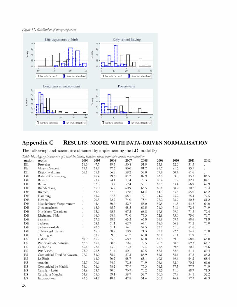
Figure 11, distribution of survey responses
RESULTS: MODEL WITH DATA-DRIVEN NORMALISATION The following coefficients are obtained by implementing the LD model (8) Table 16, Aggregate measure of Social Inclusion, baseline model with data-driven normalisation
nation region 2004 2005 2006 2007 2008 2009 2010 2011 2012 BE Bruxelles 51.3 47.7 49.5 50.8 51.8 55.1 52.6 51.3 . BE Vlaams Gewest 75.1 75.2 77.6 80.0 81.2 81.7 81.6 83.9 . BE Région wallonne 56.1 55.1 56.8 58.2 58.0 59.9 60.4 61.6 . DE Baden-Württemberg . 76.4 79.6 81.2 82.9 83.0 83.0 85.3 86.5 DE Bayern . 73.4 74.4 77.4 79.3 80.4 81.2 82.1 84.1 DE Berlin . 52.3 53.7 59.4 59.1 62.9 63.4 66.9 67.9 DE Brandenburg . 55.0 56.9 60.9 65.5 66.8 68.7 70.2 70.4 DE Bremen . 51.3 57.6 59.8 61.4 64.3 65.5 65.0 68.2 DE Hamburg . 63.2 67.3 68.1 72.7 74.2 75.2 75.4 77.5 DE Hessen . 70.3 72.7 74.0 75.4 77.2 78.9 80.5 81.2 DE Mecklenburg-Vorpommern . 45.4 50.6 52.7 58.0 59.5 61.5 63.8 64.0 DE Niedersachsen . 63.9 65.7 68.5 69.5 71.0 71.6 72.6 74.9 DE Nordrhein-Westfalen . 63.6 65.3 67.2 68.8 69.8 69.6 71.5 72.4 DE Rheinland-Pfalz . 66.0 68.9 71.0 73.3 72.8 73.0 75.0 76.7 DE Saarland . 57.3 58.5 65.2 65.9 66.8 69.7 68.6 71.9 DE Sachsen . 58.1 61.1 62.9 67.1 68.0 66.2 71.2 73.0 DE Sachsen-Anhalt . 47.5 51.1 54.1 54.5 57.7 61.0 61.6 DE Schleswig-Holstein . 66.3 68.7 70.9 71.3 72.8 72.6 74.8 75.8 DE Thüringen . 58.7 59.0 61.2 65.8 68.8 71.1 71.9 73.1 ES Galicia 60.9 65.7 65.8 68.3 68.8 67.9 69.0 68.0 66.0 ES Principado de Asturias 62.5 65.4 68.5 70.6 72.5 70.5 68.5 69.3 64.7 ES Cantabria 66.4 72.4 73.6 73.3 77.4 75.5 69.5 70.8 74.6 ES País Vasco 75.9 78.5 81.4 80.1 82.5 82.1 82.6 81.1 80.4 ES Comunidad Foral de Navarra 77.7 81.0 85.7 87.2 85.9 86.1 88.4 87.5 85.2 ES La Rioja 64.9 70.2 68.7 65.1 69.1 69.4 64.2 68.4 ES Aragón 72.7 70.6 74.7 72.5 74.9 76.6 72.0 70.2 69.6 ES Comunidad de Madrid 74.6 74.6 78.2 77.9 77.3 76.5 77.5 77.7 74.9 ES Castilla y León 64.8 65.7 70.0 70.9 70.2 71.5 71.0 68.7 71.3 ES Castilla-la Mancha 54.9 55.3 59.1 58.7 58.7 60.0 57.9 54.1 52.2 ES Extremadura 42.5 44.2 48.7 47.8 51.4 50.9 46.4 52.3 42.3
0.0
5.1
.15
.2
Den
sity
60 70 80 90
harmful threshold favorable threshold
Life-expectancy at birth
0.0
5.1
.15
.2
Den
sity
0 10 20 30 40
harmful threshold favorable threshold
Early school-leaving
0.0
5.1
.15
.2.2
5
Den
sity
0 10 20 30 40
harmful threshold favorable threshold
Long-term unemployment
0.0
5.1
.15
.2
Den
sity
0 10 20 30 40
harmful threshold favorable threshold
Poverty-rate
26
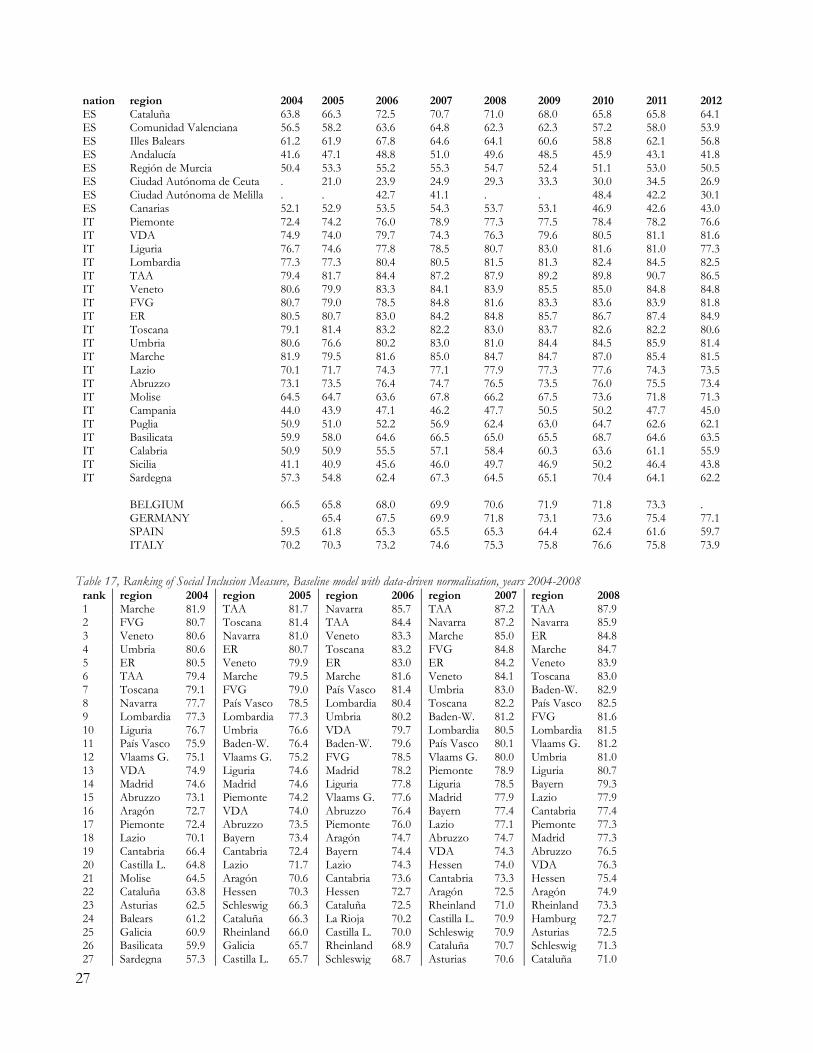
nation region 2004 2005 2006 2007 2008 2009 2010 2011 2012 ES Cataluña 63.8 66.3 72.5 70.7 71.0 68.0 65.8 65.8 64.1 ES Comunidad Valenciana 56.5 58.2 63.6 64.8 62.3 62.3 57.2 58.0 53.9 ES Illes Balears 61.2 61.9 67.8 64.6 64.1 60.6 58.8 62.1 56.8 ES Andalucía 41.6 47.1 48.8 51.0 49.6 48.5 45.9 43.1 41.8 ES Región de Murcia 50.4 53.3 55.2 55.3 54.7 52.4 51.1 53.0 50.5 ES Ciudad Autónoma de Ceuta . 21.0 23.9 24.9 29.3 33.3 30.0 34.5 26.9 ES Ciudad Autónoma de Melilla . . 42.7 41.1 . . 48.4 42.2 30.1 ES Canarias 52.1 52.9 53.5 54.3 53.7 53.1 46.9 42.6 43.0 IT Piemonte 72.4 74.2 76.0 78.9 77.3 77.5 78.4 78.2 76.6 IT VDA 74.9 74.0 79.7 74.3 76.3 79.6 80.5 81.1 81.6 IT Liguria 76.7 74.6 77.8 78.5 80.7 83.0 81.6 81.0 77.3 IT Lombardia 77.3 77.3 80.4 80.5 81.5 81.3 82.4 84.5 82.5 IT TAA 79.4 81.7 84.4 87.2 87.9 89.2 89.8 90.7 86.5 IT Veneto 80.6 79.9 83.3 84.1 83.9 85.5 85.0 84.8 84.8 IT FVG 80.7 79.0 78.5 84.8 81.6 83.3 83.6 83.9 81.8 IT ER 80.5 80.7 83.0 84.2 84.8 85.7 86.7 87.4 84.9 IT Toscana 79.1 81.4 83.2 82.2 83.0 83.7 82.6 82.2 80.6 IT Umbria 80.6 76.6 80.2 83.0 81.0 84.4 84.5 85.9 81.4 IT Marche 81.9 79.5 81.6 85.0 84.7 84.7 87.0 85.4 81.5 IT Lazio 70.1 71.7 74.3 77.1 77.9 77.3 77.6 74.3 73.5 IT Abruzzo 73.1 73.5 76.4 74.7 76.5 73.5 76.0 75.5 73.4 IT Molise 64.5 64.7 63.6 67.8 66.2 67.5 73.6 71.8 71.3 IT Campania 44.0 43.9 47.1 46.2 47.7 50.5 50.2 47.7 45.0 IT Puglia 50.9 51.0 52.2 56.9 62.4 63.0 64.7 62.6 62.1 IT Basilicata 59.9 58.0 64.6 66.5 65.0 65.5 68.7 64.6 63.5 IT Calabria 50.9 50.9 55.5 57.1 58.4 60.3 63.6 61.1 55.9 IT Sicilia 41.1 40.9 45.6 46.0 49.7 46.9 50.2 46.4 43.8 IT Sardegna 57.3 54.8 62.4 67.3 64.5 65.1 70.4 64.1 62.2 BELGIUM 66.5 65.8 68.0 69.9 70.6 71.9 71.8 73.3 . GERMANY . 65.4 67.5 69.9 71.8 73.1 73.6 75.4 77.1 SPAIN 59.5 61.8 65.3 65.5 65.3 64.4 62.4 61.6 59.7 ITALY 70.2 70.3 73.2 74.6 75.3 75.8 76.6 75.8 73.9
Table 17, Ranking of Social Inclusion Measure, Baseline model with data-driven normalisation, years 2004-2008
rank region 2004 region 2005 region 2006 region 2007 region 2008 1 Marche 81.9 TAA 81.7 Navarra 85.7 TAA 87.2 TAA 87.9 2 FVG 80.7 Toscana 81.4 TAA 84.4 Navarra 87.2 Navarra 85.9 3 Veneto 80.6 Navarra 81.0 Veneto 83.3 Marche 85.0 ER 84.8 4 Umbria 80.6 ER 80.7 Toscana 83.2 FVG 84.8 Marche 84.7 5 ER 80.5 Veneto 79.9 ER 83.0 ER 84.2 Veneto 83.9 6 TAA 79.4 Marche 79.5 Marche 81.6 Veneto 84.1 Toscana 83.0 7 Toscana 79.1 FVG 79.0 País Vasco 81.4 Umbria 83.0 Baden-W. 82.9 8 Navarra 77.7 País Vasco 78.5 Lombardia 80.4 Toscana 82.2 País Vasco 82.5 9 Lombardia 77.3 Lombardia 77.3 Umbria 80.2 Baden-W. 81.2 FVG 81.6 10 Liguria 76.7 Umbria 76.6 VDA 79.7 Lombardia 80.5 Lombardia 81.5 11 País Vasco 75.9 Baden-W. 76.4 Baden-W. 79.6 País Vasco 80.1 Vlaams G. 81.2 12 Vlaams G. 75.1 Vlaams G. 75.2 FVG 78.5 Vlaams G. 80.0 Umbria 81.0 13 VDA 74.9 Liguria 74.6 Madrid 78.2 Piemonte 78.9 Liguria 80.7 14 Madrid 74.6 Madrid 74.6 Liguria 77.8 Liguria 78.5 Bayern 79.3 15 Abruzzo 73.1 Piemonte 74.2 Vlaams G. 77.6 Madrid 77.9 Lazio 77.9 16 Aragón 72.7 VDA 74.0 Abruzzo 76.4 Bayern 77.4 Cantabria 77.4 17 Piemonte 72.4 Abruzzo 73.5 Piemonte 76.0 Lazio 77.1 Piemonte 77.3 18 Lazio 70.1 Bayern 73.4 Aragón 74.7 Abruzzo 74.7 Madrid 77.3 19 Cantabria 66.4 Cantabria 72.4 Bayern 74.4 VDA 74.3 Abruzzo 76.5 20 Castilla L. 64.8 Lazio 71.7 Lazio 74.3 Hessen 74.0 VDA 76.3 21 Molise 64.5 Aragón 70.6 Cantabria 73.6 Cantabria 73.3 Hessen 75.4 22 Cataluña 63.8 Hessen 70.3 Hessen 72.7 Aragón 72.5 Aragón 74.9 23 Asturias 62.5 Schleswig 66.3 Cataluña 72.5 Rheinland 71.0 Rheinland 73.3 24 Balears 61.2 Cataluña 66.3 La Rioja 70.2 Castilla L. 70.9 Hamburg 72.7 25 Galicia 60.9 Rheinland 66.0 Castilla L. 70.0 Schleswig 70.9 Asturias 72.5 26 Basilicata 59.9 Galicia 65.7 Rheinland 68.9 Cataluña 70.7 Schleswig 71.3 27 Sardegna 57.3 Castilla L. 65.7 Schleswig 68.7 Asturias 70.6 Cataluña 71.0
27
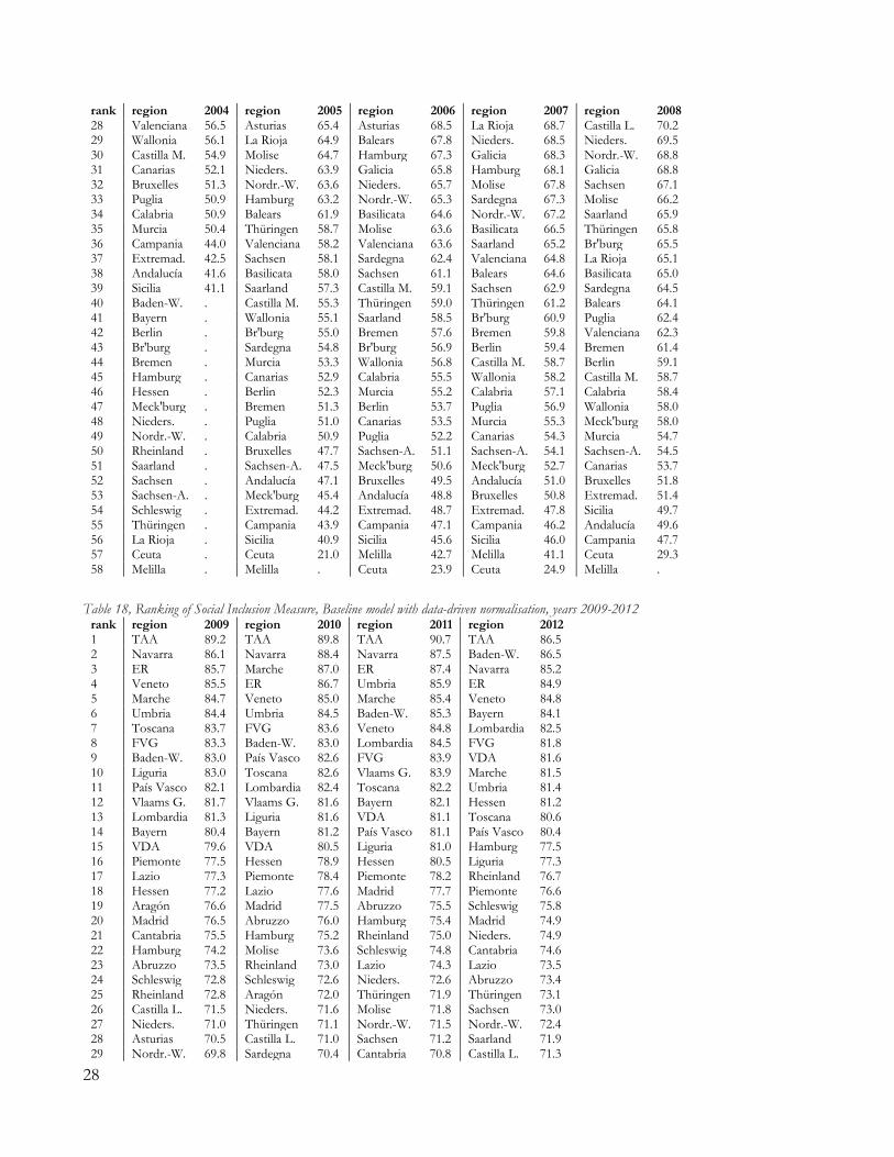
rank region 2004 region 2005 region 2006 region 2007 region 2008 28 Valenciana 56.5 Asturias 65.4 Asturias 68.5 La Rioja 68.7 Castilla L. 70.2 29 Wallonia 56.1 La Rioja 64.9 Balears 67.8 Nieders. 68.5 Nieders. 69.5 30 Castilla M. 54.9 Molise 64.7 Hamburg 67.3 Galicia 68.3 Nordr.-W. 68.8 31 Canarias 52.1 Nieders. 63.9 Galicia 65.8 Hamburg 68.1 Galicia 68.8 32 Bruxelles 51.3 Nordr.-W. 63.6 Nieders. 65.7 Molise 67.8 Sachsen 67.1 33 Puglia 50.9 Hamburg 63.2 Nordr.-W. 65.3 Sardegna 67.3 Molise 66.2 34 Calabria 50.9 Balears 61.9 Basilicata 64.6 Nordr.-W. 67.2 Saarland 65.9 35 Murcia 50.4 Thüringen 58.7 Molise 63.6 Basilicata 66.5 Thüringen 65.8 36 Campania 44.0 Valenciana 58.2 Valenciana 63.6 Saarland 65.2 Br'burg 65.5 37 Extremad. 42.5 Sachsen 58.1 Sardegna 62.4 Valenciana 64.8 La Rioja 65.1 38 Andalucía 41.6 Basilicata 58.0 Sachsen 61.1 Balears 64.6 Basilicata 65.0 39 Sicilia 41.1 Saarland 57.3 Castilla M. 59.1 Sachsen 62.9 Sardegna 64.5 40 Baden-W. . Castilla M. 55.3 Thüringen 59.0 Thüringen 61.2 Balears 64.1 41 Bayern . Wallonia 55.1 Saarland 58.5 Br'burg 60.9 Puglia 62.4 42 Berlin . Br'burg 55.0 Bremen 57.6 Bremen 59.8 Valenciana 62.3 43 Br'burg . Sardegna 54.8 Br'burg 56.9 Berlin 59.4 Bremen 61.4 44 Bremen . Murcia 53.3 Wallonia 56.8 Castilla M. 58.7 Berlin 59.1 45 Hamburg . Canarias 52.9 Calabria 55.5 Wallonia 58.2 Castilla M. 58.7 46 Hessen . Berlin 52.3 Murcia 55.2 Calabria 57.1 Calabria 58.4 47 Meck'burg . Bremen 51.3 Berlin 53.7 Puglia 56.9 Wallonia 58.0 48 Nieders. . Puglia 51.0 Canarias 53.5 Murcia 55.3 Meck'burg 58.0 49 Nordr.-W. . Calabria 50.9 Puglia 52.2 Canarias 54.3 Murcia 54.7 50 Rheinland . Bruxelles 47.7 Sachsen-A. 51.1 Sachsen-A. 54.1 Sachsen-A. 54.5 51 Saarland . Sachsen-A. 47.5 Meck'burg 50.6 Meck'burg 52.7 Canarias 53.7 52 Sachsen . Andalucía 47.1 Bruxelles 49.5 Andalucía 51.0 Bruxelles 51.8 53 Sachsen-A. . Meck'burg 45.4 Andalucía 48.8 Bruxelles 50.8 Extremad. 51.4 54 Schleswig . Extremad. 44.2 Extremad. 48.7 Extremad. 47.8 Sicilia 49.7 55 Thüringen . Campania 43.9 Campania 47.1 Campania 46.2 Andalucía 49.6 56 La Rioja . Sicilia 40.9 Sicilia 45.6 Sicilia 46.0 Campania 47.7 57 Ceuta . Ceuta 21.0 Melilla 42.7 Melilla 41.1 Ceuta 29.3 58 Melilla . Melilla . Ceuta 23.9 Ceuta 24.9 Melilla .
Table 18, Ranking of Social Inclusion Measure, Baseline model with data-driven normalisation, years 2009-2012
rank region 2009 region 2010 region 2011 region 2012 1 TAA 89.2 TAA 89.8 TAA 90.7 TAA 86.5 2 Navarra 86.1 Navarra 88.4 Navarra 87.5 Baden-W. 86.5 3 ER 85.7 Marche 87.0 ER 87.4 Navarra 85.2 4 Veneto 85.5 ER 86.7 Umbria 85.9 ER 84.9 5 Marche 84.7 Veneto 85.0 Marche 85.4 Veneto 84.8 6 Umbria 84.4 Umbria 84.5 Baden-W. 85.3 Bayern 84.1 7 Toscana 83.7 FVG 83.6 Veneto 84.8 Lombardia 82.5 8 FVG 83.3 Baden-W. 83.0 Lombardia 84.5 FVG 81.8 9 Baden-W. 83.0 País Vasco 82.6 FVG 83.9 VDA 81.6 10 Liguria 83.0 Toscana 82.6 Vlaams G. 83.9 Marche 81.5 11 País Vasco 82.1 Lombardia 82.4 Toscana 82.2 Umbria 81.4 12 Vlaams G. 81.7 Vlaams G. 81.6 Bayern 82.1 Hessen 81.2 13 Lombardia 81.3 Liguria 81.6 VDA 81.1 Toscana 80.6 14 Bayern 80.4 Bayern 81.2 País Vasco 81.1 País Vasco 80.4 15 VDA 79.6 VDA 80.5 Liguria 81.0 Hamburg 77.5 16 Piemonte 77.5 Hessen 78.9 Hessen 80.5 Liguria 77.3 17 Lazio 77.3 Piemonte 78.4 Piemonte 78.2 Rheinland 76.7 18 Hessen 77.2 Lazio 77.6 Madrid 77.7 Piemonte 76.6 19 Aragón 76.6 Madrid 77.5 Abruzzo 75.5 Schleswig 75.8 20 Madrid 76.5 Abruzzo 76.0 Hamburg 75.4 Madrid 74.9 21 Cantabria 75.5 Hamburg 75.2 Rheinland 75.0 Nieders. 74.9 22 Hamburg 74.2 Molise 73.6 Schleswig 74.8 Cantabria 74.6 23 Abruzzo 73.5 Rheinland 73.0 Lazio 74.3 Lazio 73.5 24 Schleswig 72.8 Schleswig 72.6 Nieders. 72.6 Abruzzo 73.4 25 Rheinland 72.8 Aragón 72.0 Thüringen 71.9 Thüringen 73.1 26 Castilla L. 71.5 Nieders. 71.6 Molise 71.8 Sachsen 73.0 27 Nieders. 71.0 Thüringen 71.1 Nordr.-W. 71.5 Nordr.-W. 72.4 28 Asturias 70.5 Castilla L. 71.0 Sachsen 71.2 Saarland 71.9 29 Nordr.-W. 69.8 Sardegna 70.4 Cantabria 70.8 Castilla L. 71.3
28
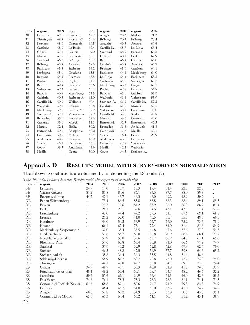
rank region 2009 region 2010 region 2011 region 2012 30 La Rioja 69.1 Saarland 69.7 Aragón 70.2 Molise 71.3 31 Thüringen 68.8 Nordr.-W. 69.6 Br'burg 70.2 Br'burg 70.4 32 Sachsen 68.0 Cantabria 69.5 Asturias 69.3 Aragón 69.6 33 Cataluña 68.0 La Rioja 69.4 Castilla L. 68.7 La Rioja 68.4 34 Galicia 67.9 Galicia 69.0 Saarland 68.6 Bremen 68.2 35 Molise 67.5 Basilicata 68.7 Galicia 68.0 Berlin 67.9 36 Saarland 66.8 Br'burg 68.7 Berlin 66.9 Galicia 66.0 37 Br'burg 66.8 Asturias 68.5 Cataluña 65.8 Asturias 64.7 38 Basilicata 65.5 Sachsen 66.2 Bremen 65.0 Cataluña 64.1 39 Sardegna 65.1 Cataluña 65.8 Basilicata 64.6 Meck'burg 64.0 40 Bremen 64.3 Bremen 65.5 La Rioja 64.2 Basilicata 63.5 41 Puglia 63.0 Puglia 64.7 Sardegna 64.1 Sardegna 62.2 42 Berlin 62.9 Calabria 63.6 Meck'burg 63.8 Puglia 62.1 43 Valenciana 62.3 Berlin 63.4 Puglia 62.6 Balears 56.8 44 Balears 60.6 Meck'burg 61.5 Balears 62.1 Calabria 55.9 45 Calabria 60.3 Sachsen-A. 61.0 Wallonia 61.6 Valenciana 53.9 46 Castilla M. 60.0 Wallonia 60.4 Sachsen-A. 61.6 Castilla M. 52.2 47 Wallonia 59.9 Balears 58.8 Calabria 61.1 Murcia 50.5 48 Meck'burg 59.5 Castilla M. 57.9 Valenciana 58.0 Campania 45.0 49 Sachsen-A. 57.7 Valenciana 57.2 Castilla M. 54.1 Sicilia 43.8 50 Bruxelles 55.1 Bruxelles 52.6 Murcia 53.0 Canarias 43.0 51 Canarias 53.1 Murcia 51.1 Extremad. 52.3 Extremad. 42.3 52 Murcia 52.4 Sicilia 50.2 Bruxelles 51.3 Andalucía 41.8 53 Extremad. 50.9 Campania 50.2 Campania 47.7 Melilla 30.1 54 Campania 50.5 Melilla 48.4 Sicilia 46.4 Ceuta 26.9 55 Andalucía 48.5 Canarias 46.9 Andalucía 43.1 Bruxelles 56 Sicilia 46.9 Extremad. 46.4 Canarias 42.6 Vlaams G. 57 Ceuta 33.3 Andalucía 45.9 Melilla 42.2 Wallonia 58 Melilla Ceuta 30.0 Ceuta 34.5 Sachsen-A.
RESULTS: MODEL WITH SURVEY-DRIVEN NORMALISATION The following coefficients are obtained by implementing the LS model (9) Table 19, Social Inclusion Measure, Baseline model with expert-based normalisation
nation region 2004 2005 2006 2007 2008 2009 2010 2011 2012 BE Bruxelles 24.9 17.0 17.7 18.3 17.4 31.4 22.5 22.8 . BE Vlaams Gewest 81.2 81.8 84.6 86.1 87.3 87.7 88.0 89.8 . BE Région wallonne 44.7 42.1 43.7 46.3 46.0 49.2 48.9 50.2 . DE Baden-Württemberg . 79.4 84.5 85.8 88.8 88.3 88.4 89.1 89.5 DE Bayern . 79.7 77.6 84.2 85.9 86.0 86.9 86.7 87.4 DE Berlin . 28.1 29.1 37.6 34.5 43.1 43.5 51.4 53.6 DE Brandenburg . 43.0 44.4 49.2 59.3 61.7 67.6 69.1 68.8 DE Bremen . 21.2 32.0 41.0 45.5 55.4 55.5 49.0 60.5 DE Hamburg . 44.0 54.3 53.9 67.7 76.0 75.2 73.5 75.9 DE Hessen . 66.1 67.4 73.1 77.4 81.0 81.4 83.6 84.9 DE Mecklenburg-Vorpommern . 32.0 35.4 38.5 44.8 47.6 52.6 57.2 54.5 DE Niedersachsen . 53.8 56.7 63.0 66.8 70.9 68.8 68.1 73.7 DE Nordrhein-Westfalen . 52.9 53.8 59.6 63.7 66.9 64.5 67.1 69.6 DE Rheinland-Pfalz . 57.6 62.8 67.4 73.8 71.0 66.6 71.2 74.7 DE Saarland . 37.9 40.2 62.9 62.8 62.8 69.3 62.4 70.0 DE Sachsen . 46.5 48.8 47.5 54.9 57.7 59.8 64.6 69.2 DE Sachsen-Anhalt . 35.8 36.4 36.3 35.5 44.8 51.4 48.6 DE Schleswig-Holstein . 58.9 61.7 69.7 70.8 75.0 73.2 74.0 75.0 DE Thüringen . 44.1 45.8 47.7 59.8 64.7 69.3 71.9 74.4 ES Galicia 34.9 48.7 47.1 50.3 48.8 51.8 45.5 36.8 32.9 ES Principado de Asturias 48.1 48.2 57.4 60.1 58.7 54.7 48.2 46.6 32.2 ES Cantabria 50.5 57.6 61.1 60.9 63.4 61.5 46.0 42.3 55.3 ES País Vasco 74.6 76.1 78.3 75.3 78.3 78.3 81.1 74.1 71.5 ES Comunidad Foral de Navarra 61.6 68.8 82.1 80.6 74.7 71.9 79.3 82.8 74.9 ES La Rioja . 46.4 48.7 51.0 50.0 53.5 45.0 34.7 34.8 ES Aragón 60.5 52.8 60.2 54.9 58.3 63.8 50.5 43.0 35.1 ES Comunidad de Madrid 65.3 61.3 64.4 63.2 61.1 60.4 51.2 45.1 38.9
29
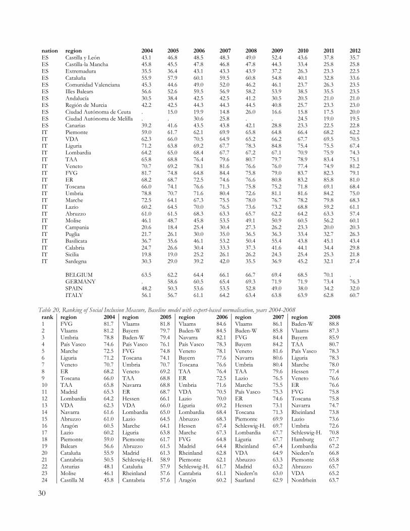
nation region 2004 2005 2006 2007 2008 2009 2010 2011 2012 ES Castilla y León 43.1 46.8 48.5 48.3 49.0 52.4 43.6 37.8 35.7 ES Castilla-la Mancha 45.8 45.5 47.8 46.8 47.8 44.3 33.4 25.8 25.8 ES Extremadura 35.5 36.4 43.1 43.3 43.9 37.2 26.3 23.3 22.5 ES Cataluña 55.9 57.9 60.1 59.5 60.8 54.8 40.1 32.8 33.6 ES Comunidad Valenciana 45.3 44.6 49.0 52.0 46.2 46.1 23.7 26.3 23.5 ES Illes Balears 56.6 52.6 59.5 56.9 58.2 53.9 38.5 35.5 23.5 ES Andalucía 30.5 38.4 42.5 42.5 41.2 30.5 20.5 21.0 21.0 ES Región de Murcia 42.2 42.5 44.3 44.3 44.5 40.8 25.7 23.3 23.0 ES Ciudad Autónoma de Ceuta . 15.0 19.9 14.8 26.0 16.6 15.8 17.5 20.0 ES Ciudad Autónoma de Melilla . . 30.6 25.8 . . 24.5 19.0 19.5 ES Canarias 39.2 41.6 43.5 43.8 42.1 28.8 23.3 22.5 22.8 IT Piemonte 59.0 61.7 62.1 69.9 65.8 64.8 66.4 68.2 62.2 IT VDA 62.3 66.0 70.5 64.9 65.2 66.2 67.7 69.5 70.5 IT Liguria 71.2 63.8 69.2 67.7 78.3 84.8 75.4 75.5 67.4 IT Lombardia 64.2 65.0 68.4 67.7 67.2 67.1 70.9 75.9 74.3 IT TAA 65.8 68.8 76.4 79.6 80.7 79.7 78.9 83.4 75.1 IT Veneto 70.7 69.2 78.1 81.6 76.6 76.0 77.4 74.9 81.2 IT FVG 81.7 74.8 64.8 84.4 75.8 79.0 83.7 82.3 79.1 IT ER 68.2 68.7 72.5 74.6 76.6 80.8 83.2 85.8 81.0 IT Toscana 66.0 74.1 76.6 71.3 75.8 75.2 71.8 69.1 68.4 IT Umbria 78.8 70.7 71.6 80.4 72.6 81.1 81.6 84.2 75.0 IT Marche 72.5 64.1 67.3 75.5 78.0 76.7 78.2 79.8 68.3 IT Lazio 60.2 64.5 70.0 76.5 73.6 73.2 68.8 59.2 61.1 IT Abruzzo 61.0 61.5 68.3 63.3 65.7 62.2 64.2 63.3 57.4 IT Molise 46.1 48.7 45.8 53.5 49.1 50.9 60.5 56.2 60.1 IT Campania 20.6 18.4 25.4 30.4 27.3 26.2 23.3 20.0 20.3 IT Puglia 21.7 26.1 30.0 35.0 36.5 36.3 33.4 32.7 26.3 IT Basilicata 36.7 35.6 46.1 53.2 50.4 55.4 43.8 45.1 43.4 IT Calabria 24.7 26.6 30.4 33.3 37.3 41.6 44.1 34.4 29.8 IT Sicilia 19.8 19.0 25.2 26.1 26.2 24.3 25.4 25.3 21.8 IT Sardegna 30.3 29.0 39.2 42.0 35.5 36.9 45.2 32.1 27.4 BELGIUM 63.5 62.2 64.4 66.1 66.7 69.4 68.5 70.1 . GERMANY . 58.6 60.5 65.4 69.3 71.9 71.9 73.4 76.3 SPAIN 48.2 50.3 53.6 53.5 52.8 49.0 38.0 34.2 32.0 ITALY 56.1 56.7 61.1 64.2 63.4 63.8 63.9 62.8 60.7
Table 20, Ranking of Social Inclusion Measure, Baseline model with expert-based normalisation, years 2004-2008
rank region 2004 region 2005 region 2006 region 2007 region 2008 1 FVG 81.7 Vlaams 81.8 Vlaams 84.6 Vlaams 86.1 Baden-W 88.8 2 Vlaams 81.2 Bayern 79.7 Baden-W 84.5 Baden-W 85.8 Vlaams 87.3 3 Umbria 78.8 Baden-W 79.4 Navarra 82.1 FVG 84.4 Bayern 85.9 4 País Vasco 74.6 País Vasco 76.1 País Vasco 78.3 Bayern 84.2 TAA 80.7 5 Marche 72.5 FVG 74.8 Veneto 78.1 Veneto 81.6 País Vasco 78.3 6 Liguria 71.2 Toscana 74.1 Bayern 77.6 Navarra 80.6 Liguria 78.3 7 Veneto 70.7 Umbria 70.7 Toscana 76.6 Umbria 80.4 Marche 78.0 8 ER 68.2 Veneto 69.2 TAA 76.4 TAA 79.6 Hessen 77.4 9 Toscana 66.0 TAA 68.8 ER 72.5 Lazio 76.5 Veneto 76.6 10 TAA 65.8 Navarra 68.8 Umbria 71.6 Marche 75.5 ER 76.6 11 Madrid 65.3 ER 68.7 VDA 70.5 País Vasco 75.3 FVG 75.8 12 Lombardia 64.2 Hessen 66.1 Lazio 70.0 ER 74.6 Toscana 75.8 13 VDA 62.3 VDA 66.0 Liguria 69.2 Hessen 73.1 Navarra 74.7 14 Navarra 61.6 Lombardia 65.0 Lombardia 68.4 Toscana 71.3 Rheinland 73.8 15 Abruzzo 61.0 Lazio 64.5 Abruzzo 68.3 Piemonte 69.9 Lazio 73.6 16 Aragón 60.5 Marche 64.1 Hessen 67.4 Schleswig-H. 69.7 Umbria 72.6 17 Lazio 60.2 Liguria 63.8 Marche 67.3 Lombardia 67.7 Schleswig-H. 70.8 18 Piemonte 59.0 Piemonte 61.7 FVG 64.8 Liguria 67.7 Hamburg 67.7 19 Balears 56.6 Abruzzo 61.5 Madrid 64.4 Rheinland 67.4 Lombardia 67.2 20 Cataluña 55.9 Madrid 61.3 Rheinland 62.8 VDA 64.9 Nieders'n 66.8 21 Cantabria 50.5 Schleswig-H. 58.9 Piemonte 62.1 Abruzzo 63.3 Piemonte 65.8 22 Asturias 48.1 Cataluña 57.9 Schleswig-H. 61.7 Madrid 63.2 Abruzzo 65.7 23 Molise 46.1 Rheinland 57.6 Cantabria 61.1 Nieders'n 63.0 VDA 65.2 24 Castilla M 45.8 Cantabria 57.6 Aragón 60.2 Saarland 62.9 Nordrhein 63.7
30
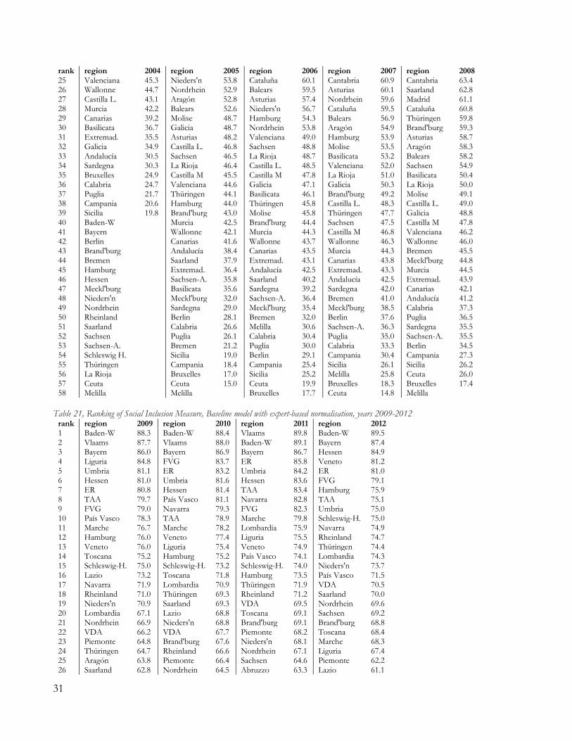
rank region 2004 region 2005 region 2006 region 2007 region 2008 25 Valenciana 45.3 Nieders'n 53.8 Cataluña 60.1 Cantabria 60.9 Cantabria 63.4 26 Wallonne 44.7 Nordrhein 52.9 Balears 59.5 Asturias 60.1 Saarland 62.8 27 Castilla L. 43.1 Aragón 52.8 Asturias 57.4 Nordrhein 59.6 Madrid 61.1 28 Murcia 42.2 Balears 52.6 Nieders'n 56.7 Cataluña 59.5 Cataluña 60.8 29 Canarias 39.2 Molise 48.7 Hamburg 54.3 Balears 56.9 Thüringen 59.8 30 Basilicata 36.7 Galicia 48.7 Nordrhein 53.8 Aragón 54.9 Brand'burg 59.3 31 Extremad. 35.5 Asturias 48.2 Valenciana 49.0 Hamburg 53.9 Asturias 58.7 32 Galicia 34.9 Castilla L. 46.8 Sachsen 48.8 Molise 53.5 Aragón 58.3 33 Andalucía 30.5 Sachsen 46.5 La Rioja 48.7 Basilicata 53.2 Balears 58.2 34 Sardegna 30.3 La Rioja 46.4 Castilla L. 48.5 Valenciana 52.0 Sachsen 54.9 35 Bruxelles 24.9 Castilla M 45.5 Castilla M 47.8 La Rioja 51.0 Basilicata 50.4 36 Calabria 24.7 Valenciana 44.6 Galicia 47.1 Galicia 50.3 La Rioja 50.0 37 Puglia 21.7 Thüringen 44.1 Basilicata 46.1 Brand'burg 49.2 Molise 49.1 38 Campania 20.6 Hamburg 44.0 Thüringen 45.8 Castilla L. 48.3 Castilla L. 49.0 39 Sicilia 19.8 Brand'burg 43.0 Molise 45.8 Thüringen 47.7 Galicia 48.8 40 Baden-W Murcia 42.5 Brand'burg 44.4 Sachsen 47.5 Castilla M 47.8 41 Bayern Wallonne 42.1 Murcia 44.3 Castilla M 46.8 Valenciana 46.2 42 Berlin Canarias 41.6 Wallonne 43.7 Wallonne 46.3 Wallonne 46.0 43 Brand'burg Andalucía 38.4 Canarias 43.5 Murcia 44.3 Bremen 45.5 44 Bremen Saarland 37.9 Extremad. 43.1 Canarias 43.8 Meckl'burg 44.8 45 Hamburg Extremad. 36.4 Andalucía 42.5 Extremad. 43.3 Murcia 44.5 46 Hessen Sachsen-A. 35.8 Saarland 40.2 Andalucía 42.5 Extremad. 43.9 47 Meckl'burg Basilicata 35.6 Sardegna 39.2 Sardegna 42.0 Canarias 42.1 48 Nieders'n Meckl'burg 32.0 Sachsen-A. 36.4 Bremen 41.0 Andalucía 41.2 49 Nordrhein Sardegna 29.0 Meckl'burg 35.4 Meckl'burg 38.5 Calabria 37.3 50 Rheinland Berlin 28.1 Bremen 32.0 Berlin 37.6 Puglia 36.5 51 Saarland Calabria 26.6 Melilla 30.6 Sachsen-A. 36.3 Sardegna 35.5 52 Sachsen Puglia 26.1 Calabria 30.4 Puglia 35.0 Sachsen-A. 35.5 53 Sachsen-A. Bremen 21.2 Puglia 30.0 Calabria 33.3 Berlin 34.5 54 Schleswig H. Sicilia 19.0 Berlin 29.1 Campania 30.4 Campania 27.3 55 Thüringen Campania 18.4 Campania 25.4 Sicilia 26.1 Sicilia 26.2 56 La Rioja Bruxelles 17.0 Sicilia 25.2 Melilla 25.8 Ceuta 26.0 57 Ceuta Ceuta 15.0 Ceuta 19.9 Bruxelles 18.3 Bruxelles 17.4 58 Melilla Melilla Bruxelles 17.7 Ceuta 14.8 Melilla
Table 21, Ranking of Social Inclusion Measure, Baseline model with expert-based normalisation, years 2009-2012
rank region 2009 region 2010 region 2011 region 2012 1 Baden-W 88.3 Baden-W 88.4 Vlaams 89.8 Baden-W 89.5 2 Vlaams 87.7 Vlaams 88.0 Baden-W 89.1 Bayern 87.4 3 Bayern 86.0 Bayern 86.9 Bayern 86.7 Hessen 84.9 4 Liguria 84.8 FVG 83.7 ER 85.8 Veneto 81.2 5 Umbria 81.1 ER 83.2 Umbria 84.2 ER 81.0 6 Hessen 81.0 Umbria 81.6 Hessen 83.6 FVG 79.1 7 ER 80.8 Hessen 81.4 TAA 83.4 Hamburg 75.9 8 TAA 79.7 País Vasco 81.1 Navarra 82.8 TAA 75.1 9 FVG 79.0 Navarra 79.3 FVG 82.3 Umbria 75.0 10 País Vasco 78.3 TAA 78.9 Marche 79.8 Schleswig-H. 75.0 11 Marche 76.7 Marche 78.2 Lombardia 75.9 Navarra 74.9 12 Hamburg 76.0 Veneto 77.4 Liguria 75.5 Rheinland 74.7 13 Veneto 76.0 Liguria 75.4 Veneto 74.9 Thüringen 74.4 14 Toscana 75.2 Hamburg 75.2 País Vasco 74.1 Lombardia 74.3 15 Schleswig-H. 75.0 Schleswig-H. 73.2 Schleswig-H. 74.0 Nieders'n 73.7 16 Lazio 73.2 Toscana 71.8 Hamburg 73.5 País Vasco 71.5 17 Navarra 71.9 Lombardia 70.9 Thüringen 71.9 VDA 70.5 18 Rheinland 71.0 Thüringen 69.3 Rheinland 71.2 Saarland 70.0 19 Nieders'n 70.9 Saarland 69.3 VDA 69.5 Nordrhein 69.6 20 Lombardia 67.1 Lazio 68.8 Toscana 69.1 Sachsen 69.2 21 Nordrhein 66.9 Nieders'n 68.8 Brand'burg 69.1 Brand'burg 68.8 22 VDA 66.2 VDA 67.7 Piemonte 68.2 Toscana 68.4 23 Piemonte 64.8 Brand'burg 67.6 Nieders'n 68.1 Marche 68.3 24 Thüringen 64.7 Rheinland 66.6 Nordrhein 67.1 Liguria 67.4 25 Aragón 63.8 Piemonte 66.4 Sachsen 64.6 Piemonte 62.2 26 Saarland 62.8 Nordrhein 64.5 Abruzzo 63.3 Lazio 61.1
31
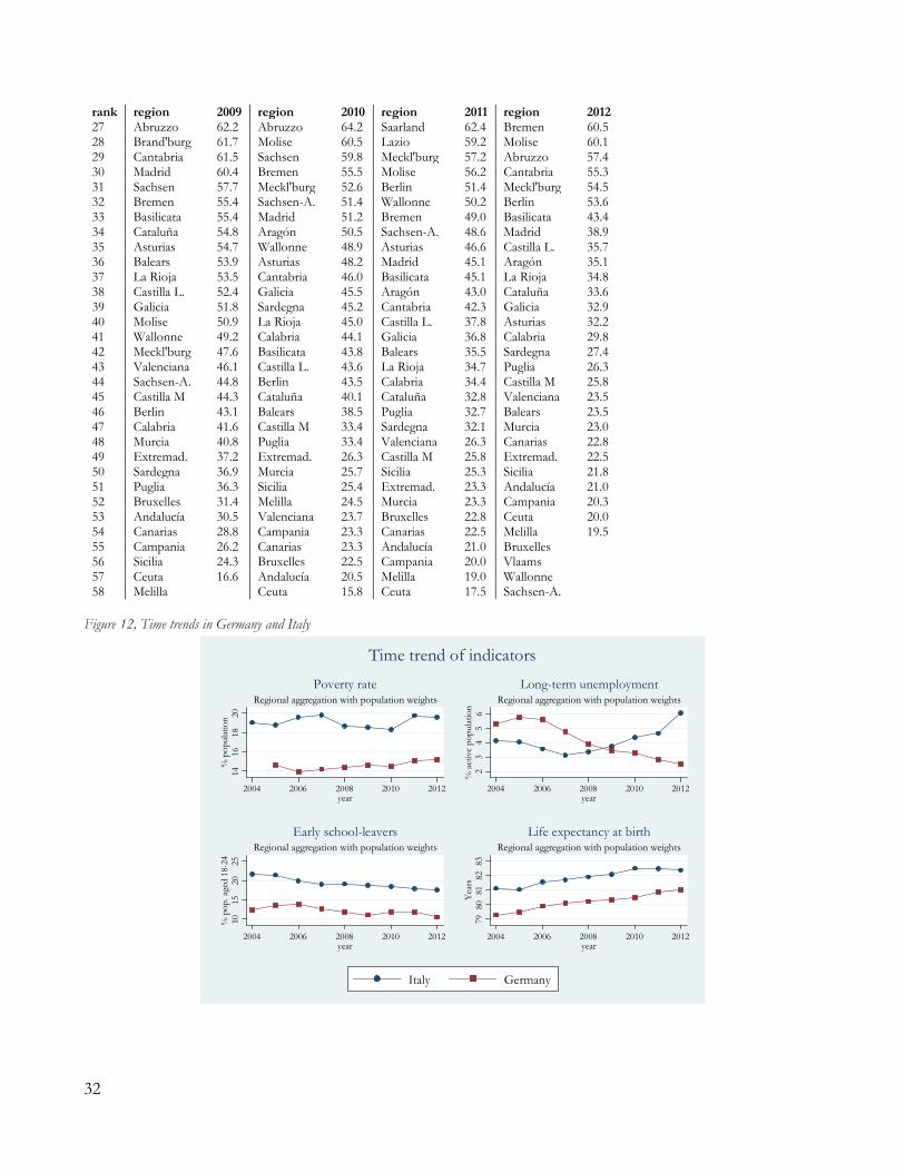
rank region 2009 region 2010 region 2011 region 2012 27 Abruzzo 62.2 Abruzzo 64.2 Saarland 62.4 Bremen 60.5 28 Brand'burg 61.7 Molise 60.5 Lazio 59.2 Molise 60.1 29 Cantabria 61.5 Sachsen 59.8 Meckl'burg 57.2 Abruzzo 57.4 30 Madrid 60.4 Bremen 55.5 Molise 56.2 Cantabria 55.3 31 Sachsen 57.7 Meckl'burg 52.6 Berlin 51.4 Meckl'burg 54.5 32 Bremen 55.4 Sachsen-A. 51.4 Wallonne 50.2 Berlin 53.6 33 Basilicata 55.4 Madrid 51.2 Bremen 49.0 Basilicata 43.4 34 Cataluña 54.8 Aragón 50.5 Sachsen-A. 48.6 Madrid 38.9 35 Asturias 54.7 Wallonne 48.9 Asturias 46.6 Castilla L. 35.7 36 Balears 53.9 Asturias 48.2 Madrid 45.1 Aragón 35.1 37 La Rioja 53.5 Cantabria 46.0 Basilicata 45.1 La Rioja 34.8 38 Castilla L. 52.4 Galicia 45.5 Aragón 43.0 Cataluña 33.6 39 Galicia 51.8 Sardegna 45.2 Cantabria 42.3 Galicia 32.9 40 Molise 50.9 La Rioja 45.0 Castilla L. 37.8 Asturias 32.2 41 Wallonne 49.2 Calabria 44.1 Galicia 36.8 Calabria 29.8 42 Meckl'burg 47.6 Basilicata 43.8 Balears 35.5 Sardegna 27.4 43 Valenciana 46.1 Castilla L. 43.6 La Rioja 34.7 Puglia 26.3 44 Sachsen-A. 44.8 Berlin 43.5 Calabria 34.4 Castilla M 25.8 45 Castilla M 44.3 Cataluña 40.1 Cataluña 32.8 Valenciana 23.5 46 Berlin 43.1 Balears 38.5 Puglia 32.7 Balears 23.5 47 Calabria 41.6 Castilla M 33.4 Sardegna 32.1 Murcia 23.0 48 Murcia 40.8 Puglia 33.4 Valenciana 26.3 Canarias 22.8 49 Extremad. 37.2 Extremad. 26.3 Castilla M 25.8 Extremad. 22.5 50 Sardegna 36.9 Murcia 25.7 Sicilia 25.3 Sicilia 21.8 51 Puglia 36.3 Sicilia 25.4 Extremad. 23.3 Andalucía 21.0 52 Bruxelles 31.4 Melilla 24.5 Murcia 23.3 Campania 20.3 53 Andalucía 30.5 Valenciana 23.7 Bruxelles 22.8 Ceuta 20.0 54 Canarias 28.8 Campania 23.3 Canarias 22.5 Melilla 19.5 55 Campania 26.2 Canarias 23.3 Andalucía 21.0 Bruxelles 56 Sicilia 24.3 Bruxelles 22.5 Campania 20.0 Vlaams 57 Ceuta 16.6 Andalucía 20.5 Melilla 19.0 Wallonne 58 Melilla Ceuta 15.8 Ceuta 17.5 Sachsen-A.
Figure 12, Time trends in Germany and Italy
1416
1820
% p
opul
atio
n
2004 2006 2008 2010 2012year
Regional aggregation with population weightsPoverty rate
23
45
6%
act
ive
popu
latio
n
2004 2006 2008 2010 2012year
Regional aggregation with population weightsLong-term unemployment
1015
2025
% p
op. a
ged
18-2
4
2004 2006 2008 2010 2012year
Regional aggregation with population weightsEarly school-leavers
7980
8182
83Y
ears
2004 2006 2008 2010 2012year
Regional aggregation with population weightsLife expectancy at birth
Time trend of indicators
Italy Germany
32
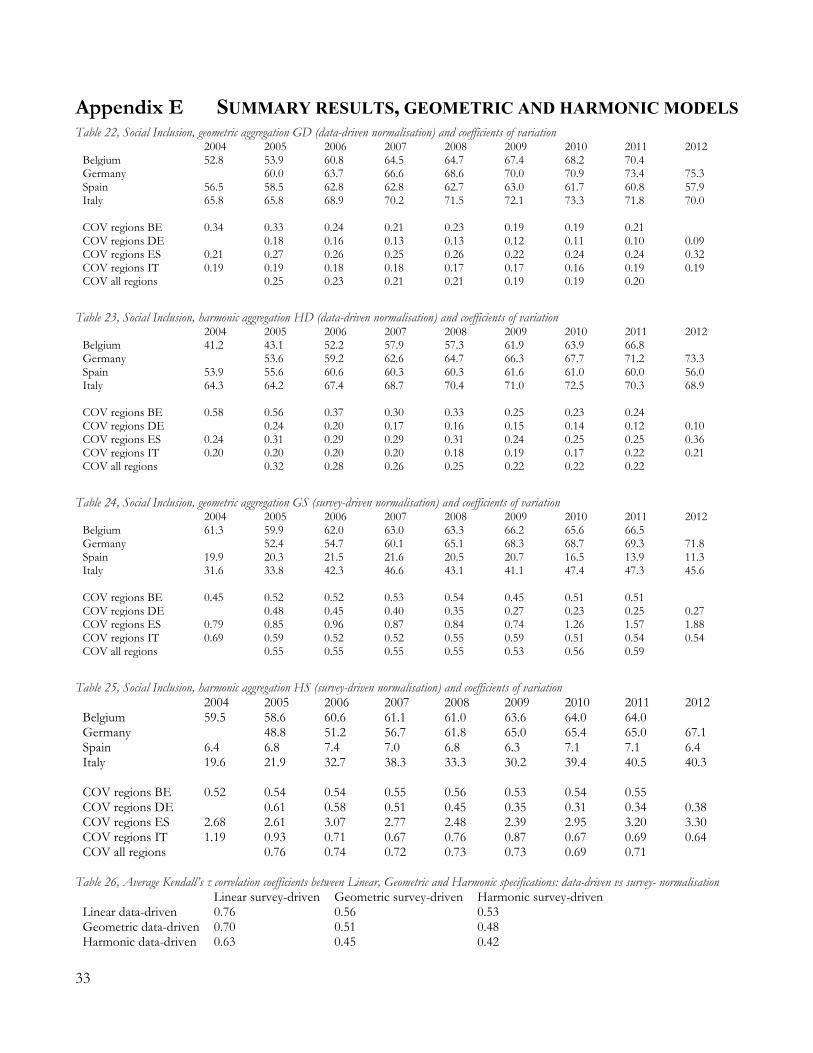
SUMMARY RESULTS, GEOMETRIC AND HARMONIC MODELS Table 22, Social Inclusion, geometric aggregation GD (data-driven normalisation) and coefficients of variation
2004 2005 2006 2007 2008 2009 2010 2011 2012 Belgium 52.8 53.9 60.8 64.5 64.7 67.4 68.2 70.4 Germany 60.0 63.7 66.6 68.6 70.0 70.9 73.4 75.3 Spain 56.5 58.5 62.8 62.8 62.7 63.0 61.7 60.8 57.9 Italy 65.8 65.8 68.9 70.2 71.5 72.1 73.3 71.8 70.0 COV regions BE 0.34 0.33 0.24 0.21 0.23 0.19 0.19 0.21 COV regions DE 0.18 0.16 0.13 0.13 0.12 0.11 0.10 0.09 COV regions ES 0.21 0.27 0.26 0.25 0.26 0.22 0.24 0.24 0.32 COV regions IT 0.19 0.19 0.18 0.18 0.17 0.17 0.16 0.19 0.19 COV all regions 0.25 0.23 0.21 0.21 0.19 0.19 0.20
Table 23, Social Inclusion, harmonic aggregation HD (data-driven normalisation) and coefficients of variation
2004 2005 2006 2007 2008 2009 2010 2011 2012 Belgium 41.2 43.1 52.2 57.9 57.3 61.9 63.9 66.8 Germany 53.6 59.2 62.6 64.7 66.3 67.7 71.2 73.3 Spain 53.9 55.6 60.6 60.3 60.3 61.6 61.0 60.0 56.0 Italy 64.3 64.2 67.4 68.7 70.4 71.0 72.5 70.3 68.9 COV regions BE 0.58 0.56 0.37 0.30 0.33 0.25 0.23 0.24 COV regions DE 0.24 0.20 0.17 0.16 0.15 0.14 0.12 0.10 COV regions ES 0.24 0.31 0.29 0.29 0.31 0.24 0.25 0.25 0.36 COV regions IT 0.20 0.20 0.20 0.20 0.18 0.19 0.17 0.22 0.21 COV all regions 0.32 0.28 0.26 0.25 0.22 0.22 0.22
Table 24, Social Inclusion, geometric aggregation GS (survey-driven normalisation) and coefficients of variation
2004 2005 2006 2007 2008 2009 2010 2011 2012 Belgium 61.3 59.9 62.0 63.0 63.3 66.2 65.6 66.5 Germany 52.4 54.7 60.1 65.1 68.3 68.7 69.3 71.8 Spain 19.9 20.3 21.5 21.6 20.5 20.7 16.5 13.9 11.3 Italy 31.6 33.8 42.3 46.6 43.1 41.1 47.4 47.3 45.6 COV regions BE 0.45 0.52 0.52 0.53 0.54 0.45 0.51 0.51 COV regions DE 0.48 0.45 0.40 0.35 0.27 0.23 0.25 0.27 COV regions ES 0.79 0.85 0.96 0.87 0.84 0.74 1.26 1.57 1.88 COV regions IT 0.69 0.59 0.52 0.52 0.55 0.59 0.51 0.54 0.54 COV all regions 0.55 0.55 0.55 0.55 0.53 0.56 0.59
Table 25, Social Inclusion, harmonic aggregation HS (survey-driven normalisation) and coefficients of variation
2004 2005 2006 2007 2008 2009 2010 2011 2012 Belgium 59.5 58.6 60.6 61.1 61.0 63.6 64.0 64.0 Germany 48.8 51.2 56.7 61.8 65.0 65.4 65.0 67.1 Spain 6.4 6.8 7.4 7.0 6.8 6.3 7.1 7.1 6.4 Italy 19.6 21.9 32.7 38.3 33.3 30.2 39.4 40.5 40.3 COV regions BE 0.52 0.54 0.54 0.55 0.56 0.53 0.54 0.55 COV regions DE 0.61 0.58 0.51 0.45 0.35 0.31 0.34 0.38 COV regions ES 2.68 2.61 3.07 2.77 2.48 2.39 2.95 3.20 3.30 COV regions IT 1.19 0.93 0.71 0.67 0.76 0.87 0.67 0.69 0.64 COV all regions 0.76 0.74 0.72 0.73 0.73 0.69 0.71
Table 26, Average Kendall’s τ correlation coefficients between Linear, Geometric and Harmonic specifications: data-driven vs survey- normalisation
Linear survey-driven Geometric survey-driven Harmonic survey-driven Linear data-driven 0.76 0.56 0.53 Geometric data-driven 0.70 0.51 0.48 Harmonic data-driven 0.63 0.45 0.42
33