Luxembourg Income Study

Working Paper Series

Luxembourg Income Study (LIS), asbl

Working Paper No. 551

Tax Progression: International and Intertemporal Comparisons

Using LIS Data

Kirill Pogorelskiy, Christian Seidl and Stefan Traub

September 2010

TAX PROGRESSION: INTERNATIONAL AND

INTERTEMPORAL COMPARISONS USING LIS DATA

by Kirill Pogorelskiy∗, Christian Seidl∗∗, and Stefan Traub‡

Revised Version: September 2010

Abstract

The conventional approach to comparing tax progression (using local measures, global measures ordominance relations for �rst moment distribution functions) often lacks applicability to the real world:local measures of tax progression have the disadvantage of ignoring the income distribution entirely.Global measures are a�ected by the drawback of all aggregation, viz. ignoring structural di�erencesbetween the objects to be compared. Dominance relations of comparing tax progression depend heavilyon the assumption that the same income distribution holds for both situations to be compared, whichrenders this approach impossible for international and intertemporal comparisons.

Based on the earlier work of one of the authors, this paper develops a uni�ed methodology to comparetax progression for dominance relations under di�erent income distributions. We address it as uniformtax progression for di�erent income distributions and present the respective approach for both continuousand discrete cases, the latter also being employed for empirical investigations.

Using dominance relations, we de�ne tax progression under di�erent income distributions as a classof natural extensions of uniform tax progression in terms of taxes, net incomes, and di�erences of �rstmoment distribution functions. To cope with di�erent monetary units and di�erent supports of theincome distributions involved, we utilized their transformations to population and income quantiles.Altogether, we applied six methods of comparing tax progression, three in terms of taxes and threein terms of net incomes, which we utilized for empirical analyses of comparisons of tax progressionusing data from the Luxembourg Income Study. This is the �rst paper that performs international andintertemporal comparisons of uniform tax progression with actual data.

For our analysis we chose those countries for which LIS disposes of data on gross incomes, taxes,payroll taxes and net incomes. This pertains to 15 countries, out of which we selected 13. This gaverise to 78 international comparisons, which we carried out for household data, equivalized data, directtaxes and direct taxes inclusive of payroll taxes. In total we investigated 312 international comparisonsfor each of the six methods of comparing tax progression.

In two thirds of all cases we observed uniformly greater tax progression for international comparisons.In a bit more than one �fth of all cases we observed bifurcate tax progression, that is, progression ishigher for one country up to some population or income quantile threshold, beyond which the situationis the opposite, i.e., progression is higher for the second country. No clear-cut �ndings can be reportedfor just one tenth of all cases. But even in these cases some curve di�erences are so small that they maywell be ignored.

We also test consistency of our results with regard to the six methods of comparing tax progressionand present here twelve (Germany, the UK and the US) plus four comparing Germany and Sweden outof the total of 312 graphs, each containing six di�erences of �rst moment distribution functions. Thesedi�erences can be interpreted as intensity of greater tax progression. We demonstrate the overall pictureof uniform tax progression for international comparisons using Hasse diagrams.

Concerning intertemporal comparisons of tax progression, we present the results for the US, the UK,and Germany for several time periods. We align our �ndings with respect to major political eras in thesecountries, e.g., G. Bush senior, W. Clinton, and G. Bush junior for the United States; M. Thatcher, J.Major, and A. Blair for the United Kingdom, and for Germany, the last year before German re-uni�cation(1989), the beginning of H. Kohl's last term as chancellor (1994), and G. Schröder (2000). In addition,we study sensitivity of our results to the equivalence scale parameter.

JEL Classi�cation: H23, H24.Keywords: income tax progression, measurement of uniform tax progression, comparisons of tax pro-gression, tax progression with di�erent income distributions.

∗State University � Higher School of Economics, Moscow, Russia; kirill.pogorelskiy@gmail.com∗∗University of Kiel, Germany; seidl@economics.uni-kiel.de‡University of Bremen, Germany; traub@uni-bremen.de

1 Introduction

Tax progression has ever been of concern, not only to the profession, but also to politi-

cians, let alone to the man on the street. Hence, measurement of tax progression and

international as well as intertemporal comparisons of tax progression are of utmost im-

portance. Intuitively, by tax progression we mean a situation when, as income increases,

so does the average tax rate, i.e., the higher income strata pay a relatively larger share of

their gross income than the lower income strata do. If we take the tax system as a whole,

then in addition to the tax schedule we should also take into account the in�uence of

the existing income distribution in order to be able to draw sound conclusions about its

real progression. Thus, we agree with Suits (1977, p. 725): �There is nothing inherently

regressive about a sales tax or even a poll tax. They are regressive because income is

unequally distributed, and the more unequally income is distributed, the more regressive

they become.�

In contrast to that, the existing methodology of measuring and comparing tax pro-

gression allows only answers to problems which are outside central interest. There are

three main routes of research, viz. local, global, and uniform measures of tax progression.

Local measures of tax progression, in particular its main representatives, tax revenue elas-

ticity and residual income elasticity, concentrate on the tax schedule only and neglect the

important role of the income distribution for tax progression. If a certain tax schedule

happens to be rather progressive but hits very few people only, then the respective tax

system should not be viewed as highly progressive. Global measures of tax progression

weigh taxation or the net incomes by the income distribution in addition to some other

weights, but this very aggregation procedure is its main drawback. A tax schedule which

is regressive over some income intervals may be categorized to be more progressive than

another tax schedule which is progressive throughout just because of compensation due

to the aggregation procedure. Uniform measures of tax progression which work by way

of single-crossing conditions or by relative concentration curves require the same income

distributions for all cases to be compared. This means that questions such as �Is the tax

schedule of the USA associated with the American income distribution more or less pro-

gressive than the German tax schedule associated with the German income distribution?�

cannot be answered by using this approach.

To handle these realistic problems, Seidl (1994) developed an approach in which com-

parisons are based on population quantiles or income quantiles with respect to taxes or

net incomes rather than on tax schedules directly in terms of income. This method allows

to substitute the income distributions with di�erent supports by quantiles with the unit

interval as the common support of di�erent distributions. The idea of this approach is

the following: if a tax schedule for one country collects relatively less tax revenue from

the lower income strata than does a tax schedule of another country, then the �rst one

is considered as more progressive. Alternatively, if the �rst tax schedule leaves the lower

income strata relatively more net income than does the tax schedule of another country,

1

then the �rst tax schedule is considered as more progressive. The comparison of these

relative positions is carried out in terms of the tax quantiles for the population quantiles

or for the income quantiles.1 In his theoretical work, Seidl (1994) made use of concavity

or convexity conditions of relative concentration curves, which, however, yielded only suf-

�cient conditions in terms of elasticities, but not necessary conditions of uniformly more

or less tax progression. It seems that no general analytic solution to this problem exists.2

The main purpose of this paper is an empirical investigation of international and

intertemporal comparisons of tax progression utilizing this approach. We used data from

the Luxembourg Income Study, LIS (2010), for 13 out of 15 countries for which data for

gross incomes, direct taxes, payroll taxes and net incomes are available (see Table 1 in

Section 4.1). We made separate comparisons for household incomes and for equivalized

incomes (using the Luxembourg equivalence scale) and for progression of direct taxes

and direct taxes plus payroll taxes (mainly comprising the employees' share of social

security contributions). This gave us four times 78 international comparisons. Moreover,

we applied six measurement devices for comparisons of tax progression, four in terms of

population quantiles and two in terms of income quantiles. In addition to that, we also

investigated intertemporal comparisons of tax progression for some selected countries and

studied the in�uence of the scale parameter of the Luxembourg equivalence scales on the

results of comparisons of tax progression.

Section 2 reviews local and global measures of tax progression, Section 3 deals with

uniform tax progression, �rst for identical income distributions (or, more generally, for

income distributions with the same support), which represents the customary theory,

second for di�erent income distributions in the continuous version, and third for di�erent

income distributions in the discrete version in preparation for empirical investigations.

Section 4 displays the results of our research. This section section starts with a descrip-

tion of LIS data and the procedures we applied to them; it continues by providing some

intuition about working with grouped data, and then proceeds with an elaborate discus-

sion of the results of our research. Except for one table and two �gures, all tables and

�gures are placed at the end of the paper.

1Dardanoni and Lambert (2002) took a di�erent route: rather than replacing incomes by quantiles,

they transplanted the income distributions by deformation functions (p. 102), thereby remaining in the

domain of incomes. For instance, when comparing the United States with Germany, they propose de-

forming the German income distribution to the American income distribution and look whether the

American tax system, when applied to the deformed compound distribution, is more or less progressive

than the American tax system as applied to the American income distribution. Alternatively, the Amer-

ican income distribution can be deformed to the German income distribution, or both distributions can

be deformed to a �ctive third income distribution.2Note that by a �general analytic solution� we mean the one that yields non-trivial necessary and

su�cient conditions. For instance, it is immediate that there is uniformly greater progression if and

only if the curve obtained by taking the di�erences of the transformed �rst moment curves of taxes

or net incomes does not change its sign within the unit interval. This condition, however, is a mere

reformulation of the de�nition of uniform tax progression (see Section 3.3).

2

2 Local and Global Measures of Tax Progression

This paper employs the following notation: Y denotes income, [Y∗, Y∗] denotes the sup-

port of the income distribution, f(Y ) ≥ 0 denotes the density function and F (Y ) the

distribution function of the income distribution, q denotes the population quantiles and

p the income quantiles of gross incomes, µ :=∫ Y ∗

Y∗Y f(Y )dY denotes mean gross income,

T (Y ) denotes the income tax schedule, T (Y )Y

denotes the average income tax schedule,dT (Y )dY

denotes the marginal income tax schedule,3 and τ :=∫ Y ∗

Y∗T (Y )f(Y )dY denotes

mean tax.

Local measures of income tax progression just focus on the tax schedule. The more

primitive ones are the �rst derivative of the average tax schedule and the di�erence of the

marginal and the average tax schedules. They are positive for progressive and negative

for regressive tax schedules. More re�ned measures are the tax elasticity

ε(Y ) :=dT (Y )/dY

T (Y )/Y

and the residual income elasticity

η(Y ) :=d[Y − T (Y )]/dY

[Y − T (Y )]/Y.

Verbally expressed, the tax elasticity is the ratio of marginal and average tax rates,

and the residual income elasticity is the ratio of the marginal and the average retention

rates. ε(y) measures liability progression, η(y) residual income progression. According to

liability progression, a tax schedule is progressive at Y if ε(Y ) > 1; according to residual

income progression a tax schedule is progressive at Y if 0 < η(Y ) < 1. The meaning of

these two local measures of tax progression is simple: ε(Y ) > 1 means that the tax on an

extra monetary unit for a taxpayer with income Y exceeds his or her average tax burden;

0 < η(Y ) < 1 means that an extra monetary unit leaves a taxpayer less net income than

under his or her average retention rate. Note that both measures are equivalent for the

general diagnosis of tax progression, that is, we have ε(Y ) > 1 ⇔ 0 < η(Y ) < 1, but

this equivalence does not apply to comparisons of tax progression. This means that for

two tax schedules T 1(Y ) and T 2(Y ) it does not follow that ε1(Y ) > ε2(Y ) holds if and

only if η1(Y ) < η2(Y ) holds. For a numerical illustration on a former German income

tax reform see Seidl and Kaletha (1987).

Local measures of tax progression have a crucial drawback: they are completely sep-

arated from income distributions. Hence, the fractions of people a�ected by the various

parts of a tax schedule are neglected by local measures of tax progression. Yet for com-

paring two situations with respect to tax progression on the whole, the fractions of the

population a�ected by the various parts of a tax schedule are important. Suppose that a

3For the sake of mathematical convenience we assume that all tax schedules are continuously di�er-

entiable.

3

tax schedule is very progressive, yet nobody in a society is a�ected by the very high rates

of this tax schedule. Then this tax schedule will be perceived as less progressive than a

tax schedule with more moderate rates which, however, cut in broad strata of taxpayers.

For an arbitrary income distribution (but which is assumed to be the same for both

schedules under comparison) we can employ local measures of tax progression for purposes

of progression comparison if we have dominance relationships throughout, e.g., ε1(Y ) >

ε2(Y ) or η1(Y ) < η2(Y ) for all Y ∈ [Y∗, Y∗]. If these relationships apply, then greater

tax progression of tax schedules holds trivially for any such income distribution on which

both tax schedules operate, and is therefore independent of the choice of the income

distribution. We will see below that similar relations represent su�cient conditions for

greater tax progression for uniform tax progression. Note that they may, although more

complicated, also be expressed in terms of q and p; we will come to these expressions

below.

The introduction of income distributions into comparisons of tax progression can be

done in two ways: the �rst one takes the route of aggregate measures which map taxes

and incomes into the real numbers�these are global measures of tax progression; the

second one uses dominance relations�these are measures of uniform tax progression.

Global measures of tax progression are based on income distribution measures of

gross incomes, net incomes, and taxes.4 In the simplest cases the Gini coe�cient is used.

Examples include, inter alia, the measure proposed by Dalton (1922/1954, pp. 107-8) as

the mean deviation of average tax rates (which is just the Gini coe�cient of the average

tax rates), or the measure proposed by Reynolds and Smolensky (1977), which is simply

the di�erence of the Gini coe�cients of net and gross incomes. Pechman and Okner

(1974) and Okner (1975) proposed to normalize the Reynolds-Smolensky measure by the

Gini coe�cient of gross incomes. The Musgrave and Thin (1948) measure of e�ective

progression is the ratio of the areas under the Lorenz curves for gross and net incomes.5

Many more global measures of tax progression were developed, e.g., by Hainsworth (1984),

Khetan and Poddar (1976), Suits (1977), Kakwani (1977b, 1984, 1987), Formby et al.

(1981, 1984), Pfähler (1982, 1983, 1987), Liu (1984), and Lambert (1988). Blackorby and

Donaldson (1984) and Kiefer (1984, pp. 500-1) chose another way: they proposed global

measures of tax progression based on the equally distributed equivalent income.

Pfähler (1987, p. 7), suggested a general framework for global measures of tax pro-

gression. He showed that most of the measures based on distributional measures can

4For short surveys see Kiefer (1984, pp. 498-9), Seidl (1994, pp. 343-6), and Peichl and Schäfer (2008,

pp. 3-5). Kiefer (1984, p. 497) distinguished two groups of global measures of tax progression, viz.

structural indices, which are functions of incomes and their respective taxes, and distributional indices,

which are functions of the tax structure and the distribution of post-tax incomes. If this classi�cation

is extended to measures of uniform tax progression, then our De�nitions 1, 2, and 5 in Section 3.3 are

structural measures of tax progression, and De�nitions 3, 4, and 6 are distributional measures of tax

progression.5The area under the Lorenz curve is one minus the Gini coe�cient divided by two.

4

be expressed as the weighted sum of local relative deviations [T (Y ) − τµY ]/τ of the

actual tax schedule from a revenue-neutral proportional tax schedule. For the expres-

sion of the global progression measures in terms of di�erences between the distribu-

tions of net incomes and gross incomes, Pfähler (1987, p. 12) showed that they can be

de�ned using the very same weights for the weighted sum of local relative deviations

[Y − T (Y )− (1− τµ)Y ]/(µ− τ) of actual net incomes from revenue-neutral net incomes

under a proportional tax.6

Global measures of tax progression not only serve to categorize tax schedules into

progressive, proportional and regressive, but also to derive an ordering of tax progression.

If progression is measured in terms of positive (negative) values, then tax schedule T 1(·)is more progressive than T 2(·) if the global measure applied shows a higher (lower) value

for T 1(·) than for T 2(·).Global measures of tax progression have several advantages. First, they work for

di�erent tax schedules and di�erent income distributions. This means that international

and intertemporal comparisons of tax progression can be e�ectuated. Second, they feature

a double weighting, both by some weights particular to the speci�c global measure, and

by the income distribution. That is, particular characteristics of a tax schedule gain

more (less) weight if more (less) taxpayers are a�ected. Third, global measures of tax

progression are able to compensate income subintervals with opposite properties of tax

schedules by appropriate weighting and subsequent aggregation.

However, at the same time this last advantage turns out as a major handicap of

global measures of tax progression. Aggregating the e�ects of tax schedules over the

whole support of the income distribution may lead to the result that T 1(·) is categorizedas being more progressive than T 2(·), although T 1(·) has a decreasing average tax rate

throughout some subinterval of the income support, while T 2(·)'s average tax schedule

is increasing throughout the whole income support. Alternatively, suppose that a tax

schedule is progressive for the lower incomes and regressive for the upper incomes. This

may lead to a Lorenz curve of gross incomes which intersects the Lorenz curve of net

incomes. In this case we cannot exclude that the two Gini coe�cients have the same

value (or that their di�erence is very small), which would indicate a proportional (or

close to proportional) tax schedule under some measures of tax progression, although this

tax schedule is far from being proportional (see also Suits (1977, p. 752) for a critique

of global measures of tax progression). The second handicap of global measures of tax

progression is rooted in their aggregation procedure, which presupposes comparability

of the tax burden across all income strata. This is much related to the assumption of

interpersonal comparability of utility. These handicaps led to the development of uniform

measures of tax progression which we consider in the next section.

6Using appropriate weighting functions, this approach encompasses many global measures of tax

progression, e.g., as proposed by Musgrave and Thin (1948), Hainsworth (1984), Khetan and Poddar

(1976), Suits (1977), Kakwani (1977b, 1984, 1987), Pfähler (1987), and Lambert (1988).

5

3 Uniform Tax Progression

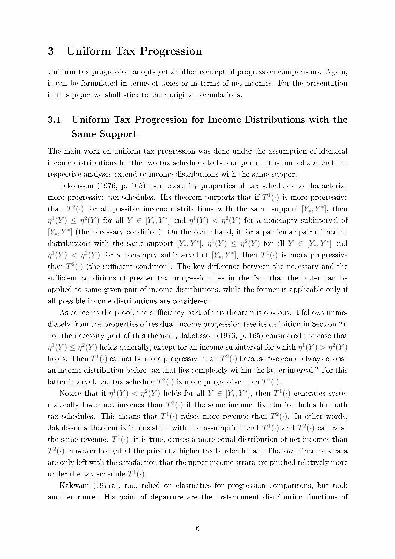
Uniform tax progression adopts yet another concept of progression comparisons. Again,

it can be formulated in terms of taxes or in terms of net incomes. For the presentation

in this paper we shall stick to their original formulations.

3.1 Uniform Tax Progression for Income Distributions with the

Same Support

The main work on uniform tax progression was done under the assumption of identical

income distributions for the two tax schedules to be compared. It is immediate that the

respective analyses extend to income distributions with the same support.

Jakobsson (1976, p. 165) used elasticity properties of tax schedules to characterize

more progressive tax schedules. His theorem purports that if T 1(·) is more progressive

than T 2(·) for all possible income distributions with the same support [Y∗, Y∗], then

η1(Y ) ≤ η2(Y ) for all Y ∈ [Y∗, Y∗] and η1(Y ) < η2(Y ) for a nonempty subinterval of

[Y∗, Y∗] (the necessary condition). On the other hand, if for a particular pair of income

distributions with the same support [Y∗, Y∗], η1(Y ) ≤ η2(Y ) for all Y ∈ [Y∗, Y

∗] and

η1(Y ) < η2(Y ) for a nonempty subinterval of [Y∗, Y∗], then T 1(·) is more progressive

than T 2(·) (the su�cient condition). The key di�erence between the necessary and the

su�cient conditions of greater tax progression lies in the fact that the latter can be

applied to some given pair of income distributions, while the former is applicable only if

all possible income distributions are considered.

As concerns the proof, the su�ciency part of this theorem is obvious; it follows imme-

diately from the properties of residual income progression (see its de�nition in Section 2).

For the necessity part of this theorem, Jakobsson (1976, p. 165) considered the case that

η1(Y ) ≤ η2(Y ) holds generally, except for an income subinterval for which η1(Y ) > η2(Y )

holds. Then T 1(·) cannot be more progressive than T 2(·) because �we could always choosean income distribution before tax that lies completely within the latter interval.� For this

latter interval, the tax schedule T 2(·) is more progressive than T 1(·).Notice that if η1(Y ) < η2(Y ) holds for all Y ∈ [Y∗, Y

∗], then T 1(·) generates syste-

matically lower net incomes than T 2(·) if the same income distribution holds for both

tax schedules. This means that T 1(·) raises more revenue than T 2(·). In other words,

Jakobsson's theorem is inconsistent with the assumption that T 1(·) and T 2(·) can raise

the same revenue. T 1(·), it is true, causes a more equal distribution of net incomes than

T 2(·), however bought at the price of a higher tax burden for all. The lower income strata

are only left with the satisfaction that the upper income strata are pinched relatively more

under the tax schedule T 1(·).Kakwani (1977a), too, relied on elasticities for progression comparisons, but took

another route. His point of departure are the �rst-moment distribution functions of

6

taxes and net incomes:

(1) FT (Y ) :=1

τ

∫ Y

Y∗

T (y)f(y)dy;

(2) FY−T (Y ) :=1

µ− τ

∫ Y

Y∗

[y − T (y)]f(y)dy.

These functions indicate the share of total tax revenue (total net income) paid (received)

by the income recipients with gross incomes less or equal to Y .

For two tax schedules Kakwani (1977a) employed the concentration curve of FT 1(Y )

relative to FT 2(Y ), and analogously for the net incomes. This relative concentration curve

is de�ned on the unit square [note that the range of both FT (Y ) and FY−T (Y ) is the unit

interval], where FT 1(Y ) is depicted on the ordinate and FT 2(Y ) on the abscissa. If this

relative concentration curve lies below the diagonal, then, except at the endpoints Y∗ and

Y ∗, FT 1(Y ) collects for all income levels Y a lower share of tax revenue than does FT 2(Y ).

Hence, FT 1(·) is more progressive than FT 2(·).The second derivative of a strictly convex (concave) function is positive (negative).

For a positive second derivative of the relative concentration curve of taxes ε1(Y ) ≥ ε2(Y )

holds, for a negative second derivative of the relative concentration curve of net incomes

η1(Y ) ≤ η2(Y ) holds. Alas, these conditions are su�cient conditions for greater tax

progression, but not necessary conditions. This results from Kakwani's con�nement to a

particular income distribution rather than to the universe of all income distributions. A

particular income distribution and two tax schedules may yield a relative concentration

curve lying wholly below the diagonal, although ε1(Y ) < ε2(Y ) holds for some subinterval

of the support of the income distribution. This applies mutatis mutandis also to net

incomes. After all, this case seems to us the more realistic one because one wants to

compare tax schedules not with respect to the universe of income distributions, but for

an empirically given pair of income distributions.

A third approach developed by Hemming and Keen (1983) relies on single crossing

conditions. According to their �ndings, T 1(·) is more progressive than T 2(·) if the net

income function Y − T 1(Y ) crosses the net income function resulting from T 2(·), viz.Y −T 2(Y ), once from below, say, at Y . In their proof, they start demonstrating that this

holds for tax schedules raising the same revenue. The intuition behind this proposition

is clear: tax progression means that the lower income strata pay relatively less than the

upper income strata under T 1(·) than under T 2(·). In other words, the lower income

strata have relatively more net income than the upper income strata under T 1(·) than

under T 2(·). By the assumption of revenue-neutral tax schedules, this translates into

absolute �gures. Due to revenue neutrality, the upper income strata have to pay exactly

the same amount of tax more under T 1(·) than under T 2(·), as the lower income strata

pay more under T 2(·) than under T 1(·). If T 1(·) and T 2(·) are not revenue neutral, then

7

the two cases have to be normalized and the argument translates into relative �gures.

This is Hemming and Keen's (1983) second proposition.

Obviously, this constitutes a su�cient condition of greater tax progression. The neces-

sary part of the proof comes from Hemming and Keen's (1983) requirement that it should

hold for all income distributions. Suppose, for instance, that there are two crossings: let

Y − T 1(Y ) cross Y − T 2(Y ) at Y > Y∗ from below and at Y , Y ∗ > Y > Y , from above.

Consider now Y , Y > Y > Y . Then there exist income distributions such that T 1(·)and T 2(·) raise the same revenue for Y ∈ [Y∗, Y ) and raise the same revenue (possibly

di�erent from the �rst interval) for Y ∈ [Y , Y ∗]. Then T 1(·) is more progressive than

T 2(·) on the income interval [Y∗, Y ) and less progressive on [Y , Y ∗]. Hence, the necessary

part of the proof requires that the single-crossing condition should hold for the universe

of income distributions.

The relationship between Kakwani's (1977a) elasticity condition and Hemming and

Keen's (1983) single-crossing condition is the following: obviously

(3) lnY − T 1(Y )

Y − T 2(Y )= ln[Y − T 1(Y )]− ln[Y − T 2(Y )].

Di�erentiating this with respect to Y , multiplying the right-hand side by YY, re-arranging

and using the de�nition for η(Y ) yields

(4)d

dY{ln[Y − T 1(Y )]− ln[Y − T 2(Y )]} =

η1(Y )− η2(Y )

Y.

Applying an exponential transformation on Equation (3) and substituting the integral of

Equation (4) yields

(5)Y − T 1(Y )

Y − T 2(Y )= e

∫ YY

η1(y)−η2(y)y

dy

for Y ≤ Y ≤ Y ∗, where Y denotes the income at which the net income curves cross.

When η1(Y ) ≤ η2(Y ) for all Y > Y and the inequality sign is strict for some nonempty

interval of (Y , Y ∗], then [Y −T 1(Y )] < [Y −T 2(Y )] for all y ∈ (Y , Y ∗]. In other words, the

single-crossing condition holds. Hence, the condition η1(Y ) ≤ η2(Y ) for all Y ∈ [Y∗, Y∗]

is su�cient for the single-crossing condition to hold. Conversely, when the single-crossing

condition holds, this does not imply that η1(Y ) ≤ η2(Y ) for all Y ∈ [Y∗, Y∗]. η1(Y ) >

η2(Y ) may well hold for a subinterval of [Y∗, Y ), or for a subinterval of (Y , Y ∗], while

leaving the integral term in equation (5) negative.

Uniform measures of tax progression for identical income distributions, or, more gen-

erally, for income distributions with the same support, have several drawbacks. First,

by de�nition, they are only applicable for comparing tax schedules in situations with

the same income distributions or at least the same support of the income distributions.

Hence, they cannot be used for international or intertemporal comparisons of tax pro-

gression which are typically associated with di�erent income distributions and di�erent

8

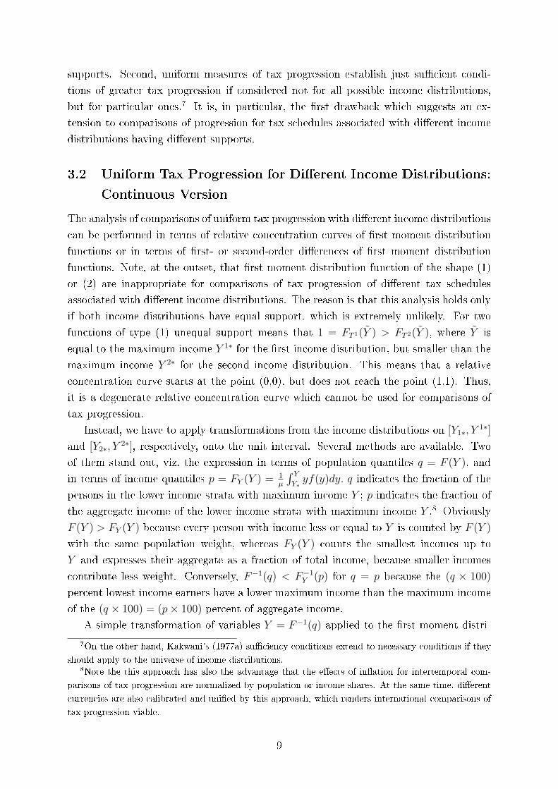
supports. Second, uniform measures of tax progression establish just su�cient condi-

tions of greater tax progression if considered not for all possible income distributions,

but for particular ones.7 It is, in particular, the �rst drawback which suggests an ex-

tension to comparisons of progression for tax schedules associated with di�erent income

distributions having di�erent supports.

3.2 Uniform Tax Progression for Di�erent Income Distributions:

Continuous Version

The analysis of comparisons of uniform tax progression with di�erent income distributions

can be performed in terms of relative concentration curves of �rst moment distribution

functions or in terms of �rst- or second-order di�erences of �rst moment distribution

functions. Note, at the outset, that �rst moment distribution function of the shape (1)

or (2) are inappropriate for comparisons of tax progression of di�erent tax schedules

associated with di�erent income distributions. The reason is that this analysis holds only

if both income distributions have equal support, which is extremely unlikely. For two

functions of type (1) unequal support means that 1 = FT 1(Y ) > FT 2(Y ), where Y is

equal to the maximum income Y 1∗ for the �rst income distribution, but smaller than the

maximum income Y 2∗ for the second income distribution. This means that a relative

concentration curve starts at the point (0,0), but does not reach the point (1,1). Thus,

it is a degenerate relative concentration curve which cannot be used for comparisons of

tax progression.

Instead, we have to apply transformations from the income distributions on [Y1∗, Y1∗]

and [Y2∗, Y2∗], respectively, onto the unit interval. Several methods are available. Two

of them stand out, viz. the expression in terms of population quantiles q = F (Y ), and

in terms of income quantiles p = FY (Y ) = 1µ

∫ YY∗yf(y)dy. q indicates the fraction of the

persons in the lower income strata with maximum income Y ; p indicates the fraction of

the aggregate income of the lower income strata with maximum income Y .8 Obviously

F (Y ) > FY (Y ) because every person with income less or equal to Y is counted by F (Y )

with the same population weight, whereas FY (Y ) counts the smallest incomes up to

Y and expresses their aggregate as a fraction of total income, because smaller incomes

contribute less weight. Conversely, F−1(q) < F−1Y (p) for q = p because the (q × 100)

percent lowest income earners have a lower maximum income than the maximum income

of the (q × 100) = (p× 100) percent of aggregate income.

A simple transformation of variables Y = F−1(q) applied to the �rst moment distri-

7On the other hand, Kakwani's (1977a) su�ciency conditions extend to necessary conditions if they

should apply to the universe of income distributions.8Note the this approach has also the advantage that the e�ects of in�ation for intertemporal com-

parisons of tax progression are normalized by population or income shares. At the same time, di�erent

currencies are also calibrated and uni�ed by this approach, which renders international comparisons of

tax progression viable.

9

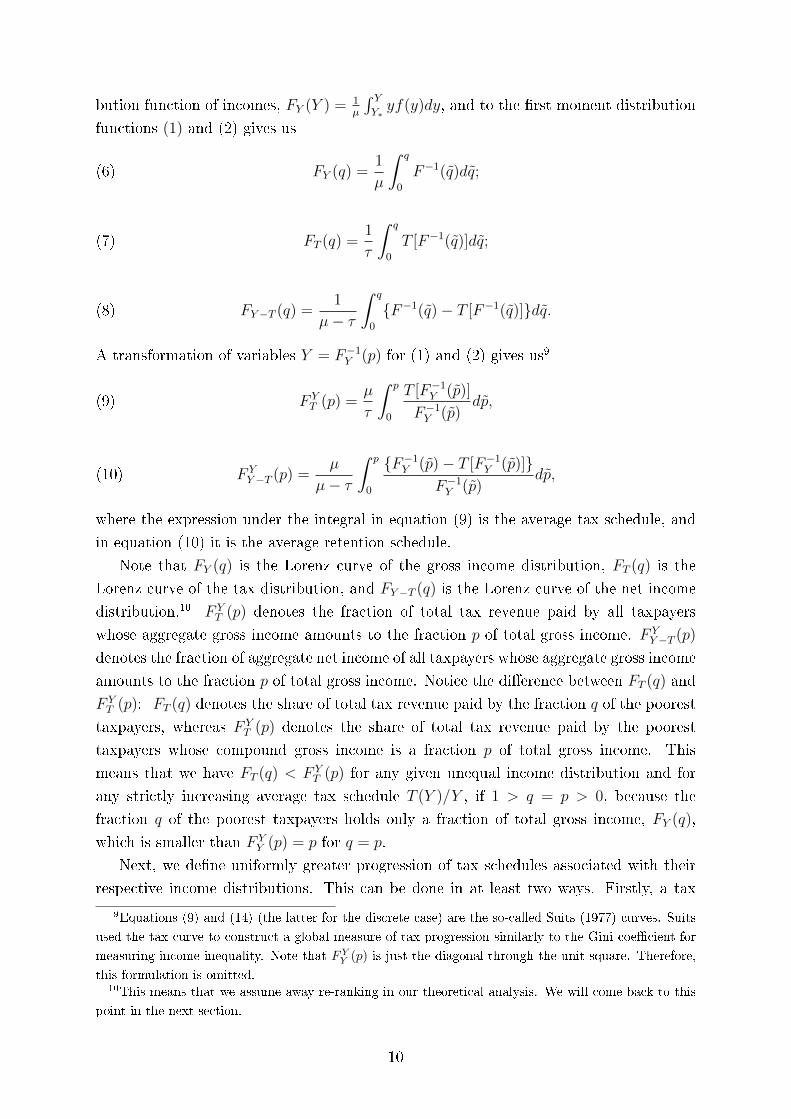
bution function of incomes, FY (Y ) = 1µ

∫ YY∗yf(y)dy, and to the �rst moment distribution

functions (1) and (2) gives us

(6) FY (q) =1

µ

∫ q

0

F−1(q)dq;

(7) FT (q) =1

τ

∫ q

0

T [F−1(q)]dq;

(8) FY−T (q) =1

µ− τ

∫ q

0

{F−1(q)− T [F−1(q)]}dq.

A transformation of variables Y = F−1Y (p) for (1) and (2) gives us9

(9) F YT (p) =

µ

τ

∫ p

0

T [F−1Y (p)]

F−1Y (p)dp,

(10) F YY−T (p) =

µ

µ− τ

∫ p

0

{F−1Y (p)− T [F−1Y (p)]}F−1Y (p)

dp,

where the expression under the integral in equation (9) is the average tax schedule, and

in equation (10) it is the average retention schedule.

Note that FY (q) is the Lorenz curve of the gross income distribution, FT (q) is the

Lorenz curve of the tax distribution, and FY−T (q) is the Lorenz curve of the net income

distribution.10 F YT (p) denotes the fraction of total tax revenue paid by all taxpayers

whose aggregate gross income amounts to the fraction p of total gross income. F YY−T (p)

denotes the fraction of aggregate net income of all taxpayers whose aggregate gross income

amounts to the fraction p of total gross income. Notice the di�erence between FT (q) and

F YT (p): FT (q) denotes the share of total tax revenue paid by the fraction q of the poorest

taxpayers, whereas F YT (p) denotes the share of total tax revenue paid by the poorest

taxpayers whose compound gross income is a fraction p of total gross income. This

means that we have FT (q) < F YT (p) for any given unequal income distribution and for

any strictly increasing average tax schedule T (Y )/Y , if 1 > q = p > 0, because the

fraction q of the poorest taxpayers holds only a fraction of total gross income, FY (q),

which is smaller than F YY (p) = p for q = p.

Next, we de�ne uniformly greater progression of tax schedules associated with their

respective income distributions. This can be done in at least two ways. Firstly, a tax

9Equations (9) and (14) (the latter for the discrete case) are the so-called Suits (1977) curves. Suits

used the tax curve to construct a global measure of tax progression similarly to the Gini coe�cient for

measuring income inequality. Note that FYY (p) is just the diagonal through the unit square. Therefore,

this formulation is omitted.10This means that we assume away re-ranking in our theoretical analysis. We will come back to this

point in the next section.

10

Figure 1: Construction of a relative concentration curve from Lorenz curves for taxes

schedule T 1 can be de�ned to be uniformly more progressive than T 2 whenever the

concentration curve of FT 1 relative to FT 2 does not cross the diagonal of the unit square

except at the endpoints (0,0) and (1,1). To illustrate, we focus on the case of entering FT 1

on the ordinate and FT 2 on the abscissa, and on the half-space of the unit square below the

diagonal. Other arrangements are immediate. This means that for the same fractions q or

p as applied to the two income distributions,11 T 1 collects a smaller fraction of aggregate

taxes from smaller incomes than does T 2. A su�cient condition for the concentration

curve of FT 1 relative to FT 2 to lie wholly below the diagonal of the unit square is that it

is strictly convex.12 Figure 1 illustrates this case in terms of q.

Alas, the convexity (or concavity) condition is not a necessary condition for greater

tax progression. When comparing two situations, then there may well occur cases such

that convexity or concavity of the relative concentration curve is violated without its

crossing the diagonal within the unit square. Figure 2 illustrates.

11It can also be performed in terms of Y but this would require that both income distributions involved

have equal support; see Seidl (1994, pp. 347-9).12Equivalently, one can require that the slope of a relative concentration curve be less than one below

a unique value of its argument and greater than one thereafter. Whereas this is equivalent to strict

convexity for the case of relative concentration curves, strict convexity produces the more intuitive and

precise formulations of the su�cient conditions.

11

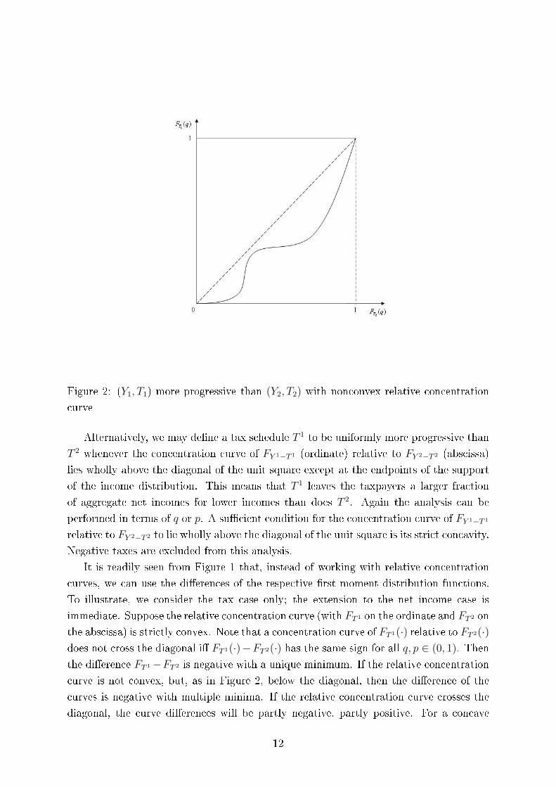
Figure 2: (Y1, T1) more progressive than (Y2, T2) with nonconvex relative concentration

curve

Alternatively, we may de�ne a tax schedule T 1 to be uniformly more progressive than

T 2 whenever the concentration curve of FY 1−T 1 (ordinate) relative to FY 2−T 2 (abscissa)

lies wholly above the diagonal of the unit square except at the endpoints of the support

of the income distribution. This means that T 1 leaves the taxpayers a larger fraction

of aggregate net incomes for lower incomes than does T 2. Again the analysis can be

performed in terms of q or p. A su�cient condition for the concentration curve of FY 1−T 1

relative to FY 2−T 2 to lie wholly above the diagonal of the unit square is its strict concavity.

Negative taxes are excluded from this analysis.

It is readily seen from Figure 1 that, instead of working with relative concentration

curves, we can use the di�erences of the respective �rst moment distribution functions.

To illustrate, we consider the tax case only; the extension to the net income case is

immediate. Suppose the relative concentration curve (with FT 1 on the ordinate and FT 2 on

the abscissa) is strictly convex. Note that a concentration curve of FT 1(·) relative to FT 2(·)does not cross the diagonal i� FT 1(·)−FT 2(·) has the same sign for all q, p ∈ (0, 1). Then

the di�erence FT 1−FT 2 is negative with a unique minimum. If the relative concentration

curve is not convex, but, as in Figure 2, below the diagonal, then the di�erence of the

curves is negative with multiple minima. If the relative concentration curve crosses the

diagonal, the curve di�erences will be partly negative, partly positive. For a concave

12

relative concentration curve, the curve di�erences are positive, single peaked for a strictly

concave relative concentration curve, and multiple peaked for a non-concave relative

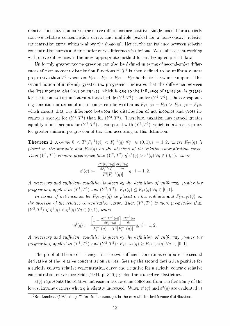
concentration curve which is above the diagonal. Hence, the equivalence between relative

concentration curves and �rst-order curve di�erences is obvious. We shall see that working

with curve di�erences is the more appropriate method for analyzing empirical data.

Uniformly greater tax progression can also be de�ned in terms of second-order di�er-

ences of �rst moment distribution functions.13 T 1 is then de�ned to be uniformly more

progressive than T 2 whenever FY 1 − FT 1 > FY 2 − FT 2 holds for the whole support. This

second notion of uniformly greater tax progression indicates that the di�erence between

the �rst moment distribution curves, which is due to the in�uence of taxation, is greater

for the income-distribution-cum-tax-schedule (Y 1, T 1) than for (Y 2, T 2). The correspond-

ing condition in terms of net incomes can be written as FY 1−T 1 − FY 1 > FY 2−T 2 − FY 2 ,

which means that the di�erence between the distribution of net incomes and gross in-

comes is greater for (Y 1, T 1) than for (Y 2, T 2). Therefore, taxation has caused greater

equality of net incomes for (Y 1, T 1) as compared with (Y 2, T 2), which is taken as a proxy

for greater uniform progression of taxation according to this de�nition.

Theorem 1 Assume 0 < T i[F−1i (q)] < F−1i (q) ∀q ∈ (0, 1), i = 1, 2, where FT 1(q) is

placed on the ordinate and FT 2(q) on the abscissa of the relative concentration curve.

Then (Y 1, T 1) is more progressive than (Y 2, T 2) if ε1(q) > ε2(q) ∀q ∈ (0, 1), where

εi(q) :=

dT i[F−1i (q)]

dF−1i (q)

dF−1i (q)

dq

T i[F−1i (q)]q, i = 1, 2.

A necessary and su�cient condition is given by the de�nition of uniformly greater tax

progression, applied to (Y 1, T 1) and (Y 2, T 2): FT 1(q) ≤ FT 2(q) ∀q ∈ [0, 1].

In terms of net incomes let FY 1−T 1(q) be placed on the ordinate and FY 2−T 2(q) on

the abscissa of the relative concentration curve. Then (Y 1, T 1) is more progressive than

(Y 2, T 2) if η1(q) < η2(q) ∀q ∈ (0, 1), where

ηi(q) :=

[1− dT i[F−1

i (q)]

dF−1i (q)

]dF−1i (q)

dq

F−1i (q)− T i[F−1i (q)]q, i = 1, 2.

A necessary and su�cient condition is given by the de�nition of uniformly greater tax

progression, applied to (Y 1, T 1) and (Y 2, T 2): FY 1−T 1(q) ≥ FY 2−T 2(q) ∀q ∈ [0, 1].

The proof of Theorem 1 is easy: for the two su�cient conditions compute the second

derivative of the relative concentration curves. Setting the second derivative positive for

a strictly convex relative concentration curve and negative for a strictly concave relative

concentration curve (see Seidl (1994, p. 349)) yields the respective elasticities.

ε(q) represents the relative increase in tax revenue collected from the fraction q of the

lowest income earners when q is slightly increased. When ε1(q) and ε2(q) are evaluated at

13See Lambert (1989, chap. 7) for similar concepts in the case of identical income distributions.

13

the same value of q, for di�erent income distributions this means that they are evaluated

at di�erent income levels and/or in di�erent monetary units. Assume, for instance, that

we have F−11 (q) = Y 1 and F−12 (q) = Y 2. Then we are actually comparing

ε1(q) =dT 1(Y 1)/dY 1

T 1(Y 1)f1(Y 1)q and ε2(q) =

dT 2(Y 2))/dY 2

T 2(Y 2)f2(Y 2)q,

where we have usually Y 1 6= Y 2, even if we are comparing tax schedules de�ned for

the same monetary unit. Notice the tendency of a more unequal income distribution to

make the tax system more progressive, because a smaller Y is associated with q, which

means that there is not much income concentrated in the fraction q of the poorest income

earners. Therefore not much tax revenue can be extracted from the lower income strata.

Note that these elasticities are not only cast in terms of tax or net income schedules,

but contain elements of both the tax schedules and the income distributions. They are

algebraic conditions but, alas, are only su�cient and not necessary conditions. The

respective de�nitions are trivial necessary and su�cient conditions which are helpful for

empirical analyses.14

Theorem 2 Assume 0 < T i[F−1Y i

(p)] < F−1Y i

(p) ∀p ∈ (0, 1), i = 1, 2, where F YT 1(p) is

placed on the ordinate and F YT 2(p) on the abscissa of the relative concentration curve. Then

(Y 1, T 1) is more progressive than (Y 2, T 2) if ε1(p) − χ1(p) > ε2(p) − χ2(p) ∀p ∈ (0, 1),

where

εi(p) :=

dT i[F−1Yi

(p)]

dF−1

Y i(p)

dF−1

Y i(p)

dp

T i[F−1Y i

(p)]p, and χi(p) :=

dF−1Y i

(p)

dp

p

F−1Y i

i = 1, 2.

A necessary and su�cient condition is given by the de�nition of uniformly greater tax

progression, applied to (Y 1, T 1) and (Y 2, T 2): FT 1(p) ≤ FT 2(p) ∀p ∈ [0, 1].

In terms of net incomes, let F YY 1−T 1(p) be placed on the ordinate and F Y

Y 2−T 2(p) on

the abscissa of the relative concentration curve. Then (Y 1, T 1) is more progressive than

(Y 2, T 2) if η1(p)− χ1(p) < η2(p)− χ2(p) ∀p ∈ (0, 1), where

ηi(p) :=

[1−

dT i[F−1Yi

(p)]

dF−1

Y i(p)

]dF−1Yi

(p)

dp

F−1Yi(p)− Ti[F−1Yi

(p)]p, and χi(p) :=

dF−1Y i

(p)

dp

p

F−1Y i

i = 1, 2.

A necessary and su�cient condition is given by the de�nition of uniformly greater tax

progression, applied to (Y 1, T 1) and (Y 2, T 2): FY 1−T 1(p) ≥ FY 2−T 2(p) ∀p ∈ [0, 1].

Theorem 2 again contains two su�cient and two trivial necessary and su�cient con-

ditions. What we have reasoned after Theorem 1 applies, mutatis mutandis, also for

14Although having a necessary and su�cient condition for their analysis in terms of deformed income

distributions, viz. isoelasticity of the deformation functions to warrant independence of the baseline dis-

tribution, Dardanoni and Lambert (2002, p. 106) had to concede that isoelasticity is a rather demanding

14

Theorem 2. The only di�erence is that now the comparison of progression is made in

terms of shares of aggregate income instead of in income shares of population strata.

As concerns the su�cient conditions, ε(p) [η(p)] denotes the tax [residual income]

elasticity with respect to p, and χ(p) denotes the elasticity of the inverse �rst moment

distribution function with respect to p, which captures the in�uence of the income dis-

tribution evaluated at p. The proof of Theorem 2 is a complete analogue of that of

Theorem 1, if applied to relative concentration curves in terms of income shares. When

ε1(p) − χ1(p) and ε2(p) − χ2(p) are evaluated at the same value of p, this means that

di�erent Yi's are involved.

The next theorem analyzes greater progression in terms of second-order di�erences of

�rst moment distribution functions.

Theorem 3 Assume 0 < T i[F−1i (q)] < F−1i (q) ∀ q ∈ (0, 1), i = 1, 2. Then FY 1(q) −FT 1(q) > FY 2(q)− FT 2(q) > 0 ∀ q ∈ (0, 1), if both ε1(q) ≥ ε2(q) and Ψ1(q) ≤ Ψ2(q) ∀q ∈(0, 1), where at least one of the two inequality signs has to be strict. Notice that εi(q),

i = 1, 2, is de�ned as in Theorem 1, and Ψi(q) :=dF−1i

(q)

dq

F−1i (q)

q, i = 1, 2, denotes the elasticity

of the inverse distribution function.

A necessary and su�cient condition is given by the de�nition of uniformly greater tax

progression, applied to (Y 1, T 1) and (Y 2, T 2): FY 1(q) − FT 1(q) ≥ FY 2(q) − FT 2(q) >

0 ∀ q ∈ (0, 1).

Moreover, FY 1(q) − FY 1−T 1(q) < FY 2(q) − FY 2−T 2(q) < 0 ∀ q ∈ (0, 1) if both η1(q) ≤η2(q) and Ψ1(q) ≥ Ψ2(q) ∀ q ∈ (0, 1), where at least one of the two inequality signs has

to be strict. Notice that ηi(q), i = 1, 2, is de�ned as in Theorem 1.

A necessary and su�cient condition is given by the de�nition of uniformly greater tax

progression, applied to (Y 1, T 1) and (Y 2, T 2): FY 1(q)−FY 1−T 1(q) ≤ FY 2(q)−FY 2−T 2(q) <

0 ∀ q ∈ (0, 1).

The proof of Theorem 3 is more involved than the proof of Theorem 1 (see Seidl

(1994, pp. 352-3)). Note that the algebraic conditions are only su�cient conditions.

They contain in their �rst components elements of both the tax schedule and the income

distribution, while their second components refer to the income distributions only. These

latter components serve the role of a calibration device to warrant that the tax distri-

butions are not triggered by great discrepancies in the distributions of gross incomes.

The necessary and su�cient conditions are again elementary; they are very helpful for

empirical analyses.

Theorem 3 concerns comparisons between di�erences of cumulative curves of gross

incomes and taxes and comparisons between di�erences of cumulative curves of net in-

comes and gross incomes. If FY 1(q) is more diminished by subtraction of the tax curve,

viz. FT 1(q), than FY 2(q) is by FT 2(q) for all q, 0 ≤ q ≤ 1, then (Y 1, T 1) is more progressive

condition which will hardly be met in the real world. (For this approach see also Footnote 1.) Hence, com-

15

than (Y 2, T 2). If FY 1−T 1(q) is more diminished by subtraction of FY 1(q) than FY 2−T 2(q)

is by FY 2(q) for all q, 0 ≤ q ≤ 1, then (Y 1, T 1) is more progressive than (Y 2, T 2).

Note that dominance relations of concentrations curves are subrelations of appropriate

global inequality measures; of course, the converse does not hold. In this paper, we do

not dwell on that; for more details see Seidl (1994, pp. 359-60).

3.3 Uniform Tax Progression for Di�erent Income Distributions:

Discrete Version

So far empirical comparisons of tax progression have not been made for the uniform

measures of tax progression in terms of q or p that allow to compare progression for

di�erent income distributions in di�erent countries or di�erent time periods in the same

countries. We investigate the theory developed in the preceding section using the data

from the Luxembourg Income Study (LIS). As the LIS data are micro data, we have to

re-state all de�nitions and curves in discrete terms.

As we analyze comparisons of progression of direct taxes on the one hand, and direct

taxes plus payroll taxes (mainly employees' share of social security contributions) on

the other, we have to introduce the respective notation. We use Y = [Y1, Y2, . . . , Yn]

to denote a distribution of pre-tax or gross incomes arranged in nondecreasing order,

T = [T1, T2, . . . , Tn] to denote the distribution of the associated direct taxes, and S =

[S1, S2, . . . , Sn] to denote the distribution of direct taxes plus payroll taxes. µ, τ , and

ζ denote mean pre-tax or gross income, mean direct taxes, and mean direct taxes plus

payroll taxes, respectively. For generic references we will continue to use the terms

gross and net incomes. When respective discriminations are needed, the terms pre-tax

and post-tax incomes will be used for direct taxes only, and gross and net incomes for

analyses of direct taxes plus payroll taxes.

Let (Y, T ) denote the income-distribution-cum-tax-schedule for some country or some

time period within a country. Let us also de�ne the discrete equivalents of the �rst

moment distribution functions in terms of point coordinates with the �rst entry being

the ordinate, and the second entry being the abscissa of the respective points. For ease

of demonstration, T and τ are used as proxies also representing (T + S) and (τ + ζ):

(11) FY (qk) :=

∑ki=0 Yinµ

, qk =k

n, k = 0, . . . , n;

(12) FT (qk) :=

∑ki=0 Tinτ

, qk =k

n, k = 0, . . . , n;

(13) FY−T (qk) :=

∑ki=0(Yi − Ti)n(µ− τ)

, qk =k

n, k = 0, . . . , n;

parison of tax progression �becomes an empirical question�, which is another impetus for our present work.

16

(14) F YT (pk) :=

∑ki=0 Tinτ

, pk =

∑ki=0 Yinµ

k = 0, . . . , n;

(15) F YY−T (pk) :=

∑ki=0(Yi − Ti)n(µ− τ)

, pk =

∑ki=0 Yinµ

k = 0, . . . , n.

In formulae (11) to (15), we set Y0 and T0 equal to zero, which allows us to include

the origin into our curves15. Strictly speaking, both the right-hand side and the left-hand

side of (11) to (15) are functions of k. Hence we consider the range of the right-hand-side

function as the domain of the left-hand-side function, which gives us the discrete versions

of the �rst-moment distribution functions. For all curves in terms of q we use the ranking

according to gross incomes, as we have to apply that necessarily also for the curves in

terms of p. Here, (11) denotes a discrete equivalent of the Lorenz income curve, (12), and

(13) denote the discrete equivalents of the concentration curves of taxes and net incomes,

respectively. (14) and (15) denote the discrete equivalents of the concentration curves

of taxes and net incomes for the income shares pjk. These mappings are just generic; of

course, di�erent situations (Y 1, T 1) and (Y 2, T 2) have di�erent components and di�erent

numbers of income recipients.16

Concentration curves may be di�erent from Lorenz curves because of re-ranking phe-

nomena. Hence, before proceeding further, we have to dwell on the re-ranking prob-

lem which we assumed away for our theoretical analyses, but which haunts all empir-

ical analyses of distributional problems. For theoretical analyses, the assumption of

co-monotonicity of gross incomes, taxes, payroll taxes, and net incomes is self-evident:

higher gross incomes should imply higher taxes, higher payroll taxes, and higher net in-

comes. This means that the ordering of gross incomes coincides with the orderings of

taxes, payroll taxes, and net incomes. Hence, only one ordering applies to all designs and

we can work with Lorenz curves (or their discrete-case equivalents) throughout. How-

ever, in the world of empirical data, re-ranking is ubiquitous. Due to di�erent family

structures, di�erent tax allowances, di�erent income compositions, and di�erent transfer

incomes, households with higher incomes may end up with smaller taxes or, else, with

smaller net incomes than households with smaller gross incomes.

Hence, re-ranking opens up Pandora's box of possible other orderings. For instance,

for expression (12) we can arrange the entries in nondecreasing order of the taxes instead

of arranging them according to the order of their associated gross incomes. In (13), net

incomes can be arranged in nondecreasing order instead of arranging them according

to their associated gross incomes. Then we could work with Lorenz curves throughout

instead of using concentration curves. Indeed, in the presence of re-ranking, concentration

curves would be closer to the diagonal than Lorenz curves, or may even cross the diagonal.

15Recall that we exclude negative incomes and taxes in our empirical analysis.16Note that for the discrete version we continue to use superscripts to refer to the two di�erent vectors

of taxes and incomes, each representing the situation as a whole, while subscripts are used for vector

17

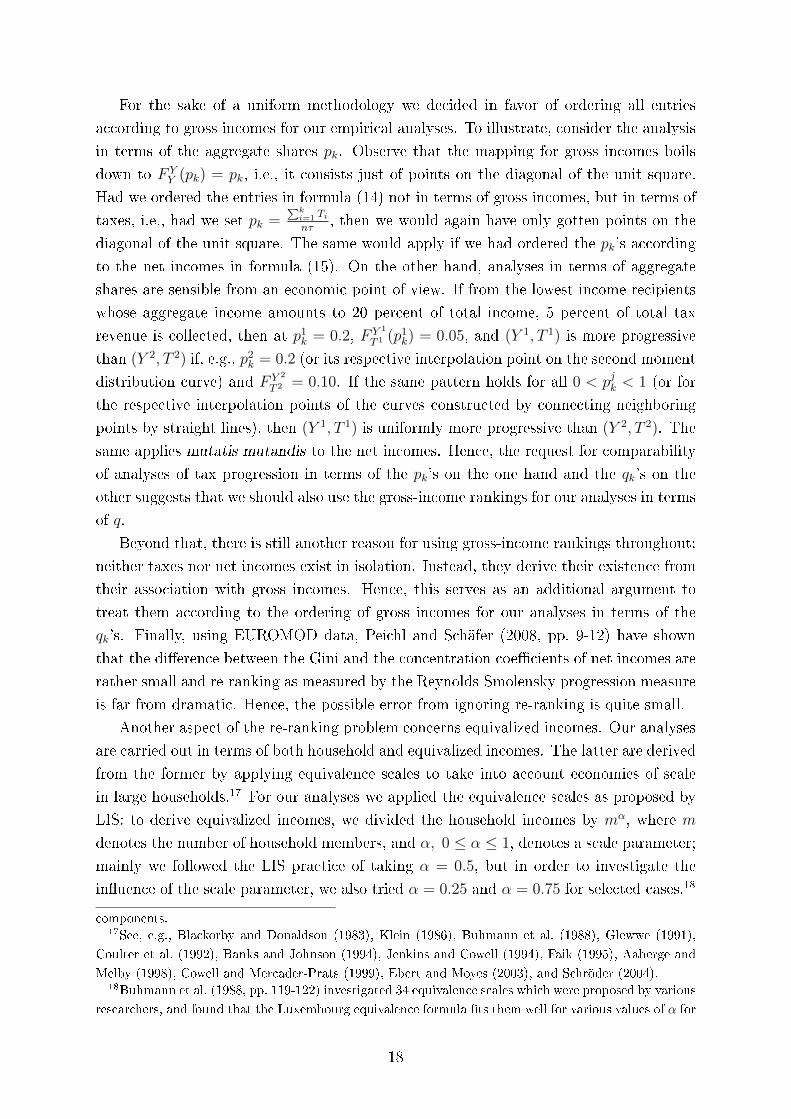
For the sake of a uniform methodology we decided in favor of ordering all entries

according to gross incomes for our empirical analyses. To illustrate, consider the analysis

in terms of the aggregate shares pk. Observe that the mapping for gross incomes boils

down to F YY (pk) = pk, i.e., it consists just of points on the diagonal of the unit square.

Had we ordered the entries in formula (14) not in terms of gross incomes, but in terms of

taxes, i.e., had we set pk =∑ki=1 Tinτ

, then we would again have only gotten points on the

diagonal of the unit square. The same would apply if we had ordered the pk's according

to the net incomes in formula (15). On the other hand, analyses in terms of aggregate

shares are sensible from an economic point of view. If from the lowest income recipients

whose aggregate income amounts to 20 percent of total income, 5 percent of total tax

revenue is collected, then at p1k = 0.2, F Y 1

T 1 (p1k) = 0.05, and (Y 1, T 1) is more progressive

than (Y 2, T 2) if, e.g., p2k = 0.2 (or its respective interpolation point on the second moment

distribution curve) and F Y 2

T 2 = 0.10. If the same pattern holds for all 0 < pjk < 1 (or for

the respective interpolation points of the curves constructed by connecting neighboring

points by straight lines), then (Y 1, T 1) is uniformly more progressive than (Y 2, T 2). The

same applies mutatis mutandis to the net incomes. Hence, the request for comparability

of analyses of tax progression in terms of the pk's on the one hand and the qk's on the

other suggests that we should also use the gross-income rankings for our analyses in terms

of q.

Beyond that, there is still another reason for using gross-income rankings throughout:

neither taxes nor net incomes exist in isolation. Instead, they derive their existence from

their association with gross incomes. Hence, this serves as an additional argument to

treat them according to the ordering of gross incomes for our analyses in terms of the

qk's. Finally, using EUROMOD data, Peichl and Schäfer (2008, pp. 9-12) have shown

that the di�erence between the Gini and the concentration coe�cients of net incomes are

rather small and re-ranking as measured by the Reynolds-Smolensky progression measure

is far from dramatic. Hence, the possible error from ignoring re-ranking is quite small.

Another aspect of the re-ranking problem concerns equivalized incomes. Our analyses

are carried out in terms of both household and equivalized incomes. The latter are derived

from the former by applying equivalence scales to take into account economies of scale

in large households.17 For our analyses we applied the equivalence scales as proposed by

LIS: to derive equivalized incomes, we divided the household incomes by mα, where m

denotes the number of household members, and α, 0 ≤ α ≤ 1, denotes a scale parameter;

mainly we followed the LIS practice of taking α = 0.5, but in order to investigate the

in�uence of the scale parameter, we also tried α = 0.25 and α = 0.75 for selected cases.18

components.17See, e.g., Blackorby and Donaldson (1983), Klein (1986), Buhmann et al. (1988), Glewwe (1991),

Coulter et al. (1992), Banks and Johnson (1994), Jenkins and Cowell (1994), Faik (1995), Aaberge and

Melby (1998), Cowell and Mercader-Prats (1999), Ebert and Moyes (2003), and Schröder (2004).18Buhmann et al. (1988, pp. 119-122) investigated 34 equivalence scales which were proposed by various

researchers, and found that the Luxembourg equivalence formula �ts them well for various values of α for

18

To illustrate, consider an income distribution comprising two households: [1000,2500].

Suppose that the �rst one is a single-person household, while the second one is a four-

person household. Then, if we take α = 0.5, the equivalized income distribution becomes

[1000,1250,1250,1250,1250]; however, taking α = 0.75 gives us the equivalized income

distribution [884,884,884,884,1000]. Hence, both the household structure19 and the choice

of the scale parameter determine the shape of the equivalized income distribution. In our

analysis, equivalized incomes were always arranged in nondecreasing order of equivalized

gross incomes.

After the digression on re-ranking, let us return to the concepts of uniformly more

progressive tax schedules. Recall that we de�ned (Y 1, T 1) to be more progressive than

(Y 2, T 2) if the tax schedule T 1 associated with the income distribution Y 1 collects for all

values of q or p no greater fraction of taxes than does tax schedule T 2 associated with the

income distribution Y 2. Alternatively, we de�ned greater progression of (Y 1, T 1) than

(Y 2, T 2) if (Y 1, T 1) leaves the taxpayers for all q or p no less a fraction of post-tax net

incomes than does (Y 2, T 2). Finally, we de�ned greater progression if the di�erence of

the cumulative curves of gross incomes and taxes for (Y 1, T 1) is not smaller than the

di�erence of the cumulative curves of gross incomes and taxes for (Y 2, T 2) for all q, or

when the di�erence of the cumulative curves of gross and net incomes of (Y 1, T 1) is not

greater than the di�erence of the cumulative curves of gross incomes and taxes of (Y 2, T 2)

for all q.20

For the continuous analyses we expressed the �rst two concepts in terms of relative

concentration curves, and the second two in terms of second-order curve di�erences. More

progression is present if the relative concentration curve does not cut the diagonal within

the unit square, or if the second-order curve di�erences do not cut the abscissa within

the unit interval. For the discrete analysis, it is more convenient to use curve di�erences

quite generally.21 As the respective �curves� in the discrete case consist of �nitely many

four representative groups of proposed equivalence scales. Buhmann et al. (1988, p. 128) also observed

that income inequality �rst decreases and then increases as α increases, viz. inequality is an U-shaped

function of α; poverty decreases as α increases (p. 132). For more elaborate work see Coulter et al.

(1992), Banks and Johnson (1994), Jenkins and Cowell (1994), Faik (1995), and Cowell and Mercader-

Prats (1999).19Buhmann et al. (1988, p. 127) argue that equivalence scales have greater e�ect in case of di�erent

household structures associated with the actual income distributions to be compared; greater households,

in particular, in�uence the results. Peichl et al. (2009a,b) observed that part of the increase in income

inequality in Germany in terms of equivalized incomes is due to the trend in the direction of smaller

households in the last decades.20See also p. 12. Concerning the de�nitions in terms of p. see Footnote 9, which applies to the discrete

case as well.21The case of a relative concentration curve being below (or above) the diagonal in the interior of

the unit square is equivalent to a positive (negative) di�erence of the generating curves within the unit

interval. Recall that a concentration curve of FT 1(·) relative to FT 2(·) does not cross the diagonal i�

FT 1(·) − FT 2(·) has the same sign for all q, p ∈ (0, 1). The proof is trivial and therefore omitted. Note

that this applies analogously also to net incomes.

19

points, we have to con�ne ourselves to the comparison of these points. In the general

case, as de�ned in formulae (11) to (15), we encounter the di�culty that the qk's and

the pk's need not coincide for (Y 1, T 1) and (Y 2, T 2), so that we may have k1's for which

there are no equal k2's, and vice versa. This can be handled in a more tedious way by

comparing q1k with the equivalent point on the interpolation segment on the second curve.

For reasons to be explained in Sections 4.1 and 4.2 we used grouped data with the same

number of quantiles. Before that, we explain our measures of comparisons of progression

in terms of individual data.

For the sake of uni�ed representation we have arranged all de�nitions of greater pro-

gression in such a way that progression dominance is expressed as nonnegative curve

di�erences and being progression dominated as nonpositive curve di�erences. Hence, we

have:

De�nition 1 (Y 1, T 1) is more [less] progressive than (Y 2, T 2) i� FT 2(qk) − FT 1(qk) is

nonnegative [nonpositive] for all qk, 0 ≤ qk ≤ 1.

De�nition 2 (Y 1, T 1) is more [less] progressive than (Y 2, T 2) i� F YT 2(pk) − F Y

T 1(pk) is

nonnegative [nonpositive] for all pk, 0 ≤ pk ≤ 1.

De�nition 3 (Y 1, T 1) is more [less] progressive than (Y 2, T 2) i� FY 1−T 1(qk)−FY 2−T 2(qk)

is nonnegative [nonpositive] for all qk, 0 ≤ qk ≤ 1.

De�nition 4 (Y 1, T 1) is more [less] progressive than (Y 2, T 2) i� F YY 1−T 1(pk)−F Y

Y 2−T 2(pk)

is nonnegative [nonpositive] for all pk, 0 ≤ pk ≤ 1.

De�nition 5 (Y 1, T 1) is more [less] progressive than (Y 2, T 2) i� [FY 1(qk) − FY 2(qk)] −[FT 1(qk)− FT 2(qk)] is nonnegative [nonpositive] for all qk, 0 ≤ qk ≤ 1.

De�nition 6 (Y 1, T 1) is more [less] progressive than (Y 2, T 2) i� [FY 1−T 1(qk)−FY 2−T 2(qk)]−[FY 1(qk)− FY 2(qk)] is nonnegative [nonpositive] for all qk, 0 ≤ qk ≤ 1.

Obviously, De�nition 1 matches the necessary and su�cient conditions of the �rst

part of Theorem 1. De�nition 2 matches the necessary and su�cient condition of the

�rst part of Theorem 2. De�nition 3 matches the necessary and su�cient condition of the

second part of Theorem 1. De�nition 4 matches the necessary and su�cient condition of

the second part of Theorem 2. De�nition 5 matches the necessary and su�cient condition

of the �rst part of Theorem 3. Note that De�nition 5 comes from the formulation that

(Y 1, T 1) is more [less] progressive than (Y 2, T 2) i� [FY 1(qk)−FT 1(qk)] ≥ [FY 2(qk)−FT 2(qk)]

[≤ for less progressive] for all qk, 0 ≤ qk ≤ 1. De�nition 6 matches the necessary and

su�cient condition of the second part of Theorem 3. Note that De�nition 6 comes from

the formulation that (Y 1, T 1) is more [less] progressive than (Y 2, T 2) i� [FY 1−T 1(qk) −FY 1(qk)] ≥ [FY 2−T 2(qk)− FY 2(qk)] [≤ for less progressive] for all qk, 0 ≤ qk ≤ 1.

20

3.4 Heuristics of Progression Comparisons

3.4.1 Heuristics of the First Moment Distribution Functions

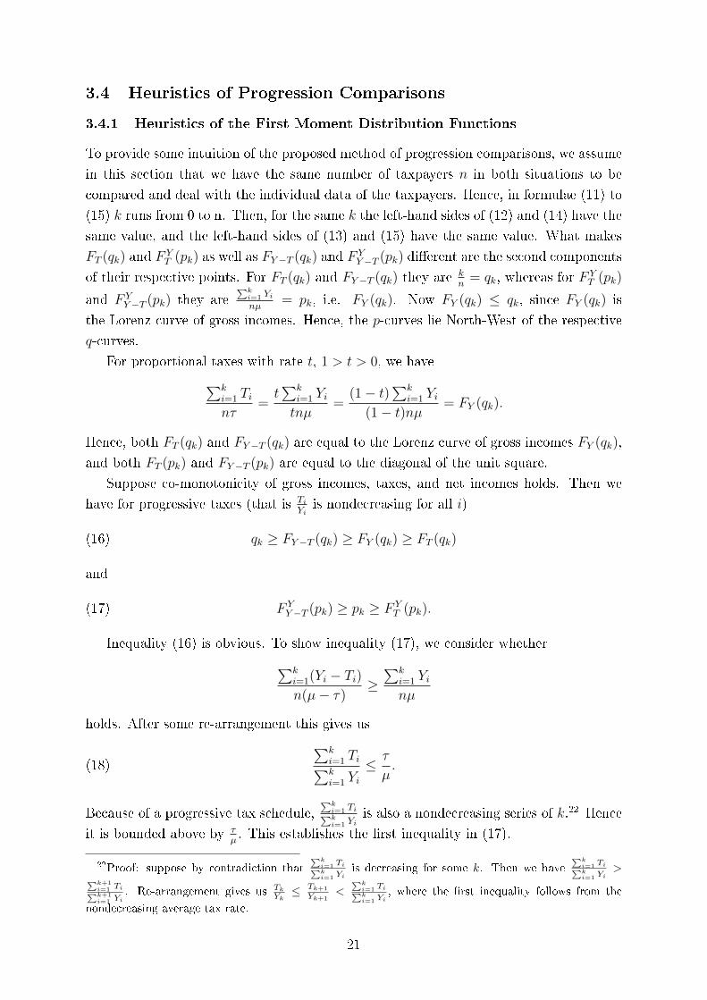
To provide some intuition of the proposed method of progression comparisons, we assume

in this section that we have the same number of taxpayers n in both situations to be

compared and deal with the individual data of the taxpayers. Hence, in formulae (11) to

(15) k runs from 0 to n. Then, for the same k the left-hand sides of (12) and (14) have the

same value, and the left-hand sides of (13) and (15) have the same value. What makes

FT (qk) and FYT (pk) as well as FY−T (qk) and F

YY−T (pk) di�erent are the second components

of their respective points. For FT (qk) and FY−T (qk) they are kn

= qk, whereas for FYT (pk)

and F YY−T (pk) they are

∑ki=1 Yinµ

= pk, i.e. FY (qk). Now FY (qk) ≤ qk, since FY (qk) is

the Lorenz curve of gross incomes. Hence, the p-curves lie North-West of the respective

q-curves.

For proportional taxes with rate t, 1 > t > 0, we have∑ki=1 Tinτ

=t∑k

i=1 Yitnµ

=(1− t)

∑ki=1 Yi

(1− t)nµ= FY (qk).

Hence, both FT (qk) and FY−T (qk) are equal to the Lorenz curve of gross incomes FY (qk),

and both FT (pk) and FY−T (pk) are equal to the diagonal of the unit square.

Suppose co-monotonicity of gross incomes, taxes, and net incomes holds. Then we

have for progressive taxes (that is TiYi

is nondecreasing for all i)

(16) qk ≥ FY−T (qk) ≥ FY (qk) ≥ FT (qk)

and

(17) F YY−T (pk) ≥ pk ≥ F Y

T (pk).

Inequality (16) is obvious. To show inequality (17), we consider whether∑ki=1(Yi − Ti)n(µ− τ)

≥∑k

i=1 Yinµ

holds. After some re-arrangement this gives us

(18)

∑ki=1 Ti∑ki=1 Yi

≤ τ

µ.

Because of a progressive tax schedule,∑ki=1 Ti∑ki=1 Yi

is also a nondecreasing series of k.22 Hence

it is bounded above by τµ. This establishes the �rst inequality in (17).

22Proof: suppose by contradiction that∑k

i=1 Ti∑ki=1 Yi

is decreasing for some k. Then we have∑k

i=1 Ti∑ki=1 Yi

>∑k+1i=1 Ti∑k+1i=1 Yi

. Re-arrangement gives us Tk

Yk≤ Tk+1

Yk+1<

∑ki=1 Ti∑ki=1 Yi

, where the �rst inequality follows from the

nondecreasing average tax rate.

21

The second part of inequality (17) comes from checking whether∑ki=1 Yinµ

≥∑k

i=1 Tinτ

holds. It is immediately seen that this reduces to (18) and, thus, establishes the second

part of inequality (17).

Hence, for co-monotonicity and progressive taxation F YY−T (pk) lies above and F

YT (pk)

below the diagonal of the unit square. For co-monotonicity and increasing, but regressive,

taxation the opposite inequality signs hold in the inequalities (16) and (17).

When re-ranking occurs, co-monotonicity is violated, and the resulting concentration

curves below the diagonal exhibit less curvature, and the concentration curves above

the diagonal [this is F YY−T (pk)] more curvature, i.e., the �rst group moves closer to the

diagonal and the second further away from the diagonal. Although cases such that the

inequalities (16) and (17) are violated may be constructed, they hold in most cases for

empirical data. Recall that Peichl and Schäfer (2008, pp. 9-12) found that the re-ranking

e�ects are not spectacular.

3.4.2 Heuristics of Uniformly Greater Progression

Concerning De�nitions 1 to 6, for empirical data the net incomes are more equally dis-

tributed than the gross incomes, and gross incomes are more equally distributed than

taxes. This means that the q-curves for net incomes exhibit the least curvature, followed

by the q-curves for gross incomes, with the q-curves for taxes having the most curvature.

As to the p-curves, they become the diagonal for gross incomes, a convex curve for taxes,

and a concave curve for net incomes.

Uniformly Greater Tax Progression: Formally Stated De�nition 1 states that

(Y 1, T 1) is more progressive than (Y 2, T 2), if the �rst moment distribution function of T 1

with respect to q lies below that of T 2. The degree of higher progression can be measured

by taking the di�erence between these curves, which in turn can be captured by the area

under the curve FT 2(qk)− FT 1(qk) keeping in mind the sign of the di�erence. De�nition

2 does the same for the �rst moment distribution functions of taxes with respect to p.

Because of our above observation we would expect a smaller di�erence on average for the

p-curves than for the q-curves.

According to De�nition 3, (Y 1, T 1) is more progressive than (Y 2, T 2), if the �rst

moment distribution function with respect to qk of the net incomes (Y 1 − T 1) lies above

that of (Y 2 − T 2). That is, for each quantile qk (except at the end points) the quantile's

fraction of the total net income is higher under (Y 1, T 1) than under (Y 2, T 2). A similar

Now, Tk

Yk<

∑ki=1 Ti∑ki=1 Yi

is equivalent to Tk∑k−1

i=1 Yi < Yk∑k−1

i=1 Ti, and, hence,Tk−1

Yk−1≤ Tk

Yk<

∑k−1i=1 Ti∑k−1i=1 Yi

,

where the �rst inequality follows from the nondecreasing average tax rate. Backward induction shows

for k = 2 that T2

Y2< T1

Y1, which contradicts the condition of nondecreasing average tax rates. Q.E.D.

22

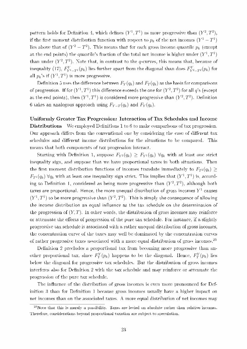
pattern holds for De�nition 4, which de�nes (Y 1, T 1) as more progressive than (Y 2, T 2),

if the �rst moment distribution function with respect to pk of the net incomes (Y 1− T 1)

lies above that of (Y 2 − T 2). This means that for each gross income quantile pk (except

at the end points) the quantile's fraction of the total net income is higher under (Y 1, T 1)

than under (Y 2, T 2). Note that, in contrast to the q-curves, this means that, because of

inequality (17), F YY 1−T 1(pk) lies further apart from the diagonal than does F Y

Y 2−T 2(pk) for

all pk's if (Y 1, T 1) is more progressive.

De�nition 5 uses the di�erence between FY (qk) and FT (qk) as the basis for comparisons

of progression. If for (Y 1, T 1) this di�erence exceeds the one for (Y 2, T 2) for all q's (except

at the end points), then (Y 1, T 1) is considered more progressive than (Y 2, T 2). De�nition

6 takes an analogous approach using FY−T (qk) and FY (qk).

Uniformly Greater Tax Progression: Interaction of Tax Schedules and Income

Distributions We employed De�nitions 1 to 6 to make comparisons of tax progression.

Our approach di�ers from the conventional one by considering the case of di�erent tax

schedules and di�erent income distributions for the situations to be compared. This

means that both components of tax progression interact.

Starting with De�nition 1, suppose FY 2(qk) ≥ FY 1(qk) ∀qk with at least one strict

inequality sign, and suppose that we have proportional taxes in both situations. Then

the �rst moment distribution functions of incomes translate immediately to FT 2(qk) ≥FT 1(qk) ∀qk with at least one inequality sign strict. This implies that (Y 1, T 1) is, accord-

ing to De�nition 1, considered as being more progressive than (Y 2, T 2), although both

taxes are proportional. Hence, the more unequal distribution of gross incomes Y 1 causes

(Y 1, T 1) to be more progressive than (Y 2, T 2). This is simply the consequence of allowing

the income distribution an equal in�uence as the tax schedule on the determination of

the progression of (Y, T ). In other words, the distribution of gross incomes may reinforce

or attenuate the e�ects of progression of the pure tax schedule. For instance, if a slightly

progressive tax schedule is associated with a rather unequal distribution of gross incomes,

the concentration curve of the taxes may well be dominated by the concentration curves

of rather progressive taxes associated with a more equal distribution of gross incomes.23

De�nition 2 precludes a proportional tax from becoming more progressive than an-

other proportional tax, since F YY (pk) happens to be the diagonal. Hence, F Y

T (pk) lies

below the diagonal for progressive tax schedules. But the distribution of gross incomes

interferes also for De�nition 2 with the tax schedule and may reinforce or attenuate the

progression of the pure tax schedule.

The in�uence of the distribution of gross incomes is even more pronounced for Def-

inition 3 than for De�nition 1 because gross incomes usually have a higher impact on

net incomes than on the associated taxes. A more equal distribution of net incomes may

23Note that this is merely a possibility. Taxes are levied on absolute rather than relative incomes.

Therefore, considerations beyond proportional taxation are subject to speculation.

23

result from a progressive tax schedule and/or from a more equal distribution of gross

incomes. Only if the income distribution is the same can we attribute greater progression

to the tax schedule alone. The other end of the gamut is established by the case of a

proportional tax for which greater progression is wholly determined by the distribution

of gross incomes. In e�ect, the in�uence of the distribution of gross incomes is at most

pronounced for the net incomes, which, in turn governs the behavior of De�nition 3.

De�nition 4 precludes a proportional tax from becoming more progressive than an-

other proportional tax, since F YY−T (pk) becomes equal to F Y

Y (pk), which is the diago-

nal. For progressive tax schedules, F YY−T (pk) lies, according to (17), above the diagonal.

Comparisons of tax progression are again heavily in�uenced by the distribution of gross

incomes. This e�ect is even more pronounced for De�nition 4 than for De�nition 2.

Re-arranging De�nitions 5 and 6, we have the terms [FY (qk)−FT (qk)] and [FY−T (qk)−FY (qk)], respectively. Recall that these terms are zero for proportional taxes. Hence,

De�nitions 5 and 6 become zero for proportional tax schedules. In a way, De�nitions 5

and 6 calibrate for the gross income distributions, as they just consider the deviations of

the �rst moment distribution of the gross incomes from the �rst moment distributions

of the taxes or net incomes, respectively. Hence, the in�uence of the distributions of

gross incomes is partly neutralized. Moreover, at �rst sight De�nitions 5 and 6, as they

were formulated above, may invoke the wrong conclusion that they provide a separation

between the in�uence of the income distribution on the one hand, and the tax schedule on

the other. But this impression is not correct, since the terms FT (qk) and FY−T (qk) are by

themselves in�uenced by the respective gross income distributions. This is also evidenced

from Theorems 1 to 3, which show us that the tax schedules and the income distributions

are intrinsically amalgamated so that a straightforward separation of their in�uence is

not at hand.24 Hence, De�nitions 5 and 6 may be considered a second-best approach at

separating the in�uence of the distributions of gross incomes and tax schedules. Here

also the tax terms and the net income terms depend on the income distribution, which

prevents a clear-cut separation between these in�uences.

4 Data and Results

Our empirical investigation addresses several problems:

24For the su�cient conditions, Theorems 2 and 3 may at �rst sight impart the impression of separate

in�uences of the elasticities of the tax schedules or net incomes on the one hand, and the elasticities χ(p)

and Ψ(q) on the other. However, this impression obscures that the elasticities ε(·) and η(·) themselves

depend in intricate ways on the income distributions (which applies also to Theorem 1). [Note that things

are di�erent for the analysis in terms of income. For the su�cient conditions in terms of taxes and net

incomes we observe the sum of the elasticity of the density function of the income distribution on the

one hand, and the tax elasticity or the residual income elasticity on the other; see Seidl (1994, pp. 347-

8). However, this analysis applies only to cases of identical monetary units and identical support of the

income distributions involved.] The work of Dardanoni and Lambert (2002) may also be viewed under

the aspect of separating tax schedules and income distributions. These authors employ deformation

functions to mimic the income distribution of the other country to be compared. However, this possible24

Firstly, recall that the method of comparing tax progression which we proposed de-

termines not a complete, but only a partial ordering. This provokes the question whether

it is of major relevance because it might be that the tax schedules associated with their

respective income distributions are so involved that only few clear-cut dominance rela-

tions emerge. In other words: is our method of comparison of tax progression in the real

world only a will-o'-the-wisp, or can it command major occurrence?

Secondly, if our �rst question is responded in the a�rmative, what is the relative

performance of the six proposed measures of the comparison of tax progression? Are

there interrelationships? What are the economic message and content of these methods?

Thirdly, what is the relative importance of su�cient and necessary conditions of com-

parisons of tax progression? For which fraction of greater tax progression the relative

concentration curves would be strictly convex or concave, and for which they would just

not cross the diagonal of the unit square without being strictly convex or concave? If

the respective elasticity conditions do not hold, can we safely assume that greater tax

progression is unlikely or can we expect it to be rather common?

Fourthly, what is the pattern of comparisons of tax progression when dominance

relations do not hold? Do we mainly encounter bifurcate or more intricate progression

patterns? Is there a change of the progression pattern at a unique threshold, or do we

have a whole series of changes of the progression relations?

Our analyses are carried out for both household data and equivalized data. We used

the respective data from the Luxembourg Income Study database (see LIS (2010)). We

mainly focus on international comparisons of tax progression, but also carry out intertem-

poral comparisons of tax progression for selected countries. Furthermore, we perform a

sensitivity analysis with respect to the LIS equivalence scale parameter. To address these

and related questions, we need household data for both gross and net incomes. In addi-

tion to that, for intertemporal comparisons for each country we required the data from

at least three recent survey periods (�waves� in LIS terminology; in particular, we used

waves III up to VI if the respective data allowed). Data sets showing gross incomes, direct

taxes, payroll taxes, and net incomes were available just for 15 countries out of which we

took 13, representing in our view the most salient ones. As a shorthand terminology we

will use �taxes� to refer either to direct taxes or to direct taxes plus payroll taxes.

We will start with a short description of handling the LIS data, then will report six

tables with pairwise progression comparisons for De�nitions 1 to 6, followed by comments

on six tables with summary results. Then we will analyze sixteen selected graphs for

progression comparison related to comparing Germany, the United Kingdom, and the

United States, as well as comparing Germany and Sweden, in terms of household incomes

with direct taxes and direct taxes plus payroll taxes, and in terms of equivalized data for

direct taxes and direct taxes plus payroll taxes. To provide an overview of our �ndings

way of decomposition works only for isoelastic deformation functions to secure independence of the

baseline distribution (see also Footnotes 1 and 14).

25

for international progression comparisons, we will present Hasse diagrams. Finally, we

provide examples of intertemporal progression comparisons and sensitivity results with

respect to the parameter of the Luxembourg equivalence scale.

Note that this paper is entirely devoted to numerical analyses. We defer the statisti-

cal analysis to subsequent work due to much higher computation requirements for data

processing on the LIS side (see also Footnote 30).

4.1 Handling LIS Data

Our empirical analysis resorts to micro data drawn from the LIS (2010) database. It is

a cross-national data archive located in Luxembourg.25 Currently it includes micro data

from more than 30 countries, most of which are OECD member states. The data sets

are organized into �waves� of about �ve years each, starting with Wave I in 1980 and the

most recent being Wave VI (around 2004). The micro data from the di�erent surveys

is harmonized and standardized in order to facilitate comparative research. For many

countries, however, only a limited number of waves is available, and even if a data set is

available, not all income variables are included. In particular, gross incomes, direct taxes

and payroll taxes are available only for 15 countries, of which we used 13 in our study.

Table 1 gives a summary of the countries and waves used. The countries are listed

according to the country codes which were used to access the data sets. Columns III to

VI list the years to which the data sets, included in the respective waves, refer to. For

international comparisons, we took Wave V (around 2000) because of its relative recency

and as maximizing the number of available country data. We also included France, but

due to data availability, we had to rely on wave 1994. Poland's Wave III data set was

not included as we deem it being too close to the fall of the Iron Curtain.

Within the data sets, at the household level LIS reports, inter alia, gross income

(GI), disposable net income (DPI), income taxes (V11) and mandatory payroll taxes

(PAYROLL). In what follows, we employ two di�erent net income de�nitions. Net income

is de�ned either in accordance with LIS as DPI=GI−(V11+PAYROLL), or it is rede�ned

by us as GI−V11, i.e., the analysis is based on taxes only.26 It should be noted, however,

that V11 in some cases already includes social security contributions if these were lumped

together in the original data set before adding it to LIS. Furthermore, some countries like

25For more information about the LIS database see Smeeding et al. (1985), Smeeding (2004), and

Atkinson (2004). For illustrative examples of applications of the LIS database see, e.g., Allegrezza et al.

(2004), Bardasi (2004), Bronchetti and Sullivan (2003), Gornick (2004), Förster and Vleminckx (2004),

and Mahler and Jesuit (2006).26This means that taxes include so-called clawbacks. i.e., taxes which return to government part of

the transfer. Prasad and Deng (2009, p. 439) remark: �This means that where transfers are high, taxes

on transfers may be high, but this is not `true' tax, simply a reduction in the amount of transfer given.

To achieve a measure of true tax paid, then, the amount of clawbacks should be subtracted from the

total tax paid.� However, we opine that clawbacks are an integral part of the tax system. In contrast to

Prasad and Deng (2009) we also do not consider indirect taxes in our investigations.

26

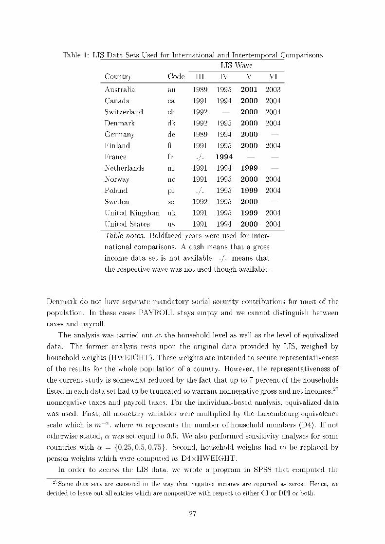
Table 1: LIS Data Sets Used for International and Intertemporal Comparisons

LIS Wave

Country Code III IV V VI

Australia au 1989 1995 2001 2003

Canada ca 1991 1994 2000 2004

Switzerland ch 1992 � 2000 2004

Denmark dk 1992 1995 2000 2004

Germany de 1989 1994 2000 �

Finland � 1991 1995 2000 2004

France fr ./. 1994 � �

Netherlands nl 1991 1994 1999 �

Norway no 1991 1995 2000 2004

Poland pl ./. 1995 1999 2004

Sweden se 1992 1995 2000 �

United Kingdom uk 1991 1995 1999 2004

United States us 1991 1994 2000 2004

Table notes. Boldfaced years were used for inter-

national comparisons. A dash means that a gross

income data set is not available. ./. means that

the respective wave was not used though available.

Denmark do not have separate mandatory social security contributions for most of the

population. In these cases PAYROLL stays empty and we cannot distinguish between

taxes and payroll.

The analysis was carried out at the household level as well as the level of equivalized

data. The former analysis rests upon the original data provided by LIS, weighed by

household weights (HWEIGHT). These weights are intended to secure representativeness

of the results for the whole population of a country. However, the representativeness of

the current study is somewhat reduced by the fact that up to 7 percent of the households

listed in each data set had to be truncated to warrant nonnegative gross and net incomes,27

nonnegative taxes and payroll taxes. For the individual-based analysis, equivalized data

was used. First, all monetary variables were multiplied by the Luxembourg equivalence

scale which is m−α, where m represents the number of household members (D4). If not

otherwise stated, α was set equal to 0.5. We also performed sensitivity analyses for some

countries with α = {0.25, 0.5, 0.75}. Second, household weights had to be replaced by

person weights which were computed as D4×HWEIGHT.

In order to access the LIS data, we wrote a program in SPSS that computed the

27Some data sets are censored in the way that negative incomes are reported as zeros. Hence, we

decided to leave out all entries which are nonpositive with respect to either GI or DPI or both.

27

values of FY (q), FT (q), and so on, at 20 equally spaced quantiles of the unit interval

and printed back these results for every data set (country and year), for taxes and taxes

plus payroll taxes for both household and equivalized data. We had to use this approach

because direct access to LIS data is not permitted. We then wrote a Visual Basic macro

to facilitate processing of the LIS output o�ine.

4.2 Heuristics of Progression Comparisons for Grouped Data

Our formulae and de�nitions presented in Section 3.3 and discussed in Section 3.4 were

cast in terms of individual data. Although this approach appears prima facie as the proper

one, we could not apply it to our empirical work because, �rst, LIS does not allow direct

access to its data (hence we had to compute all the aggregates for our analysis online,

which presents a challenge since a resource-demanding program code is not welcomed

by LIS), and, second, the numbers of taxpayers in the populations to be compared are

typically di�erent. This last feature would have necessitated tedious ad hoc interpolation

procedures for all pairwise comparisons. To deal with both issues in a more expedient

way, we employed the following approach using grouped data.

We divided the unit interval into 20 shares, i.e., taking �ve-percent steps28 as equally

spaced quantiles for q in terms of population shares and for p in terms of income shares.

This assumption implies that the respective transformed indices j coincide for all respec-

tive situations to be compared in formulae (11) to (15), that is j = 0, 1, . . . , 20. For our

work with LIS data this approach has the decisive advantage that we are able to quickly

process the data for all 13 countries at the LIS server (the critical time consuming part

of our computations) and then analyze the results o�ine.

We started our procedure by arranging the raw data (taxes and associated net in-

comes) in our sample in the increasing order of the associated gross incomes; for equiv-

alized incomes the data were re-arranged in the increasing order of equivalized gross

incomes. Next, we divided the unit intervals, which correspond to the ranges of the

cumulative distribution function for gross incomes, into 20 equally spaced �ve-percent

groups for the analysis in terms of population quantiles q, and in terms of income quan-

tiles p, respectively. Then we took the respective shares of aggregate taxes, gross and

net incomes associated with these �ve-percent quantiles. Thus we obtained the values

for qj, pj, FY (qj), FT (qj), FY−T (qj), FYT (pj), and F

YY−T (pj) for our grouped data, where

j = 0, 1, . . . , 20.

But the curves for grouped data deviate from the curves for individual data in sev-

eral respects. For individual data, as we observed in Section 3.4.1, if we have the same

28As compared to other empirical work, this is a rather �ne grid. Sala-i-Martin (2006, pp. 355 and

357), for instance, had to work with quintiles and had to resort to widespread data interpolations for

carrying out his ambitious study. Bishop et al. (1991a, p. 464) worked with deciles for their construction

of Lorenz curves, arguing that �increasing the number of quantiles does not necessarily improve the

quality of the overall test� (p. 476, Footnote 5).

28

number of income recipients and (for the same value of k) the same partial sums for

both the q-curve and the p-curve, then we have the same corresponding values on either

curve's ordinate; hence, by pk ≤ qk, the curves di�er only by their corresponding values

on the abscissa. For grouped data, we apparently have the same equally distanced quan-

tiles on the abscissa; therefore, the q-curve and the p-curve di�er with respect to their

corresponding values on the ordinate.

Consider now the q and p curves for taxes for grouped data. For the lower income

strata, the �ve-percent quantiles contain more taxpayers in terms of p than in terms of

q. In turn, this implies also more relative tax revenue for the p-curve as compared with

the q-curve. Hence, for the lower income strata we have F YT (pj) ≥ FT (qj) for pj = qj.

This means that the tax revenue associated with upper quantiles is smaller in terms of p

than in terms of q. Hence, the p-curve for the taxes has a steeper slope than the q-curve

for the lower quantiles and a �atter slope for the upper quantiles. But the q-curve can

never cut the p-curve from below in the interior of the unit square. This is easily seen:

obviously we have for the gross incomes FY (q) ≤ p = F YY (p) for q = p. Hence, for q = p

the gross income shares according to q can never exceed the gross income share according

to p. For a progressive tax schedule this implies that FT (q) ≤ F YT (p) for q = p. Moreover,

note that neither curve crosses the diagonal.

Consider the q and p curves of net incomes for grouped data. For the q-curves,

basically the same reasoning applies as to Lorenz curves29 because the net income shares

increase for increasing quantiles. Hence, FY−T (qj) lies below the diagonal. For the p-

curves, basically the same reasoning applies as for the analysis of inequality (18). For the

individual data we can de�ne an increasing series k1, k2, . . . , k20, such that∑kji=1 Yinµ

−∑kj−1

i=1 Yinµ

' 0.05, j = 1, . . . , 20,

due to the �neness of the LIS data. Replace now kj by j and[∑kji=1(Yi − Ti)n(µ− τ)

−∑kj−1

i=1 (Yi − Ti)n(µ− τ)

]by F Y

Y−T (pj),

then (17) translates into our grouped data and, hence, inequality (18) translates into our

grouped data as well.

This means that our analyses are carried out for De�nitions 1 to 6 in terms of grouped

data for qj and pj, where j = 0, 1, . . . , 20.

Separation of tax progression with respect to the in�uence of the income distribution

on the one hand and the tax schedule on the other was discussed in section 3.4.2. As

concerns empirical data, we have to add another problem. Even for the case of identical

monetary units, identical support of the income distribution, and con�nement to the

29See Gastwirth and Glauberman (1976) for errors in estimating Lorenz curves when grouped date are

used instead of individual data.

29

su�cient conditions, we would need the exact tax schedule to disentangle the in�uence

of the income distribution and the tax schedule. However, the nominal tax schedule

would not su�ce for this purpose. We would have to capture also the administration

of a going tax schedule. All tax codes contain many tax bene�ts, itemized deductions

from the tax base, etc. While these instances are captured by the real micro data of

taxation, they are not captured by the nominal tax schedule. Yet they constitute a

major element of real tax progression. This was also one of our reasons to use the LIS

data instead of simulated data, such as, e.g., the EUROMOD data. Hence, even under

favorable theoretical conditions, decomposition of tax progression into a term dealing

with the income distribution and a term dealing with taxation is limited by empirical

data problems.

4.3 Numerical Progression Comparisons

Categorical data of progression relationships just inform on progression dominance, bi-

furcate progression dominance, or multiple crossings of the respective curves. Curve

di�erences inform also on the intensities of progression dominance. We present �rst our

categorical results and thereafter progression intensities for selected countries.

The categorical results of our international comparisons of tax progression are pre-

sented in Tables 2 to 7. For these tables we use the following notation:

D and d denote progression dominance: D means that the country in the row dominates

the country in the column with respect to progression; d means that the country in the

row is dominated by the country in the column with respect to progression. Note that the

entries D and d are asymmetric: a D in cell (i, j) implies a d in cell (j, i), and vice versa.

A superscript C indicates convexity or concavity of the associated relative concentration

curve, i.e, that the respective su�cient conditions (elasticities) of Theorems 1 to 3 hold.

R and r denote bifurcate progression: R means that the country in the row is more

progressive than the country in the column for the lower income strata and less progressive

for the upper income strata; r means that the country in the row is less progressive than

the country in the column for the lower income strata and more progressive in the upper

income strata. Note again that the entries R and r are asymmetric.

# denotes multiple changes of the progression pattern.

4.3.1 International Progression Comparisons: Categorical Summary Results

Tables 2 to 7 present the results corresponding to De�nitions 1 to 6. Each cell in these

tables contains four entries: the entries in the �rst line refer to household data, the entries

in the second line to equivalized data using the Luxembourg equivalence scales m−α with

α = 0.5. The left-hand side entries in a cell refer to direct taxes only, while the right-hand

30

side entries to direct taxes plus payroll taxes (which consist mainly of employees' share

in social security contributions).

Inspection of the cells of Tables 2 to 7 shows that only few left-hand side and right-

hand side columns di�er within each cell. Disregarding the C-superscripts, which just

indicate that the respective curve di�erences have a unique extremum, still increases the

similarity of the columns within each cell. This means that comparative progression is

not changed much if we extend the direct taxes by payroll taxes. This is remarkable

since payroll taxes are by and large proportional to the incomes for the lower and middle

income strata. For incomes exceeding some benchmark payroll taxes on incomes beyond

this benchmark expire altogether. Moreover, for the lower income strata they are usu-

ally considerably higher than the direct taxes. This implies that they have a regressive

e�ect on overall tax progression (for the e�ect of payroll taxes in isolation see Peichl and

Schäfer (2008, pp. 13-4)). On top of that, their structure may be di�erent for di�erent

countries. An exceptional case is Denmark, where social security contributions are neg-

ligible, because most social expenditures are paid out of the tax revenue. Nevertheless,

our results show few di�erences in comparative progression for direct taxes and direct

taxes plus payroll taxes.

Basically the same observation applies to the rows within each cell. Although being

less similar than the columns, most of them have similar appearance. This means that

replacing taxes and net incomes for household data by equivalent taxes and equivalent

net incomes does not cause dramatic changes in the comparative progression pattern,

although the changes are more pronounced than comparisons between direct taxes only

and direct taxes plus payroll taxes. Note that equivalized incomes and taxes tend to be

more equally distributed than household incomes and taxes (cf. Peichl et al., 2009a,b).

Countries with a higher proportion of large households are more likely to experience

changes between the �rst and the second rows in the cells of the tables.

Tables 8 to 11 survey the results of the comparisons across De�nitions 1 to 6. They

show us that for international comparisons of uniform tax progression, progression domi-

nance is the rule rather than the exception. In about to two thirds of all 312 international

comparisons, uniform progression dominance holds.30 Among these cases, for between

30Note that these are the results of our numerical calculations. As our curves do not draw on the data

universe, but on samples only, the question arises whether curve crossings are statistically signi�cant.

Whereas Atkinson (1970, p. 258) had asserted that for comparisons among twelve countries �in only

16 out of 66 cases do the Lorenz curves not intersect�, Bishop et al. (1991a, p. 462) found statistically

signi�cant intersections of Lorenz curves only in three percent of all cases, whereas 97 percent of the

Lorenz curves were ranked; in contrast to that, simple numerical comparisons would have ranked only

some 75 percent of the comparisons of Lorenz curves. This result holds under the assumption that

the di�erences between the population Lorenz ordinate and the sample Lorenz ordinate are normally

distributed (see also Bishop et al. (1991b), who showed impressive results also for the double criterion of

Lorenz dominance and higher mean income). This means for our results that we might end up with even

more dominance relations if we required curve intersections to be statistically signi�cant. On the other

hand, Dardanoni and Forcina (1999) showed using Monte-Carlo simulations that the statistical power

31

60.78 and 83.05 percent of progression dominance the respective curve di�erences have a

single extremum, which means that the su�cient conditions of convexity or concavity of

the associated relative concentration curves hold. However, in between 16.95 and 39.22

percent of cases do we observe that the su�cient conditions of Theorems 1 to 3 do not

hold, although the associated relative concentration curves do not cross the diagonal in

the unit square.

Uniform progression dominance does not hold for about one third (exactly 32.69

percent) of all cases only. Among these cases we observe between 65.38 and 84.21 percent

for which bifurcate progression holds. This means that in these situations there is a unique

benchmark such that uniform progression dominance for one country holds up to this

benchmark and reverses for the quantiles exceeding this benchmark for the other country.

With respect to all cases this means that only for between 3.85 and 11.54 percent do we not

have clear-cut patterns of progression dominance: the associated relative concentration

curves have in these cases multiple crossings with the diagonal of the unit square or,

alternatively, the respective curve di�erences change their sign more than once. This

is negligible as compared with the two thirds of all cases in which uniform progression

dominance holds and with more than one �fth of all cases in which bifurcate progression

holds.

Progression dominance is a transitive relation. Hence, we can arrange the strict

progression dominance relationship of Tables 2 to 7 in terms of Hasse diagrams, which are

presented in Figures 3 to 26. We have Hasse diagrams for each of our six de�nitions and

each of our four data sets, which produces 24 �gures. At the top of these �gures we �nd the

countries with the highest progression dominance, at the bottom those countries which

are progression dominated by most other countries, but do not progression dominate

other countries. Except for Figures 5, 11, 17, and 23, we �nd Switzerland and Poland

at the bottom, and Denmark, Sweden, Norway, Finland, and the United Kingdom in the

lower parts of the �gures. At the top we �nd Germany, the United States, Australia,

Canada, and the Netherlands. Only Figures 5, 11, 17, and 23 put everything upside

down. All these �gures concern De�nition 3, which turns out as an outlier among our six

de�nitions. This phenomenon will subsequently crop up also in our other �ndings.

4.3.2 International Progression Comparisons: Consistency among Progres-

sion Concepts

Tables 12 and 13 report the robustness of progression comparisons across our six de�ni-

tions. These tables show us that full consistency is rather rare: it varies between 2.56

and 8.97 percent for progression dominance31 and between 5.13 and 15.38 percent for

of the Lorenz curve as a test device is low. However, in the present paper our focus is on the numerical

analysis. The respective statistical tests will be conducted in our future research.31A 100 percent full consistency for a set of de�nitions would mean that any one de�nition out of

this set can represent the rest, while the rest would become super�uous because all measure the same

32

bifurcate progression. Note that full consistency is highest for taxes plus payroll taxes for

equivalized data. However, when we look for at least four consistencies, the consistency

rates increase to numbers between 34.64 and 48.71 percent for progression dominance

and to numbers between 62.22 and 70.52 percent for bifurcate progression.

Table 14 contains rough indications of similarities and dissimilarities among the pro-

gression comparison concepts.32 This table is based on pairwise comparisons of the entries

in Tables 2 to 7 counting the dominance and bifurcate relationships which are identical

between pairs of tables. The �rst entries in the cells of Table 14 contain the percentages

(as averages of all four datasets) of congruence of the respective D's and R's in the cells of

the pairs of the compared tables, the second entries contain the percentages (as averages

of all four datasets) of cases in which a D or R is not matched by the respective symbol in

the other table.33 Multiple crossings were ignored. We observe strong similarity of 83.66

percent between De�nitions 1 and 2, although De�nition 1 is expressed in terms of q and

De�nition 2 in terms of p; note that both concern de�nitions in terms of taxes. Strong

similarities are also observed between De�nitions 1 and 4 (63.46 percent), De�nitions 1

and 5 (65.06 percent), De�nitions 2 and 4 (60.90 percent), De�nitions 2 and 5 (67.62

percent), De�nitions 4 and 6 (69.23 percent), and De�nitions 5 and 6 (58.97 percent).

The similarities between De�nitions 1 and 2 on the one hand, and De�nitions 5 on the

other, can be explained by their common casting in terms of taxes. The similarities be-

tween De�nitions 4 and 6 can be explained because they are cast in terms of net incomes.

However, the similarities between De�nitions 1 and 2 on the one hand, and De�nition 4

on the other would not have been expected a priori because De�nitions 1 and 2 are cast

in terms of taxes and De�nition 4 is cast in terms of net incomes. Moreover, De�nition

1 is based on q, whereas De�nitions 4 is based on p. Hence, Table 14 suggests that we

have two (overlapping) similarity clusters: De�nitions 1, 2, 4, and 5 on the one hand, and

De�nitions 4, 5, and 6 on the other. This is also con�rmed upon checking higher-order

consistencies (not reported in the present text).

Table 14 demonstrates also the particularity of De�nition 3, which has very high

rates of dissimilarity with the other de�nitions. It behaves as a complete outlier, which

indicates that it measures phenomena which are dissimilar as compared with the other

de�nitions. Interestingly enough, even De�nition 4, which is, on theoretical grounds, the

one most related to De�nition 3, exhibits lower dissimilarity rates with respect to all

other de�nitions than does De�nition 3.

Let us for a moment set aside De�nition 3 and concentrate on the other de�nitions.

When looking at Tables 2-3 and 6-7 as well as at Figures 3-26 (except Figures 5, 11,

phenomenon. Hence, less than full consistency justi�es a multiple of measures for progression comparisons

because all measure di�erent traits.32Note that consistency between our de�nitions depends on the data used. Hence, the present analysis

re�ects the data used for this study.33Note that we consider a pair of de�nitions similar if it is either D or R [d or r], but not the opposite

(], d, r) [],D,R], respectively.

33

17, and 23), it is striking to see that �high tax� (as conventionally perceived) countries

like Sweden and Denmark, medium tax countries like the United Kingdom, and low

tax countries like Switzerland and Poland are all classi�ed as less progressive than most

other countries. Furthermore, high tax countries like Germany, medium tax countries like

France, and low tax countries like the United States are classi�ed as more progressive

than most other countries. This is because the measures in this paper are developed

for comparing uniform tax progression, not the level of taxation. Sweden and Denmark

have taxes that reach a high percentage of income rather fast and remain there, which is

more akin to proportional taxation; the same pattern applies to the United Kingdom for

a medium tax burden, and to Switzerland and Poland for a low tax burden. In contrast

to that, the income interval for which taxation is steadily increasing as a percentage of

income is comparatively extensive in Germany, in France, and in the United States. This

explains their dominance with respect to comparisons of tax progression. For similar

results using another approach see Peichl and Schäfer (2008, pp. 8-12).

Let us now focus on the discrepancy between De�nition 3 and the other de�nitions.

To illustrate, we single out the case of De�nitions 3 and 4 which have a high inconsistency

rate of 71.47 percent according to Table 14, although both de�nitions should be closely

related on theoretical grounds.

First of all we check whether both de�nitions can command plausibility. They can: if

FY 1−T 1(qk) > FY 2−T 2(qk) for all qk, 0 < qk < 1, then the qk × 100 percent of the lowest

income recipients have relatively higher aggregate net income under (Y 1, T 1) than under

(Y 1, T 2); if F YY 1−T 1(pk) > F Y

Y 2−T 2(pk) for all pk, 0 < pk < 1, then the pk × 100 percent of

the recipients of the lowest aggregate gross income have relatively higher aggregate net

income under (Y 1, T 1) than under (Y 1, T 2). Hence, both de�nitions stand a plausibility

test.

Consider now the cells US/CH in Tables 4 and 5. They show for all four entries

that Switzerland has higher uniform progression than the United States according to

De�nition 3, whereas the United States has higher uniform progression than Switzerland

according to De�nition 4. Let us start with the �ctitious assumption that, for whatever

reasons, Switzerland had an equal distribution of gross incomes and a proportional tax,

whereas gross and net incomes were unequally distributed in the United States. Then

we know from Section 3.4.1 that both FY CH−TCH (qk) and FYY CH−TCH (pk) are equal to the

diagonal of the unit square, the �rst by the assumptions of an equal distribution of gross

incomes and a proportional tax, and the second by the assumption of a proportional tax.

However, this case implies higher uniform progression of the income-distribution-cum-

tax system in Switzerland than in the United States according to De�nition 3 and higher

uniform progression in the United States than in Switzerland according to De�nition 4.

Hence, in this case De�nition 4 is accurate, while De�nition 3 is misleading. For moderate

tax progression in one country (in this case: Switzerland) and higher tax progression in

another country (in this case: the United States), this misleading statement of De�nition

34

3 seems to translate to cases for which the distribution of gross incomes in one country

(Switzerland) is su�ciently more equally distributed than in another country (United

States).

Suppose now that the population principle applies and that the same distribution of

gross incomes holds in both countries.34 Then

(19) FY−T 1(qk) ≥ FY−T 2(qk)⇔ F YY−T 1(pk) ≥ F Y

Y−T 2(pk),

if T 1(·) is more progressive than T 2(·). Note that expression (19) follows immediately

from Section 3.4.1.35 Hence, De�nitions 3 and 4 are equivalent for identical gross income

distributions and greater progression depends only on the tax schedules involved.

Let us now consider another extreme case, viz. total progression. A totally progressive

tax schedule consists of just two marginal tax rates, +100% and −100%.36 All incomes

above mean income are taxed away and all incomes below mean income are replenished

by transfers up to mean income. Hence, the net income distribution is equal. Suppose,

Switzerland had a totally progressive tax schedule, while the United States had some

more common progressive tax schedule. Then De�nition 3 correctly indicates higher

progression for Switzerland than for the United States. So does De�nition 4, since τCH =

0 for total progression and by assumption τUS > 0:

kµCH

nµCH=k

n≥∑k

i=1(YUSi − TUSi )

n(µUS − τUS); Y US

i ≥ TUSi .

Therefore, it seems that the ostensibly deviant behavior of De�nition 3 results from

its high sensitivity to the in�uence of the distribution of gross incomes, which may easily

overcompensate the in�uence of the tax schedule and lead to implausible results. In

contrast to De�nition 3, De�nition 4 is less susceptible to the preponderance of the

distribution of gross incomes vis-á-vis the tax schedule. Hence, De�nition 3 has to be

taken with some caution. It is too sensitive with respect to more equal distributions of

net incomes irrespective of how they came about.

4.3.3 International Progression Comparisons: Progression Intensities for Se-

lected Countries

Tables 2 to 7 contain categorical data only; they just report whether we have uniform

progression dominance, bifurcate progression or multiple crossings of the associated rela-

34Switzerland's population is about two percent of the population of the United States. An equal

income distribution in both countries in discrete terms requires therefore 50 income clones in the United

States for each Swiss income recipient. Take an income distribution consisting of one representative out

of the 50 US clones, then both income distributions are identical under the population principle.35The second part of expression (19) may not seem immediate. Consider FY

Y−T 1(pk) ≥ FYY−T 2(pk).

Then there corresponds a unique qk to each pk (recall that qk ≥ pk). Since the same set of taxpayers

has higher relative aggregate net income under pk for T 1, it must also have higher relative aggregate net

income under qk for T 1, as the distribution of gross incomes is the same.36Note that for several reasons we exclude negative taxes for most of our analysis. We use this example

35

tive concentration curves. They are silent about the intensity of progression comparisons.

Information about this aspect is provided by the 312 graphs of international progression

comparisons, where each graph corresponds to one out of the four entries in each cell

of Tables 2 to 7 and contains six curves corresponding to the six concepts of compari-

son of progression as embodied in these six tables. From this set we single out sixteen

for presentation in this paper, of which four cover the comparisons between the United

Kingdom and the United States, four the comparisons between Germany and the United

Kingdom, four the comparisons between Germany and the United States, and four the

comparison between Germany and Sweden.

United Kingdom versus United States Figure 27 depicts the progression compar-

isons for UK 1999 versus US 2000 for the direct taxes and household data. In accordance

with Tables 2 to 7 we see that the US progression dominates the UK for all de�nitions

except De�nition 3. For De�nition 3 tax progression is at �rst higher in the UK than

in the US and switches at q = 0.55 to higher progression for the US than for the UK.

Moreover, note that the curves for De�nitions 3, 4, and 6 show much weaker intensity

than progression dominance according to the other de�nitions.

Figure 28 depicts the progression comparisons for UK 1999 versus US 2000 for the

direct taxes plus payroll taxes and household data. The pattern is the same as for Figure

27 except that the inclusion of payroll taxes now makes the intensity of progression

somewhat less pronounced, as the entries on the ordinate show. Figure 29 depicts the

progression comparisons for UK 1999 versus US 2000 for the equivalized direct taxes and

equivalized incomes. In accordance with Tables 2 to 7 we see that the US progression

dominates the UK for all de�nitions except De�nition 3. For De�nition 3 tax progression

is uniformly higher in the UK than in the US. Figure 30 repeats this pattern for equivalized

direct taxes plus payroll taxes and equivalized incomes.

Germany versus United Kingdom Figure 31 depicts the progression comparisons

for Germany 2000 versus UK 1999 for direct taxes and household data. In accordance

with Tables 2 to 7 we see that German progression dominates the progression in the

United Kingdom for all de�nitions.

Figure 32 depicts the progression comparisons for Germany 2000 versus UK 1999 for

the direct taxes plus payroll taxes and household data. Uniformly greater progression

for Germany vis-á-vis the UK is again observed for all de�nitions except De�nition 1.

For De�nition 1, Germany is more progressive except for the highest 15 percentiles, for

which progression switches to the UK. Note that the ordering of progression dominance

changes when going from direct taxes to direct and payroll taxes: progression dominance

according to De�nition 3 is moderate for direct taxes, but becomes far more pronounced

for direct and payroll taxes, possibly because payroll taxes render the German distribution

here to compare equally distributed net incomes resulting from unequally distributed gross incomes.

36

of net incomes more unequal. Progression dominance according to De�nitions 1, 2, and

5 becomes less pronounced for direct and payroll taxes (De�nition 1 even acts partly in

the direction of less progression for Germany). Figures 33 and 34 repeat this pattern also

for the equivalized data.

Germany versus United States Figure 35 shows higher progression of the German

income-distribution-cum-tax system for De�nitions 2, 3, and 5 (except the 95th percentile)

for direct taxes. De�nitions 4 and 6 do not bear a pronounced message. De�nition 1

indicates higher progression for Germany up to q ∈ (0.6, 0.65) and higher progression for

the United States for the upper income strata.

With respect to direct and payroll taxes, Figure 36 shows higher progression for

Germany only for De�nition 3, whereas De�nitions 1 and 2 indicate higher progression

for the United States. De�nition 5 indicates higher progression for Germany up to q ∈(0.55, 0.6) and higher progression for the United States for the upper income strata. These

shifts re�ect the in�uence of the higher importance of payroll taxes in Germany. Again

De�nitions 4 and 6 do not bear a pronounced message.

The equivalized data in Figures 37 and 38 completely repeat the pattern of Figures

35 and 36, respectively.

Germany versus Sweden It is interesting to compare Germany and Sweden, as Swe-

den is notorious for her high tax burden. Figure 39 shows progression comparison for

direct taxes and household data. We see that Germany is uniformly more progressive

for De�nitions 1, 2, and 5. The other de�nitions are of no major importance; they also

indicate slightly more progression for Germany. This pattern is repeated for direct taxes

and payroll taxes in Figure 40, but now with only about half the intensity as for Figure

39 (compare the entries on the ordinates).

This pattern is repeated also for the equivalized data in Figures 41 and 42, except that

Sweden appears now slightly more progressive according to De�nition 3, which might be

a re�ection of larger family sizes in Sweden.

Hence, the general picture exhibits greater progression in Germany as compared to

Sweden, although Sweden's relative tax burden is higher than Germany's.37

4.3.4 Intertemporal Progression Comparisons

We have data for intertemporal progression comparisons for all selected countries except

France. However, because of space limitations we restrict ourselves here to just three

37Eurostat, Tables tec00018 and tec00019, tell us the percentages of taxes from income and wealth and

social security contributions (in square brackets; employees' and employers' contributions taken together)

of GDP for 2008 (selected �gures): EU 27 mean 13.1 [13.7]; EU 15 mean 13.5 [13.9]; Belgium 16.6 [16.1];

United Kingdom 16.7 [8.4]; Sweden 17.4 [12.00]; Finland 17.5 [12.2]; Iceland 18.3 [2.8]; Norway 22.0 [8.9];

Denmark 29.8 [1.8]. The �gures for Germany are 11.3 [16.4]. This shows that Germany is a low-tax

country with respect to income and wealth taxes and a high-tax country with respect to social security

37

countries, viz. the United States, the United Kingdom, and Germany. Of course, we

could cover only periods for which full sets of comparable data are available. The con�nes

of data availability precludes too long time intervals.38 Interestingly enough, the curve

di�erences for intertemporal progression comparisons have much lower intensity than

the curve di�erences for international progression comparisons. They are in the order

of between one �fth and one tenth of the curve di�erences for international progression

comparisons. This fact is somewhat obscured by curve calibration, but may readily be

seen from the ordinates of the respective �gures.

United States For the United States we have data of waves 1991, 1994, 2000, and

2004. Wave 1991 was in the mid-term of the Bush Senior Administration (1989-93). In his

election campaign, Bush Senior had promised: �Read my lips: no new taxes.� However,

he broke his election pledge, it seems for �nancing the �rst Iraq War, and was not re-

elected. Waves 1994 and 2000 concern the Clinton Administration (1993-2001). Clinton

took over o�ce on January 20, 1993, which ended on January 20, 2001. Clinton was very

successful in reducing budget de�cits, promoting NAFTA, and getting on good terms with

China and Russia. On August 5, 1997, Clinton signed the Tax Relief Act, which meant

a signi�cant tax cut e�ective as of January 1, 1998. Moreover, his administration was

a peaceful period. The very end of his administration was overshadowed by the dotcom

crisis. Wave 2004 concerns the fourth year of the Bush Junior administration. Bush

Junior and Cheney were supposed of favoring the upper income strata of the American

society. Moreover, this period was overshadowed by the second Iraq War, which was

largely �nanced by high budget de�cits. Hence, the progression changes 1991/94 (Bush

Senior to Clinton), 1994/2000 (beginning and end of the Clinton Administration), and

2000/04 (Clinton to Bush Junior) are of interest.

Table 15 provides a concise summary on the categorical data of comparisons of tax

progression. We use the following notation: Bsen means �Bush Senior�, C* means �Clin-

ton 1994�, C** means �Clinton 2000�, and Bjun means �Bush Junior�. An arrow means

that the �rst entry is taken as a starting point and the second entry as the end point

of the comparison. For instance, the entry d [D] under 91→94 and Bsen → C*, respec-

tively, means that the tax system in 1991 under the Bush Senior Administration was

less progressive [more progressive] than in 1994 under the Clinton Administration. The

�rst three double columns in Table 15 concern the comparisons over adjoining periods,

the second three double columns concern comparisons over longer periods. The twelve

Figures 43 to 54 are the associated graphs for the �rst three double columns of Table 15.

The remaining graphs are available from the authors upon request.

contributions; as concerns social security contributions, it is topped only by France [17.9] among all 25

member countries of the EU and the two associated countries Iceland and Norway.38Piketty and Saez (2003) and Piketty (2003) endeavored to study income inequality for extremely long

periods, relying on income tax data. As income taxes a�ected in their �rst decades only the top income

strata, they had to con�ne their investigations to the top income decile of the respective countries.

38

Since Table 15 contains categorical data only, we draw on Figures 43 to 46. They ex-

hibit a higher progression for 1991 than for 1994 for De�nition 3 and a higher progression

for 1994 than for 1991 for De�nition 1. De�nitions 2 and 5 (this one for the upper income

strata) also tend to higher progression for 1994 than for 1991. The other de�nitions show

no major progression intensity. The deviant behavior of De�nition 3 may be a re�ection

of a slightly more equal distribution of gross incomes in 1991 than in 1994.

The picture of the comparison C* → C** (see Figures 47 to 50) is less clear-cut. The

graphical picture is rather disparate. Whereas De�nitions 2 (for the upper income strata)

and 3 signal higher progression for 1994 than for 2000, De�nition 1 signals for the upper

income strata a higher progression for 2000 than for 1994. The lower progression for

2000 according to De�nition 3 signals a more equal distribution of gross incomes in 2000

than in 1994. De�nition 1 signals a more progressive tax schedule in 2000 than in 1994,

which seems to have overcompensated the more equal distribution of gross incomes. The

relative shift of aggregate income from the upper to the lower income strata due to a more

equal gross income distribution seems to have overcompensated the more progressive tax

schedule in 2000 according to De�nition 2. But, taken as a whole, the Clinton 1997

tax reform did not dramatically change the pattern of tax progression. It was a more a

general tax cut than a change of tax progression. Thus, the Clinton 1997 tax reform did

not bene�t the lower income strata in relative terms.

The picture of the comparison C** → Bjun (see Figures 51 to 54) shows uniformly

less progression for 2004 as compared to 2000 for De�nitions 3, 4, and 6. Note that these

three de�nitions are cast in terms of net incomes. As concerns the de�nitions in terms of

taxes, the picture is disparate. For De�nitions 1, 2, and 5 there are crossings for direct

taxes and household data, but by and large greater progression for 2000 than for 2004

for household data and direct and payroll taxes. For equivalized data and direct taxes

De�nitions 1, 2, and 5 indicate less progression in 2000 than in 2004, whereas they do

not provide a clear-cur picture for equivalized data and direct taxes and payroll taxes.

Remeber, however, the small intensity of progression for intertemporal comparisons.

Concerning other comparisons, we refer to the last three columns of Table 15. The

progression between the two Bush Administrations show either more progression under

Bush Senior (De�nition 3), or for De�nitions 1 (direct taxes and payroll taxes), 5, and

6 lower progression for the upper income strata under Bush Junior. Concerning early

Clinton to Bush Junior, we �nd either generally less progression under Bush Junior, or

less progression for the upper income strata. The comparison between Bush Senior and

late Clinton does not provide an explicit picture.

United Kingdom For the United Kingdom we have data of the waves 1991, 1995, 1999,

and 2004. With respect to �scal policy, the last two years before 1991 witnessed Margaret

Thatcher's unfortunate replacement of local community taxes by a poll tax, called �com-

munity charge�. It was introduced in Scotland in 1989 and in England and Wales in 1990.

39

It led to serious unrest among the population: in March 31, 1990, there was a demonstra-

tion on Trafalgar Square with more than 100,000 protesters. Margaret Thatcher, who

became Prime Minister on May 4, 1979, resigned on November 28, 1990. Her successor

became John Major, whose terms of o�ce ended on May 2, 1997. The United Kingdom

slid into an economic recession in the period 1990-3. In addition the Black Wednesday

on September 16, 1992, occurred during the Major Government: by short selling ster-

ling, George Soros succeeded in a sweeping speculation against the British Pound, which

caused a loss of ¿3.4 billion for Britain. On January 27, 1991, Britain participated in the

Gulf War joining the UNO forces with 53,462 soldiers. Major succeeded in overcoming

Britain's economic recession: the number of unemployed had decreased from 3 million

in 1993 to 2 million in 1996. However, Major had problems with the �Euro-Rebels� in

his party. After a catastrophic loss of the Conservatives in the 1997 elections, Major

resigned. His follower was Tony Blair of the Labour Party. His o�ce extended from

May 2, 1997, to June 27, 2007. He was Prime Minister for the three periods 1997-2001,

2001-5, 2005-7. Blair increased public expenditure for education and health-care; at the

same time he planned to reduce budget de�cits. After his victory in the 2001 elections he

increased taxes. In 2003 he sided the Bush Junior Administration in the Iraq War with

46,000 soldiers, about one third of Britain's military force. Blair introduced minimum

wages and reforms to strengthen the private sector of the British economy. Because of

incorrect information of the public concerning the reasons for participating in the Iraq

War, Blair had to resign.

Table 16 shows rather clear-cut results: for most three double columns, viz. 95→99,

99→04, and 91→04, we observe less progresion of the tax system for the later year,

with the notorious exception of De�nition 3 for the two last periods. As Table 16 is

explicit enough for these cases, we can dispense with presenting the respective graphs.

The situation is more intricate for the change from Thatcher to Major, viz. 91→95:

Figures 55 to 58 impart the impression of less progression for the 1995 tax system than

for 1991. This appears for household data and for De�nitions 1, 2, and 5, but not for

equivalized data. De�nition 3 shows lower progression in 1991 for the lower income strata

for household data; it shows higher progression in 1991 throughout for equivalized data.

Germany For Germany we have data of the waves 1989, 1994, and 2000. In Germany,

there was a big tax reform extending from 1986 to 1990 (see Seidl and Kaletha (1987)).

Hence, 1989 was the last year before the end of the tax reform. November 9, 1989, was the

date of the fall of the Berlin Wall. Thereafter the German Democratic Republic existed

until October 3, 1990, when the German uni�cation took place. Hence, 1989 was the last

year before the 1986-90 tax reform was completed, and the last year of West Germany as

a self-contained state. Kohl had become Chancellor of Germany on October 1, 1982, and

resigned on October 27, 1998, after an electoral defeat. Then Schröder succeeded him in

o�ce. Kohl had survived the 1994 elections as chancellor only after severe electoral losses.

40

For the purpose of �nancing the German uni�cation, a solidarity surcharge on top of the

income tax was introduced on July 1, 1991, and expired on June 30, 1992. It amounted

to 7.5 percent of the income tax. As the German uni�cation proved more expensive than

originally anticipated, it was reintroduced in 1995 amounting again to 7.5 percent of the

income tax; in 1997 it was reduced to 5.5 percent. The top tax rate for business income

was reduced to 47 percent as of January 1, 1994. In 1997, another tax reform was enacted

(see Seidl and Traub (1997)). On July 6, 2000, the German Parliament enacted another

tax reform extending from January 1, 2001 to January 1, 2005.

Germany shows us a development opposite to that of the United Kingdom. Whereas in

the United Kingdom the tax system became less progressive in later time, the German tax

system became more progressive in the lapse of time. Except some negligible intersections

and except De�nition 3, the Figures 59 to 70 show that the German tax system became

between 1989 and 2000 more progressive for the lower income strata and less progressive

for the upper income strata. De�nition 3 makes here again for its notorious exception.

Thus, in spite of all reforms to cut minimum and top marginal tax rates, the German

tax system had become more progressive in the period 1989 to 2000, at least for the

lower income strata; interestingly enough, it had also partly become less progressive for

the upper income strata for taxes plus payroll taxes. This re�ects that the cuts in top

marginal tax rates for the high income strata overcompensated the relative increase in

social security contributions which had taken place in this time period.

4.4 Equivalence Scales Matter

Finally we checked the in�uence of equivalence scales on uniform tax progression. For

this purpose we started with choosing α = 0.25 for the LIS equivalence scale m−α and

let α increase to 0.5 and further to 0.75. It is interesting to see that equivalence scales

do indeed matter for comparisons of greater tax progression. Interestingly enough, the

curve di�erences for progression comparisons for equivalence scales have, akin to the

curve di�erences for intertemporal progression comparisons, much lower intensity than

for international progression comparisons. They are in the order of between one �fth and

one tenth of the curve di�erences for international progression comparisons. This fact is

somewhat obscured by curve calibration, but may readily be seen from the ordinates of

the respective �gures.

We investigated the in�uence of the e�ects of di�erent values of the scale parameter

α on progression comparisons. We selected the United States, the United Kingdom,

and Germany, and checked the e�ects of choosing 0.25, 0.5, and 0.75 for α. We present

selected graphs in Figures 71 to 96. The graphs di�er both from country to country and

for di�erent comparisons within a country. Interestingly enough, we observe particular

patterns of progression comparisons for certain parameter combinations which are rather

robust for di�erent time periods within a country.

Concerning the United States, Figures 71 to 78 show characteristic patterns of pro-

41

gression comparisons for di�erent parameter pairs. Figures 71 to 74 depict progression

changes of α = 0.25 versus α = 0.50. Whereas the graphs for 1991 and 1994 show

a trapezoidal shape with the curves of De�nitions 1 and 3 largely at the frontiers, the

graphs for 2000 and 2004 show the shape of a bath tub with all curves decreasing for the

lower quantiles and increasing for the higher quantiles. The curves for α = 0.50 versus

α = 0.75 and α = 0.25 versus α = 0.75 are pear-shaped with the graph of De�nition 3 at

the upper and the graph of De�nition 1 at the lower frontier (see Figures 75 to 78).

For the United Kingdom we observe again bath-tub-shaped curve families for α = 0.25

versus α = 0.50 (see Figures 79 to 81). The curve families for α = 0.50 versus α = 0.75

are basically also pear-shaped with the curve of De�nition 3 largely at the top and the

curve of De�nition 1 largely at the bottom, but the pears are more clumsy than the

ones for the United States; in particular they have a thicker end with reversed roles of

De�nitions 1 and 3. The curve families for α = 0.25 versus α = 0.75 are butter�y-shaped

with De�nition 1 representing the upper frontier for the lower quantiles and the lower

frontier for the upper quantiles. De�nition 3 has exactly the opposite pattern (see Figures

86 to 88).

For Germany we observe again bath-tub-shaped curve families for α = 0.25 versus

α = 0.50, the curve of De�nition 1 making largely for the top and the curve for De�nition

3 by and large for the bottom (see Figures 89 to 91). The curve families for α = 0.50

versus α = 0.75 are basket-cap-shaped rather than pear-shaped. They show several curve

intersections with most curves decreasing except the curve of De�nition 3 (see Figures

92 and 93). The curve families for α = 0.25 versus α = 0.75 also look a bit like being

butter�y-shaped, although this picture is disturbed by the curve of De�nition 2 (see

Figures 94 to 96).

Thus, we can draw the conclusion that equivalence scales matter for progression com-

parisons, although it is not easy to discover a general pattern of their mode of operation.

Their in�uence changes between countries and between the pairs of scale parameter val-

ues which are juxtaposed. It is in particular this last in�uence which is perhaps the most

robust behavioral pattern of the in�uence of equivalence scales on progression compari-

sons.

5 Conclusion

This paper starts with a concise review of methods of measuring and comparing tax

progression. Local measures of tax progression su�er from their neglect of the income

distribution, global measures of tax progression su�er from the disadvantage of all ag-

gregation, viz. that much information is lost in the aggregation procedure, and uniform

comparisons of tax progression su�er from their assumption that the same income distri-

bution has to hold for all situations to be compared. Based on uniform comparisons of tax

progression, Seidl (1994) proposed that, instead of comparing tax schedules and income

42

distributions in terms of incomes, they should be compared in terms of population and

income quantiles. This approach replaces the di�erent supports of income distributions

by the distributions of population or income quantiles, whose support is the unit interval.

This allows constructing relative concentration curves and curve di�erences by using the

same values of population or income quantiles for the situations to be compared.

We use this approach in empirical research. We investigate uniform tax progression

comparing 13 countries from the LIS database, which have, of course, di�erent tax and

payroll tax schedules, as well as di�erent income distributions. We employ six di�erent

measurement devices of progression comparison, three in terms of taxes and three in terms

of net incomes. Our analyses are carried out for household data and for equivalized data

using the Luxembourg equivalence scale with parameter value α = 0.5. Although we

expected more intricate patterns to be the case rather than dominance relations, we

observe uniformly greater tax progression in about two thirds of all cases. Out of these

cases about two thirds can be thought of (in continuous terms) as having convex or

concave relative concentration curves, which means that for those cases the su�cient

conditions of Theorems 1 to 3 hold (see Figure 1). In terms of �rst-order or second-order

curve di�erences this case is represented by a single extremum. For about one third

of those cases we observe progression dominance without concavity or convexity of the

associated relative concentration curves. In terms of �rst-order or second-order curve

di�erences, this case is represented by non-intersections , with the abscissa and multiple

extrema of the respective curve di�erences. For about one �fth of all cases we observe

bifurcate progression, i.e., higher progression for one country up to a certain threshold

and higher progression for the other country beyond this threshold. Only for about one

tenth of all international comparisons do we observe interlaced progression patterns.

Note that the proposed methodology compares tax progression, not the level of the tax

burden. This means that not all high-tax countries dominate with respect to progression.

This is in particular the case for Scandinavian countries which reach a high tax level

already at comparatively modest incomes; hence, their tax schedules do not emerge as

notedly progressive. On the other hand, low-tax countries like the United States and

high-tax countries like Germany emerge as rather progressive because the increase in

taxation extends over longer intervals. Based on actual data, some of the progression

concepts show consistencies. This is in particular the case for De�nitions 1 and 2, but

also, and to a lesser extent, for De�nitions 1 on the one hand, and De�nitions 4 and 5 on

the other. Consistency is also observed for De�nition 2 on the one hand, and De�nitions

4 and 5 on the other. Other consistencies are registered between De�nitions 4 and 6.

We observed two clusters of high consistency, one comprising De�nitions 1, 2, 4, and

5, and another one comprising De�nitions 4, 5, and 6 (see Section 3.3). De�nition 3

jars with the other de�nitions; it has high rates of dissimilarity. It is remarkable that

De�nition 3 is at variance even with De�nition 4, although both are de�ned in terms

of net incomes. Formulations in terms of income quantiles seem to be more compliant

43

both among themselves and among the other progression concepts except De�nition 3.

Tables 2 to 7 show the categorical data of international comparisons of tax progression.

The strict progression dominance relationships are arranged in terms of Hasse diagrams

in the 24 Figures 3 to 26.

This is followed by sixteen graphs for comparisons among the United States, the

United Kingdom, Germany, and among Germany and Sweden. We see that, except

for De�nition 3, both Germany and the United States have more progressive tax systems

than the United Kingdom. For progression comparisons between Germany and the United

States, we �nd clear tendencies indicating higher progression for Germany than for the

United States. Comparing Germany and Sweden shows by and large greater progression

for Germany, although Sweden has the higher tax level. In several cases we observe

bifurcate progression, or multiple crossings with the abscissa. Progression comparison in

this case depends very much on the data set and on the progression concept applied.

Then we conduct intertemporal comparisons of tax progression for the United States,

the United Kingdom, and Germany. We did not �nd a clear-cut picture for the period

1991 to 2004 for the United states except a weak tendency towards less progression for

the upper income strata under the Bush Junior Administration. The developments in

the United Kingdom and in Germany are more clear-cut: while the tax system became

less progressive in the United Kingdom in the lapse of time, it became more progressive

in Germany except the highest income stratum.

Finally, we investigate the in�uence of the equivalence scales on comparisons of tax

progression. We observe rather di�erent e�ects of changes of the parameter values of

the equivalence scale depending on the country and, within a country, on the parameter

values of the equivalence scales considered. There seems to be an antagonistic in�uence of

De�nitions 1 and 3 with respect to the scale parameter. The curve families of progression

comparisons are by and large bath-tub-shaped or trapezoidal-shaped for α = 0.25 versus

α = 0.50, pear-shaped or basket-cap-shaped for α = 0.50 versus α = 0.75, and pear-

shaped or butter�y-shaped for α = 0.25 versus α = 0.75. This seems to be a rather robust

pattern which can be observed for di�erent countries and, even more so, for di�erent time

periods within the same country. More general patterns are di�cult to discover.

Hence, this paper shows that di�erent tax schedules and di�erent income distributions

are no obstacle to international and intertemporal comparisons of tax progression in

terms of dominance relations. This approach enables more detailed judgments than, for

instance, global measures of tax progression. Uniform comparisons of tax progression

inform about the structure of tax progression, e.g., whether the tax system of a country

or a time period is more progressive at the lower or at the upper end of the income strata,

or whether it dominates the tax system of another country or period throughout. On top

of this categorical information, our graphs of pairwise country or time period comparisons

also provide cardinal information about the intensity of greater or smaller tax progression

in terms of the shape of the respective curves and the areas below these curves.

44

Acknowledgements

For helpful comments we are indebted to Fuad Aleskerov and the audience of his seminar at

SU-HSE, to Vyacheslav Chistyakov of SU-HSE in Nizhny Novgorod, and to the participants

of the 2010 Budapest Meeting of the Finanzwissenschaftlicher Ausschuss (whose queries led to

our reasoning in Footnote 24 and on p. 30). Kirill Pogorelskiy gratefully acknowledges partial

�nancial support from Collaborative Research Center 597 on the Transformations of the State

(University of Bremen), Decision Choice and Analysis Laboratory of SU-HSE, and Deutscher

Akademischer Austausch Dienst (DAAD).

References

Aaberge, R and Melby, I 1998, `The sensitivity of income inequality to choice of equivalence

scales', The Review of Income and Wealth, vo. 44, pp. 565-69.

Allegrezza, S, Heinrich, G and Jesuit, D 2004, `Poverty and income inequality in Luxembourg

and the Grande Région in comparative perspective', Socio-Economic Review, vol. 2, pp. 263-

83.

Atkinson AB 2004, `The Luxembour Incoms Study (LIS): past, present and future' Socio-

Economic Review, vol. 2, pp. 165-90.

Atkinson, AB 1970, `On the measurement of inequality', Journal of Economic Theory, vol. 2,

pp. 244-63.

Banks, J and Johnson, P 1994, `Equivalence scales relativities revisited', The Economic Journal,

vol. 104, p. 883-90.

Bardasi, E 2004, `The Luxembourg Income Study and the Luxembourg Employment Study as

resources for labor market research', Socio-Economic Review, vol. 2, pp. 239-61.

Bishop, JA, Formby, JP and Smith, WJ 1991a, `International comparisons of income inequality:

tests for Lorenz dominance across nine countries', Economica, vol. 58, pp. 461-77.

Bishop, JA, Formby, JP and Smith, WJ 1991b, `Lorenz dominance and welfare: changes in

the U.S. distribution of income, 1967-1986', The Review of Economics and Statistics, vol. 73,

pp. 134-9.

Blackorby, C and Donaldson, D 1983, `Adult equivalence scales and its implementation of inter-

personal comparisons of well-being', Social Choice and Welfare, vol. 10, pp. 335-61.

Blackorby, C and Donaldson, D 1984, `Ethical social index numbers and the measurement of

e�ective tax/bene�t progressivity', Canadian Journal of Economics, vol. 17, pp. 683-94.

Bronchetti, ET and Sullivan, DH 2004, `Income packages of households with children: a cross-

national correlation analysis', Socio-Economic Review, vol. 2, pp. 315-39.

45

Buhmann, B, Rainwater, L, Schmaus G and Smeeding GM 1988, `Equivalence scales, well-being,

inequality, and poverty: sensitivity estimates across ten countries using the Luxembourg

Income Study (LIS) database', Review of Income and Wealth, vol. 34, pp. 115-42.

Coulter, FAE, Cowell, F and Jenkins, SP 1992, `Equivalence scale relativities and the extent of

inequality and poverty', The Economic Journal, vol. 102, pp. 1067-82.

Cowell, FA and Mercader-Prats, M 1999, `Equivalence scales and inequality', in J Silber (ed.),

Handbook of income inequality measurement, Boston-Dordrecht-London: Kluwer Academic

Publishers, pp. 405-35.

Dalton, H 1922/1954, Principles of public �nance, London: Routledge & Kegan Paul.

Dardanoni, V and Forcina A 1999, `Inference for Lorenz curve orderings', Econometrics Journal,

vol. 2, pp. 49-75.

Dardanoni, V and Lambert PJ 1988, `Welfare rankings of income distributions: a rôle for the

variance and some insights for tax reform', Social Choice and Welfare, vol. 5, pp. 1-17.

Dardanoni, V and Lambert PJ 2002, `Progressivity comparisons', Journal of Public Economics,

vol. 86, pp. 99-122.

Ebert, U and Moyes P 2003, `Equivalence Scales Reconsidered', Econometrica, vol. 71, pp. 319-

343.

Faik, J 1995, Äquivalenzskalen: Theoretische Erörterungen, empirische Ermittlung und

verteilungsbezogene Anwendung für die Bundesrepublik Deutschland, Berlin: Duncker & Hum-

blot.

Formby, JP, Seaks, TG and Smith, WJ 1981, `A comparison of two new measures of tax pro-

gressivity', The Economic Journal, vol. 91, pp. 1015-9.

Formby, JP, Seaks, TG and Smith, WJ 1984, `Di�culties in the measurements and comparison

of tax progressivity: the case of North America', Public Finance/Finances Publiques, vol. 39,

pp. 297-313.

Förster, MF and Vleminckx, K 2004, `International comparisons of income inequality and

poverty: �ndings from the Luxembourg Income Study', Socio-Economic Review, vol. 2,

pp. 191-212.

Gastwirth, J, Glauberman, M 1976, `The interpolation of the lorenz curve and Gini index from

grouped data', Econometrica, vol. 44, pp. 479-83.

Glewwe, P 1991, `Household equivalence scales and the measurement of inequality: transfers

from the poor to the rich could decrease inequality', Journal of Public Economics, vol. 44,

pp. 211-16.

Gornick, JC 2004, `Women's economic outcomes, gender inequality and public policy: �ndings

form the Luxembour Income Study', Socio-Economic Review, vol. 2, pp. 213-38.

46

Hainsworth, GB 1964, `The Lorenz curve as a general tool of economic analysis', The Economic

Record, vol. 40, pp. 426-41.

Hemming, R and Keen, MJ 1983, `Single-Crossing conditions in comparisons of tax progressivity,

Journal of Public Economics, vol. 20, pp. 373-80.

Jakobsson, U. 1976, `On the measurement of the degree of progression', Journal of Public Eco-

nomics, vol. 5, pp. 161-8.

Jenkins, SP 1995, `Accounting for inequality trends: decomposition analysis for the UK, 1971-

86', Economica, vol. 62, pp. 29-63.

Jenkins, SP and Cowell, FA 1994, `Parametric equivalence scales and scale relativities', The

Economic Journal, vol. 104, pp. 891-900.

Kakwani, NC 1977a, `Applications of Lorenz curves in economic analysis', Econometrica, vol. 45,

pp. 719-27.

Kakwani, NC 1977b, `Measurement of tax progressivity: an international comparison, The Eco-

nomic Journal, vol. 87, pp. 71-80.

Kakwani, NC 1984, `On the measurement of tax progressivity and redistributive e�ect of taxes

with applications to horizontal and vertical equity', in RL Basmann and GF Rhodes (eds.),

Advances in econometrics, vol. 3: economic inequality: measurements and policy, Greenwich

CO and London: JAI Press, pp. 149-68.

Kakwani, NC 1987, `Measures of tax progressivity and redistribution e�ect: a comment', Public

Finance/Finances Publiques, vol. 42, pp. 431-4.

Khetan, CP and Poddar, SN 1976, `Measurement of income tax progression in a growing econ-

omy: the Canadian experience', Canadian Journal of Economics, vol. 9, pp. 613-29.

Kiefer, DW 1984, `Distributional tax progressivity indexes', National Tax Journal, vol. 37,

pp. 497-513.

Klein, T 1986, Äquivalenzskalen- ein Literatursurvey, Discussion Paper No. 195, Frankfurt/Main

and Mannheim: SFB 3.

Lambert, PJ 1988, `Net �scal incidence progressivity: some approaches to measurement', in

W Eichhorn (ed.), Measurement in economics: theory and application of economic indices,

Heidelberg: Physica-Verlag, pp. 519-32.

Lambert PJ 1989, The distribution and redistribution of income: a mathematical analysis, Cam-

bridge MA and Oxford: Basil Blackwell.

Liu, P-W 1984, `A note on two summary measures of tax progressivity', Public Finance/Finances

Publiques, vol. 39, pp. 412-9.

Luxembourg Income Study (LIS) Database 2010, http://www.lisproject.org/techdoc.htm (mul-

tiple countries; accessed January 2010).

47

Mahler, VA and Jesuit, DK 2006, `Fiscal redistribution in the developed countries: new insights

from the Luxembourg Income Study', Socio-Economic Review, vol. 4, pp. 483-511.

Martin, MA 2006, `Family structure and income inequality in families with children, 1976 to

2000', Demography, vol. 43, pp. 421-45.

Mookherjee, D and Shorrocks, AF 1982, `A decomposition analysis of the trend in UK income

inequality', The Economic Journal, vol. 92, pp. 886-902.

Musgrave, RA and Thin, T 1948, `Income tax progression, 1929-48', Journal of Political Econ-

omy, vol. 56, pp. 498-514.

Okner, BA 1975, `Individual taxes and the distribution of income', in JD Smith (ed.), The

personal distribution of income and wealth, New York: National Bureau of Economic Research,

pp. 45-73.

Pechman, JO and Okner, BA 1974, Who bears the tax burden? Washington DC: The Brookings

Institution.

Peichl, A, Pestel, N and Schneider, H 2009a, Demogra�e und Ungleichheit: Der Ein�uss von

Veränderungen der Haushaltsstruktur auf die Einkommensverteilung in Deutschland, IZA Dis-

cussion Paper No. 4197.

Peichl, A, Pestel, N and Schneider, H 2009b, Mehr Ungleichheit durch kleinere Haushalte? Der

Ein�uss von Veränderungen der Haushaltsstruktur auf die Einkommensverteilung in Deutsch-

land, IZA Standpunkte No. 18.

Peichl, A and Schäfer, T 2008, Wie progressiv ist Deutschland? Das Steuer- und Transfersystem

im europäischen Vergleich, EUROMOD Working Paper No. EM 01/08.

Pfähler, W 1982, `Zur Messung der Progression und Umverteilungswirkung der Steuern',

Zeitschrift für Wirtschafts- und Sozialwissenschaften, vol. 102, pp. 77-96.

Pfähler, W 1983, `Measuring redistributional e�ects of tax progressivity by Lorenz curves',

Jahrbücher für Nationalökonomie und Statistik, vol. 198, pp. 237-49.

Pfähler, W 1987, `Redistributive e�ects of tax progressivity: evaluating a general class of aggre-

gate measures', Public Finance/Finances Publiques, vol. 32, pp. 1-31.

Piketty, E 2003, `Income inequality in France, 1901-1998', Journal of Political Economy, vol. 111,

pp. 1004-42.

Piketty, T and Saez, E 2003, `Income inequality in the United States, 1913-1998', The Quarterly

Journal of Economics, vol. 18, pp. 1-39.

Poterba, J 2007, `Income inequality and income taxation', Journal of Policy Modeling, vol. 29,

pp. 623-633.

Prasad, M and Deng, Y 2009, `Taxation and the worlds of welfare', Socio-Economic Review,

vol. 7, pp. 432-57.

48

Reynolds, M and Smolensky, E 1977, `Post-�sc distributions of income in 1950, 1961, and 1970',

Public Finance Quarterly, vol. 5, pp. 419-38.

Sala-i-Martin, X 2006, `The world distribution of income: falling poverty and ... convergence,

period', The Quarterly Journal of Economics, vol. 121, pp. 351-97.

Schröder, C 2004, Variable income equivalence scales, Heidelberg: Physica-Verlag.

Seidl, C 1994, `Measurement of tax progression with nonconstant income distributions', in W

Eichhorn (ed.), Models and measurement of welfare and inequality, Berlin: Springer-Verlag,

pp. 337-60.

Seidl, C and Kaletha, K 1987, `Ein analytischer Vergleich der Einkommensteuertarife 1986 und

1990', WiSt - Wirtschaftswissenschaftliches Studium, vol. 16, pp. 379-84.

Seidl, C and Traub, S 1997, `Was bringt die Steuerreform?' Betriebs-Berater, vol. 52, pp. 861-9.

Smeeding, TM, Schmaus, G and Allegreza, S 1985, Introduction to LIS, LIS-CEPS Working

Paper #1, Walferdange, Luxembourg: LIS/CEPS.

Smeeding, TM 2004, `Twenty years of research on income inequality, poverty, and redistribution

in the developed world: introduction and overview', Socio-Economic Review, vol. 2, pp. 149-

63.

Suits, DB 1977, `Measurement of tax progressivity', The American Economic Review, vol. 67,

pp. 747-52.

49

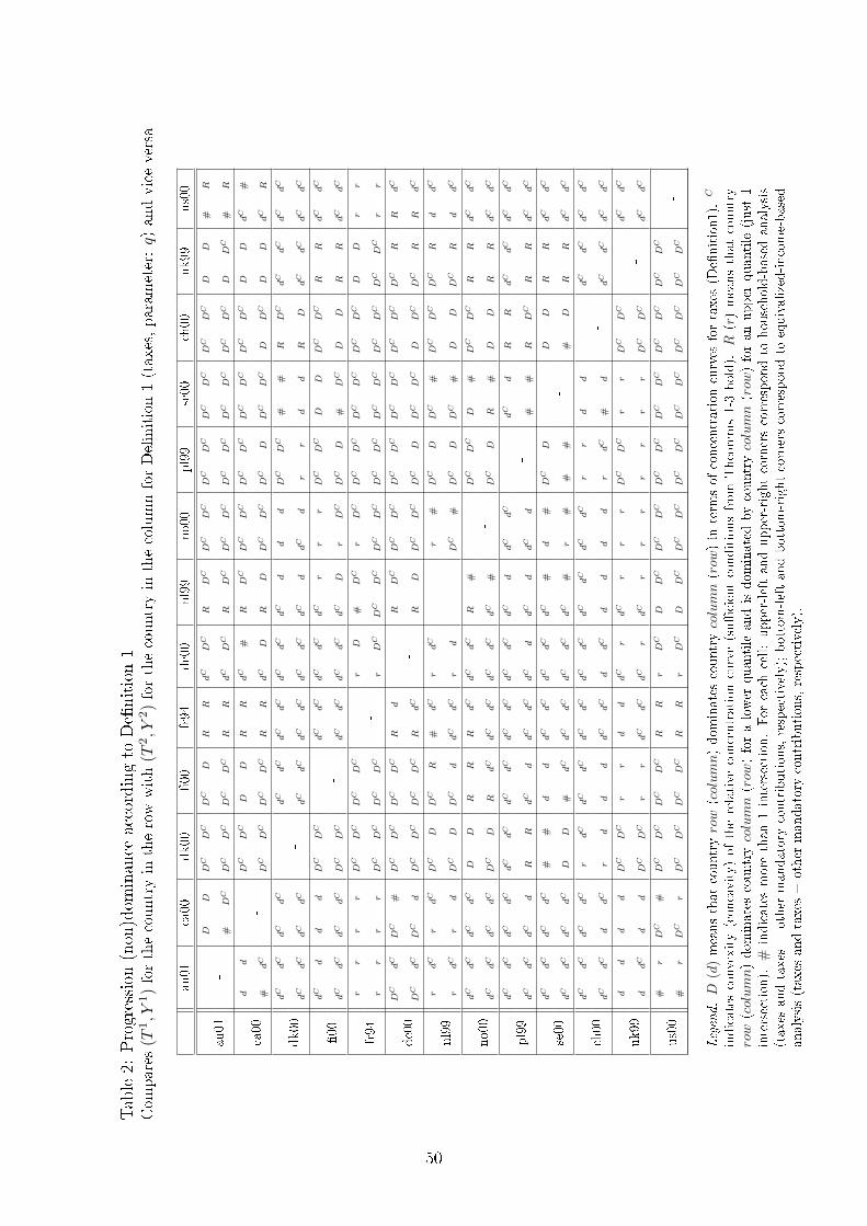
Table2:

Progression

(non)dom

inance

accordingto

De�nition1

Com

pares

(T1,Y

1)forthecountryin

therowwith

(T2,Y

2)forthecountryin

thecolumnforDe�nition1(taxes,param

eter:q)

andviceversa

au01

ca00

dk00

�00

fr94

de00

nl99

no00

pl99

se00

ch00

uk99

us00

DD

DC

DC

DC

DR

RdC

DC

RDC

DC

DC

DC

DC

DC

DC

DC

DC

DD

#R

au01

-#

DC

DC

DC

DC

DC

RR

dC

DC

RDC

DC

DC

DC

DC

DC

DC

DC

DC

DDC

#R

dd

DC

DC

DD

RR

dC

#R

DC

DC

DC

DC

DC

DC

DC

DC

DC

DD

dC

#

ca00

#dC

-DC

DC

DC

DC

RR

dC

DR

DDC

DC

DC

DDC

DC

DDC

DD

dC

R

dC

dC

dC

dC

dC

dC

dC

dC

dC

dC

dC

dd

dDC

DC

##

RDC

dC

dC

dC

dC

dk00

dC

dC

dC

dC

-dC

dC

dC

dC

dC

dC

dC

ddC

dr

rd

dR

DdC

dC

dC

dC

dC

dd

dDC

DC

dC

dC

dC

dC

dC

rr

rDC

DC

DD

DC

DC

RR

dC

dC

�00

dC

dC

dC

dC

DC

DC

-dC

dC

dC

dC

dC

Dr

DC

DC

D#

DC

DD

RR

dC

dC

rr

rr

DC

DC

DC

DC

rD

#DC

rDC

DC

DC

DC

DC

DC

DC

DD

rr

fr94

rr

rr

DC

DC

DC

DC

-r

DC

DC

DC

DC

DC

DC

DC

DC

DC

DC

DC

DC

DC

rr

DC

dC

DC

#DC

DC

DC

DC

Rd

RDC

DC

DC

DC

DC

DC

DC

DC

DC

DC

RR

dC

de00

DC

dC

DC

dDC

DC

DC

DC

RdC

-R

DDC

DC

DC

DDC

DC

DDC

DC

RR

dC

rdC

rdC

DC

DDC

R#

dC

rdC

r#

DC

DDC

#DC

DC

DC

Rd

dC

nl99

rdC

rd

DC

DDC

ddC

dC

rd

-DC

#DC

DDC

#D

DDC

Rd

dC

dC

dC

dC

dC

DD

RR

RdC

dC

dC

R#

DC

DC

D#

DC

DC

RR

dC

dC

no00

dC

dC

dC

dC

DC

DR

dC

dC

dC

dC

dC

dC

#-

DC

DR

#D

DR

RdC

dC

dC

dC

dC

dC

dC

dC

dC

dC

dC

dC

dC

dC

dC

ddC

dC

dC

dR

RdC

dC

dC

dC

pl99

dC

dC

dC

dR

RdC

ddC

dC

dC

ddC

ddC

d-

##

RDC

RR

dC

dC

dC

dC

dC

dC

##

dd

dC

dC

dC

dC

dC

#d

#DC

DD

DR

RdC

dC

se00

dC

dC

dC

dC

DD

#dC

dC

dC

dC

dC

dC

#r

##

#-

#D

RR

dC

dC

dC

dC

dC

dC

rdC

dC

dC

dC

dC

dC

dC

dC

dC

dC

dC

rr

dd

dC

dC

dC

dC

ch00

dC

dC

ddC

rd

dd

dC

dC

ddC

dd

dd

rdC

#d

-dC

dC

dC

dC

dd

dd

DC

DC

rr

dd

dC

rdC

rr

rDC

DC

rr

DC

DC

dC

dC

uk99

ddC

dd

DC

DC

rr

dC

dC

dC

rdC

rr

rr

rr

rDC

DC

-dC

dC

#r

DC

#DC

DC

DC

DC

RR

rDC

DDC

DC

DC

DC

DC

DC

DC

DC

DC

DC

DC

us00

#r

DC

rDC

DC

DC

DC

RR

rDC

DDC

DC

DC

DC

DC

DC

DC

DC

DC

DC

DC

-

Legen

d.D

(d)meansthat

countryrow(column)dom

inates

countrycolumn(row

)in

term

sof

concentrationcurves

fortaxes

(De�nition1).C

indicates

convexity(concavity)of

therelative

concentrationcurve(su�cientconditionsfrom

Theorems1-3hold).

R(r)meansthat

country

row

(column)dom

inates

countrycolumn(row

)foralower

quantileandisdom

inated

bycountrycolumn(row

)foran

upper

quantile(just

1intersection).

#indicates

morethan

1intersection.For

each

cell:upper-leftandupper-rightcornerscorrespondto

household-based

analysis

(taxes

andtaxes

+other

mandatorycontributions,respectively);bottom-leftandbottom-rightcornerscorrespondto

equivalized-income-based

analysis(taxes

andtaxes

+other

mandatorycontributions,respectively).

50

Table3:

Progression

(non)dom

inance

accordingto

De�nition2

Com

pares

(T1,Y

1)forthecountryin

therowwith

(T2,Y

2)forthecountryin

thecolumnforDe�nition2(taxes,param

eter:p)andviceversa

au01

ca00

dk00

�00

fr94

de00

nl99

no00

pl99

se00

ch00

uk99

us00

RD

DC

DC

DC

DR

RdC

DR

DDC

DD

DDC

DC

DD

DDC

#D

au01

-R

DC

DD

DD

RR

dC

DR

DD

DDC

DC

DC

DC

DC

DC

DC

DC

#D

rd

DC

DC

DD

dC

dC

dC

#R

DD

DD

DDC

DC

DD

DD

r#

ca00

rdC

-DC

DC

DD

dC

dC

dC

#R

DD

DD

DDC

DC

DDC

DD

r#

dC

dC

dC

dC

dC

rdC

dC

dC

dC

dC

dr

rD

D#

rR

Dr

rdC

dC

dk00

dd

dC

dC

-dC

rdC

dC

dC

rdC

dr

rr

rd

rR

Dr

rdC

dC

dC

dd

dDC

RdC

dC

dC

ddC

dD

DD

DR

RR

DC

##

dC

dC

�00

dd

dd

DC

R-

ddC

dC

ddC

#D

DDC

DC

RR

RDC

D#

dC

dC

rr

DC

DC

DC

DC

DC

DC

rDC

#DC

DC

DC

DC

DC

DC

DC

DC

DC

DC

DC

#D

fr94

rr

DC

DC

DC

DC

DDC

-r

DC

DD

DDC

DC

DC

DC

DC

DC

DC

DC

DC

DC

DC

DC

dDC

#DC

DC

DC

DR

dC

RR

DC

DC

DC

DC

DC

DC

DD

DC

DC

D#

de00

DC

dDC

#DC

RDC

DR

dC

-R

RDC

DDC

DDC

RDC

DC

DC

DC

DR

rd

rd

DC

DDC

D#

dC

rr

DC

DD

DDC

DDC

DC

DC

#r

r

nl99

rd

rd

DC

DDC

#d

dr

r-

DC

DC

DC

DDC

DDC

DC

DC

#r

r

dC

dd

dR

Rd

ddC

dC

dC

dC

dC

dDC

DR

#R

RR

RdC

dC

no00

dd

dd

RR

dd

ddC

dC

ddC

dC

-DC

DC

RR

RR

#R

dC

dC

dd

dd

dd

dd

dC

dC

dC

dC

dd

dC

dd

d#

#d

ddC

dC

pl99

dC

dC

dd

RR

dC

dC

dC

dC

dC

ddC

ddC

dC

-d

#R

RdC

ddC

dC

dC

dC

dC

dC

#R

rr

dC

dC

dC

dC

dC

dr

#D

D#

D#

#dC

dC

se00

dC

dC

dC

dC

DR

rr

dC

dC

dC

rdC

dr

rD

#-

#D

#r

dC

dC

dd

dd

rd

rdC

dC

dC

dd

dC

dC

rr

##

#d

rdC

dC

dC

ch00

dC

dC

ddC

rd

rdC

dC

dC

dC

dC

dC

dC

rr

rr

#d

-r

dC

dC

dC

ddC

dd

RR

##

dC

dC

dC

dC

dC

#r

rD

D#

#R

DC

dC

dC

uk99

dC

dC

dd

RR

d#

dC

dC

dC

dC

dC

##

rDC

D#

RR

DC

-dC

dC

#d

R#

DC

DC

DC

DC

#d

d#

RR

DC

DC

DC

DC

DC

DC

DC

DC

DC

DC

us00

#d

R#

DC

DC

DC

DC

dC

dC

dr

RR

DC

DC

DC

DC

DC

DC

DC

DC

DC

DC

-

Legen

d.D

(d)meansthat

countryrow

(column)dom

inates

countrycolumn(row

)in

term

sof

concentrationcurves

fortaxes,based

ongross

incomesharecumulants(D

e�nition2).Cindicates

convexity(concavity)of

therelative

concentrationcurve(su�cientconditionsfrom

Theorems

1-3hold).R

(r)meansthat

countryrow(column)dom

inates

countrycolumn(row

)foralower

quantileandisdom

inated

bycountrycolumn

(row

)foran

upper

quantile

(just

1intersection).

#indicates

morethan

1intersection.

For

each

cell:upper-leftandupper-rightcorners

correspondto

household-based

analysis(taxes

andtaxes

+other

mandatorycontributions,respectively);bottom-leftandbottom-rightcorners

correspondto

equivalized-income-based

analysis(taxes

andtaxes

+other

mandatorycontributions,respectively).

51

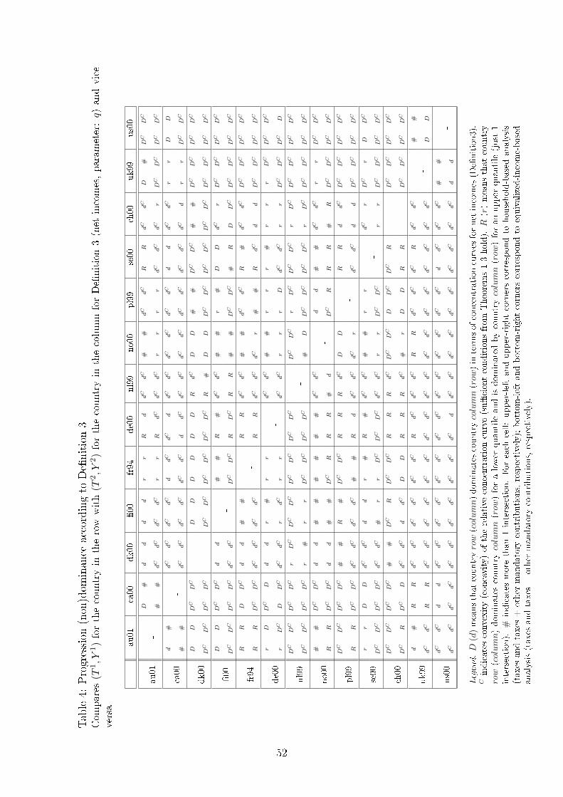
Table4:

Progression

(non)dom

inance

accordingto

De�nition3

Com

pares

(T1,Y

1)forthecountryin

therowwith

(T2,Y

2)forthecountryin

thecolumnforDe�nition3(net

incomes,param

eter:q)

andvice

versa

au01

ca00

dk00

�00

fr94

de00

nl99

no00

pl99

se00

ch00

uk99

us00

D#

dd

dd

rr

Rd

dC

dC

##

dC

dC

RR

dC

dC

D#

DC

DC

au01

-#

#dC

dC

dC

dC

rr

RdC

dC

dC

rr

rr

dC

dC

dC

rDC

DC

DC

DC

d#

dC

dC

dC

dC

ddC

dC

ddC

dC

dC

dC

dC

dC

dd

dC

dC

rr

DD

ca00

##

-dC

dC

dC

dC

dC

dC

ddC

dC

dC

dC

dC

dC

dC

dC

dC

dC

dr

rDC

DC

DD

DC

DC

DD

DD

DD

RdC

DD

##

DC

DC

##

DC

DC

DC

DC

dk00

DC

DC

DC

DC

-DC

DC

DC

DC

DC

DC

R#

DD

DC

DC

DC

DC

DC

DC

DC

DC

DC

DC

DD

DC

DC

dd

##

R#

dC

dC

##

r#

DD

dC

rDC

DC

DC

DC

�00

DC

DC

DC

DC

dC

dC

-DC

DC

RDC

RR

##

DC

DC

#R

DDC

DC

DC

DC

DC

RR

DDC

dd

##

RR

dC

dC

##

dC

dC

R#

dC

dC

DC

DC

DC

DC

fr94

RR

DC

DC

dC

dC

dC

dC

-R

RdC

dC

dC

r#

#R

dC

dd

DC

DC

DC

DC

rD

DC

Dd

dr

#r

rdC

dC

##

rr

r#

rr

rDC

DC

DC

de00

rDC

DDC

dC

dC

rdC

rr

-dC

dC

rr

rD

dC

dC

rr

DC

DC

DC

D

DC

DC

DC

DC

rDC

DC

DC

DC

DC

DC

DC

DC

DC

rDC

DC

DC

rDC

DC

DC

DC

DC

nl99

DC

DC

DC

DC

r#

rr

DC

DC

DC

DC

-#

DDC

DC

DC

DC

rDC

DC

DC

DC

DC

##

DC

DC

dd

##

##

##

dC

dC

dd

##

dC

dC

rr

DC

DC

no00

RR

DC

DC

dd

##

DC

RR

R#

d-

DC

RR

R#

RDC

DC

DC

DC

DC

DC

DC

DC

##

R#

DC

DC

RR

RdC

DD

RR

ddC

DC

DC

DC

DC

pl99

RR

DC

DC

dC

dC

dC

dC

##

Rd

dC

dC

dC

r-

dC

dC

dd

DC

DC

DC

DC

rr

DD

dC

dC

dd

r#

R#

dC

dC

##

rr

dC

rDC

rD

DC

se00

DC

DC

DC

DC

dC

dC

#r

rDC

DC

DC

dC

dC

rr

DC

DC

-r

rDC

DC

DC

DC

DC

DC

DC

DC

##

DC

RDC

DC

RR

RdC

DC

DC

DDC

DC

RDC

DC

DC

DC

ch00

DC

RDC

DdC

dC

ddC

DD

RR

RdC

#r

DD

RR

-DC

DC

DC

DC

d#

RR

dC

dC

dC

dC

dC

dC

RdC

dC

dC

RR

dC

dC

dC

RdC

dC

##

uk99

dC

dC

RR

dC

dC

dC

dC

dC

dC

dC

dC

dC

dC

dC

dC

dC

dC

dC

dC

dC

dC

-D

D

dC

dC

dd

dC

dC

dC

dC

dC

dC

dC

dC

dC

dC

dC

dC

dC

dC

ddC

dC

dC

##

us00

dC

dC

dC

dC

dC

dC

dC

dC

dC

dC

dC

ddC

dC

dC

dC

dC

dC

dC

dC

dC

dC

dd

-

Legen

d.D

(d)meansthat

countryrow(column)dom

inates

countrycolumn(row

)in

term

sofconcentrationcurves

fornet

incomes

(De�nition3).

Cindicates

convexity(concavity)of

therelative

concentrationcurve(su�cientconditionsfrom

Theorems1-3hold).R

(r)meansthat

country

row

(column)dom

inates

countrycolumn(row

)foralower

quantileandisdom

inated

bycountrycolumn(row

)foran

upper

quantile(just

1intersection).

#indicates

morethan

1intersection.For

each

cell:upper-leftandupper-rightcornerscorrespondto

household-based

analysis

(taxes

andtaxes

+other

mandatorycontributions,respectively);bottom-leftandbottom-rightcornerscorrespondto

equivalized-income-based

analysis(taxes

andtaxes

+other

mandatorycontributions,respectively).

52

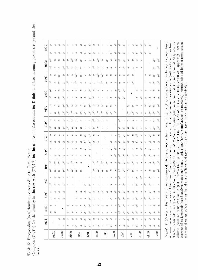
Table5:

Progression

(non)dom

inance

accordingto

De�nition4

Com

pares

(T1,Y

1)forthecountryin

therowwith

(T2,Y

2)forthecountryin

thecolumnforDe�nition4(net

incomes,param

eter:p)andvice

versa

au01

ca00

dk00

�00

fr94

de00

nl99

no00

pl99

se00

ch00

uk99

us00

R#

DD

DC

rDC

DC

Rr

RD

DC

DD

DDC

DC

DC

DDC

DC

##

au01

-R

rR

#D

#DC

DC

#r

RD

DD

DD

Rr

DD

DD

##

r#

D#

D#

DC

DC

#r

R#

DD

DC

DC

DC

DDC

DC

DD

##

ca00

rR

-#

RD

rDC

DC

#r

R#

DD

DC

DC

DC

DD

DDC

D#

#

dd

d#

rr

DD

dr

R#

DC

rDC

DC

rr

DC

DDC

Dr

r

dk00

r#

#r

-r

rDC

DC

Rr

R#

DDC

DC

DC

rr

DD

DC

DC

rr

dC

Rd

#R

RDC

RR

dR

RD

DD

DC

RR

DC

DC

DC

DR

R

�00

d#

dR

RR

-DC

RR

dR

RD

DDC

DR

RD

DC

DC

DC

RR

dC

dC

dC

dC

dd

dC

rd

dC

dC

dC

rr

DC

DC

dd

Dr

rr

dC

dC

fr94

dC

dC

dC

dC

dC

dC

dC

r-

dC

dC

dC

dC

rr

DC

DC

dC

dC

DD

rr

dC

dC

rR

#R

DR

rD

DDC

RR

DDC

DC

DDC

RD

DDC

D#

R

de00

#R

#R

rR

rD

DC

DC

-R

RDC

DC

DC

DC

rR

DDC

DC

DC

rR

rd

r#

r#

rr

DC

DC

rr

rD

DC

DC

rr

DC

DC

DD

rr

nl99

rd

r#

r#

rr

DC

DC

rr

-r

DDC

DC

rr

DC

D#

DC

rr

dC

dd

ddC

Rd

dR

Rd

dC

Rd

DC

DC

dd

RR

##

dC

dC

no00

dd

dd

ddC

dd

RR

dC

dC

Rd

-DC

Rd

#R

RR

RdC

dC

dd

dC

dC

dC

dC

ddC

dC

dC

dC

ddC

dC

dC

dC

dC

dC

##

ddC

dC

dC

pl99

dd

dC

dC

dC

dC

dC

ddC

dC

dC

dC

dC

dC

dC

r-

dC

dC

RR

dC

dC

dC

dC

dC

dC

dC

dR

Rr

rD

DdC

rR

RD

DDC

DC

DD

##

rr

se00

rR

dC

dR

Rr

rDC

DC

Rr

RR

D#

DC

DC

-DC

DD

D#

#

dC

ddC

dC

dC

ddC

dC

dR

dd

dC

dC

rr

##

dd

dd

dC

dC

ch00

dd

dd

dd

ddC

dd

ddC

dC

dr

rr

rdC

d-

dd

dC

dC

dC

dC

dd

dC

ddC

dR

RdC

dd

d#

#D

DC

##

DD

dC

dC

uk99

dd

dC

ddC

dC

dC

dC

RR

dC

dC

#dC

rr

DC

DC

dd

DD

-dC

dC

##

##

RR

rr

DC

DC

#r

RR

DC

DC

DC

DC

RR

DC

DC

DC

DC

us00

##

##

RR

rr

DC

DC

Rr

RR

DC

DC

DC

DC

##

DC

DC

DC

DC

-

Legen

d.D

(d)meansthat

countryrow

(column)dom

inates

countrycolumn(row

)in

term

sof

concentrationcurves

fornet

incomes,based

ongrossincomesharecumulants

(De�nition4).Cindicates

convexity(concavity)of

therelative

concentrationcurve(su�cientconditionsfrom

Theorems1-3hold).R(r)meansthat

countryrow(column)dom

inates

countrycolumn(row

)foralower

quantileandisdom

inated

bycountry

column(row

)foran

upper

quantile(just1intersection).

#indicates

morethan

1intersection.For

each

cell:upper-leftandupper-rightcorners

correspondto

household-based

analysis(taxes

andtaxes

+other

mandatorycontributions,respectively);bottom-leftandbottom-rightcorners

correspondto

equivalized-income-based

analysis(taxes

andtaxes

+other

mandatorycontributions,respectively).

53

Table6:

Progression

(non)dom

inance

accordingto

De�nition5

Com

pares

(T1,Y

1)forthecountryin

therowwith

(T2,Y

2)forthecountryin

thecolumnforDe�nition5(di�erencesof

taxconcentrationcurves,

param

eter:q)

andviceversa

au01

ca00

dk00

�00

fr94

de00

nl99

no00

pl99

se00

ch00

uk99

us00

DDC

DC

DC

DC

Dd

dR

DC

dr

DC

DDC

DC

DC

DC

DC

DDC

DC

RD

au01

-D

DC

DC

DC

rr

dC

dC

dC

DC

dC

Dr

DC

DC

DC

DC

DC

DDC

DC

DC

R#

ddC

DC

DC

rr

dC

dC

dC

rdC

rr

rDC

DC

DC

DC

DC

DC

DC

DR

R

ca00

ddC

-DC

Dr

rdC

dC

dC

rdC

rr

rDC

DC

rr

DD

DC

DR

R

dC

dC

dC

dC

dd

dC

dC

dC

dC

dC

ddC

rD

D#

#R

DC

RR

dC

dC

dk00

dC

dC

dC

d-

dC

dC

dC

dC

dC

dC

dC

ddC

rr

DC

##

RD

RR

RR

dC

dR

RD

DdC

dC

RR

dC

dD

DDC

DC

DC

DDC

DC

R#

RR

�00

RR

RR

DC

DC

-dC

dC

RR

dC

RD

DDC

DR

DC

DDC

RD

RR

DD

DC

DC

DC

DC

DC

DC

#DC

#DC

DC

DC

DC

DC

DC

DC

DC

DC

DC

DC

DDC

fr94

DC

DC

DC

DC

DC

DC

DC

DC

-D

DC

DDC

DC

DC

DC

DC

DC

DC

DC

DC

DC

DC

DC

DC

rdC

DC

RDC

DC

rr

#dC

##

DC

DC

DC

DDC

DC

DC

DDC

DC

RR

de00

DC

dC

DC

RDC

DC

rr

ddC

-#

#r

rDC

DDC

DC

DDC

DC

DR

R

DR

DC

RDC

DDC

D#

dC

##

DC

DDC

DC

DC

DDC

DC

DC

DD

R

nl99

DC

dDC

RDC

DDC

rd

dC

##

-DC

DDC

DDC

DC

DC

DDC

DD

R

dC

dR

RDC

Rd

ddC

dC

dC

dC

dC

dDC

DR

#DC

DC

RR

RR

no00

RdC

RR

DC

Rd

ddC

dC

RR

dC

d-

DC

DR

RR

DR

RR

R

dC

dC

dC

dC

dd

dC

dC

dC

dC

dC

ddC

dC

dC

dd

d#

#R

RdC

dC

pl99

dC

dC

dC

dC

RdC

dC

ddC

dC

dC

ddC

ddC

d-

d#

#DC

RR

RR

dC

dC

dC

dC

##

dC

ddC

dC

dC

dC

dC

dr

#D

DD

DC

RR

RR

se00

dC

dC

RR

##

rdC

dC

dC

dC

dC

dC

dC

rr

D#

-#

DR

#R

R

dC

ddC

dC

rdC

dC

dC

dC

dC

dC

ddC

dC

dC

dC

##

ddC

Rd

dC

dC

ch00

ddC

dd

rd

ddC

dC

dC

ddC

dC

dr

d#

dC

#d

-d

dC

dC

dC

dC

dC

dC

dr

rr

#dC

dC

dC

dC

dC

dr

rr

rr

rr

DdC

dC

uk99

dC

dC

dC

dr

rr

ddC

dC

dC

ddC

dr

rr

rr

#D

DC

-dC

dC

rd

rr

DC

DC

rr

ddC

rr

dr

rr

DC

DC

rr

DC

DC

DC

DC

us00

r#

rr

rr

rr

dC

dC

rr

dr

rr

rr

rr

DC

DC

DC

DC

-

Legen

d.D

(d)meansthat

countryrow(column)dom

inates

countrycolumn(row

)interm

sofsecond-orderdi�erencesofconcentrationcurves

for

grossincomes

andtaxes

(De�nition5).Cindicates

convexity(concavity)of

therelative

concentrationcurve(su�cientconditionsfrom

Theorems

1-3hold).R

(r)meansthat

countryrow(column)dom

inates

countrycolumn(row

)foralower

quantileandisdom

inated

bycountrycolumn

(row

)foran

upper

quantile

(just

1intersection).

#indicates

morethan

1intersection.

For

each

cell:upper-leftandupper-rightcorners

correspondto

household-based

analysis(taxes

andtaxes

+other

mandatorycontributions,respectively);bottom-leftandbottom-rightcorners

correspondto

equivalized-income-based

analysis(taxes

andtaxes

+other

mandatorycontributions,respectively).

54

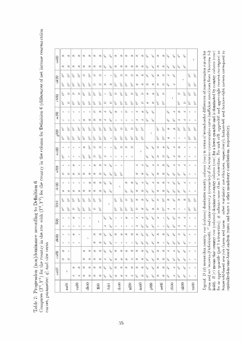
Table7:

Progression

(non)dom

inance

accordingto

De�nition6

Com

pares

(T1,Y

1)forthecountryin

therowwith

(T2,Y

2)forthecountryin

thecolumnforDe�nition6(di�erencesof

net

incomeconcentration

curves,param

eter:q)

andviceversa

au01

ca00

dk00

�00

fr94

de00

nl99

no00

pl99

se00

ch00

uk99

us00

D#

rr

rr

DC

DC

#r

Dr

DC

rDC

DC

rr

DC

DC

DC

DC

RR

au01

-D

rr

rr

rDC

DC

#r

Dr

rr

DC

DC

rr

DD

DC

DC

RR

d#

r#

r#

DDC

#r

##

rr

DC

DC

rr

DC

DDC

DC

RR

ca00

dR

-r

rr

rDC

DC

#r

Dr

rr

DC

DC

rr

DC

DDC

DC

RR

RR

R#

rr

DC

DC

Rr

Rr

DC

#DC

DC

#r

DC

DC

DC

DR

R

dk00

RR

RR

-r

rDC

DC

R#

Rr

DC

DC

DC

DC

Rr

DC

DC

DC

DC

RR

RR

R#

RR

DDC

RR

R#

DD

DC

DC

RD

DC

DC

DD

RR

�00

RR

RR

RR

-DC

DC

RR

RR

DC

DDC

DC

RR

DC

DC

DD

RR

dC

dC

ddC

dC

dC

ddC

dC

dC

dC

dd

rDC

DC

dd

Dr

Rr

dC

dC

fr94

dC

dC

dC

dC

dC

dC

dC

dC

-dC

dC

dC

dC

rr

rDC

dC

dC

DDC

Rr

dC

dC

#R

#R

rR

rr

DC

DC

DC

rr

DC

DC

DC

r#

DC

DDC

DC

RR

de00

#R

#R

r#

rr

DC

DC

-DC

rr

DDC

Dr

rDC

DC

DC

DR

R

dR

##

rR

r#

DC

DdC

Rr

DDC

DC

rD

DC

DC

DC

DR

R

nl99

dR

dR

rR

rr

DC

DC

dC

R-

rD

DC

Dr

rDC

DDC

DR

R

dC

RR

RdC

#d

dD

RR

dC

Rd

DC

DC

dd

DC

DC

##

RR

no00

RR

RR

dC

dC

dC

dR

RR

dR

d-

DC

DC

d#

DD

RR

RR

dC

dC

dC

dC

dC

dC

dC

dC

dC

dC

dC

dC

dC

dC

dC

dC

dC

dC

##

RdC

dC

dC

pl99

dC

dC

dC

dC

dC

dC

dC

dC

RdC

dC

ddC

ddC

dC

-dC

dC

R#

RdC

dC

dC

RR

RR

#R

rd

DD

R#

Rd

DD

DC

DC

DC

DC

D#

RR

se00

RR

RR

rR

rr

DC

DC

RR

RR

D#

DC

DC

-DC

DD

DR

R

dC

dC

dC

ddC

dC

dC

dC

dR

dC

ddC

dC

dC

dC

##

dC

dC

dC

ddC

dC

ch00

dd

dC

ddC

dC

dC

dC

ddC

dC

dC

dC

dd

dr

#dC

d-

ddC

dC

dC

dC

dC

dC

dC

dC

dd

dr

RdC

dC

dC

d#

#r

DC

d#

DC

DdC

dC

uk99

dC

dC

dC

dC

dC

dC

dd

rR

dC

ddC

dr

rr

DC

dd

DDC

-dC

dC

rr

rr

rr

rr

DC

DC

rr

rr

rr

DC

DC

rr

DC

DC

DC

DC

us00

rr

rr

rr

rr

DC

DC

rr

rr

rr

DC

DC

rr

DC

DC

DC

DC

-

Legen

d.D

(d)meansthat

countryrow(column)dom

inates

countrycolumn(row

)interm

sofsecond-orderdi�erencesofconcentrationcurves

for

grossandnetincomes(D

e�nition6).Cindicatesconvexity(concavity)oftherelative

concentrationcurve(su�cientconditionsfrom

Theorems1-3

hold).R(r)meansthat

countryrow(column)dom

inates

countrycolumn(row

)foralower

quantileandisdom

inated

bycountrycolumn(row

)foran

upper

quantile(just1intersection).

#indicates

morethan

1intersection.For

each

cell:upper-leftandupper-rightcornerscorrespondto

household-based

analysis(taxes

andtaxes

+other

mandatorycontributions,respectively);bottom-leftandbottom-rightcornerscorrespondto

equivalized-income-based

analysis(taxes

andtaxes

+other

mandatorycontributions,respectively).

55

Table8:

Summarytaxprogression

statistics

forhouseholddata,

taxes

Progression,

Progression,

Singleextr.

Singleextr.,

Noprogression,

Noprogression,

Oneintersection,

Oneintersection,

#of

cases

%of

totalcases

%of

possible

#of

cases

%of

totalcases

#of

cases

%of

possible

De�nition1

5975.64

4983.05

1924.36

1684.21

De�nition2

5367.95

3769.81

2532.05

1768.00

De�nition3

5266.67

3771.15

2633.33

1765.38

De�nition4

5165.38

3160.78

2734.62

2074.07

De�nition5

5570.51

4581.82

2329.49

1878.26

De�nition6

4557.69

3475.56

3342.31

2781.82

Average

52.50

67.31

38.83

73.70

25.50

32.69

19.17

75.29

Total

cases

78

Table9:

Summarytaxprogression

statistics

forhouseholddata,

taxes+payroll

Progression,

Progression,

Singleextr.

Singleextr.,

Noprogression,

Noprogression,

Oneintersection,

Oneintersection,

#of

cases

%of

totalcases

%of

possible

#of

cases

%of

totalcases

#of

cases

%of

possible

De�nition1

6076.92

4778.33

1823.08

1266.67

De�nition2

6076.92

3050.00

1823.08

1055.56

De�nition3

5266.67

4076.92

2633.33

1142.31

De�nition4

4658.97

2350.00

3241.03

2268.75

De�nition5

5671.79

3664.29

2228.21

1777.27

De�nition6

4253.85

2969.05

3646.15

2672.22

Average

52.67

67.52

34.17

64.76

25.33

32.48

16.33

63.80

Total

cases

78

56

Table10:Summarytaxprogression

statistics

forequivalized

data,

taxes

Progression,

Progression,

Singleextr.

Singleextr.,

Noprogression,

Noprogression,

Oneintersection,

Oneintersection,

#of

cases

%of

totalcases

%of

possible

#of

cases

%of

totalcases

#of

cases

%of

possible

De�nition1

5671.79

4783.93

2228.21

1777.27

De�nition2

5671.79

4071.43

2228.21

1881.82

De�nition3

5671.79

5089.29

2228.21

1672.73

De�nition4

4658.97

2963.04

3241.03

2578.13

De�nition5

4962.82

3877.55

2937.18

2586.21

De�nition6

4355.13

3376.74

3544.87

3394.29

Average

51.00

65.38

39.50

77.00

27.00

34.62

22.33

81.74

Total

cases

78

Table11:Summarytaxprogression

statistics

forequivalized

data,

taxes+payroll

Progression,

Progression,

Singleextr.

Singleextr.,

Noprogression,

Noprogression,

Oneintersection,

Oneintersection,

#of

cases

%of

totalcases

%of

possible

#of

cases

%of

totalcases

#of

cases

%of

possible

De�nition1

6279.49

4470.97

1620.51

1275.00

De�nition2

5570.51

3360.00

2329.49

1773.91

De�nition3

5975.64

5186.44

1924.36

1578.95

De�nition4

4557.69

2657.78

3342.31

2575.76

De�nition5

5165.38

3364.71

2734.62

2281.48

De�nition6

4253.85

2866.67

3646.15

3391.67

Average

52.33

67.09

35.83

67.76

25.67

32.91

20.67

79.46

Total

cases

78

57

Table12:Summarystatistics:consistency

forstrict

dom

inance

Incidence

ofstrict

Householddata,

taxes

Householddata,

taxes+payroll

Equivalized

data,

taxes

Equivalized

data,

taxes+payroll

dom

inance

(outof

6)#

ofcases

%of

totalcases

#of

cases

%of

totalcases

#of

cases

%of

totalcases

#of

cases

%of

totalcases

62

2.56

22.56

56.41

78.97

520

25.64

2329.49

1417.95

1519.23

416

20.51

1114.10

810.26

911.54

319

24.36

2532.05

2937.18

2532.05

215

19.23

78.97

1620.51

1316.67

15

6.41

810.26

56.41

810.26

Table13:Summarystatistics:consistency

forbifurcatedom

inance

(oneconsistentintersection

isallowed)

Incidence

ofbifurcate

Householddata,

taxes

Householddata,

taxes+payroll

Equivalized

data,

taxes

Equivalized

data,

taxes+payroll

dom

inance

(outof

6)#

ofcases

%of

totalcases

#of

cases

%of

totalcases

#of

cases

%of

totalcases

#of

cases

%of

totalcases

64

5.13

45.13

810.26

1215.38

528

35.90

2937.18

2025.64

1924.36

423

29.49

1823.08

2126.92

2126.92

321

26.92

2228.21

2835.90

2633.33

20

0.00

45.13

11.28

00.00

12

2.56

11.28

00.00

00.00

58

Table 14: (Dis)Similarities among progression comparison concepts

De�nition 2 De�nition 3 De�nition 4 De�nition 5 De�nition 6

De�nition 1 83.66 13.46 20.51 78.52 63.46 35.26 65.06 33.02 49.36 50.00

De�nition 2 - 21.16 78.52 60.90 36.54 67.62 29.81 45.83 52.88

De�nition 3 . - 27.88 71.47 46.16 53.52 48.72 50.64

De�nition 4 . . - 51.92 47.12 69.23 26.60

De�nition 5 . . . - 58.97 40.06

Legend. The �rst [second] entry in a cell denotes the average percentage of similarity

[dissimilarity] between a pair of de�nitions. Symmetric entries are indicated by the dot

sign (.)

Table 15: US progression dominance for Bush sen., Clinton, and Bush jun.

91→94 94→00 00→04 91→04 91→00 94→04

Bsen → C* C* → C** C** → Bjun Bsen → Bjun Bsen → C** C* → Bjun

dC dC R # # # d d R d R #

Def. 1R dC R R dC r R R R R R R

d d # D # # # # # # # D

Def. 2r d # # r r # # # # # #

DC DC DC DC D D DC DC DC DC DC DC

Def. 3DC DC r r D D DC DC # D D DC

d d r r DC D # D r r D D

Def. 4d d r r DC D # # r r # D

R R D D R # R R R R # D

Def. 5R R # # R # R R R R # #

dC dC dC dC DC DC R R d dC D D

Def. 6dC dC dC dC D D R R dC dC # D

59

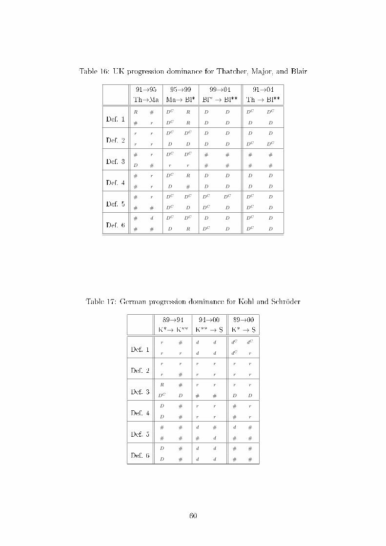
Table 16: UK progression dominance for Thatcher, Major, and Blair

91→95 95→99 99→04 91→04

Th→Ma Ma→ Bl* Bl* → Bl** Th → Bl**

R # DC R D D DC DC

Def. 1# r DC R D D D D

r r DC DC D D D D

Def. 2r r D D D D DC DC

# r DC DC # # # #

Def. 3D # r r # # # #

# r DC R D D D D

Def. 4# r D # D D D D

# r DC DC DC DC DC D

Def. 5# # DC D DC D DC D

# d DC DC D D DC D

Def. 6# # D R DC D DC D

Table 17: German progression dominance for Kohl and Schröder

89→94 94→00 89→00

K*→ K** K** → S K* → S

r # d d dC dC

Def. 1r r d d dC r

r r r r r r

Def. 2r # r r r r

R # r r r r

Def. 3DC D # # D D

D # r r # r

Def. 4D # r r # r

# # d # d #

Def. 5# # # d # #

D # d d # #

Def. 6D # d d # #

60

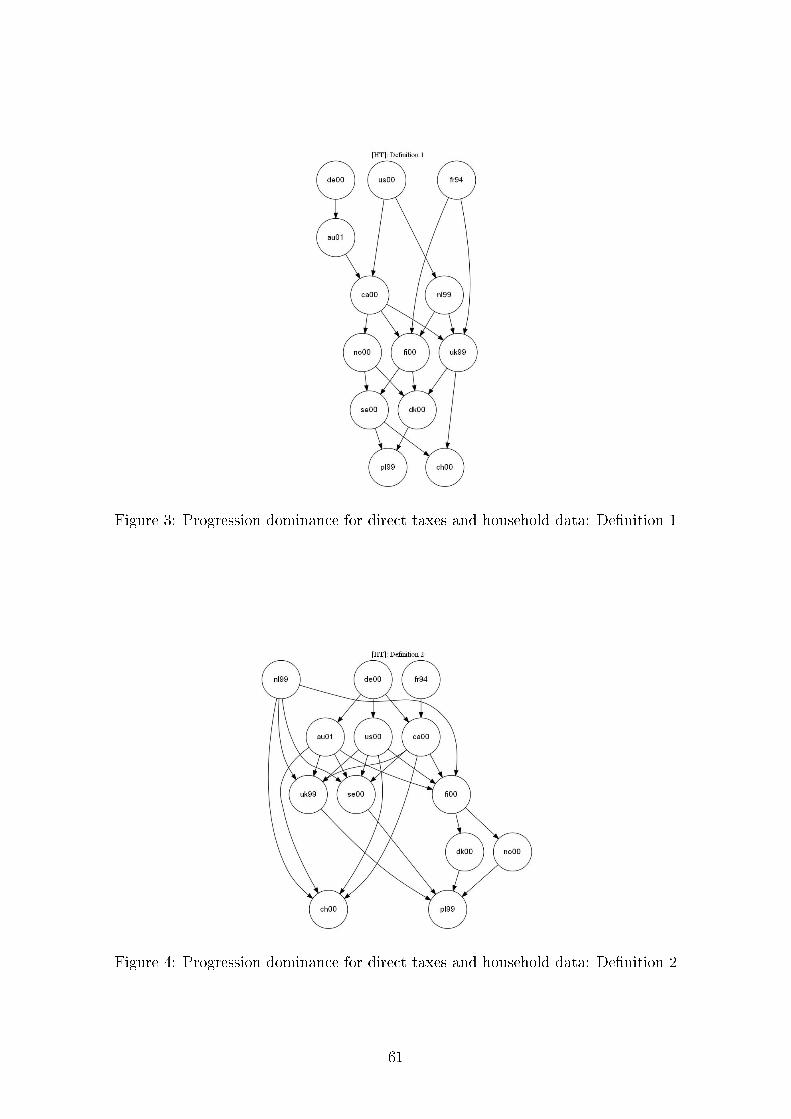
Figure 3: Progression dominance for direct taxes and household data: De�nition 1

Figure 4: Progression dominance for direct taxes and household data: De�nition 2

61

Figure 5: Progression dominance for direct taxes and household data: De�nition 3

Figure 6: Progression dominance for direct taxes and household data: De�nition 4

62

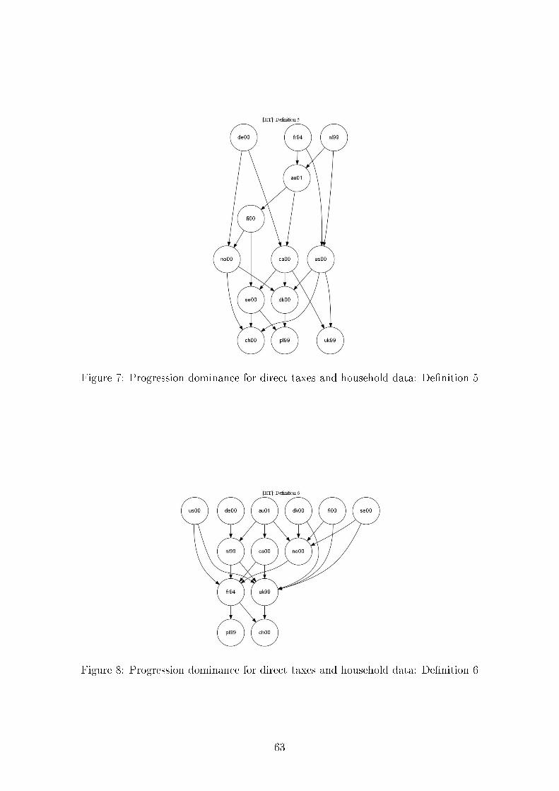
Figure 7: Progression dominance for direct taxes and household data: De�nition 5

Figure 8: Progression dominance for direct taxes and household data: De�nition 6

63

Figure 9: Progression dominance for direct and payroll taxes and household data: De�-

nition 1

Figure 10: Progression dominance for direct and payroll taxes and household data: Def-

inition 2

64

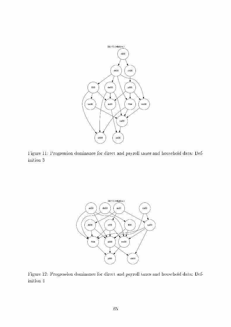
Figure 11: Progression dominance for direct and payroll taxes and household data: Def-

inition 3

Figure 12: Progression dominance for direct and payroll taxes and household data: Def-

inition 4

65

Figure 13: Progression dominance for direct and payroll taxes and household data: Def-

inition 5

Figure 14: Progression dominance for direct and payroll taxes and household data: Def-

inition 6

66

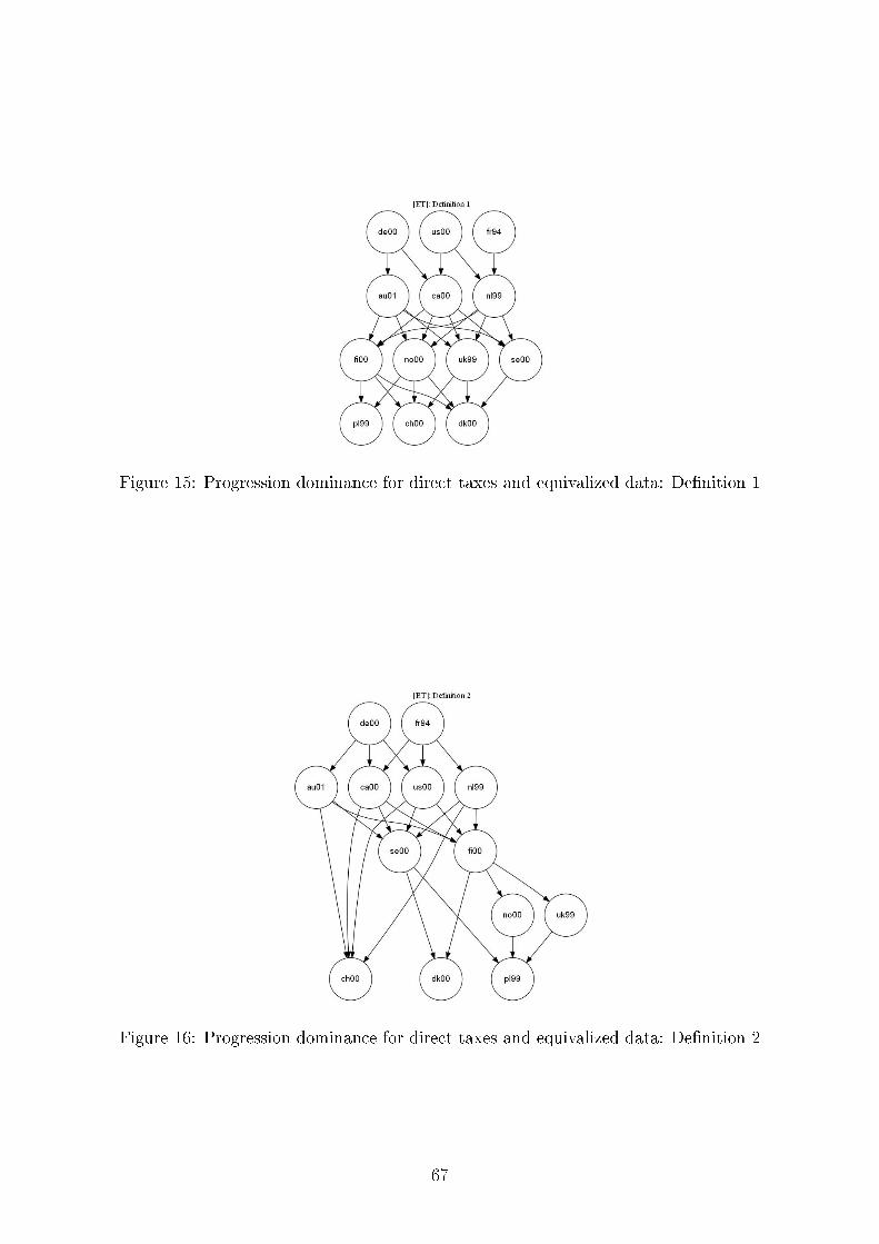
Figure 15: Progression dominance for direct taxes and equivalized data: De�nition 1

Figure 16: Progression dominance for direct taxes and equivalized data: De�nition 2

67

Figure 17: Progression dominance for direct taxes and equivalized data: De�nition 3

Figure 18: Progression dominance for direct taxes and equivalized data: De�nition 4

68

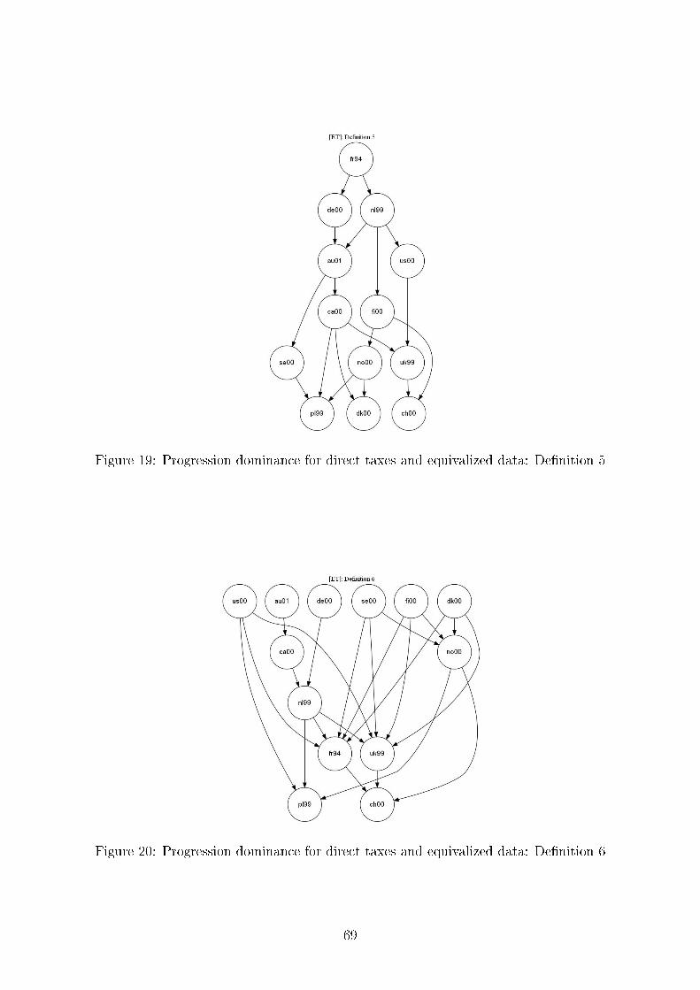
Figure 19: Progression dominance for direct taxes and equivalized data: De�nition 5

Figure 20: Progression dominance for direct taxes and equivalized data: De�nition 6

69

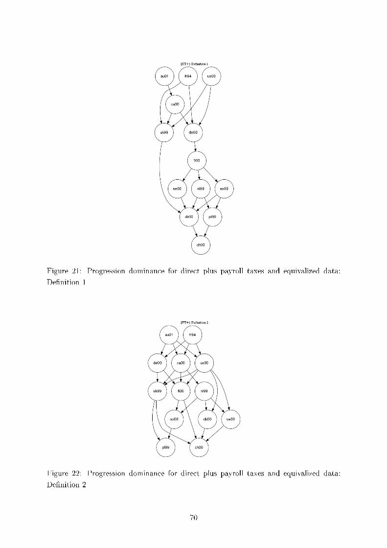
Figure 21: Progression dominance for direct plus payroll taxes and equivalized data:

De�nition 1

Figure 22: Progression dominance for direct plus payroll taxes and equivalized data:

De�nition 2

70

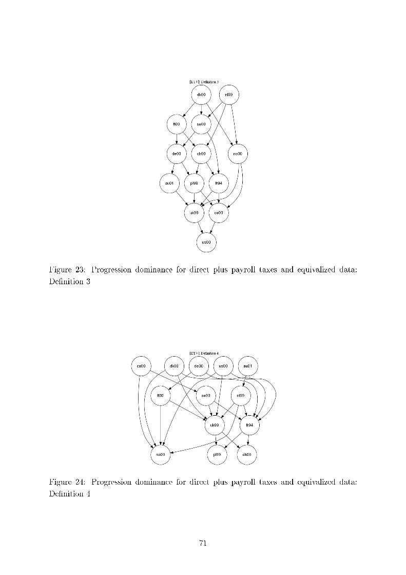
Figure 23: Progression dominance for direct plus payroll taxes and equivalized data:

De�nition 3

Figure 24: Progression dominance for direct plus payroll taxes and equivalized data:

De�nition 4

71

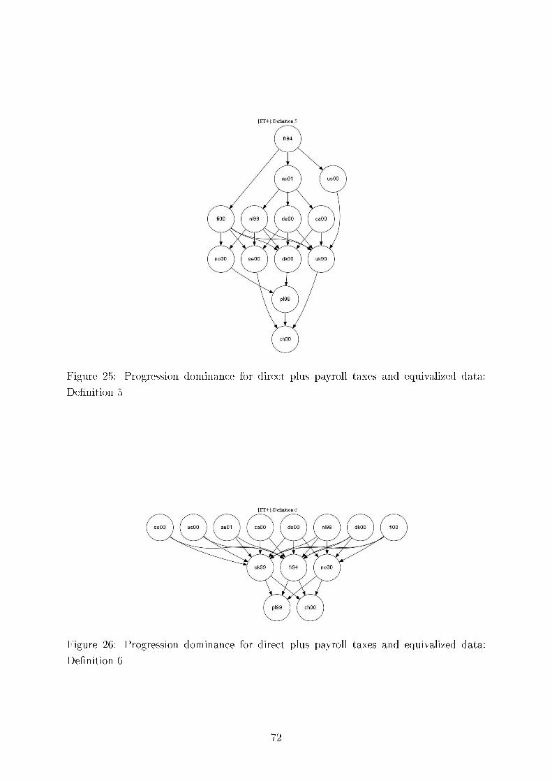
Figure 25: Progression dominance for direct plus payroll taxes and equivalized data:

De�nition 5

Figure 26: Progression dominance for direct plus payroll taxes and equivalized data:

De�nition 6

72

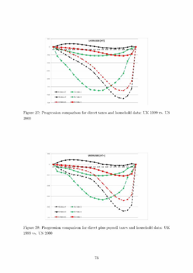
Figure 27: Progression comparison for direct taxes and household data: UK 1999 vs. US

2000

Figure 28: Progression comparison for direct plus payroll taxes and household data: UK

1999 vs. US 2000

73

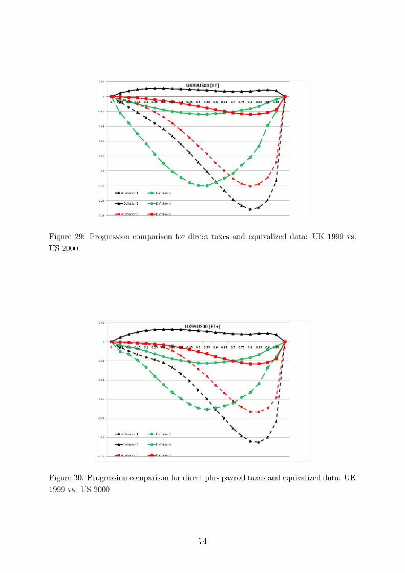
Figure 29: Progression comparison for direct taxes and equivalized data: UK 1999 vs.

US 2000

Figure 30: Progression comparison for direct plus payroll taxes and equivalized data: UK

1999 vs. US 2000

74

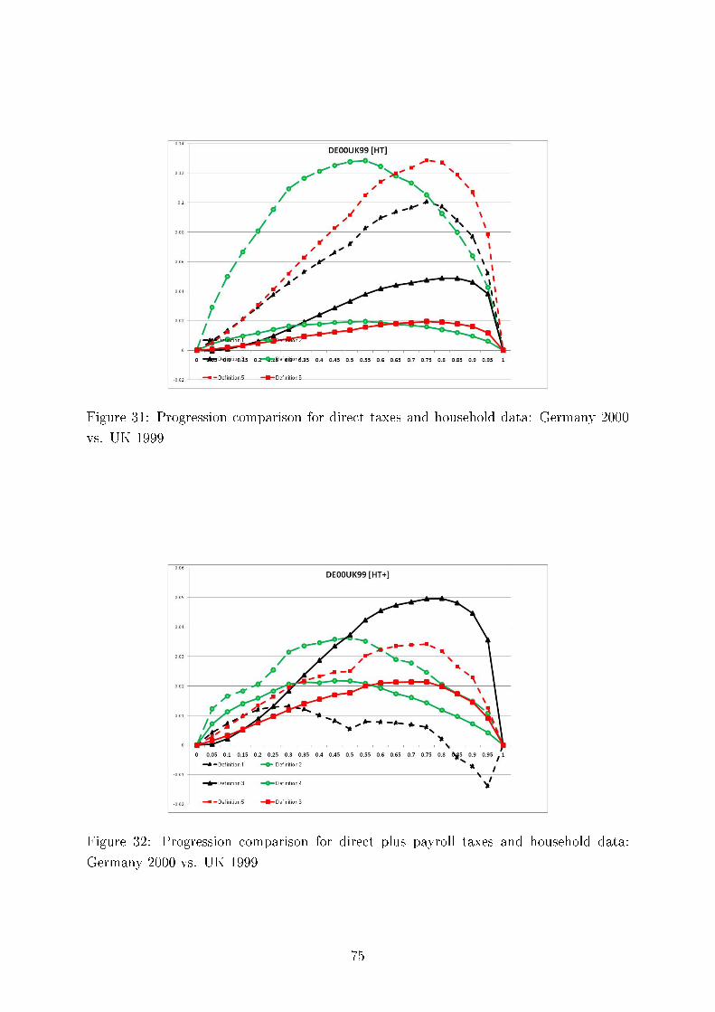
Figure 31: Progression comparison for direct taxes and household data: Germany 2000

vs. UK 1999

Figure 32: Progression comparison for direct plus payroll taxes and household data:

Germany 2000 vs. UK 1999

75

Figure 33: Progression comparison for direct taxes and equivalized data: Germany 2000

vs. UK 1999

Figure 34: Progression comparison for direct plus payroll taxes and equivalized data:

Germany 2000 vs. UK 1999

76

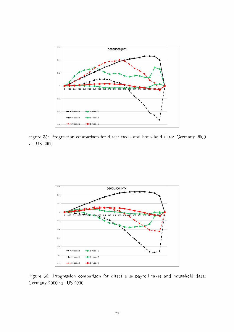
Figure 35: Progression comparison for direct taxes and household data: Germany 2000

vs. US 2000

Figure 36: Progression comparison for direct plus payroll taxes and household data:

Germany 2000 vs. US 2000

77

Figure 37: Progression comparison for direct taxes and equivalized data: Germany 2000

vs. US 2000

Figure 38: Progression comparison for direct plus payroll taxes and equivalized data:

Germany 2000 vs. US 2000

78

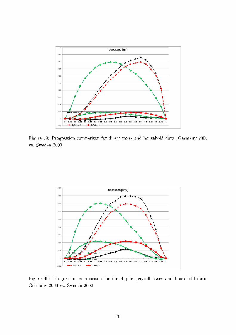
Figure 39: Progression comparison for direct taxes and household data: Germany 2000

vs. Sweden 2000

Figure 40: Progression comparison for direct plus payroll taxes and household data:

Germany 2000 vs. Sweden 2000

79

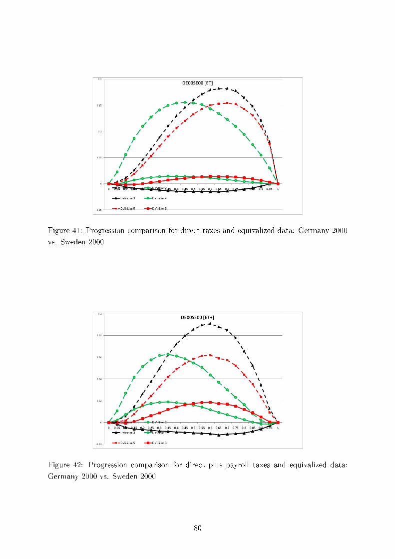
Figure 41: Progression comparison for direct taxes and equivalized data: Germany 2000

vs. Sweden 2000

Figure 42: Progression comparison for direct plus payroll taxes and equivalized data:

Germany 2000 vs. Sweden 2000

80

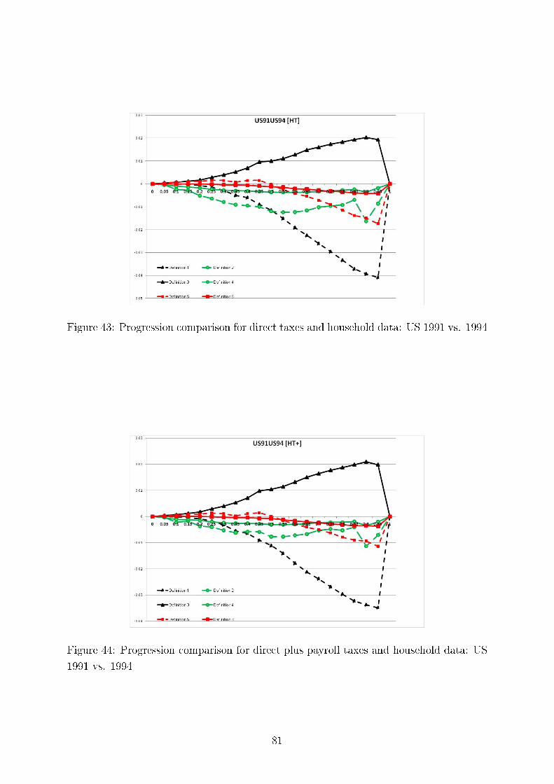
Figure 43: Progression comparison for direct taxes and household data: US 1991 vs. 1994

Figure 44: Progression comparison for direct plus payroll taxes and household data: US

1991 vs. 1994

81

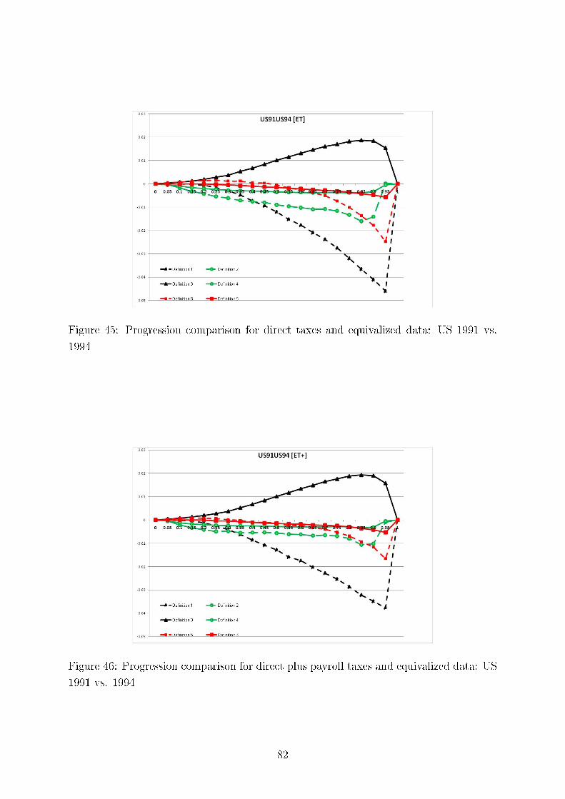
Figure 45: Progression comparison for direct taxes and equivalized data: US 1991 vs.

1994

Figure 46: Progression comparison for direct plus payroll taxes and equivalized data: US

1991 vs. 1994

82

Figure 47: Progression comparison for direct taxes and household data: US 1994 vs. 2000

Figure 48: Progression comparison for direct plus payroll taxes and household data: US

1994 vs. 2000

83

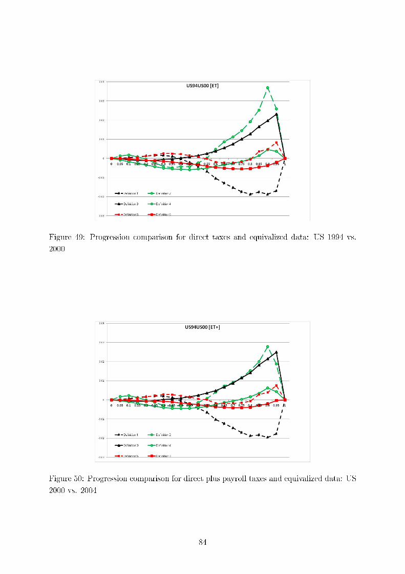
Figure 49: Progression comparison for direct taxes and equivalized data: US 1994 vs.

2000

Figure 50: Progression comparison for direct plus payroll taxes and equivalized data: US

2000 vs. 2004

84

Figure 51: Progression comparison for direct taxes and household data: US 2000 vs. 2004

Figure 52: Progression comparison for direct plus payroll taxes and household data: US

2000 vs. 2004

85

Figure 53: Progression comparison for direct taxes and equivalized data: US 2000 vs.

2004

Figure 54: Progression comparison for direct plus payroll taxes and equivalized data: US

2000 vs. 2004

86

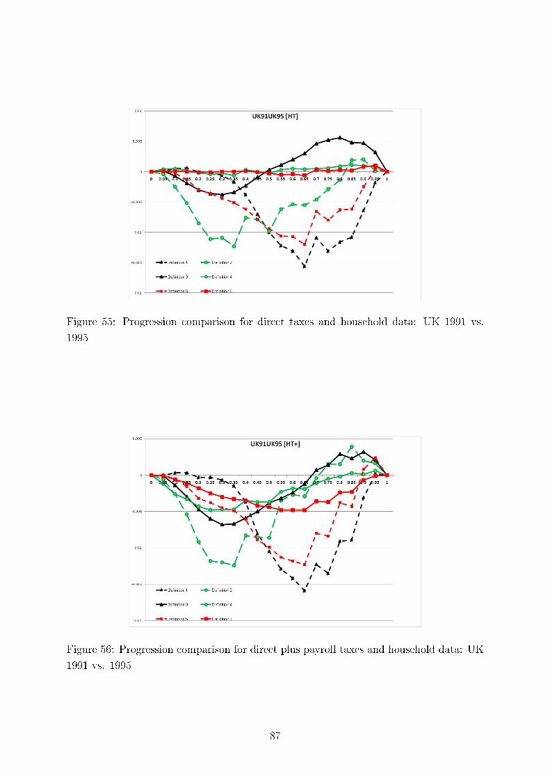
Figure 55: Progression comparison for direct taxes and household data: UK 1991 vs.

1995

Figure 56: Progression comparison for direct plus payroll taxes and household data: UK

1991 vs. 1995

87

Figure 57: Progression comparison for direct taxes and equivalized data: UK 1991 vs.

1995

Figure 58: Progression comparison for direct plus payroll taxes and equivalized data: UK

1991 vs. 1995

88

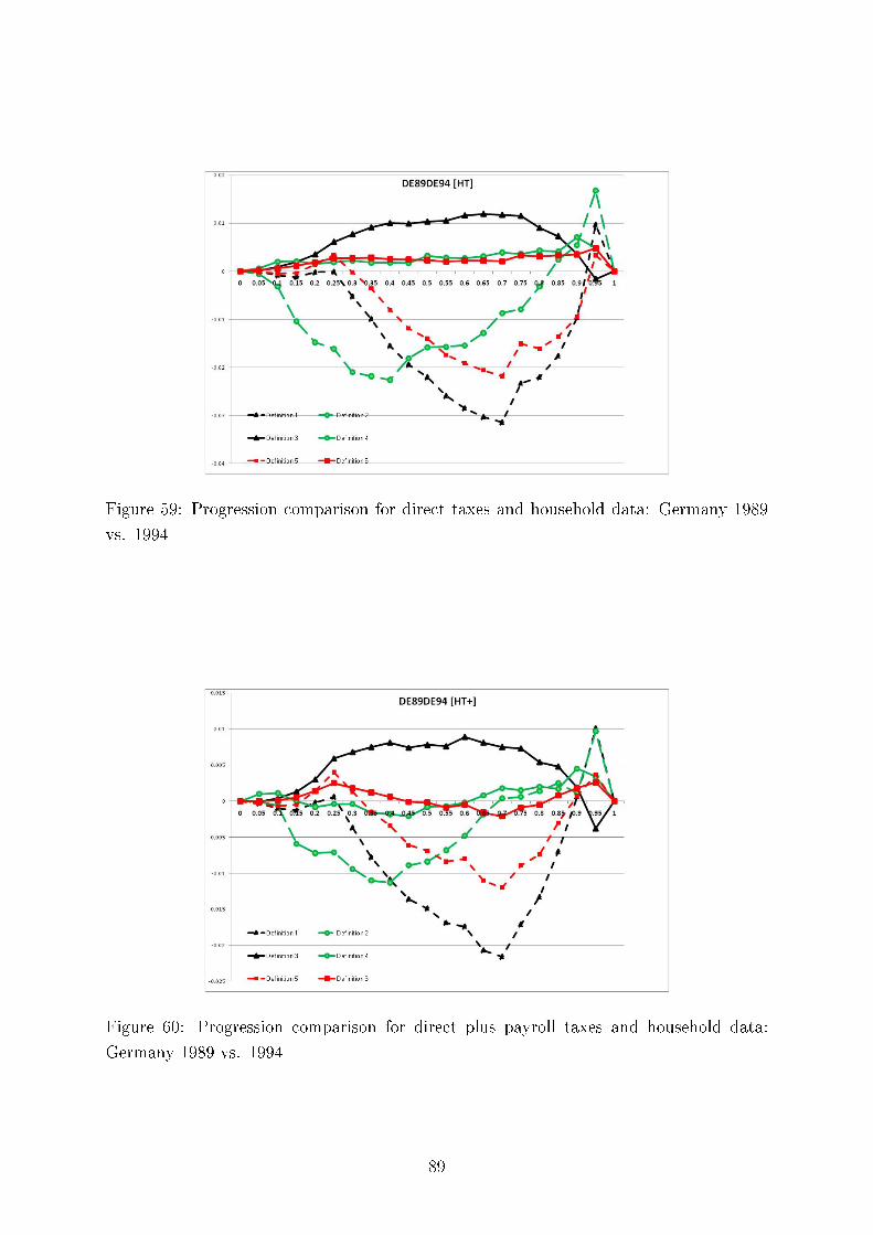
Figure 59: Progression comparison for direct taxes and household data: Germany 1989

vs. 1994

Figure 60: Progression comparison for direct plus payroll taxes and household data:

Germany 1989 vs. 1994

89

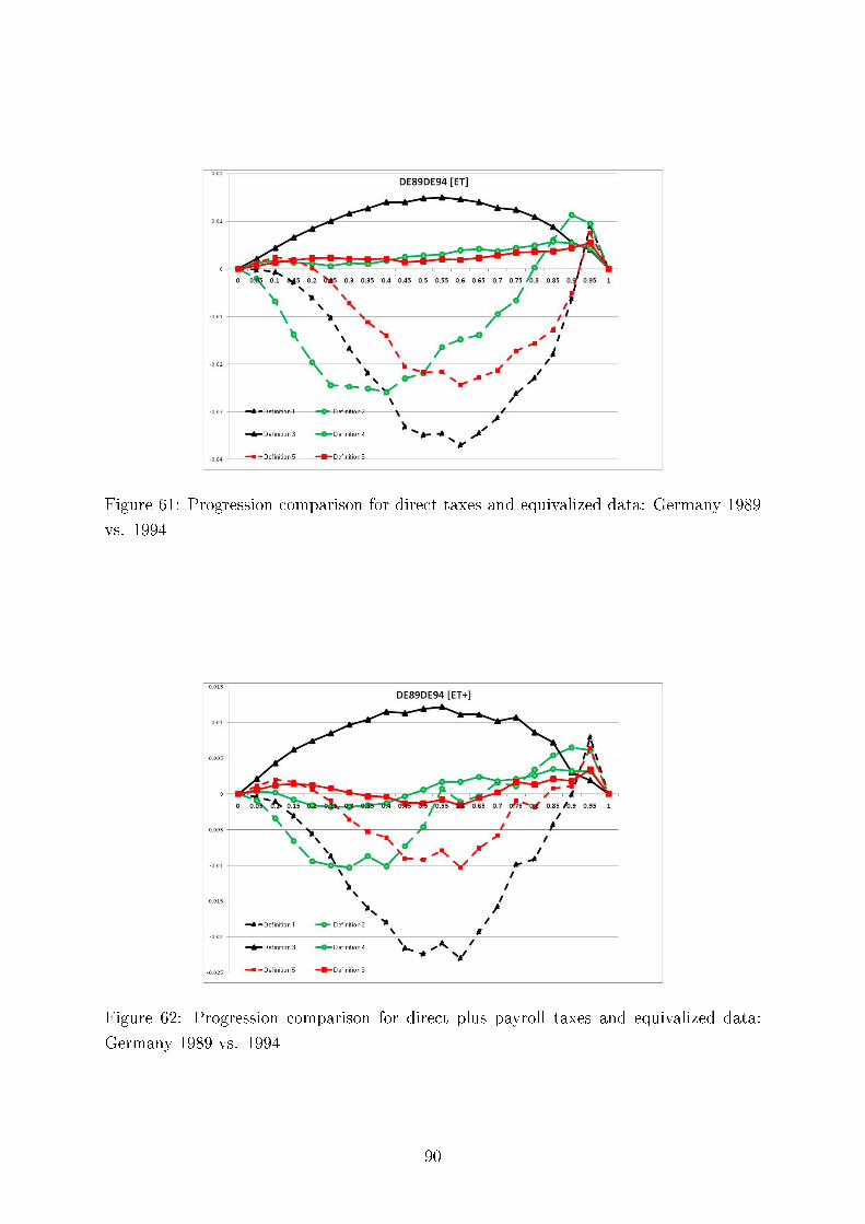
Figure 61: Progression comparison for direct taxes and equivalized data: Germany 1989

vs. 1994

Figure 62: Progression comparison for direct plus payroll taxes and equivalized data:

Germany 1989 vs. 1994

90

Figure 63: Progression comparison for direct taxes and household data: Germany 1994

vs. 2000

Figure 64: Progression comparison for direct plus payroll taxes and household data:

Germany 1994 vs. 2000

91

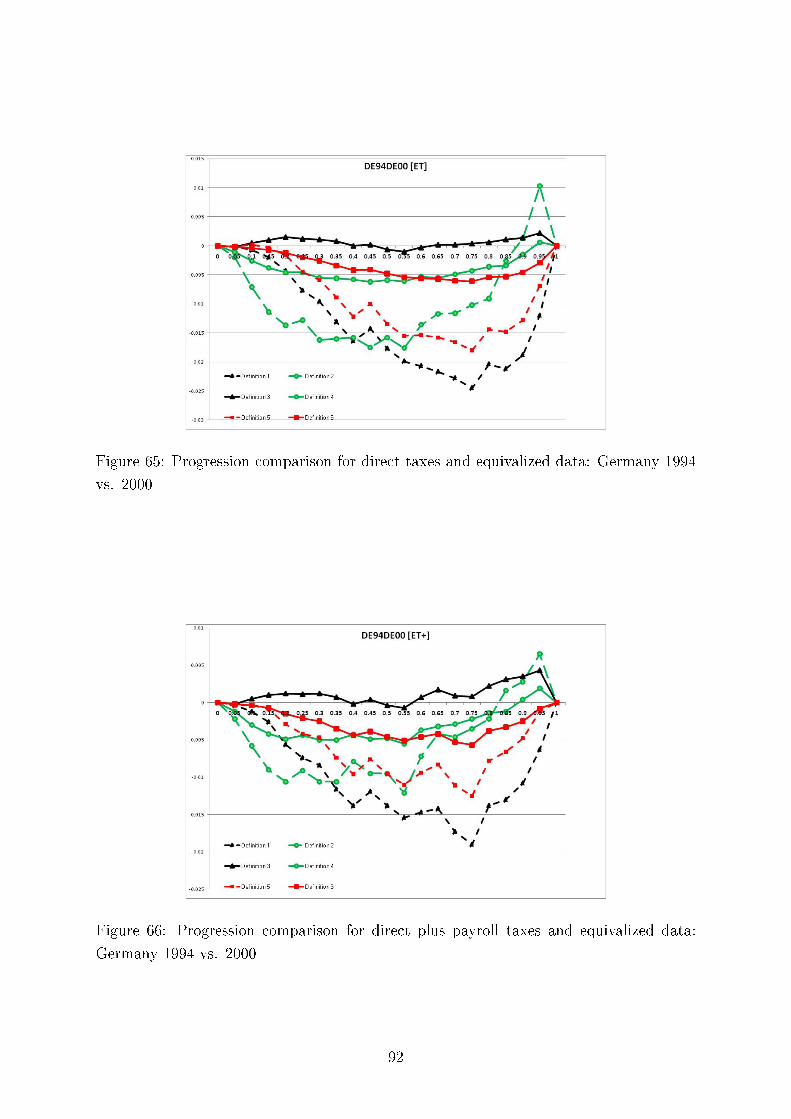
Figure 65: Progression comparison for direct taxes and equivalized data: Germany 1994

vs. 2000

Figure 66: Progression comparison for direct plus payroll taxes and equivalized data:

Germany 1994 vs. 2000

92

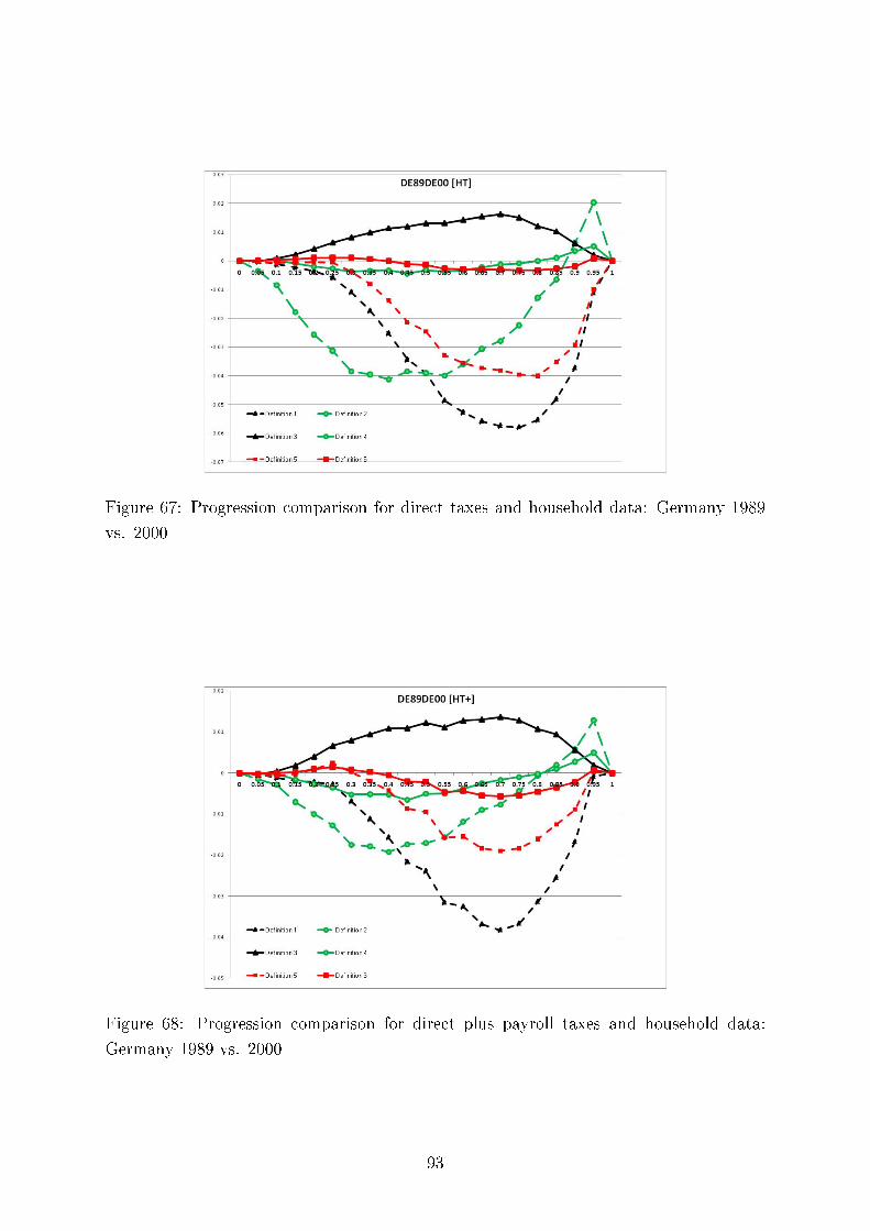
Figure 67: Progression comparison for direct taxes and household data: Germany 1989

vs. 2000

Figure 68: Progression comparison for direct plus payroll taxes and household data:

Germany 1989 vs. 2000

93

Figure 69: Progression comparison for direct taxes and equivalized data: Germany 1989

vs. 2000

Figure 70: Progression comparison for direct plus payroll taxes and equivalized data:

Germany 1989 vs. 2000

94

Figure 71: Progression comparison for direct plus payroll taxes and scale parameters 0.25

and 0.50: United States 1991

Figure 72: Progression comparison for direct plus payroll taxes and scale parameters 0.25

and 0.50: United States 1994

95

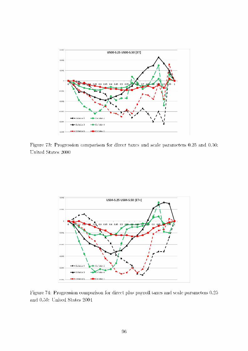
Figure 73: Progression comparison for direct taxes and scale parameters 0.25 and 0.50:

United States 2000

Figure 74: Progression comparison for direct plus payroll taxes and scale parameters 0.25

and 0.50: United States 2004

96

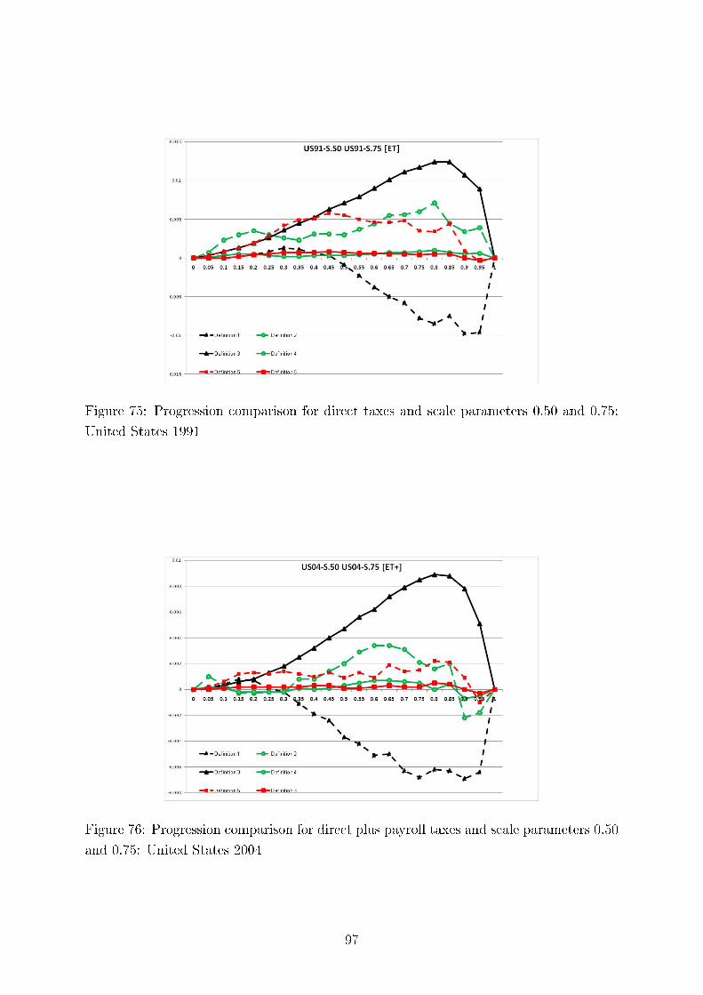
Figure 75: Progression comparison for direct taxes and scale parameters 0.50 and 0.75:

United States 1991

Figure 76: Progression comparison for direct plus payroll taxes and scale parameters 0.50

and 0.75: United States 2004

97

Figure 77: Progression comparison for direct plus payroll taxes and scale parameters 0.25

and 0.75: United States 1994

Figure 78: Progression comparison for direct plus payroll taxes and scale parameters 0.25

and 0.75: United States 2000

98

Figure 79: Progression comparison for direct plus payroll taxes and scale parameters 0.25

and 0.50: United Kingdom 1991

Figure 80: Progression comparison for direct taxes and scale parameters 0.25 and 0.50:

United Kingdom 1999

99

Figure 81: Progression comparison for direct taxes and scale parameters 0.25 and 0.50:

United Kingdom 2004

Figure 82: Progression comparison for direct taxes and scale parameters 0.50 and 0.75:

United Kingdom 1991

100

Figure 83: Progression comparison for direct taxes and scale parameters 0.50 and 0.75:

United Kingdom 1995

Figure 84: Progression comparison for direct taxes and scale parameters 0.25 and 0.75:

United Kingdom 1999

101

Figure 85: Progression comparison for direct taxes and scale parameters 0.50 and 0.75:

United Kingdom 2004

Figure 86: Progression comparison for direct plus payroll taxes and scale parameters 0.25

and 0.75: United Kingdom 1991

102

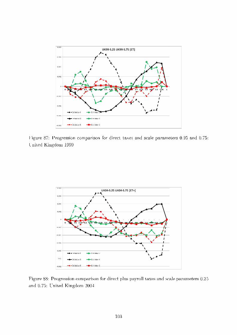
Figure 87: Progression comparison for direct taxes and scale parameters 0.25 and 0.75:

United Kingdom 1999

Figure 88: Progression comparison for direct plus payroll taxes and scale parameters 0.25

and 0.75: United Kingdom 2004

103

Figure 89: Progression comparison for direct plus payroll taxes and scale parameters 0.25

and 0.50: Germany 1989

Figure 90: Progression comparison for direct plus payroll taxes and scale parameters 0.25

and 0.50: Germany 1994

104

Figure 91: Progression comparison for direct plus payroll taxes and scale parameters 0.25

and 0.50: Germany 2000

Figure 92: Progression comparison for direct taxes and scale parameters 0.50 and 0.75:

Germany 1989

105

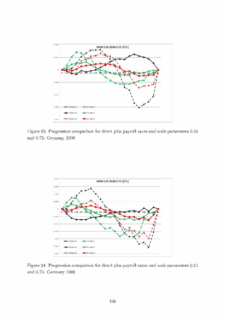
Figure 93: Progression comparison for direct plus payroll taxes and scale parameters 0.50

and 0.75: Germany 2000

Figure 94: Progression comparison for direct plus payroll taxes and scale parameters 0.25

and 0.75: Germany 1989

106

Figure 95: Progression comparison for direct taxes and scale parameters 0.25 and 0.75:

Germany 1994

Figure 96: Progression comparison for direct plus payroll taxes and scale parameters 0.25

and 0.75: Germany 2000

107