Lyapunov methods in robustness—an overview

Franco Blanchini,Dipartimento di Matematica

e Informatica,Universita di Udine,33100 Udine, Italyblanchini@uniud.it

03/June/2016

Abstract

In this survey we present some basic results and concepts concerning the robust analysisand synthesis of uncertain systems based on Lyapunov methods.

Index terms– Uncertain Systems, Lyapunov Function, Robustness.

1 Introduction

Any model of a real system presents inaccuracies. This is the reason why robustness with respectto system variations is perhaps one of the most important aspects in the analysis and control ofdynamical systems. In simple words, a system which has to guarantee certain properties, is saidrobust if satisfies the requirements not only for its nominal values but also in the presence ofperturbations. In this survey we present an overview of a specific approach to system robustnessand precisely that based on the Lyapunov theory. Although this approach is a classical one,it is still of great interest in view of the powerful tools it considers. We first introduce somegeneric concepts related to the theory of Lyapunov Functions and Control Lyapunov Functions.Then we investigate more specific topics such that the stability and stabilization via quadraticLyapunov functions. We subsequently discuss some classes of non–quadratic functions such asthe polyhedral ones. We finally briefly present some successful applications of the theory.

1.1 The concept of robustness

The term robustness is deeply known in control theory since any real system is affected byuncertainties. Uncertainties may be of different nature and they can be essentially divided inthe following categories.

• Unpredictable events.

• Unmodelled dynamics.

• Unavailable data.

Unpredictable events are typically those due to factors which perturb the systems and dependson the external environment (i.e. the air turbulence for an aircraft). Unmodeled dynamics istypical in any system modeling in which a simplification is necessary to have a reasonably simplemodel (for instance if we consider the air pressure inside a plenum in dynamic conditions weoften forget about the fact that the pressure is not in general uniform in space). Unavailabledata is a very frequent problem in practice since in many cases some quantities are known onlywhen the system operates (how much weight will be carried by a lift?).

Therefore, during the design stage, we cannot consider a single system but a family ofsystems. Formally the concept of robustness can be stated as follows.

Definition 1.1 A property P is said robust for the family F of dynamic systems if any memberof F satisfies P

The family F and the property P must be properly specified. For instance if P is “stability”and F is a family of systems with uncertain parameters ranging in a set, we have to specify ifthese parameters are constant or time–varying.

In the context of robustness the family F represents the uncertainty in the knowledge of thesystem. There are basically two categories of uncertainties. Precisely we talk about

Parametric uncertainties : when we deal with a class of models depending upon parameterswhich are unknown; in this case the typical available information is given by bounds onthese parameters:

2

Non–parametric uncertainties : when we deal with a systems in which some of the com-ponents are not modeled; the typical available information is provided in terms of theinput–output–induced norm of some operator.

In this work we mainly consider parametric uncertainties.

Example 1.1 Consider the system represented in Fig. 1 having equations

zy

m Mu

Figure 1: The elastic system

My(t) = k(z − y) + α(z − y) + u

mz(t) = k(y − z) + α(y − z)

where z and x represent the distance from the equilibrium position, M is the known mass of themain body subject to the force u and where m is the mass of another object elastically connectedto the previous. A typical situation is that in which the elastic constant k, the friction α and themass m are not known. This situation can be modeled in two ways. The first is to take theseequations as they are and impose some bound to the parameters as

k− ≤ k ≤ k+, m− ≤ m ≤ m+, α− ≤ α ≤ α+.

A different possibility is the following. Consider the new variables η = k(z − y) + α(z − y) andξ = y. Then we can write (by adopting the Laplace transform)

Ms2y(s) = u(s)− η(s),

ξ(s) = y(s)

η(s) = ∆(s)ξ(s)

where

∆(s) =ms2(αs+ k)

ms2 + αs+ k

This corresponds to the situation depicted in Fig. 2. The connected object is represented by thetransfer function ∆(s) (more in general an operator) which is unknown–but–bounded. A typicalassumption on this kind of uncertainties is that ∆(s) is stable and norm–bounded as

‖∆‖ ≤ µ

where ‖ · ‖ any appropriate norm for the transfer function. A quite commonly used norm is

‖∆‖ = supω≥0

|∆(jω)|

3

∆

P

ξ

yu

η

Figure 2: The delta configuration

(in the considered example its value is k although, in principle, the example does not fit inthe considered uncertainties since it is not stable). The main advantage of this setup is thatone can consider specification of the form ‖∆‖ ≤ µ even if the equations of the device are notknown since such kind of uncertainty specifications do not depend on the physical structure.The shortcoming is that this kind of uncertain specification are quite often a very rough andconservative approximation of the true uncertainties.

1.2 Time varying parameters

As mentioned above, the family of systems under consideration is represented by a parameterizedmodel in which the parameters are uncertain but they are known to take their values in aprescribed set. Then a fundamental distinction has to be considered.

• The parameters are unknown but constant;

• The parameters are unknown and time–varying;

Even if we consider the same bound for a parameter of a vector of parameters, assuming itconstant or time varying may lead to complete different situations. Indeed parameter variationmay have a crucial effect on stability. Consider the system

x(t) = A(w(t))x(t)

with

A(w) =

[

0 1−1 + w −a

]

|w| ≤ w,

where a > 0 is a damping parameter and w < 1 is an uncertainty bound.

For any constant w < w and a > 0, the corresponding time-invariant system is stable.However, there exists w < 1 and a (small enough) such that for suitable time-varying w(t), with|w(t)| ≤ w, the system is unstable (precisely ‖x(t)‖ diverges if x(0) 6= 0). This model is not onlyan academic example. Indeed it can be physically relized as shown in Fig. 1.2 The equation of

4

θ

this system isJθ(t) = −(g + b(t)) sin(θ(t))− a(t)θ(t)

where b(t) is the vertical acceleration of the reference frame. For small variations this equationbecomes

Jθ(t) = −(g + b(t))θ(t)− a(t)θ(t)

which is the considered type.

A further distinction is important as far as we are considering a stabilization problem. Thefact that the parameters are “unknown” may be intended in two ways.

• The parameter are unknown in the design stage but are measurable on–line.

• The parameter are unknown and not measurable on–line.

Obviously (with some exceptions) the possibility of measuring the parameter on–line is anadvantage. The compensator which modifies its parameter based on the parameter measurementare often referred to as gain–scheduling or full information. The compensator which do not havethis option, are called robust.

2 State space models

In most of the work we consider systems that, in the most general case, are governed by ordinarydifferential equations of the form

x(t) = f(x(t), w(t), u(t)) (1)

y(t) = h(x(t), w(t)) (2)

or by difference equations of the form

x(t+ 1) = f(x(t), w(t), u(t)) (3)

y(t) = h(x(t), w(t)) (4)

where x(t) ∈ IRn is the system state, w(t) ∈ IRq is an external input (non controllable and whosenature will be specified later), u(t) ∈ IRm is a control input and y(t) is the system output. Being

5

the paper mainly devoted to control problems, we introduce the expression of the most generalform of dynamic finite–dimensional regulator we are considering and precisely

xc(t) = fc(xc(t), w(t), y(t)) (5)

u(t) = hc(xc(t), w(t), y(t)) (6)

or, in the discrete–time case,

xc(t+ 1) = fc(xc(t), w(t), y(t)) (7)

u(t) = hc(xc(t), w(t), y(t)) (8)

Note that no control action has been considered in the output equation (2) and (4) and thisassures the well posedness of the feedback connection.

It is well known that the connection of the systems (1)-(2) and (5)-(6) produces a dynamicsystems of augmented dimension whose state is the compound vector

z(t) =

[

x(t)xc(t)

]

(9)

This state augmentation, intrinsic of a feedback loop, may trouble a theory which has the statespace as natural environment. This is not a trouble (as long as the dimension of xc(t) is known)because a dynamic feedback can be always regarded as the static feedback

v(t) = fc(xc(t), w(t), y(t))

u(t) = hc(xc(t), w(t), y(t))

for the augmented system

z(t) =

[

x(t)xc(t)

]

=

[

f(x(t), w(t), u(t))v(t)

]

(10)

with outputy(t) = h(x(t), w(t))

Therefore, with few exceptions, we will usually refer to static type of control systems. Obviouslythe same considerations can be done for the discrete-time version of the problem.

In some problems the equations above have to be considered along with constraints whichare imposed on both control and output, typically of the form

u(t) ∈ U (11)

andy(t) ∈ Y (12)

where U ⊂ IRm and Y ⊂ IRp are assigned “admissible” sets.

As far as the input w(t) is concerned, this signal can play several roles depending on theproblem, such as that of the reference signal, that of the noise or that of a time–varying parametervector. A typical specification for such a function is given in the form

w(t) ∈ W (13)

6

The set W will be therefore either the set of variation of the admissible reference signals or theset of possible variation of an unknown–but–bounded parameter.

An important comment concerns the compensator nature. Any compensator is assumed to bedesigned for a specific purpose. Then let us assume that the compensator has to assure a certainproperty, say property P to the closed loop system. We will use the following terminology. Thecompensator is

Gain scheduled if it is of the form (5) (6) (respectively (7) (8)) with no restrictions. Findinga control of this form which assures property P is a gain–scheduling design problem.

Robust if we assume that the compensator equations are independent on w we will name thecontroller robust and we say that P is satisfied robustly. Designing a compensator is whichindependent of w is a robust design problem.

The joint presence of a control u(t) and the signal w(t) can be also interpreted in terms ofdynamic game theory in which two individuals u, the “good guy”, and w, the “bad guy”, playagainst each other with opposite goals [6].

3 Notations

Throughout the paper we will use the following notations. Given a function Ψ(x) we define thesub-level set

N [Ψ, β] = x : Ψ(x) ≤ β.and the set

N [Ψ, α, β] = x : α ≤ Ψ(x) ≤ β.If Ψ is differentiable, we denote by

∇Ψ(x) = [∂Ψ

∂x1

∂Ψ

∂x2. . .

∂Ψ

∂xn]

its gradient. Given a matrix P we use the standard notation

P > (≥, <,≤) 0 ⇔ xTPx > (≥, <,≤) 0, ∀x 6= 0.

We say that φ : IR+ → IR+ is a κ–function if it is continuous, strictly increasing and φ(0) = 0.

4 Lyapunov derivative

In this work we will refer to systems which do not have the standard regularity property (insome cases they are not even continuous) and Lyapunov functions which are non differentiable.As a consequence this section which introduces preliminary material is quite involved. Indeedto render the exposition rigorous from a mathematical point of view we need to introduce thederivative in a generalized sense (the Dini derivative). On the other hand, the reader who isnot mathematically oriented should not be discouraged from reading the work since the fullcomprehension of this section is not strictly necessary for the comprehension of the following

7

chapters. Given a differentiable function Ψ : IRn → IR and a derivable trajectory x(t) we canalways consider the composed function Ψ(x(t)) whose derivarive is

Ψ(x(t)) = ∇Ψ(x(t))x(t)

It is well known from the elementary theory of Lyapunov that this is a preliminary step to definethe Lyapunov derivative. If the trajectory is generated by the system x(t) = f(x(t)) and at timet we have x(t) = x, then we can determine Ψ without the knowledge of the solution x(t)

Ψ(x(t))|x(t)=x = ∇Ψ(x)x = ∇Ψ(x)f(x)

which is a function of x. Unfortunately, writing Ψ in this way is not possible if either Ψ is notdifferentiable or x is not derivable.

Nevertheless, the reader can always consider the material of the section by “taking thepicture” instead of entering in the detail of the Dini derivative if this concept turns out to betoo nasty.

4.1 Solution of a system of differential equations

Consider a system of the form (possibly resulting from a feedback connection)

x(t) = f(x(t), w(t)) (14)

We will always assume that w(t) is a piecewise continuous function of time. Unfortunately, wecannot rely on continuity assumptions of the function f , since we will sometimes refer to systemswith discontinuous controllers. This will cause some mathematical difficulties.

Definition 4.1 Given a function x : IR+ → IRn, which is componentwise absolutely continuousin any compact interval we say that x is a solution if it satisfies (14) for almost all t ≥ 0.

The above definition is quite general, but it is necessary to deal with problems in which thesolution x(t) is not derivable. It is known that under more stronger assumptions, such ascontinuity of both w and f , the solution is differentiable everywhere in the regular sense. Inmost of the paper (but with several exception) we will refer to differential functions admittingregular (i.e. differentiable everywhere) solutions. As far as the existence of global solution (i.e.defined on all the positive axis IR+) we will not enter in this question since we always assumethat the system (14) will be globally solvable. In particular, we will not consider equations withfinite escape time.

4.2 The upper right Dini derivative

Let us now consider a function Ψ : IRn → IR defined and locally Lipschitz on the state space.As long as we are interested in the behavior of this function in terms of its monotonicity alongthe system trajectories we need to exploit the concept of Lyapunov derivative along the systemtrajectory. For any solution x(t), we can consider the composed function

ψ(t).= Ψ(x(t))

8

This new function ψ(t) is not usually differentiable. However, the composition of a locallyLipschitz function Ψ and an absolutely continuous function is also absolutely continuous, andthus it is differentiable almost everywhere. Therefore we need to introduce the upper right Diniderivative defined as

D+ψ(t).= lim sup

h→0+

ψ(t+ h)− ψ(t)

h(15)

As long as the function ψ(t) is derivable in the regular sense we have just that

D+ψ(t) = ψ(t).

There are four Dini derivatives which are said upper or lower if we consider limsup or liminf andthey are said right or left if we consider the right or left limit in the quotient ratio. These aredenoted as D+, D+, D

− and D−. We limit our attention only to D+. If an absolutely continuousfunction ψ(t) defined on and interval [t1, t2], has the right Dini derivative D+ψ(t) nonpositivealmost everywhere, than it is non–increasing on such interval as in the case of differentiablefunctions. The assumption of absolute continuity is fundamental, because there exist examplesof continuous functions with zero derivative almost everywhere which are indeed increasing.

4.3 Derivative along the solution of a differential equation

Let us consider again a locally Lipschitz function Ψ : IRn → IR and a solution x(t) of thedifferential equation (14). A key point of the theory of Lyapunov is that as long as we wishto consider the derivative of the composed function ψ(t) = Ψ(x(t)) we do not need to knowx(·) as a function of time but just the current value x(t) and w(t). Let us introduce the upperdirectional derivative of Ψ with respect to (14) as

D+Ψ(x,w).= lim sup

h→0+

Ψ(x+ hf(x,w))−Ψ(x)

h(16)

The next fundamental property holds (see [51], Appendix. 1, Th. 4.3)

Theorem 4.1 If the absolutely continuous function x(t) is a solution of the differential equation(14), Ψ : IRn → IR is a locally Lipschitz function and if we define ψ(t) = Ψ(x(t)), then we have

D+ψ(t) = D+Ψ(x(t), w(t)) (17)

almost everywhere in t.

The next theorem will be also useful in the sequel.

Theorem 4.2 If the absolutely continuous function x(t) is a solution of the differential equation(14), Ψ : IRn → IR a locally Lipschitz function and we define ψ(t) = Ψ(x(t)) then we have forall 0 ≤ t1 ≤ t2

ψ(t2)− ψ(t1) =

∫ t2

t1

D+ψ(σ) dσ =

∫ t2

t1

D+Ψ(x(σ), w(σ)) dσ (18)

9

4.4 Special cases of directional derivatives

There are special but important cases in which the Lyapunov derivative admits an explicitexpression, since the directional derivative can be written in a simple way. The most famousand popular case is that in which the function Ψ is continuously differentiable.

Proposition 1 Assume that Ψ is continuously differentiable on IRn, then

D+Ψ(x,w) = ∇Ψ(x)f(x,w), (19)

(where we remind that ∇Ψ(x) = [∂Ψ(x)/∂x1 ∂Ψ(x)/∂x2 . . . ∂Ψ(x)/∂xn])

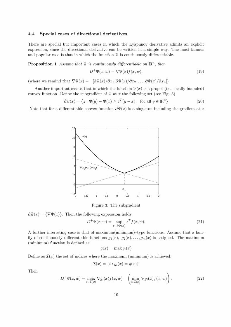
Another important case is that in which the function Ψ(x) is a proper (i.e. locally bounded)convex function. Define the subgradient of Ψ at x the following set (see Fig. 3)

∂Ψ(x) = z : Ψ(y)−Ψ(x) ≥ zT (y − x), for all y ∈ IRn (20)

Note that for a differentiable convex function ∂Ψ(x) is a singleton including the gradient at x

−2 −1.5 −1 −0.5 0 0.5 1 1.5 2−2

0

2

4

6

8

10

12

x 1

Ψ(x)

Ψ(x1)+zT(x−x

1)

Figure 3: The subgradient

∂Ψ(x) = ∇Ψ(x). Then the following expression holds.

D+Ψ(x,w) = supz∈∂Ψ(x)

zT f(x,w). (21)

A further interesting case is that of maximum(minimum)–type functions. Assume that a fam-ily of continuously differentiable functions g1(x), g2(x), . . . , gm(x) is assigned. The maximum(minimum) function is defined as

g(x) = maxigi(x)

Define as I(x) the set of indices where the maximum (minimum) is achieved:

I(x) = i : gi(x) = g(x)Then

D+Ψ(x,w) = maxi∈I(x)

∇gi(x)f(x,w)(

mini∈I(x)

∇gi(x)f(x,w))

. (22)

10

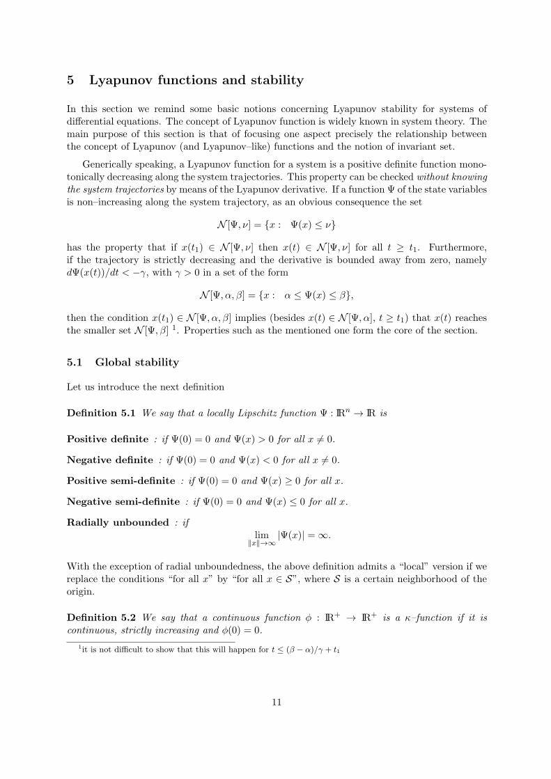
5 Lyapunov functions and stability

In this section we remind some basic notions concerning Lyapunov stability for systems ofdifferential equations. The concept of Lyapunov function is widely known in system theory. Themain purpose of this section is that of focusing one aspect precisely the relationship betweenthe concept of Lyapunov (and Lyapunov–like) functions and the notion of invariant set.

Generically speaking, a Lyapunov function for a system is a positive definite function mono-tonically decreasing along the system trajectories. This property can be checked without knowingthe system trajectories by means of the Lyapunov derivative. If a function Ψ of the state variablesis non–increasing along the system trajectory, as an obvious consequence the set

N [Ψ, ν] = x : Ψ(x) ≤ ν

has the property that if x(t1) ∈ N [Ψ, ν] then x(t) ∈ N [Ψ, ν] for all t ≥ t1. Furthermore,if the trajectory is strictly decreasing and the derivative is bounded away from zero, namelydΨ(x(t))/dt < −γ, with γ > 0 in a set of the form

N [Ψ, α, β] = x : α ≤ Ψ(x) ≤ β,

then the condition x(t1) ∈ N [Ψ, α, β] implies (besides x(t) ∈ N [Ψ, α], t ≥ t1) that x(t) reachesthe smaller set N [Ψ, β] 1. Properties such as the mentioned one form the core of the section.

5.1 Global stability

Let us introduce the next definition

Definition 5.1 We say that a locally Lipschitz function Ψ : IRn → IR is

Positive definite : if Ψ(0) = 0 and Ψ(x) > 0 for all x 6= 0.

Negative definite : if Ψ(0) = 0 and Ψ(x) < 0 for all x 6= 0.

Positive semi-definite : if Ψ(0) = 0 and Ψ(x) ≥ 0 for all x.

Negative semi-definite : if Ψ(0) = 0 and Ψ(x) ≤ 0 for all x.

Radially unbounded : iflim

‖x‖→∞|Ψ(x)| = ∞.

With the exception of radial unboundedness, the above definition admits a “local” version if wereplace the conditions “for all x” by “for all x ∈ S”, where S is a certain neighborhood of theorigin.

Definition 5.2 We say that a continuous function φ : IR+ → IR+ is a κ–function if it iscontinuous, strictly increasing and φ(0) = 0.

1it is not difficult to show that this will happen for t ≤ (β − α)/γ + t1

11

Consider a model of the form

x(t) = f(x(t), w(t)), w(t) ∈ W, (23)

and assume that the following condition is satisfied

f(0, w) = 0, for all w ∈ W (24)

which is well known to be equivalent to the fact that x(t) ≡ 0 is a trajectory of the system. Weassume that system (23) admits a solution for each x(0) ∈ IRn.

Definition 5.3 We say that system (23) is Globally Uniformly Asymptotically Stable if, for allfunctions w(t) ∈ W, it is

Locally Stable: for all ν > 0 there exists δ > 0 such that if ‖x(0)‖ ≤ δ then

‖x(t)‖ ≤ ν, for all t ≥ 0; (25)

Globally Actractive: for all µ > 0 and ǫ > 0 there exist T (µ, ǫ) > 0 such that if ‖x(0)‖ ≤ µthen

‖x(t)‖ ≤ ǫ, for all t ≥ T (µ, ǫ); (26)

Since we require that the properties of uniform stability and actractivity holds for all functionsw, the property above is often referred to as Robust Global Uniform Asymptotic Stability. Themeaning of the definition above is that for any neighborhood of the origin the evolution of thesystem is bounded inside it, provided that we start sufficiently close to 0, and it converges to zerouniformly in the sense that for all the initial states x(0) inside a µ–ball, the ultimate capture ofthe state inside any ǫ–ball occurs in a time that admits an upper bound not depending on w(t).

Definition 5.4 We say that a locally Lipschitz function Ψ : IRn → IR is a Global LyapunovFunction (GLF) for the system if it is positive definite, radially unbounded and there exists aκ–function φ such that

D+Ψ(x,w) ≤ −φ(‖x(t)‖) (27)

The following theorem is a well established result in system theory. Its first formulation isdue to Lyapunov [42] and several other versions have been introduced in the literature.

Theorem 5.1 Assume that the system (23) admits a Global Lyapunov function Ψ. Then it isglobally uniformly asymptotically stable.

Proof From Theorem 4.2 we have that

Ψ(x(t))−Ψ(x(0)) =

∫ t

0D+(x(σ), w(σ)) dσ ≤ −

∫ t

0φ(‖x(σ)‖) dσ (28)

Therefore Ψ(x(t)) is non–increasing. To show stability let ν > 0 be arbitrary and let ξ anypositive value such that N [Ψ, ξ] ⊆ N [‖ · ‖, ν]. Since Ψ is radially unbounded and positivedefinite, we have that such a ξ > 0 exists. Since Ψ is positive definite there exists δ > 0

12

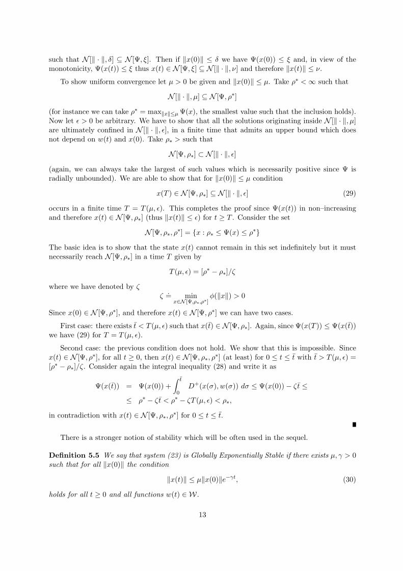
such that N [‖ · ‖, δ] ⊆ N [Ψ, ξ]. Then if ‖x(0)‖ ≤ δ we have Ψ(x(0)) ≤ ξ and, in view of themonotonicity, Ψ(x(t)) ≤ ξ thus x(t) ∈ N [Ψ, ξ] ⊆ N [‖ · ‖, ν] and therefore ‖x(t)‖ ≤ ν.

To show uniform convergence let µ > 0 be given and ‖x(0)‖ ≤ µ. Take ρ∗ <∞ such that

N [‖ · ‖, µ] ⊆ N [Ψ, ρ∗]

(for instance we can take ρ∗ = max‖x‖≤µΨ(x), the smallest value such that the inclusion holds).Now let ǫ > 0 be arbitrary. We have to show that all the solutions originating inside N [‖ · ‖, µ]are ultimately confined in N [‖ · ‖, ǫ], in a finite time that admits an upper bound which doesnot depend on w(t) and x(0). Take ρ∗ > such that

N [Ψ, ρ∗] ⊂ N [‖ · ‖, ǫ]

(again, we can always take the largest of such values which is necessarily positive since Ψ isradially unbounded). We are able to show that for ‖x(0)‖ ≤ µ condition

x(T ) ∈ N [Ψ, ρ∗] ⊆ N [‖ · ‖, ǫ] (29)

occurs in a finite time T = T (µ, ǫ). This completes the proof since Ψ(x(t)) in non–increasingand therefore x(t) ∈ N [Ψ, ρ∗] (thus ‖x(t)‖ ≤ ǫ) for t ≥ T . Consider the set

N [Ψ, ρ∗, ρ∗] = x : ρ∗ ≤ Ψ(x) ≤ ρ∗

The basic idea is to show that the state x(t) cannot remain in this set indefinitely but it mustnecessarily reach N [Ψ, ρ∗] in a time T given by

T (µ, ǫ) = [ρ∗ − ρ∗]/ζ

where we have denoted by ζζ.= min

x∈N [Ψ,ρ∗,ρ∗]φ(‖x‖) > 0

Since x(0) ∈ N [Ψ, ρ∗], and therefore x(t) ∈ N [Ψ, ρ∗] we can have two cases.

First case: there exists t < T (µ, ǫ) such that x(t) ∈ N [Ψ, ρ∗]. Again, since Ψ(x(T )) ≤ Ψ(x(t))we have (29) for T = T (µ, ǫ).

Second case: the previous condition does not hold. We show that this is impossible. Sincex(t) ∈ N [Ψ, ρ∗], for all t ≥ 0, then x(t) ∈ N [Ψ, ρ∗, ρ

∗] (at least) for 0 ≤ t ≤ t with t > T (µ, ǫ) =[ρ∗ − ρ∗]/ζ. Consider again the integral inequality (28) and write it as

Ψ(x(t)) = Ψ(x(0)) +

∫ t

0D+(x(σ), w(σ)) dσ ≤ Ψ(x(0))− ζt ≤

≤ ρ∗ − ζt < ρ∗ − ζT (µ, ǫ) < ρ∗,

in contradiction with x(t) ∈ N [Ψ, ρ∗, ρ∗] for 0 ≤ t ≤ t.

There is a stronger notion of stability which will be often used in the sequel.

Definition 5.5 We say that system (23) is Globally Exponentially Stable if there exists µ, γ > 0such that for all ‖x(0)‖ the condition

‖x(t)‖ ≤ µ‖x(0)‖e−γt, (30)

holds for all t ≥ 0 and all functions w(t) ∈ W.

13

The factor γ in the definition above will be named the convergence speed while factor µ will benamed the transient estimate. Robust exponential stability can be assured by the existence of aLyapunov function whose decreasing rate along the system trajectories is expressed in terms ofthe magnitude of the function. Let us assume that the positive definite function Ψ(x) is upperand lower polynomially bounded as

α‖x‖p ≤ Ψ(x) ≤ β‖x‖p, for all x ∈ IRn, (31)

for some positive reals α and β and some positive integer p. We have the following

Theorem 5.2 Assume that the system (23) admits a positive definite locally Lipschitz functionΨ, which has polynomial grows as in (31) and

D+Ψ(x,w) ≤ −γΨ(x) (32)

for some positive γ. Then it is Globally Exponentially Stable.

Proof Consider the integral inequality (18) and write it as

Ψ(x(t+ T )) ≤ Ψ(x(t)) +

∫ t+T

tD+Ψ(x(σ), w(σ))dσ

≤ Ψ(x(t))− γ

∫ t+T

tΨ(x(σ))dσ ≤ Ψ(x(t))− TγΨ(x(t+ T ))

where the last inequality follows by the fact that Ψ(x(t)) is non–increasing. This implies

Ψ(x(t+ T )) ≤ 1

1 + TγΨ(x(t))

Therefore for all k

Ψ(x(kT )) ≤[

1

1 + Tγ

]k

Ψ(x(0))

Let now t > 0 be arbitrary and T = t/k, with k integer. We get

Ψ(x(t)) ≤[

1

1 + γt/k

]− kγt

−γt

Ψ(x(0)) =

[1 + γt/k]kγt

−γt

Ψ(x(0))

The number inside the graph brackets converges to e as k → ∞ and since the inequality holdsfor any k, we have that

Ψ(x(t)) ≤ e−γtΨ(x(0))

Now we use condition (31) that, after simple mathematics, yields

‖x(t)‖ ≤ p

√

β

αe− γ

pt ‖x(0)‖

which implies exponential convergence with convergence speed γ/p and transient estimate p

√βα.

The previous theorem admits a trivial proof if we assume that Ψ(x(t)) is derivable in theregular sense. Indeed the inequality (32) would become the differential inequality Ψ(x(t)) ≤−γΨ(x), that implies Ψ(x(t)) ≤ e−γtΨ(x(0)). It is obvious that exponential stability impliesrobust global asymptotic stability (the proof is very easy and not reported).

14

5.2 Local stability and ultimate boundedness

Global stability can be somewhat a too ambitious requirement in practical control theory, basi-cally for the next two reasons.

• requiring convergence from arbitrary initial conditions can be too restrictive;

• in practice persistent disturbances can prevent the system from approaching the origin.

For this reason it is very useful to introduce the notion of local stability and uniform ultimateboundedness. Let us denote by S a neighborhood of the origin.

Definition 5.6 Let S be a neighborhood of the origin. We say that system (23) is UniformlyLocally Asymptotically Stable with basin of attraction S if the next two conditions hold for allfunctions w(t) ∈ W.

Local Stability : For all µ > 0 there exists δ > 0 such that ‖x(0)‖ ≤ δ implies ‖x(t)‖ ≤ µ forall t ≥ 0.

Local Uniform Convergence For all ǫ > 0 there exists T (ǫ) > 0 such that if x(0) ∈ S, then‖x(t)‖ ≤ ǫ, for all t ≥ T (ǫ);

Definition 5.7 Let S be a neighborhood of the origin. We say that system (23) is UniformlyUltimately Bounded in S if for all µ > 0 there exists T (µ) > 0 such that for ‖x(0)‖ ≤ µ

x(t) ∈ S

for all t ≥ T (µ) and all functions w(t) ∈ W.

To assure the conditions of the previous definitions we introduce the following concepts ofLyapunov functions inside and outside S.

Definition 5.8 Let S be a neighborhood of the origin. We say that the locally Lipschitz positivedefinite function is a Lyapunov function inside S if there exists ν > 0 such that

S ⊆ N [Ψ, ν]

and for all x ∈ N [Ψ, ν] the inequality

D+Ψ(x,w) ≤ −φ(‖x(t)‖)

holds for some κ–function φ.

Definition 5.9 Let S be a neighborhood of the origin. We say that the locally Lipschitz positivedefinite function is a Lyapunov function outside S if there exists ν > 0 such that

N [Ψ, ν] ⊆ S

and for all x 6∈ N [Ψ, ν] the inequality

D+Ψ(x,w) ≤ −φ(‖x(t)‖)

holds for some κ–function φ.

15

The next two theorems hold.

Theorem 5.3 Assume that the system (23) satisfying condition (24) admits a Lyapunov func-tion Ψ inside S. Then it is Locally Stable with basin of attraction S.

Theorem 5.4 Assume that the system (23) admits a Lyapunov function Ψ outside S. Then itis uniformly ultimately bounded in S.

It is intuitive that there are as many possible stability definitions as the possible numbers ofpermutation of the requirements (Global–Local–Uniform–Exponential–Robust an so on ...). Forinstance we can define exponential local stability if we require the condition (30) to be satisfiedonly for x(0) ∈ S. We can define the exponential ultimate boundedness in the set S by requiringthat N [‖ · ‖, ν] ⊂ S and ‖x(t)‖ ≤ maxµe−γt‖x(0)‖, ν. The problem is well known and in theliterature classifications of stability concepts have been proposed (see [51] section VI). Clearlyfurther investigation in this sense is beyond the scope of this paper.

6 Control Lyapunov function

In the previous section we have presented the basic results of the Lyapunov theory for a dy-namical system with an external input. We now extend these concepts to systems of the form(5) and (6) with a control input. Essentially, we define Control Lyapunov Function a positivedefinite (locally Lipschitz) function which becomes a Lyapunov functions whenever a propercontrol action is applied.

As we have observed, any dynamic finite–dimensional feedback controller can be viewed as astatic output feedback for a properly augmented system. Therefore, in this section we considera system of the form

x(t) = f(x(t), w(t), u(t))y(t) = h(x(t), w(t))

(33)

associated with a static feedback. To introduce the main definition we have to refer to a class Cof controllers. The main classes considered here are

Output feedback : if u(t) = Φ(y(t));

State feedback : if u(t) = Φ(x(t));

Output feedback with feedforward : if u(t) = Φ(y(t), w(t));

State feedback with feedforward : if u(t) = Φ(x(t), w(t)) (full information);

Definition 6.1 Given a class of controllers C and a locally Lipschitz positive definite function Ψ(and possibly a set P) we say that Ψ is a global control Lyapunov function (a Lyapunov functionoutside P or a Lyapunov function inside P) if there exists a controller in C such that:

• for each initial condition x(0) there exists a solution x(t), for any admissible w(t), andeach of such solutions is defined for all t ≥ 0;

16

• the function Ψ is a global Lyapunov function (a Lyapunov function outside P or a Lya-punov function inside P) for the closed–loop system.

An important generalization of the previous definition concerns the case of control withconstraints (11)

u(t) ∈ U .In this case we say that Ψ is a global control Lyapunov function (a Lyapunov function outsideP or a Lyapunov function inside P) if there exists a controller (in a specified class C) such that,beside the conditions in Definition 6.1, satisfies the constraints. Note also that the problem withstate constraints can be easily addressed. If we assume that

x(t) ∈ X

is a hard constraint to be satisfied, we can immediately argue that as long as N [Ψ, µ] ⊆ X ,for some µ, and Ψ is a control Lyapunov function (either global, inside or outside P), thenthe constraints can be satisfied satisfied by means of a proper control action as long as x(0) ∈N [Ψ, µ].

6.1 Associating a feedback control with a Control Lyapunov Function

According to the previous considerations we now take into account a domain of the form

N [Ψ, α, β] = x : α ≤ Ψ(x) ≤ β (34)

By possibly assuming α = 0 or β = +∞, we may include all the “meaningful” cases of Lyapunovfunction inside a set, outside a set or global. In this section we will basically consider the statefeedback and the full information feedback cases. The output feedback case will be brieflydiscussed at the end. Assume that a locally Lipschitz function Ψ is given and consider the nextinequality

D+Ψ[x, u, w].= lim sup

h→0+

Ψ(x+ hf(x, u, w))−Ψ(x)

h≤ −φ(‖x‖). (35)

Consider the next two conditions:

• For all x ∈ N [Ψ, α, β], there exists u such that (35) is satisfied for all w ∈ W;

• For all x ∈ N [Ψ, α, β], and w ∈ W there exists u such that 35 is satisfied;

These conditions are clearly necessary for Ψ to be a control Lyapunov function with state orfull information feedback, because, by definition, they are satisfied by assuming u = Φ(x) andu = Φ(x,w) respectively. A fundamental question is then the following: assume that thesecondition holds, how can we define the feedback function Φ? The problem can be thought asfollows. Let us first analyze the state feedback case. Consider the set

Ω(x) = u : (35) is satisfied for all w ∈ W

Then the question becomes whether does there exist a state feedback control function u = Φ(x)such that

Φ(x) ∈ Ω(x).

17

This question appears a philosophic one because as long as the set Ω(x) is non–empty for allx, then we can always associate with x a point u ∈ Ω(x), and “define” such a function Φ.The matter is different if one requires to the function a certain regularity such as that of beingcontinuous. This fact is important (at least from a mathematical point of view because theresulting closed–loop system must be solvable). A positive answer to this problem can be givenfor control–affine systems namely systems of the form

x(t) = a(x(t), w(t)) + b(x(t), w(t))u(t) (36)

with a and b continuous terms and with a(0, w) = 0 for all w ∈ W. Assume that continuouslydifferentiable positive definite function Ψ is given and that (35) is satisfied for all x. From thedifferentiability of Ψ we have that (35) can be written as follows

∇Ψ(x)[a(x,w) + b(x,w)u] ≤ −φ(‖x‖),

Then the set Ω(x) turns out to be

Ω(x) = u : ∇Ψ(x)b(x,w)u ≤ −∇Ψ(x)a(x,w)− φ(‖x‖), for all w ∈ W (37)

This nonempty set is convex for each x, being the intersection of hyperplanes, and together withthe continuity of a and b and the continuity of ∇Ψ(x), this property is sufficient to state thenext theorem.

Theorem 6.1 Assume that the set Ω(x) as in (37) is nonempty. Then there always exists afunction Φ : IRn → IRm continuous everywhere, possibly with the exception of the origin, suchthat

Φ(x) ∈ Ω(x) (38)

Proof See [25]

The previous theorem considers the fundamental concept of selection of a set–valued map.A set–valued map f from X to Y is a multivalued function which associates to any element xof X a subset Y of Y. A selection is a single–valued function which maps x one of the elementin Y = f(x). In our case, Ω(x) is the set–valued map of all feasible control values which assurea certain decreasing rate to the Lyapunov derivative.

In the case of full–information control, the appropriate set–valued map must be defined inthe state–disturbance product space:

Ω(x,w) = u : ∇Ψ(x)b(x,w)u ≤ −∇Ψ(x)a(x,w)− φ(‖x‖) (39)

If this set is not empty for all x and w then we may seek for a function

Φ(x,w) ∈ Ω(x,w) (40)

which is a stabilizing full–information control. In view of the convexity of the set Ω(x,w) andthe continuity, it can be shown that a continuous selection always exists, namely, that Theorem6.1 can be stated by replacing (38) by (40).

The next question is: how can we determine this function in an analytic form? To this aim,let us think first to the full information case. Let us also consider, for the moment being that the

18

region of interest is of the form N [Ψ, ǫ, κ] with k finite and ǫ small. Assume that there exists acontinuous function Ψ(x,w) which satisfies (40). Then consider the next minimum effort control[48]

ΦME(x,w) = arg minu∈Ω(x,w)

‖u‖2 (41)

(‖ · ‖2 is the euclidean norm). Such a control function always exists and it has the obviousproperty that

‖ΦME(x,w)‖ ≤ ‖Φ(x,w)‖for any admissible controller Φ(x,w), therefore it is bounded in N [Ψ, ǫ, κ]. The minimum effortcontrol admits an analytic expression which can be easily derived as follows. For fixed x and wΩ(x,w) is defined by a linear inequality for u

∇Ψ(x)b(x,w)u ≤ −∇Ψ(x)a(x,w)− φ(‖x‖) .= −c(x,w) (42)

The vector u of minimum norm which satisfies (42) can be determined analytically as follows

ΦME(x,w) =

− b(x,w)T∇Ψ(x)T

‖∇Ψ(x)b(x,w)‖2 c(x,w), if c(x,w) > 0

0, if c(x,w) ≤ 0(43)

The singularity due to the condition ∇Ψ(x)b(x,w) = 0, for some x and w is not a problem sincethis automatically implies that c(x,w) ≤ φ(‖x‖) < 0 (this is basically the reasons of workinginside the set N [Φ, ǫ, κ] with small but positive ǫ, so excluding x = 0). This expression admitsan immediate extension to the state feedback case, if we assume that the term b does not dependon w and precisely

x(t) = a(x(t), w(t)) + b(x(t))u(t)

in this case the condition becomes

∇Ψ(x)b(x)u ≤ −∇Ψ(x)a(x,w)− φ(‖x‖) .= −c(x,w) (44)

which has to be satisfied for all w by an appropriate choice of u. Define now the value

c(x) = maxw∈W

c(x,w)

which is a continuous function of x 2. The condition to be considered is then

∇Ψ(x)b(x)u ≤ −c(x) (45)

which yields the following expression for the control:

ΦME(x) =

− b(x)T∇Ψ(x)T

‖∇Ψ(x)b(x)‖2 c(x), if c(x) > 0

0, if c(x) ≤ 0(46)

The minimum effort control (46) belongs to the class of gradient–based controllers of the form

u(t) = −γ(x)b(x)T∇Ψ(x)T (47)

This type of controllers is well known and includes other types of control functions. For instanceif the control effort is not of concern, one can just consider (47) with γ(x) > 0 “sufficiently largefunction” [3]

2c(x,w) is referred to as Marginal Function see [24] for further details

19

It can be shown that as long as (46) is a suitable controller, any function having the property

γ(x) ≥ max

c(x)

‖∇Ψ(x)b(x)‖2 , 0

is also a suitable controller. This fact reveals an important property of the proposed control andprecisely

• If Ψ is a control Lyapunov function, then the controllers of the form γ(x)∇Ψ(x)b(x) haveinfinite positive gain margin in the sense that if −γ(x)b(x)T∇Ψ(x)T is a stabilizing control,then −γ′(x)b(x)T∇Ψ(x)T is also stabilizing for all γ′(x) such that γ′(x) ≥ γ(x).

The problem becomes more involved if one admits that also the term b depends on theuncertain parameters. In this case finding a state feedback controller is related to the followingmin–max problem

minu∈U

maxw∈W

∇Ψ(x)[a(x,w) + b(x,w)u] ≤ −φ(‖x‖), (48)

where, for the sake of generality, we assumed u ∈ U . If this condition is pointwise–satisfied,then there exists a robustly stabilizing feedback control. However, determining the minimizerfunction u = Φ(x) can be very hard.

An important fact worth mentioning is the relation between the above min–max problem anthe corresponding full information problem

maxw∈W

minu∈U

∇Ψ(x)[a(x,w) + b(x,w)u] ≤ −φ(‖x‖), (49)

in which the “min” and the “max” are reversed. If condition (49) is satisfied, then there exists afull information control. In fact condition (48) always implies (49). There are important classesof systems for which the two conditions are equivalent. For instance, in the case in which b doesdepend on x only, then the two problems are equivalent. This means that the existence of afull–information stabilizing controller implies the existence of a pure state feedback controller[45]. A further class of control affine uncertain systems for which the same property holds is theso called convex processes [13]

There are other forms of controllers which can be associated with a control Lyapunov func-tion. In particular an interesting class, strongly related to the minimum effort control is thelimited–effort control. Assume that the control is constrained as

‖u(t)‖ ≤ 1. (50)

Assuming the magnitude equal to 1 is not a restriction since the actual magnitude or weightingfactors can be discharged on b(x). Here essentially two norms are worth of consideration andprecisely the 2–norm ‖u‖2 =

2√uTu and the ∞–norm ‖u‖∞ = maxj |uj |. We consider the case

of local stability and we assume that a control Lyapunov function inside N [Ψ, κ] exists whichstabilizes with a control which does not violate the constraint (50).

A reasonable approach is that of considering the control which minimizes the Lyapunovderivative while preserving this bound. The problem to be solved is

min‖u‖≤1

∇Ψ(x)[a(x,w) + b(x)u]

20

For instance if we consider the two norm, this control is

u =

− b(x)T∇Ψ(x)T

‖b(x)T∇Ψ(x)T ‖if ∇Ψ(x)b(x) 6= 0,

0 if ∇Ψ(x)b(x) = 0(51)

in the case of infinity norm we have

u = −sgn[b(x)T∇Ψ(x)T ] (52)

where the sgn[v] v ∈ IRn is the component–wise sign function, (its ith component is such that(sgn[v])i = sgn[vi]). Both the controls (51) and (52) are discontinuous, but can be approximatedby the continuous controllers:

u = − b(x)T∇Ψ(x)T

‖b(x)T∇Ψ(x)T ‖+ δ

for δ sufficiently small andu = −sat[κb(x)T∇Ψ(x)T ]

for κ sufficiently large, respectively, (sat is the vector saturation function).

The literature about control Lyapunov functions is huge. This concept is of fundamentalimportance in the control of nonlinear uncertain systems. For further details, the reader isreferred to specialized work such as [24] and [34].

6.2 Output feedback case

As far as the output feedback case is concerned, the problem of determining a control to associatewith a Control Lyapunov Function is much harder. We will briefly consider the problem toexplain the reasons of these difficulties. Consider the system

x(t) = f(x(t), w(t), u(t))

y(t) = h(x(t), w(t))

and a candidate Control Lyapunov function Ψ defined on IRn. Consider a static output feedbackof the form

u(t) = Φ(y(t))

Since only output information are available, the control value u that renders the Lyapunovderivative negative must assure this property for a given output value y for all possible valuesof x and w that produce that output. Let Y be the domain of g

y = g(x,w), x ∈ IRn, w ∈ W

Given y ∈ Y define the preimage set as

g−1(y) = (x,w), x ∈ IRn, w ∈ W : y = g(x,w)

Then a condition for Ψ to be a control Lyapunov function under output feedback is then thefollowing. Consider the following set

Ω(y) = u : D+(x,w, u) ≤ −Φ(‖x‖), for all (x,w) ∈ g−1(y)

21

A necessary and sufficient condition for Φ(y) to be a proper control function is that

Φ(y) ∈ Ω(y), for all y ∈ Y (53)

This theoretical condition is simple to state, but useless in most cases, since the set g−1(y)can be hard (not to say impossible) to determine. It is not hard to find a similar theoreticalconditions for a control of the form Φ(y, w) which are again hard to apply.

So far we have considered the problem of associating a control to a Control Lyapunov Func-tion. Obviously, a major problem is how to find the function. The are lucky cases in which thefunction can be determined, but it is well known that in general, the problem is very difficultespecially in the output feedback case. Special classes of systems for which the problem is solv-able will be considered later. The reader is referred to specialized literature for further details[24] [34].

6.3 Fake Control Lyapunov functions

In this section we sketch a simple concept which is related with notions in other fields suchas the greedy or myopic strategy in Dynamic optimization. Let us introduce a very heuristicapproach to control a system. Given a plant

x(t) = f(x(t), u(t))

(we do not introduce uncertainties for brevity) and a positive definite functions ω(x), let us justadopt the following strategy that in some sense can be heuristically justified. Let us just considerthe controller (possibly among those of a certain class) that in some sense renders maximumthe decreasing rate of Ψ(x(t)), regardless of the fact that the basic condition (35) is satisfied.Assuming a constraint of the form u(t) ∈ U and assuming, for the sake of simplicity, ω to be adifferentiable function, this reduces to

u = Φ(x) = argminu∈U

∇ω(x)f(x, u)

If we assume that an integral cost of the form∫ ∞

0ω(x(t))dt

is assigned, this type of strategy is known as greedy or myopic strategy. Indeed, it minimizesthe derivative at each time in order to achieve the “best” instantaneous results. It is well knownthat this strategy is far from achieving the optimum of the integral cost (with the exception ofspecial cases [44].

What we show here is that it may also produce instability. To prove this fact, we can evenconsider the simple case of a linear time–invariant system

x(t) = Ax(t) +Bu(t)

with a scalar input u and the function

ω(x) = xTPx

Consider the case in which the system (A,B,BTP ) is strictly non–minimum phase, preciselyF (s) = BTP (sI − A)−1B admits zeros with positive real parts. Now let us first consider a

22

gradient–based controller which tries to render the derivative ω(x(t)) = 2xTP (Ax + Bu) asnegative as possible. According to the previous considerations the gradient–based control is inthis case

u(t) = −γBTPx(t)

with γ a large positive. However, due to the non–minimum phase nature of the system thiscontrol can lead the system to instability. If one considers a limitation for the input such as|u| ≤ 1, the pointwise minimizing control is

u = arg min|u|≤1

2xTP (Ax+Bu) = −sgn[xTPB]

As it is known this system becomes locally unstable at the origin if, as we have assumed,A,B,BTP is strictly non–minimum phase.

Example 6.1 Consider the (open–loop stable!) linear system with

A =

[

1 −22 −3

]

B =

[

01

]

P = I

It is immediate that the gradient based controller is

u = −γBTP = −γx2

and destabilizes the systems to instability for γ ≥ 1. The discontinuous control

u = −sgn[x2]

clearly produces similar destabilizing effects as well as its “approximation”

u = −sat[γx2].

7 Discrete–time systems

We have presented the main concepts of this section in the context of continuous–time systems.However the same concepts hold in the case of discrete–time systems although there are severaltechnical differences.

Let us now consider the case of a system (possibly resulting from a feedback connection) ofthe form

x(t+ 1) = f(x(t), w(t)) (54)

where now functions x(t) and w(t) ∈ W are indeed sequences, although they will be referred to“functions” as well. Let us now consider a function Ψ : IRn → IR defined and continuous on thestate space. It is known that, as a counterpart of the Lyapunov derivative we have to considerthe Lyapunov difference. Again, for any solution x(t), we can consider the composed function

ψ(t).= Ψ(x(t))

and let us consider the increment

∆Ψ(t) = Ψ(t+ 1)−Ψ(t) = Ψ(x(t+ 1))−Ψ(x(t))

23

Then the Lyapunov difference is defined

∆Ψ(t) = Ψ(f(x(t), w(t)))−Ψ(x(t)).= ∆Ψ(x(t), w(t)) (55)

Therefore the behavior of the function Ψ along the system trajectories can be studied by con-sidering the function ∆Ψ(x,w), thought as a function of x and w.

Consider a model of the form (54) and again assume that the following condition is satisfied

f(0, w) = 0, for all w ∈ W (56)

namely, x(t) ≡ 0 is a trajectory of the system.

For this discrete–time model the same definitions of uniform asymptotic stability (Definition5.3) holds unchanged. Definition 5.4 of global Lyapunov function remains unchanged up to thefact that we replace the Lyapunov derivative with the Lyapunov difference.

Definition 7.1 We say that a locally Lipschitz function Ψ : IRn → IR is a Global LyapunovFunction (GLF) for the system if it is positive definite, radially unbounded and there exists aκ–function φ such that

∆Ψ(x,w) ≤ −φ(‖x(t)‖) (57)

The next theorem is the discrete–time counterpart of Theorem 5.1.

Theorem 7.1 Assume that the system (54) admits a Lyapunov function Ψ. Then it is globallyuniformly stable.

Also in the discrete–time case we can introduce a stronger notion namely the exponentialstability.

Definition 7.2 We say that system (23) is Globally Exponentially Robustly Stable if there existsa positive λ < 1 such that for all ‖x(0)‖ we have the condition

‖x(t)‖ ≤ µ‖x(0)‖λt (58)

for all t ≥ 0 and all sequences w(t) ∈ W.

The coefficient λ is the discrete–time convergence speed. As in the discrete–time case exponentialstability can be assured by the existence of a Lyapunov function whose decreasing rate alongthe system trajectories is expressed in terms of the magnitude of the function. Let us assumethat the positive definite function Ψ(x) is upper and lower polynomially bounded, as in (31).We have the following

Theorem 7.2 Assume that the system (54) admits a positive definite locally Lipschitz functionΨ, which has polynomial grows as in (31) and

∆Ψ(x,w) ≤ βΨ(x) (59)

for some positive β < 1. Then it is globally exponentially uniformly stable with speed of conver-gence λ = (1− β) < 1.

24

Proof It is left as an exercise to the reader.

Note that the condition (59) of the theorem may be equivalently stated as

Ψ(f(x,w)) ≤ λΨ(x)

for all x and w ∈ W.

The concept of Local Stability and Uniform Ultimate Boundedness for discrete–time systemare introduced by Definitions 5.6 and 5.7 which hold without modifications. The concepts ofLyapunov functions inside and outside S sounds now as follows.

Definition 7.3 We say that the locally Lipschitz positive definite function is a Lyapunov func-tion inside S if there exists ν > 0 such that S ⊆ N [Ψ, ν] and for all x ∈ N [Ψ, ν] the inequality

∆Ψ(x,w) ≤ −φ(‖x(t)‖)

holds for some κ–function φ and all w ∈ W.

Definition 7.4 We say that the locally Lipschitz positive definite function is a Lyapunov func-tion outside S if there exists ν > 0 such that N [Ψ, ν] ⊆ S and for all x 6∈ N [Ψ, ν] the inequality

∆Ψ(x,w) ≤ −φ(‖x(t)‖)

holds for some κ–function φ andΨ(f(x,w)) ≤ ν

for all x ∈ N [Ψ, ν] and all w ∈ W.

Note that the last condition in the previous definition has no analogous statement in Definition5.9 and its meaning is that once the set N [Ψ, ν] is reached by the state, it cannot be escaped.This condition is automatically satisfied in the continuous time. The next two theorems hold.

Theorem 7.3 Assume that the system (54) admits a positive definite locally Lipschitz functionΨ inside S. Then it is Locally Stable with basin of attraction S.

Theorem 7.4 Assume that the system (54) admits a positive definite locally Lipschitz functionΨ outside S. Then it is uniformly ultimately bounded in S.

We consider now the case of a controlled discrete–time system (7) and (8). As we haveobserved, any dynamic finite–dimensional feedback controller can be viewed as a static outputfeedback for a properly augmented system. Therefore, we consider a system of the form

x(t) = f(x(t), w(t), u(t))y(t) = h(x(t), w(t))

(60)

associated with a static feedback. Again we should refer to one of the classes of controllers spec-ified above: output feedback, state feedback output feedback with feedforward, state feedbackwith feedforward.

25

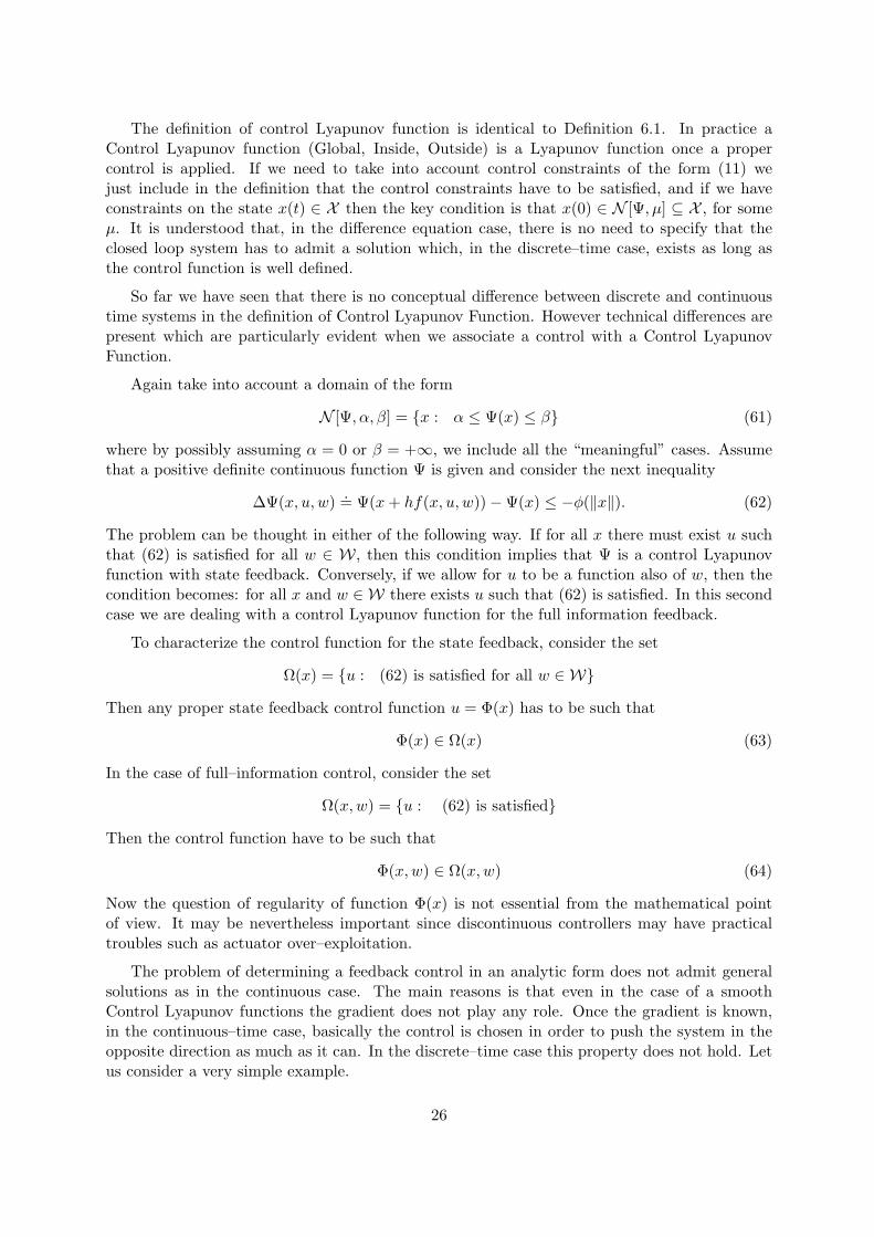
The definition of control Lyapunov function is identical to Definition 6.1. In practice aControl Lyapunov function (Global, Inside, Outside) is a Lyapunov function once a propercontrol is applied. If we need to take into account control constraints of the form (11) wejust include in the definition that the control constraints have to be satisfied, and if we haveconstraints on the state x(t) ∈ X then the key condition is that x(0) ∈ N [Ψ, µ] ⊆ X , for someµ. It is understood that, in the difference equation case, there is no need to specify that theclosed loop system has to admit a solution which, in the discrete–time case, exists as long asthe control function is well defined.

So far we have seen that there is no conceptual difference between discrete and continuoustime systems in the definition of Control Lyapunov Function. However technical differences arepresent which are particularly evident when we associate a control with a Control LyapunovFunction.

Again take into account a domain of the form

N [Ψ, α, β] = x : α ≤ Ψ(x) ≤ β (61)

where by possibly assuming α = 0 or β = +∞, we include all the “meaningful” cases. Assumethat a positive definite continuous function Ψ is given and consider the next inequality

∆Ψ(x, u, w).= Ψ(x+ hf(x, u, w))−Ψ(x) ≤ −φ(‖x‖). (62)

The problem can be thought in either of the following way. If for all x there must exist u suchthat (62) is satisfied for all w ∈ W, then this condition implies that Ψ is a control Lyapunovfunction with state feedback. Conversely, if we allow for u to be a function also of w, then thecondition becomes: for all x and w ∈ W there exists u such that (62) is satisfied. In this secondcase we are dealing with a control Lyapunov function for the full information feedback.

To characterize the control function for the state feedback, consider the set

Ω(x) = u : (62) is satisfied for all w ∈ W

Then any proper state feedback control function u = Φ(x) has to be such that

Φ(x) ∈ Ω(x) (63)

In the case of full–information control, consider the set

Ω(x,w) = u : (62) is satisfied

Then the control function have to be such that

Φ(x,w) ∈ Ω(x,w) (64)

Now the question of regularity of function Φ(x) is not essential from the mathematical pointof view. It may be nevertheless important since discontinuous controllers may have practicaltroubles such as actuator over–exploitation.

The problem of determining a feedback control in an analytic form does not admit generalsolutions as in the continuous case. The main reasons is that even in the case of a smoothControl Lyapunov functions the gradient does not play any role. Once the gradient is known,in the continuous–time case, basically the control is chosen in order to push the system in theopposite direction as much as it can. In the discrete–time case this property does not hold. Letus consider a very simple example.

26

Example 7.1 Let us seek for a state feedback for the scalar system

x(t) (x(t+ 1)) = f(x(t), w(t)) + u(t), |w| ≤ 1. (65)

Assume that |f(x(t), w(t))| ≤ ξ|x|. Consider the control Lyapunov function x2/2. The con-tinuous time problem is straight forward. Since the “gradient” is x take u pushing against forinstance u = −κx with κ large enough, in any case κ > ξ. The Lyapunov derivative is

x[f(x,w) + u] ≤ −(κ− ξ)x2

so the closed–loop system is globally asymptotically stable.

The discrete–time version of the problem is completely different. To have the Lyapunovfunction x2/2 decreasing the basic condition is:

[f(x,w) + u(x)]2 − x2 ≤ −φ(|x|), for all |w| ≤ 1

The only information we can derive is that u(x) has to be such that

u(x) ∈ Ω(x) = x : [f(x,w) + u(x)]2 ≤ x2 − φ(|x|), for all |w| ≤ 1

this condition heavily involves function f . Furthermore, it is not difficult to show that thebound |f(x(t), w(t))| ≤ ξ|x| does not assure a non–empty Ω(x) for all x (hence the systemstabilizability). For instance the system

x(t+ 1) = [a+ bw(t)]x+ u(t), |w| ≤ 1. (66)

is not stabilizable by state feedback for all values of the constant a and b. A necessary andsufficient stabilizability condition via state feedback is |b| < 1.

The previous example shows that there are no analogous controllers of that proposed foruncertain systems in [3] for continuous–time systems. By the way, one can see that the discretetime system (66) is always stabilizable by means of the full information feedback u = −f(x,w).This implies that the equivalence between state and full information feedback shown in [45] doesnot hold in the discrete–time case.

7.1 Literature Review

Needless to say, the literature on the Lyapunov theory is so huge that it is not possible to providebut a limited review on the subject. Nevertheless we would like to remind some seminal works aswell as some fundamental textbooks as specific references. Beside the already mentioned workof Lyapunov [42]. It is fundamental to quote the work of La Salle, [38] , Krasowski [35], Hann[30] and Hale [31] as pioneering work concerning the stability of motion. An important work onLyapunov theory is the book [51]. The reader is referred to this book for further details on thetheory of stability and a complete list of references.

The Lyapunov direct method provides sufficient conditions to establish the stability of dy-namic systems. A major problem in the theory is that it is non–constructive in many cases.How to construct Lyapunov and control Lyapunov functions, will be one of the main deal of thispaper. It is however fundamental to note that Lyapunov–type theorems admit several converse

27

theorems which basically state that if a system is asymptotically stable (under appropriate as-sumptions) then it admits a Lyapunov function. Famous results in this sense are due to Persisdkiand Kurzweil and Massera. The reader is again referred to the book [51]. Lyapunov Theoryhas also played an important role in robustness analysis and robust synthesis of control sys-tems. In connection with the robust stabilization problem, pioneer papers for the constructionof quadratic functions are [29] [3] [28] [39]. Converse Lyapunov Theorems for uncertain systemsare provided in [45] and [41].

The problem of associating a feedback control function with a Control Lyapunov Functionhas been considered by Artstein [1] and a universal formula can be found in [52]. This problemhas been considered in the context of systems with uncertainties in [24]. It is worth mentioningthat the concept of Lyapunov–Like function is in some sense related with the concept of partialstability. Basically, a system is partially stable with respect to part of its state variables if theseremain bounded and converge, regardless what the remaining do. For further details on thismatter the reader is referred to [54].

8 Quadratic stability and stabilization

It is well known that an important class of candidate Lyapunov function is that of the quadraticones. A quadratic candidate Lyapunov function is a function of the form

Ψ(x) = xTPx (67)

where P is a symmetric positive definite matrix. The gradient of such function is

∇Ψ(x) = 2xTP (68)

So that the Lyapunov derivative for the controlled system

x(t) = f(x(t), u(t), w(t))

isΨ(x, u, w) = 2xTPf(x, u, w)

This expression is not particularly useful since for a generic f it can be hard to analyze. Thesituation is different if we consider linear uncertain systems:

x(t) = A(w(t))x(t) +B(w(t))u(t) (69)

where A(w) and B(w) are matrices whose entries are continuous functions of the parameterw ∈ W and W is a compact set. The Lyapunov derivative in this case is

Ψ(x, u, w) = xT (A(w)TP + PA(w))x+ xT (uTB(w)TP + PB(w)u)x

Let us first consider a stability analysis problem and let us set u = 0. We get

Ψ(x,w) = xT (A(w)TP + PA(w))x.= −xT (Q(w))x

Then the Lyapunov derivative is negative if and only if the matrix Q(w) is positive definite forall w ∈ W. Note that the fact that W is compact plays a fundamental role. If we consider thatsystem

x(t) = −wx(t), 0 < w ≤ 1

28

and P = 1 thenΨ = −2wx2 < 0

However for w(t) = e−t ∈ (0, 1], x(t) does not converge to 0 indeed

x(t) = x(0)ee−t−1

(thus x(∞) = x(0)/e) because, although negative, Ψ gets arbitrarily close to 0.

Let us now consider the stabilization problem and let us first consider the case in which Bis certain B(w) = B

Ψ(x, u, w) = xT (A(w)TP + PA(w))x+ 2xT (PBu)x (70)

According to the considerations of the previous section we can seek a control of the form

u = −γBTPx (71)

Precisely, it can be shown that if there exists a continuous control such that Ψ(x, u, w) ≤ −α(‖x‖)then there exists a control of the form (71) which assures the same property and, in fact,exponential stability.

Definition 8.1 A (system (controlled system) is said to be quadratically stable (stabilizable) ifit admits a quadratic Lyapunov Function (Control Lyapunov Function).

To state some conditions about the solvability of the robust stability and robust stabilizationproblem we introduce two special (although quite general) cases of uncertainty structure.

An interesting case, is that of non–parametric uncertainty in which the matrices A and Bare affected by an uncertain norm–bounded term ∆ as follows

A(∆) = A0 +D∆E,

B(∆) = B0 +D∆F, ‖∆‖ ≤ 1,

where D, E and F are known matrices. A further structure of interest is that of polytopicsystems whose matrices A(w), B(w) are the elements of the convex hull of a finite set of knownmatrices Ai, Bi, i = 1, 2, . . . , r

A(w) =s∑

i=1

wiAi,s∑

i=1

wi = 1, wi ≥ 0,

B(w) =s∑

i=1

wiBi,s∑

i=1

wi = 1, wi ≥ 0,

This case includes, as special case that of interval matrices, namely matrices in which some ofthe entries belongs to independent intervals. Also affine combinations of matrices with uncertainparameters can be considered as special case. For instance all the matrices of the form

A = A0 +A1p1 +A2p2, p−1 ≤ p1 ≤ p+1 , p−2 ≤ p2 ≤ p+2 ,

can be expressed as convex combination of the four vertex matrices

A1 = A0 +A1p+1 +A2p

+2 , A2 = A0 +A1p

+1 +A2p

−2 ,

A3 = A0 +A1p−1 +A2p

+2 , A4 = A0 +A1p

−1 +A2p

−2

29

8.1 The relation with H∞

A fundamental connection can be established between the quadratic stability of an uncertainsystem with non–parametric uncertainties and the H∞ norm of an associated transfer function.Given a stable strictly proper rational transfer function W (s) we define as H∞ norm the value

‖W (s)‖∞ = supRe(s)≥0

√

σ[W T (s∗)W (s)] (72)

where σ[M ] is the maximum modulus of the eigenvalues.

The following extremely important property holds.

Theorem 8.1 Given the system

A(∆) = A0 +D∆E ‖∆‖ ≤ ρ,

Then there exists a positive definite matrix P such that

xTPA(∆)x < 0, for all complex ‖∆‖ ≤ ρ

iff A0 is stable and

‖E(sI −A0)−1D‖∞ <

1

ρ

This theorem admits an extension to the stabilization problem. Precisely we have the following.

Theorem 8.2 Consider the system

x(t) = [A0 +D∆E]x(t) + [B0 +D∆F ]u(t)

y(t) = C0x(t), ||∆(t)|| ≤ 1.

Then the control u(s) = K(s)y(s) is quadratically stabilizing iff the d-to-z transfer function ofthe loop

sx(s) = A0x(s) +Dd(s) +B0u(s)

z(s) = Ex(s) + Fu(s)

y(s) = C0x(s)

u(s) = K(s)y(s)

satisfies the conditions‖Wzd(s)‖ ≤ 1

The proof of both theorems can be found in [36].

The previous theorems, have been a break–through in the development of the robust control,since they show that the available efficient methods based on H∞ theory, are indeed useful toanalyze robustness and to design robust compensators.

30

8.2 LMI conditions for polytopic systems

Let us now consider the case of a polytopic system.

x(t) = A(w(t))x(t) +B(w(t))u(t),

e.g. A(w) =s∑

i=1

wiAi,s∑

i=1

wi = 1, wi ≥ 0,

B(w) =s∑

i=1

wiBi,s∑

i=1

wi = 1, wi ≥ 0,

and let us consider the problem of the existence of a (control) Lyapunov function. Let us considerfirst the case B = 0. The question is if there exists a positive definite matrix P such that

2xTPA(w)x = xT (PA(w) +A(w)TP )x = −xTQ(w)x < 0

for all x 6= 0. This condition is easily shown to be equivalent to

PAi +ATi P = −Qi < 0,

This implication means that there exists a Lyapunov function if and only if the matrices Ai

share a common Lyapunov matrix. This lead to the condition

PAi +ATi P < 0, i = 1, 2, . . . , sP > 0

(73)

This type of conditions are know as Linear Matrix Inequality (LMI) [20] and are very convenientto be handled numerically. This is due to the following strong property.

• the set of all matrices P satisfying (73) is convex.

Let us now consider the problem of determining a quadratic control Lyapunov function. We firstconsider the special problem of determining a quadratic CLF associated with a linear controlleru = Kx. The condition now becomes

(Ai +BiK)TP + P (Ai +BiK) < 0, i = 1, 2, . . . , s

unfortunately this condition is nonlinear. However, if we set

Q = P−1, KQ = R

then we getQAT

i +AiQ+RTBTi +BiR < 0, i = 1, 2, . . . , s, Q > 0

which is still a LMI condition in Q and R. Once Q and R are found we can derive P = Q−1

and K = RP .

It is to say that a control Lyapunov function cannot always be associated with a linearcontrol. There are examples of system which are quadratically stabilizable but not quadraticallystabilizable via linear compensators [47]. As already mentioned, in the case the a known matrixBif there exists a quadratic control Lyapunov function, then there always exists a linear controllerassociated with such a function.

31

8.3 Limits of the quadratic functions

Quadratic functions are well known in the control theory and they are known to be fundamentalas practical tools in the stability analysis and synthesis of systems. Nevertheless, althoughcommonly accepted, quadratic stability and stabilization is a conservative concepts since thereare stable systems which are not quadratically stable and stabilizable systems which are notquadratically stabilizable. For instance consider the system

A(w) =

[

0 1−1 + w(t) −1

]

=

[

0 1−1 −1

]

+

[

01

]

w[

1 0]

, |w| ≤ ρ

the system is stable iffρ < ρST = 1, (robust stability radius)

However the system is quadratically stable iff

ρ < ρQ =

√3

2, (quadratic stability radius)

This can be immediately checked by computing the H∞ norm ‖F (s) = D(sI − A0)−1E‖∞ =

2/√3 where

A0 =

[

0 1−1 −1

]

, E =

[

01

]

, D =[

1 0]

Therefore requiring the existence of a quadratic function is usually restrictive. As far as stabilityis concerned, the next counterexample shows that the conservativity of the methods based onquadratic Lyapunov functions can be arbitrarily high. For instance, consider again the system

x(t) = A(w(t))x(t) +B(w(t))u(t)

wherew ∈ ρW

where ρ ≥ 0 is an uncertain measure, and define the following stabilizability margins

ρST = supρ : (S) is stabilizableρQ = supρ : (S) is quadratically stabilizable

There are systems for whichρSTρQ

= ∞

For instance

A =

[

0 1−1 0

]

B =

[

w(t)1

]

.

If we take W = [−1, 1], thenρST = ∞

andρQ = 1

As far as stabilization is concerned, we have said that this system is stabilizable for arbitrary ρ.But it can be also shown that it is not stabilizable by means of a linear static state feedback ofthe form

u = k1x1 + k2x2

32

(in which k1 and k2 do not depend on w). There are examples of stabilizable systems whichcannot be stabilized via linear (even dynamic) compensators. [8]. Therefore seeking quadraticLyapunov functions and/or linear compensators may conservative.

9 Non quadratic stability and stabilizability

Since quadratic functions are conservative, a natural question is whether exit classes of functionswhich are universal as candidate Lyapunov function. We say that a class of functions C isuniversal for the stability analysis (stabilization) problem if stability (stabilizability) is equivalentto the existence of a Lyapunov function (control Lyapunov function) in this class. Such classesexist and have a more recent history than the quadratic functions. The polytopic functions arein particular interesting because they have the property of being universal and that of beingcomputable by means of algorithms based on linear programming.

9.1 Polyhedral Lyapunov functions

Let us introduce the class of symmetric polyhedral Lyapunov function. A symmetric polyhedralLyapunov function is any function that can be written in the form

Ψ(x) = ‖Fx‖∞where F is a full column rank matrix (see Fig. 4).

Figure 4: A polyhedral function

The main result concerning this class is the following [21] [46].

Theorem 9.1

x(t) = A(w(t))x(t), w ∈ W

33

is stable if and only if it admits a polyhedral Lyapunov function.

The polyhedral functions are a universal class even for the stabilization problem. Indeed thesystem

x(t) = A(w(t))x(t) +B(w(t))u(t), w ∈ Wis stabilizable if and only if it admits a polyhedral control Lyapunov function [10].

Although the polyhedral Lyapunov functions have such nice properties, their computationcan be a non–trivial task. We can explain this fact by considering necessary and sufficientcondition for a polyhedral function to be a Lyapunov function. Consider the polytopic system

x(t) = A(w(t))x(t) +B(w(t))u(t),

with

A(w) =s∑

i=1

wiAi,s∑

i=1

wi = 1, wi ≥ 0,

B(w) =s∑

i=1

wiBi,s∑

i=1

wi = 1, wi ≥ 0,

We first note that the most general representation for a polyhedral (possibly non–zero symmet-ric) function is the expression

Ψ(x) = maxi

Fix = max(Fx) (74)

where max(x) denotes the maximum component of vector x and where F is the generating (r×nmatrix. Expression (74) provides a positive definite function if and only if the polytope

P = x : Fx ≤ 1 = x : Fix ≤ 1, i = 1, 2, . . . , r,

where 1 denotes the vector1 = [1 1 . . . 1 ]T ,

includes the origin as an interior point Note that the symmetric case Ψ(x) = ‖Gx‖∞ can bealways reduced to the more general expression (74) by taking F as

F =

[

G−G

]

To provide necessary and sufficient conditions for a polyhedral function to be a Lyapunov func-tion, we need the next definition.

Definition 9.1 A square matrix M is said a M–matrix if Mij ≥ 0 for i 6= j.

Theorem 9.2 A positive definite polyhedral function of the form (74) is a Lyapunov functionfor the system x(t) = A(w(t))x(t) if and only if the following condition holds: there exist rM–matrices H1, H2, . . .Hs such that

FAk = HkF (75)

Hk1 ≤ −β1 (76)

for some β > 0.

34

The coefficient β is important because it measures the convergence rate since we have

‖x(t)‖ ≤ C‖x(0)‖e−βt, C > 0.

The main problem is the following. As long as the matrix F is assigned this condition is linearwith respect to the unknowns Hk. Therefore checking if (74) is a Lyapunov function can beperformed via linear programming. Conversely, if F is not known but has to be determined, thesituation is quite different because the condition becomes bilinear due to the products HkF .

The previous theorem admits a dual version. A polyhedral function can be also expressedin a dual form. Let X be the matrix whose columns are the vertices of the unit ball of Ψ. Then

Ψ(x) = minv∑

j=1

αj :v∑

j=1

αjxj = x = min1Tα : Xα = x (77)

Theorem 9.3 A positive definite polyhedral function of the form (77) is a Lyapunov functionfor the system x(t) = A(w(t))x(t) if and only if the following condition holds: There exist rM–matrices P1, P2, . . .Ps such that

AkX = XPk (78)

1TPk ≤ −β1T (79)

for some positive constant β.

Clearly the dual version suffers of the same problem as far as the determination of the functionis considered, in view of the product XPk.

The next theorem concerns the stabilization problem.

Theorem 9.4 A positive definite polyhedral function of the form (77) is a control Lyapunovfunction for the system x(t) = A(w(t))x(t) + B(w(t))u(t) if and only if the following conditionholds: There exists r M–matrices P1, P2, . . .Ps and a matrix U such that

AkX +BkU = XPk

1TPk ≤ −β1T (80)

for some positive constant β.

To the author’s knowledge, there does not exist a dual “plane–type” formulation of thetheorem.

The bilinearity of the equation renders this expression hard to use. An iterative method,based on linear programming, to produce the matrix F has been proposed in [10]. Such aprocedure is shown to be convergent, but the resulting number of rows of F or the number ofcolumns of X can be arbitrarily high. Such a procedure is based on the reduction to a suitablediscrete–time problem it will be described later.

9.2 Other types of non–quadratic Lyapunov functions

It is worth mentioning that other types of non–quadratic Lyapunov functions have been consid-ered in the literature beside the polyhedral ones. Polynomial functions for stability analysis havebeen considered in [49] and [23]. In [50] piecewise quadratic functions have been considered ascandidate Lyapunov functions for hybrid systems. A certain class of smooth control Lyapunovfunctions for uncertain systems have been proposed in [11].

35

10 The discrete–time case

10.1 Quadratic stabilization for unstructured uncertainty

Let us not consider the discrete–time version of the problem and precisely a system of the form

x(t+ 1) = [A0 +D∆E]x(t) + [B0 +D∆F ]u(t)

y(t) = C0x(t), ||∆(t)|| ≤ 1.

Then the stabilizing control u(z) = K(z)y(z) is robustly quadratically stabilizing iff the d-to-ztransfer function of the loop

zx(z) = A0x(z) +Dd(z) +B0u(z)

z(z) = Ex(z) + Fu(z)

y(z) = C0x(z)

u(z) = K(z)y(z)

satisfies the condition

‖Wzd(z)‖∞ .= sup

|z|≥1

√

σ[Wzd(z)TWzd(z)] ≤ 1

Therefore also in the discrete–time case the quadratic (stability) stabilizability reduces to anH∞ type problem.

Let us consider the case of parametric uncertainties.

x(t+ 1) = A(w(t))x(t) +B(w(t))u(t), (81)

e.g. A(w) =s∑

i=1

wiAi,s∑

i=1

wi = 1, wi ≥ 0,

B(w) =s∑

i=1

wiBi,s∑

i=1

wi = 1, wi ≥ 0.

The conditions for quadratic stability become

AT (w)PA(w)− P < 0, for all w ∈ W (82)

for some P > 0. Again, this condition is true if and only if

ATi PAi − P < 0, for all i, P > 0 (83)

The proof is simple. Define the vector norm

‖x‖P .=

2√xTPx

Then xTPx is a discrete–time Lyapunov function if and only if the corresponding induced matrixnorm of A(w) is less than 1. This means that for all x

‖A(w)x‖P = ‖s∑

i=1

wiAix‖P ≤ ‖x‖P

36

But for any fixed x, the term ‖∑si=1wiAix‖P reaches it maximum on the vertices therefore the

above condition is equivalent to

‖Aix‖P ≤ ‖x‖P , for all i

which implies (83). As far as the quadratic synthesis is concerned, assuming a linear controllerof the form u = Kx, we have to find a positive definite matrix P such that

(Ai +BiK)TP (Ai +BiK)− P < 0

Let us now pre and post multiply by Q = P−1 and let KQ = R. We get

(QATi +RTBT

i )Q−1(AiQ+BiR)−Q < 0

which is know to be equivalent to[

Q QATi +RBi

AiQ+BiR Q

]

> 0, Q > 0, i = 1, 2, . . . , s,

which turns out to be a set of linear matrix inequalities.

10.2 Polyhedral functions for discrete–time systems

Discrete–time uncertain systems can be also faced by means of polytopic functions. Consider asystem of the form (81) and consider a positive definite polyhedral function of the form (74).Then such a function is a Lyapunov function for the system x(t+ 1) = A(w(t))x(t) if and onlyif the following condition holds: there exists r nonnegative matrices H1, H2, . . .Hr such that

FAk = HkF (84)

Hk1 ≤ λ1 (85)

for some positive constant λ < 1. The coefficient λ replaces β of the continuous–time case andassures the convergence rate

‖x(t)‖ ≤ C‖x(0)‖λt, C > 0.

The next theorem admits a dual version if we consider the dual expression of Ψ (77).

A positive definite polyhedral function of the form (77) is a Lyapunov function for thesystem x(t) = A(w(t))x(t) if and only if the following condition holds: there exists r nonnegativematrices P1, P2, . . .Pr such that

AkX = XPk (86)

1TPk ≤ λ1T (87)

for some positive constant λ < 1.

The next property concerns the stabilization problem.

Theorem 10.1 A positive definite polyhedral function of the form (77) is a control Lyapunovfunction for the system x(t+1) = A(w(t))x(t)+B(w(t))u(t) if and only if the following conditionholds: there exists r nonnegative matrices P1, P2, . . .Ps and a matrix U such that

AkX +BkU = XPk

1TPk ≤ λ1T(88)

for some positive constant λ < 1.

37

The bilinearity of the equation renders this expression hard to use exactly as in the continuous–time case. An iterative method to produce the matrix F has been proposed in [9] and will bebriefly presented next.

Assume that an arbitrary polytope P0, including the origin as an interior point is given andrepresented in the form

P =

x : F (0)x ≤ g(0)

.

Fix a positive contractivity parameter λ < 1 and a tolerance ǫ > 0 (small enough in such a waythat λ(1 + ǫ) < 1).

Procedure 10.1 Set i = 0 and P(0) = P.

1. Form the polytope

S(i+1) =

(x, u) : F (k)[Akx+Bku] ≤ λg(k), k = 1, 2, . . . , s

in the extended state space (x, u).

2. Compute the projection of S(k) on the space associated with the state component

P(i+1) = x : ∃ u : (x, u) ∈ S(i+1)

3. SetP(i+1) = P(i+1)

⋂

P,

4. If P(i) ⊆ P(i+1)(1+ ǫ), then stop. Equation (88) is satisfied with λ = λ(1+ ǫ) and X beingthe set of vertices of P(i). Else go to step 1.

In [9] it has been shown that if the system admit a polyhedral control Lyapunov function witha speed of convergence λ then the procedure stops in a finite number of steps, providing apolyhedral control Lyapunov function with a speed of convergence λ = λ(1 + ǫ), thus the smallrelaxation ǫ is what we need pay to assure convergence in a finite number of steps.

This very procedure can be applied to continuous–time systems

x(t) = A(w(t))x(t) +B(w(t))u(t), (89)

if one considers the following discrete–time system

x(t+ 1) = [I + τA(w)]x(t) + τB(w)u(t). (90)

It can be shown that equation (80) is satisfied for the continuous–time system (89) if and onlyif there exists τ > 0 (sufficiently small) such that (88) is satisfied for (90). Furthermore a speedof convergence λ for (90) implies a convergence β = (1− λ)/τ for (89).

This type of iterative procedures are well–known in the literature and trace back to the work[7] and [27] for the construction of the largest controlled–invariant set within a region. Indeedfor λ = 1 the sequence of set P(i) converges toP∞ the largest λ–contractive set inside P [9]. It isworth mentioning that this type of procedures can include control constrains without conceptualdifficulties. Let us consider the next simple example (without uncertainties)

38

Example 10.1 Consider the system 3 with

P = x : ‖x‖∞ ≤ 2

A =

[

1 10 1

]

B =

[

01

]

and the constraints|u| ≤ 1,

then the sequence of sets, computed for λ = 1, is reported in figure 5. In this case we have thatP(2) = P(2) = P∞) is the largest controlled–invariant set inside P. This very simple examplecan be carried out without a computer. Unfortunately, the instances in computation of polyhedral

XX

X X0 1

2 3

Figure 5: Sequence of the sets Xk

Lyapunov or control Lyapunov functions are not always so lucky. There are examples in whichthe largest controlled invariant set is delimited by thousands of planes. This is undoubtedly alimit of the technique.

3Further examples can be found in [9] and [10]

39

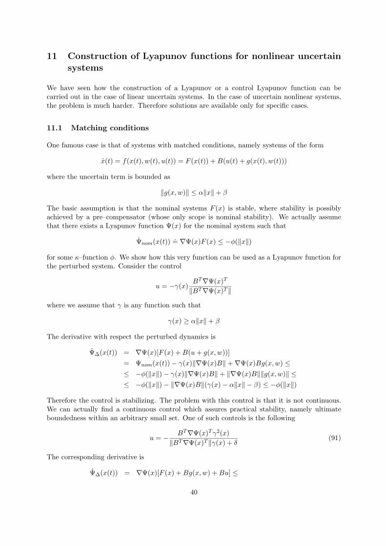
11 Construction of Lyapunov functions for nonlinear uncertain

systems

We have seen how the construction of a Lyapunov or a control Lyapunov function can becarried out in the case of linear uncertain systems. In the case of uncertain nonlinear systems,the problem is much harder. Therefore solutions are available only for specific cases.

11.1 Matching conditions

One famous case is that of systems with matched conditions, namely systems of the form

x(t) = f(x(t), w(t), u(t)) = F (x(t)) +B(u(t) + g(x(t), w(t)))

where the uncertain term is bounded as

‖g(x,w)‖ ≤ α‖x‖+ β

The basic assumption is that the nominal systems F (x) is stable, where stability is possiblyachieved by a pre–compensator (whose only scope is nominal stability). We actually assumethat there exists a Lyapunov function Ψ(x) for the nominal system such that

Ψnom(x(t)).= ∇Ψ(x)F (x) ≤ −φ(‖x‖)

for some κ–function φ. We show how this very function can be used as a Lyapunov function forthe perturbed system. Consider the control

u = −γ(x) BT∇Ψ(x)T

‖BT∇Ψ(x)T ‖

where we assume that γ is any function such that

γ(x) ≥ α‖x‖+ β

The derivative with respect the perturbed dynamics is

Ψ∆(x(t)) = ∇Ψ(x)[F (x) +B(u+ g(x,w))]

= Ψnom(x(t))− γ(x)‖∇Ψ(x)B‖+∇Ψ(x)Bg(x,w) ≤≤ −φ(‖x‖)− γ(x)‖∇Ψ(x)B‖+ ‖∇Ψ(x)B‖‖g(x,w)‖ ≤≤ −φ(‖x‖)− ‖∇Ψ(x)B‖(γ(x)− α‖x‖ − β) ≤ −φ(‖x‖)

Therefore the control is stabilizing. The problem with this control is that it is not continuous.We can actually find a continuous control which assures practical stability, namely ultimateboundedness within an arbitrary small set. One of such controls is the following

u = − BT∇Ψ(x)Tγ2(x)

‖BT∇Ψ(x)T ‖γ(x) + δ(91)

The corresponding derivative is

Ψ∆(x(t)) = ∇Ψ(x)[F (x) +Bg(x,w) +Bu] ≤

40

≤ ∇Ψ(x)F (x) + ‖∇Ψ(x)‖‖g(x,w)‖+∇Ψ(x)Bu ≤

≤ ∇Ψ(x)F (x) + ‖∇Ψ(x)B‖γ(x)− ‖∇Ψ(x)B‖2γ2(x)‖∇Ψ(x)B‖γ(x) + δ

≤ −φ(‖x‖) + δ‖∇Ψ(x)B‖γ(x)

‖∇Ψ(x)B‖γ(x) + δ

≤ −φ(‖x‖) + δ

Takeκ(δ) : min

φ(‖x‖)≥δΨ(x).

Then the state is confined in the set

S = x : Ψ(x) ≤ κ,and since κ(δ) → 0 as δ → 0, this assures practical stability.

The above control is not unique. For instance (91) can be written as

u = − γ2(x)

‖BT∇Ψ(x)Tγ(x)‖+ δBT∇Ψ(x)T = γ(x) BT∇Ψ(x)T (92)

which is a gradient–based control of the form (47). Any function γ(x) ≥ γ(x) corresponds toa suitable. Under appropriate assumptions, such as the linearity of the uncertain model, γ caneven chosen as a sufficiently large constant.

11.2 Beyond the matching conditions: Backstepping

Clearly the systems with matched uncertainty form a very special class. Let us now considera class which is more general namely that of systems in the so called Strict Feedback Form. Asystem of the form

x(t) = F (x(t), w(t)) +G(x(t), w(t))u(t)

Is said to be in the strict feedback form if it can be represented as

F (x,w) =

f11 f12 0 . . . 0f21 f22 f23 . . . 0. . . . . . . . . . . . 0

fn−1,1 fn−1,2 fn−1,3 . . . fn−1,n

fn,1 fn,2 fn,3 . . . fn,n

x+ F (0, w)

fi,j = fi,j(x1, x2, . . . , xi, w)

G(x,w) =

00:0

fn,n+1

fi,i+1 6= 0.

This structure admits a block version in which fi,i+1 are full row rank matrices. The basicidea here is the following. For a system in the form above, any variable xi+1 can be seen as a“virtual” control signal for the subsystem associated with the variables xi. Under appropriateassumptions (for instance that the functions fi,j are all bounded) we can stabilize this system.We present the idea by means of an example.

41

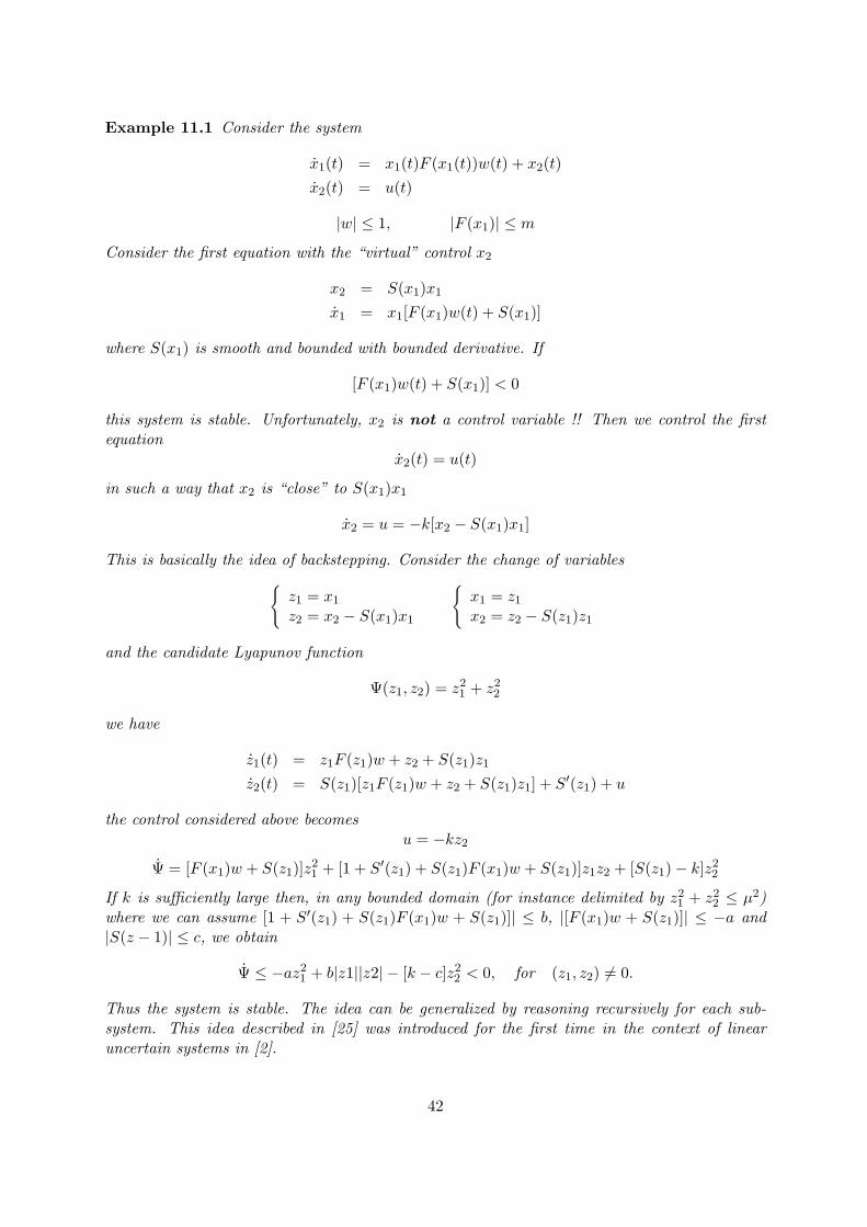
Example 11.1 Consider the system

x1(t) = x1(t)F (x1(t))w(t) + x2(t)

x2(t) = u(t)

|w| ≤ 1, |F (x1)| ≤ m

Consider the first equation with the “virtual” control x2

x2 = S(x1)x1

x1 = x1[F (x1)w(t) + S(x1)]

where S(x1) is smooth and bounded with bounded derivative. If

[F (x1)w(t) + S(x1)] < 0

this system is stable. Unfortunately, x2 is not a control variable !! Then we control the firstequation

x2(t) = u(t)

in such a way that x2 is “close” to S(x1)x1

x2 = u = −k[x2 − S(x1)x1]

This is basically the idea of backstepping. Consider the change of variables

z1 = x1z2 = x2 − S(x1)x1

x1 = z1x2 = z2 − S(z1)z1

and the candidate Lyapunov function

Ψ(z1, z2) = z21 + z22

we have

z1(t) = z1F (z1)w + z2 + S(z1)z1

z2(t) = S(z1)[z1F (z1)w + z2 + S(z1)z1] + S′(z1) + u

the control considered above becomesu = −kz2

Ψ = [F (x1)w + S(z1)]z21 + [1 + S′(z1) + S(z1)F (x1)w + S(z1)]z1z2 + [S(z1)− k]z22

If k is sufficiently large then, in any bounded domain (for instance delimited by z21 + z22 ≤ µ2)where we can assume [1 + S′(z1) + S(z1)F (x1)w + S(z1)]| ≤ b, |[F (x1)w + S(z1)]| ≤ −a and|S(z − 1)| ≤ c, we obtain

Ψ ≤ −az21 + b|z1||z2| − [k − c]z22 < 0, for (z1, z2) 6= 0.

Thus the system is stable. The idea can be generalized by reasoning recursively for each sub-system. This idea described in [25] was introduced for the first time in the context of linearuncertain systems in [2].

42

Let us show how the idea can be extended to the n–dimensional case. For brevity, we workunder special assumption that can be easily removed. We assume that the system has a scalarinput. Furthermore we assume that the functions fi,j are all bounded as |fi,j | ≤ Mi,j and thatthe fi,i+1 are bounded away from zero (without restriction we assume all of them positive)fi,i+1 ≥ Ni. We assume also that F (0, w) = 0. Then we can proceed as follows. Consider thefollowing “immersion”

x = F (x,w)x+G(x,w)u ∈ Ax+Bu, A ∈ A, and B ∈ B

where A and B are the set of interval matrices of the form

A =

a11 a12 0 . . . 0a21 a22 a23 . . . :. . . . . . . . . . . . 0

an−1,1 an−1,2 an−1,n−1 . . . an−1,n

an,1 an,2 an,3 . . . an,n

, and B =

00:0

an,n+1

such that|ai,j | ≤Mi,j , and bi,i+1 ≥ Ni

The elements of the form ai,i+1 have a bar to remind that they are non–zero. This kind ofimmersions will be discussed later. Consider the following change of variables.

z =

1 0 . . . . . . 0k1 1 0 . . . 0k1k2 k2 1 . . . 0: : : : :

k1 . . . kn−1 . . . . . . kn−1 1

x, x =

1 0 . . . . . . 0−k1 1 0 . . . 00 −k2 . . . . . . 0: : : 1 :0 . . . . . . −kn−1 1

z

where ki are design parameters. It is not difficult that with such a change of variables, and thefeedback

u = −knzn(t)B remains unchanged while the the closed loops state matrix becomes

ACL(k) =

a11 − a12k1 a12 0 · 0a21(k1) a22(k1)− a23k2 a23 · 0

a3,1(k1, k2) a3,2(k1, k2) a3,3(k1, k2)− a3,3k3 · :. . . . . . . . . · an−1,n

an,1(k1, . . . , kn−1) an,2(k1, . . . , kn−1) . . . · an,n(k1, . . . , kn−1)− an,nkn

where all entries aij are functions of the original parameter and the coefficients ki. Now it isfundamental to note that

ai,j = ai,j(k1, k2, . . . , ki−1)

and then in the ith row the elements are functions only of the previous parameters, with theexception of the diagonal elements which contain the terms ai,i+1ki. The proof now proceeds byshowing that by an appropriate choice of the parameters k1, k2, . . . kn, this system admits thequadratic Lyapunov function Ψ(z) = zT z which is equivalent to show that Q(K) = ACL(K)T +ACL(K) is a negative definite matrix. Note that such a a matrix is of the form

Q(K) =

43

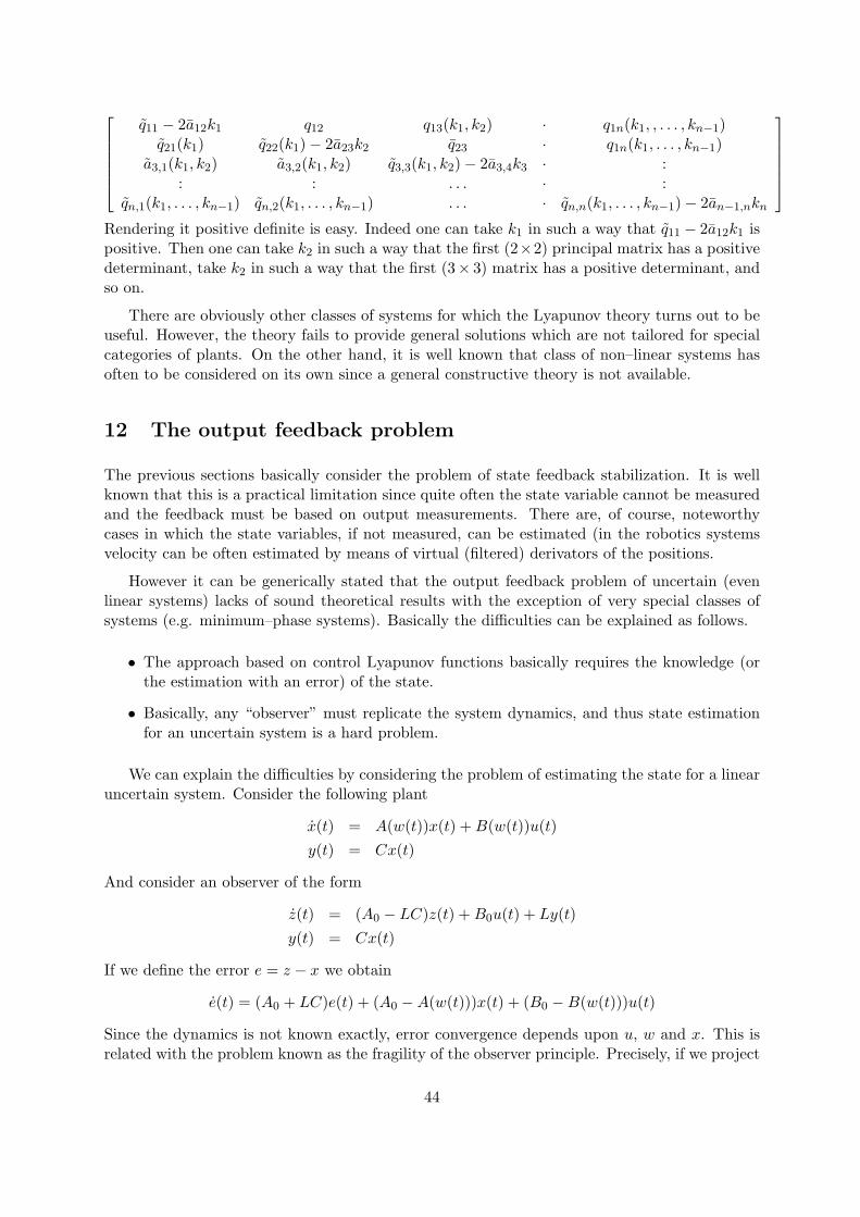
q11 − 2a12k1 q12 q13(k1, k2) · q1n(k1, , . . . , kn−1)q21(k1) q22(k1)− 2a23k2 q23 · q1n(k1, . . . , kn−1)

a3,1(k1, k2) a3,2(k1, k2) q3,3(k1, k2)− 2a3,4k3 · :: : . . . · :

qn,1(k1, . . . , kn−1) qn,2(k1, . . . , kn−1) . . . · qn,n(k1, . . . , kn−1)− 2an−1,nkn

Rendering it positive definite is easy. Indeed one can take k1 in such a way that q11 − 2a12k1 ispositive. Then one can take k2 in such a way that the first (2×2) principal matrix has a positivedeterminant, take k2 in such a way that the first (3× 3) matrix has a positive determinant, andso on.

There are obviously other classes of systems for which the Lyapunov theory turns out to beuseful. However, the theory fails to provide general solutions which are not tailored for specialcategories of plants. On the other hand, it is well known that class of non–linear systems hasoften to be considered on its own since a general constructive theory is not available.

12 The output feedback problem

The previous sections basically consider the problem of state feedback stabilization. It is wellknown that this is a practical limitation since quite often the state variable cannot be measuredand the feedback must be based on output measurements. There are, of course, noteworthycases in which the state variables, if not measured, can be estimated (in the robotics systemsvelocity can be often estimated by means of virtual (filtered) derivators of the positions.

However it can be generically stated that the output feedback problem of uncertain (evenlinear systems) lacks of sound theoretical results with the exception of very special classes ofsystems (e.g. minimum–phase systems). Basically the difficulties can be explained as follows.

• The approach based on control Lyapunov functions basically requires the knowledge (orthe estimation with an error) of the state.

• Basically, any “observer” must replicate the system dynamics, and thus state estimationfor an uncertain system is a hard problem.

We can explain the difficulties by considering the problem of estimating the state for a linearuncertain system. Consider the following plant

x(t) = A(w(t))x(t) +B(w(t))u(t)

y(t) = Cx(t)

And consider an observer of the form

z(t) = (A0 − LC)z(t) +B0u(t) + Ly(t)

y(t) = Cx(t)

If we define the error e = z − x we obtain

e(t) = (A0 + LC)e(t) + (A0 −A(w(t)))x(t) + (B0 −B(w(t)))u(t)

Since the dynamics is not known exactly, error convergence depends upon u, w and x. This isrelated with the problem known as the fragility of the observer principle. Precisely, if we project

44

an observer for an unstable system based on a nominal model, arbitrarily small perturbationscan produce a divergent error e.

It is also well known that if the observer is part of a feedback loop then infinitesimal pertur-bations are indeed tolerated, and in particular stability is preserved. But this implies that it isvirtually impossible to design an observer without a simultaneous consideration of a feedbackof the estimated state, so that it is not clear how to extend the known separation principle touncertain systems (although some results are available for classes of systems [5]

The situation is quite different for the gain–scheduling problem. It the term w(t) is unknownonly in the design stage but is available on–line then one can consider the observer

z(t) = (A(w(t))− L(w(t))C)z(t) +B(w(t))u(t) + L(w(t))y(t)

y(t) = Cx(t)

which produces the equation error

e(t) = (A(w(t)) + L(w(t))C)e(t)

It immediately shown that, for polytopic systems, the problem of designing a quadratic Lyapunovfunction along with a linear gain L reduces to the LMI problem

PAk + PLkC +ATk P + CTLT

k P = PAk +ATk P + PSk + CTST

k < 0, P > 0

where we have denoted by Sk.= PLk. There is a well–known duality in the synthesis of gain

scheduled observer and gain–scheduled stated feedback in the quadratic framework [20]. Theaspect of duality in a more general context has been investigated in [12, 14].

13 Application of Lyapunov techniques

The Lyapunov approach is undoubtedly one of the most successful in the field of control ofdynamical systems, especially from point of view of the applications. In this section we presentssome known problems which can be very effectively faced by means of the described techniques.

13.1 Controlling nonlinear systems via robust control methods

This stabilization method is based on the concept of absorbing system. Given any system of theform

x(t) = f(x(t), u(t))

we say that, this system is absorbed in the system

x(t) = F (x(t), u(t), w(t))

within domains X and U , if for all x ∈ X and u ∈ U

f(x, u) = F (x, u, w), for some w ∈ W, (i.e.f(x, u) ∈ F (x, u, w), w ∈ W)

This means that all the trajectories of the first system are included among the trajectories of thesecond one. Therefore stabilizing the latter implies stabilizing the former. Clearly the second

45

system should have “nice” properties. In particular, the usual trick is basically a bargain ofnonlinearity for uncertainty. Consider for instance the system

x(t) = f(x(t)) +Bu(t) (93)

and assume thatf(x) = A(w)x, w = w(x), with A(w) ∈ A

then, if the control u = Φ(x) stabilizes

x(t) = A(w(t))x(t) +Bu(t)

for all A(w(t)) ∈ A, then it stabilizes (93). Clearly the technique is useful if A is a set of simplerepresentation, for instance when

f(x) ∈ convAi x,so that

A =

A(w) =r∑

k=1

wiAi,r∑

k=1

wi = 1, wi ≥ 0

One way to create the set A is the following. Consider any component of f and assume that itis continuously differentiable inside a convex domain X . Then we can write the following

fi(x1, x2, . . . , xn) = fi(x1, x2, . . . , xn) +

∫ x

x

n∑

j=1

∂fi∂xj

(x1, x2, . . . , xn)dxj

If we assume that x is an equilibrium point we get fi(x1, x2, . . . , xn) = 0. This can be writtenas

fi(x1, x2, . . . , xn) =n∑

j=1

aij(x1, x2, . . . , xn)(xj − xj)

where aij is the “average” value. Now if we are able to provide bounds to the componentsaij(x1, x2, . . . , xn),

a−ij ≤ aij(x1, x2, . . . , xn) ≤ a+ij

we can merge the original systems in an interval time–varying system

x(t) = A(t)x(t) +Bu(t), with a−ij ≤ aij(t) ≤ a+ij

The robust stabilizability of this system implies the stabilizability of the original system (butthe opposite is not true in general).

This technique can be extended also to the case in which the control does not enter linearlyin the system. It is also immediately noticed that bounded uncertainties in the original modelcan be also faced without special difficulties.

Example. Consider the following simplified equation of a magnetic levitator

y(t) = −k i(t)2

y(t)2+ g = f(y(t), i(t))

shown in Fig. 6. Where y is the distance of a steel ball from a controlled magnet and i is thecurrent impressed by an amplifier. Let (y, i) the positive values such that f(y, i) = 0 It can bewritten as follows

f(y, u) =

∫ (y,i)

(y,i)

[

2ki2

y3dy − 2ki

y2di

]

46

Figure 6: The magnetic levitator

Now it is reasonable (in practice necessary for this system) to assume bounds on the variablessuch as

0 < y− ≤ y ≤ y+, 0 < i− ≤ i ≤ i+, 0 < k− ≤ k ≤ k+.

Then we get the absorbing model

y(t) = a(t)(y(t)− y)− b(t)(i(t)− i) (94)

with2k−i−

2

y+3 ≤ a(t) ≤ 2k+i+2

y−3 ,2k−i−

y+2 ≤ b(t) ≤ 2k+i+

y−2

13.2 Observer design for nonlinear systems by means of robust control algo-

rithms

Let us now consider a nonlinear system of the form

x(t) = f(x(t)) +Bu(t)

y(t) = Cx(t)

and let us consider an observer of the form

z = f(z(t)) + L(y − Cz) +Bu (95)

and the corresponding error equation

e = [f(e+ x)− f(x)] + LCe (96)

47

where e(t) = z(t) − x(t). Under appropriate assumptions, such as the smoothness of f we canwrite, for any x the following equation

[f(e+ x)− f(x)] = Ae, A ∈ A,

where A is a bounding set in the n × n matrices. By means of the same consideration of theprevious subsection, set A can be any set with the property that

∂f

∂x∈ A

Then, the error equation can be absorbed in the following equation.

e = (A(t)− LC)e, A(t) ∈ A (97)

If this system is is robustly stable, then also the previous error equation (96) is such thate(t) → 0.

A fundamental point is the following. The procedure for the observer design is quite similarto that of the state feedback synthesis. Actually one can see that (97) is the dual equation of

x(t) = (A(t)−BK)x(t)

that can be faced for instance by means of LMI techniques. The substantial difference is thatno uncertainties are tolerated in the original plant because we must construct the observer (95),tha could not be done , unless the uncertain parameters are measured on–line by the controller.

Another interesting case is that of systems of the form

x1(t) = f11(x1(t)) + f12(x1(t))x2(t) + g1(x1(t))u(t)

x2(t) = f21(x1(t)) + f22(x1(t))x2(t) + g2(x1(t))u(t)

y(t) = x1(t)

where x1 ∈ IRn1 x2 ∈ IRn2 , x1 + x2 = n. The peculiarity of this system is that the unmeasuredvector x2 enters in an affine way in the equations. For this system it is possible to determine areduced–order observer as follows. Define the variable

w(t) = x2(t)− Lx1(t)

where matrix L is a design parameter. Then we have

w = (f22(x1)− Lf12)x2 + f21(x1)− Lf11(x1) + (g2(x1)− Lg1(x1))u

± (Lf12(x1)L− f22(x1)L)

= (f22(x1)− Lf12(x1))w

+ [f21(x1)− Lf11(x1) + f22(x1)L− Lf12(x1)L] + [g2(x1)− Lg1(x1)]u︸ ︷︷ ︸

.=ρ(x1,u)

For the resulting systemw = (f22(x1)− Lf12(x1))w + ρ(x1, u)

we consider the reduced observer

zw = (f22(x1)− Lf12(x1))zw + ρ(x1, u)

48

If we consider the error e = zw − w = z2 − x− 2, we have that its evolution is governed by

e = (f22(x1)− Lf12(x1))e

Therefore, if under appropriate assumptions we can find L for which this system is stable, wecan asymptotically estimate x2.

This kind of tricks can be used even with other classes of systems for instance not necessarilyu-affine as in the next example.

Example 13.1 Consider a system of the form

x1 = x2

x2 = f(x1, u)

where y = x1 is the measured variable. This is the the typical equation of a mechanical systemincluding the levitator. Define w = x2 − Lx− 1 to derive

w = −Lw + f(x1, u)− L2x1

for which we can construct the observer

zw = −Lzw + f(x1, u)− L2x1

Note that this observer is tolerant against small variations of the model f . Indeed, if the modelis not accurate so that the true system is x2 = f(x1, u) + ∆ the error equation becomes

e = −Le+∆

which is small as long as ‖∆‖ is small.

13.3 Domain of attraction

A classical application of the Lyapunov theory is the determination of a domain of attraction[26]. Let us consider the basic idea beyond the technique. Assume that the system

x(t) = f(x(t))

with f(0) = 0 is locally stable and its linerization admits a local Lyapunov function Ψ(x). Thenas already mentioned, there exists a positive value κ such that N [Ψ, κ] is a domain of attraction.The problem is how to determine one of such κ. Such a number κ must be such that

maxκ : N [Ψ(x), κ] ⊂ N [Ψ(x), 0]

This can be achieved by considering the following problem

κ = minΨ(x) ≥ δ : Ψ(x) = 0 − ǫ

where the small numbes δ > 0 and ǫ > 0 are necessary to eliminate the trivial solution at theorigin and to avoid points with zero derivative. It is obvious that if the system is uncertainx = f(x,w), then the problem can be modified as follows. Define (with an abuse of notation)

Ψmax(x) = maxw∈W

Ψ(x,w).

49

Thenκ = minΨ(x) ≥ δ : Ψmax(x) = 0 − ǫ

The choice of the function Ψ basically fixes the “shape” of the domain. Unfortunately this choiceis critical as shown in the next example.

Example 13.2 Consider the following system

x1(t) = −[x1(t)− x31(t)]− x2(t)

x2(t) = x1(t)− x2(t)

and the functionΨ(x) = x21 + x22

So thatΨ(x) = −2x21 − 2x22 + 2x41

it is easy to see that as ǫ → 0 κ → 1. So the corresponding domain is the unit circle (see Fig.7). A different possibility is the following. Write the nonlinearity between square brackets as

−[x1(t)− x31(t)] = −[1− w]x1, with w = x21

Now if we impose bounds of the form|x1| ≤ x1 (98)

we have|w| ≤ w =

√x1 (99)

Then we can consider the uncertain linear systems with matrix

A(w) =

[

−[1− w] −11 −1

]

and compute the largest domain of attraction subject to the constraints (98) and (99). In Figure7, this domain is computed for x1 = 3/2 and w =

√

3/2 by means of a polyhedral Lyapunovfunctions. The vertices of the unit ball are denoted by “*”. The “true” domain of attractionhas been also represented by means of several trajectories by backward integration starting fromseveral initial conditions inside the previous domain of attractions. Clearly this example showthe limits of the determination of the domain of attraction achieved by guessing the shape of thefunction or by the merging in an uncertain system.

13.4 High gain adaptive control

An interesting application associated with a control Lyapunov function is the so called high–gainadaptive control. Consider, for instance, an uncertain system which is control–affine and withconstant and certain input matrix.

x(t) = f(x(t), w(t)) +Bu(t), w(t) ∈ W

and assume that a control Lyapunov function Ψ is given. We have seen that, if Ψ is smooth, acontroller can be given in the form

u(t) = −γBT∇Ψ(x) (100)

50

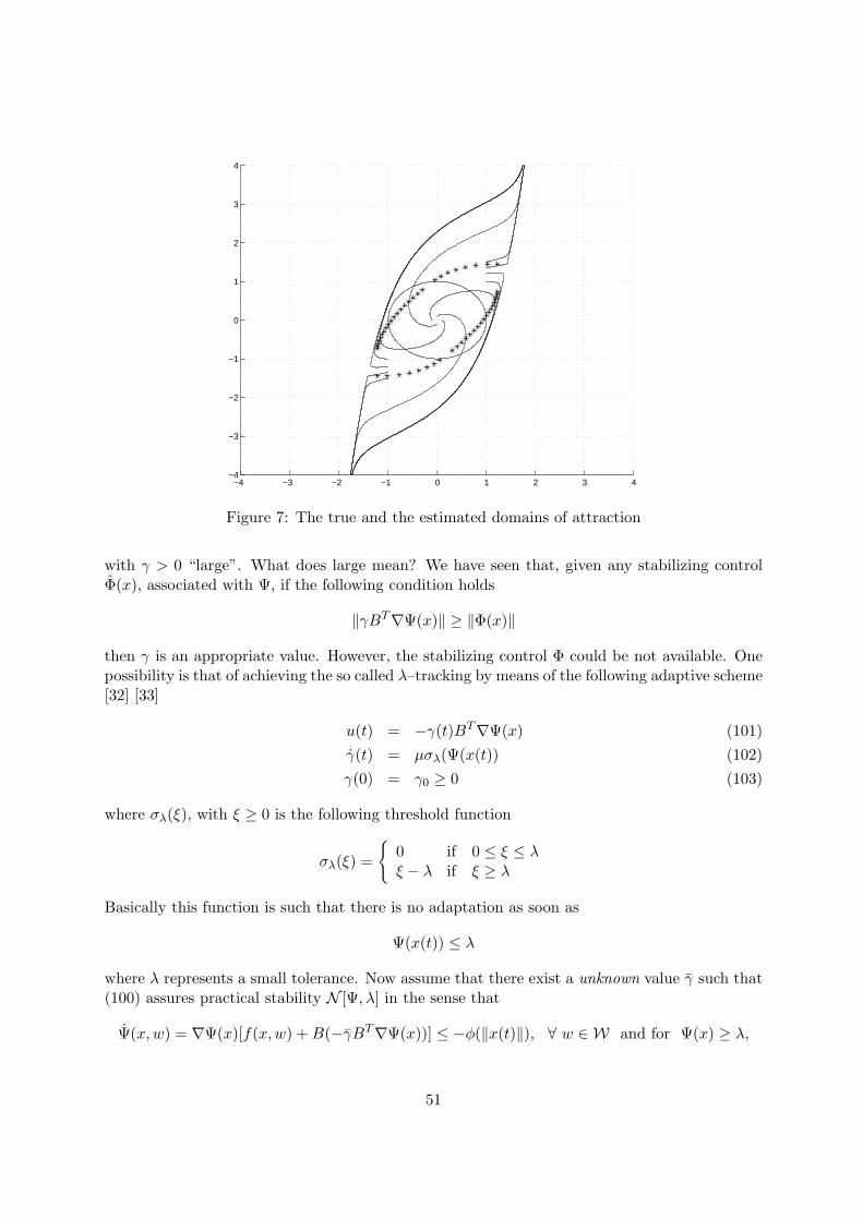
−4 −3 −2 −1 0 1 2 3 4−4

−3

−2

−1

0

1

2

3

4

Figure 7: The true and the estimated domains of attraction

with γ > 0 “large”. What does large mean? We have seen that, given any stabilizing controlΦ(x), associated with Ψ, if the following condition holds

‖γBT∇Ψ(x)‖ ≥ ‖Φ(x)‖

then γ is an appropriate value. However, the stabilizing control Φ could be not available. Onepossibility is that of achieving the so called λ–tracking by means of the following adaptive scheme[32] [33]

u(t) = −γ(t)BT∇Ψ(x) (101)

γ(t) = µσλ(Ψ(x(t)) (102)

γ(0) = γ0 ≥ 0 (103)

where σλ(ξ), with ξ ≥ 0 is the following threshold function

σλ(ξ) =

0 if 0 ≤ ξ ≤ λξ − λ if ξ ≥ λ

Basically this function is such that there is no adaptation as soon as

Ψ(x(t)) ≤ λ

where λ represents a small tolerance. Now assume that there exist a unknown value γ such that(100) assures practical stability N [Ψ, λ] in the sense that

Ψ(x,w) = ∇Ψ(x)[f(x,w) +B(−γBT∇Ψ(x))] ≤ −φ(‖x(t)‖), ∀ w ∈ W and for Ψ(x) ≥ λ,

51

As we have seen the same inequality is verified for any γ ≥ γ. Then the adaptive scheme(101)–(102) converges in the sense that as t→ ∞

γ(t) → γ∞ <∞, (104)

σλ(Ψ(x(t))) → 0. (105)

then the gain is asymptotically finite and Ψ(x(t)) is asymptotically smaller or equal to λ.

The significance of this approach can be explained in the next points.

• It solves the problem due to the ignorance of γ.

• It avoids too large values of γ since the adaptation stops as soon as the condition Ψ(x) ≤ λis satisfied.

In particular the last condition is important because too large values of γ imply excessive controlexploitation and, as it is know, can excite high–frequency neglected dynamics and produceinstability.

This kind of scheme works under appropriate minimum–phase and relative degree assump-tions in the case of output feedback.

Example 13.3 Consider the following system

x1(t) = x2(t)

x2(t) = w(t)sin(x1(t)) + u(t)

with|w| ≤ w

and the control–Lyapunov function Ψ(x1, x2) =12 x

TPx with

P =

[

2 11 2

]

the corresponding control is then

u(t) = −γ(t)BTPx = −γ(t)(x1 + 2x2)

To show that Ψ is a control Lyapunov function it is sufficient to consider its Lyapunov derivative.Simple computations yield

Ψ(x, γ) = −γx21 + (2− 4γ)x1x2 − (4γ − 1)x22 + (x1 + 2x2)wsin(x1) (106)

≤ −γx21 + (2− 4γ)|x1||x2| − (4γ − 1)x22 + wx21 + w|x1||x2| (107)

= −(γ − w)x21 + 2(1 + w − 2γ)|x1||x2| − (4γ − 1)x22 < 0 (108)

for γ > large enough (the last inequality is simply derived by checking the nature of the quadraticform). Figure 8 shows the variables x1, x2 and the gain γ(t) with µ = 1 and λ = 0.01. In thiscase we obtained the limit value κ∞ = 14.93.

52

0 1 2 3 4 5 6 7 8 9 10−2

0

2

4

6

8

10

12

14

16

Figure 8: The gain evolution (upper curve) and the state evolution

13.5 Constrained control

It is well known that one of the most crucial problems in the applications is the presence of hardconstraints on both the state and input variables. The Lyapunov theory offers an interestingpoint of view for the problem [37]. Assume that constraints of the form

x(t) ∈ X , u(t) ∈ U ,

with X and U including the origin as an interior point, are assigned. Given any stabilizingcompensator, it is know that, in general, such constraints can be satisfied only if the state isclose enough to the origin. Therefore the typical problem is that of evaluating the set of initialconditions from which the constraints are not violated. Assume that there exists a controlLyapunov function Ψ(x) associated with a control u = Ψ(x). Consider the control–admissibleset

Xu = x : Φ(x) ∈ Uand consider any value κ such that

N [Ψ, κ] ⊆ Xu

⋂

X

then any state x(0) ∈ N [Ψ, κ] is such that

x(t) ∈ X

u(t) ∈ Ufor all t ≥ 0. In few words N [Ψ, κ] becomes a safety set in the sense that any trajectory startinginside it will not violate the constraints.

53

Let us consider now the case of a linear system

x(t) = A(w(t))x(t) +B(w(t))u(t),

A(w) =s∑

i=1

wiAi,s∑

i=1

wi = 1, wi ≥ 0,

B(w) =s∑

i=1

wiBi,s∑

i=1

wi = 1, wi ≥ 0,

And assume for instance that a linear quadratic stabilizing controller u = Kx has been com-puted. Assume that U is the unit ball of the ∞–norm (namely that the constraints are |ui| ≤ 1.Then

Xu = x : ‖Kix‖∞ ≤ 1It is easy to compute an ellipsoidal set of the form

E = x : xTPx ≤ 1

which is invariant and included in Xu. Indeed denoting by Q = P−1 we have that E ⊆ Xu if andonly if

kiQkTi ≤ 1 (109)

Let Ai = Ai +BiK, then the invariance condition for E is

QATi + AiQ < 0 (110)

Then (109) and (110) form a convex set in the parameter Q. One therefore can optimize the sizeof this set for instance the volume (see [20]) for further details.

It is known that determining a domain of ellipsoidal domain of attractions is not efficientin terms of the accuracy of the representation since the actual stability domain can be quitelarger than the derived one. Other type of domains of attraction can be determined by means ofpolyhedral Lyapunov functions using a procedure similar to that previously described. In thiscase, the advantage is that for linear (even uncertain) systems with linear constraint the largestadmissible domain can be arbitrarily closely approximated by a polyhedron and therefore thepolyhedral functions are non–conservative from this point of view. If we have uncertain nonlinearsystems the domain of attraction is in general non–convex and in general very hard to determine.However, an approximated solution can be derived by considering absorbing equations as in thefollowing example.

Example 13.4 Let us consider the magnetic levitator of Figure 6 and the “absorbing” equation(94). The corresponding matrices are

A =

[

0 1a 0

]

B =

[

0−b

]

with1507 ≤ a ≤ 2177, 17.8 ≤ b ≤ 28

We have considered the control action

u = 120(0.025x1 + 0.022x2)

54

A feasible initial condition set corresponding to |u| ≤ 0.5 is the polygon whose vertices are thecolumns of the matrix [X,−X] where X is reported next

X =

[

0.005 0.0050 −0.398

]

In Figure (9) the estimated and the “true” safety set are reported. The “true” region is estimatedfor the nonlinear model (assuming known parameters) by integrating the full force trajectories.

position

Speed

ma

gn

et

0 .5 1.5

Figure 9: The estimated (polygonal) and the true and safety regions

13.6 Robot Manipulators

Robotics is one of the most popular application field of control theory. Before considering aspecific application let us consider the following result concerning the presence of uncertainty inthe input channel. Consider the system

x(t) = f(x(t), w(t)) +B(I +∆B)u (111)

where ∆B(x(t), w(t)) represents a matched uncertainty. Assume that Ψ(x) is a control Lyapunovfunction with the control

u = −γBT∇Ψ(x)T

(possibly outside a certain neighborhood S) for the system with ∆B = 0. Then it is also aControl Lyapunov function for the system (111) provided that

∆TB∆B < λ2I, with λ < 1. (112)

Indeed, consider the Lyapunov derivative

Ψ(x) = ∇Ψ(x)f(x(t), w(t))− γ∇Ψ(x)BBT∇Ψ(x)T − γ∇Ψ(x)B∆BBT∇Ψ(x)T =

= ∇Ψ(x)f(x(t), w(t))− (1− λ)γ∇Ψ(x)BBT∇Ψ(x)T −γ∇Ψ(x)B(λI −∆B)BT∇Ψ(x)T

︸ ︷︷ ︸

≤0

≤ ∇Ψ(x)f(x(t), w(t))− γ∇Ψ(x)BBT∇Ψ(x)T

55

where γ = (1 − λ)γ. then, for large enough we have Ψ(x) ≤ −φ(‖x‖), for some κ–function φby assumption. Therefore the prize to contrast ∆B is to increase γ as γ = γ/(1 − λ). It is notdifficult to see that if γ(x) (and then γ(x)) are functions of x, the property still holds.

Let us consider now the typical equation of a robotic manipulator.

M(q(t))q(t) +H(q(t), q(t))q(t) +G(q(t)) = τ(t) (113)

where q(t) represents the free parameters m-vector, q(t) the corresponding velocity vector and τis the torque vector. The mass matrix M(q) is assumed invertible for all q A typical procedureto design a control is that of considering a pre–compensator of the form

τ(t) =M(q)u(t) +H(q, q)q +G(q) (114)

so that the resulting system isM(q(t))[q(t)− u(t)] = 0

In view of the invertibility of M(q) this system is equivalent to the m decoupled equations

qi(t) = ui(t),

whose control is an elementary task.

The problem with this standard procedure is that the control (114) cannot be implementedbecause the model is uncertain and the true pre–compensator is based on a approximated model

τ = M(q)u(t) + H(q, q)q + G(q) (115)

If we apply the control (115) the resulting equation becomes

q(t) = u+M(q)−1[M(q)−M(q)]︸ ︷︷ ︸

∆B

u(t) +

+ M(q)−1[H(q, q)−H(q, q)]q +M(q)−1[G(q)−G(q)]︸ ︷︷ ︸

∆f

or, in a simpler formq(t) = [I +∆B]u(t) + ∆f (116)

Now, under the assumption that M(q) is a sufficiently accurate estimate of the mass matrixM(q) we can assume that

∆B =M−1(M −M) (117)

satisfies (112), along with the following boundedness condition for ∆f

‖∆f (q, q)‖ ≤ α+ β‖x‖. (118)

Then the the next deign procedure can be used.

Procedure 13.1

1. Assume ∆B = 0 and ∆f = 0 and consider nominal system whose state vector is x =[qT , qT ]T by setting

A =

[

0 I0 0

]

B =

[

0I

]

56

2. Find a control Lyapunov function associated with the matrix P > 0, by considering theequation

QAT +AQ+RTBT +BR = −S < 0

where Q = P−1 (see Subsection 8.2) and consider the state feedback controller

u(t) = −γBTPx(t)

which stabilizes the nominal system with γ = 1.

3. Assure uniform ultimate boundedness for the actual plant by taking γ large enough.

The fact that such a large γ, as required in the last step of the procedure, exist can be explainedsince in view of the bound (118) and (117). First assume ∆B = 0. By elementary analysis onecan show that

α‖BTSx‖ − γ‖BTSx‖2 ≤ α

2γ.

Fix any small ǫ and consider the ǫ-ellipsoid

E = x : xTPx ≤ ǫ.Let γǫ such that, for all states in the complement x 6∈ E

xTSx

2≥ α

2γǫ.

Denoting by σmin(S) the smallest eigenvalue of S, we get for x 6∈ EΨ(x) = −xTSx+ xTSB∆f − γxTSBBTSx

≤ −xTSx+ α‖BTSx‖+ β‖BTSx‖‖x‖ − γ‖BTSx‖2 == −xTSx/2 + β‖BTSx‖‖x‖ − (γ − γǫ)‖BTSx‖2+ −xTSx/2 + α‖BTSx‖ − γǫ‖BTSx‖2

︸ ︷︷ ︸

≤0

≤ −σmin(S)‖x‖2/2 + β‖BTSx‖‖x‖ − (γ − γǫ)‖BTSx‖2.The last expression is a quadratic form in the variables ‖x‖ and ‖BTSx‖ and by taking γ largeenough, we can render it negative definite. Then if we have (117), we can take γ = γ/(1− λ) asshown at the beginning of the subsection.

The practical problem is that of determining the bounds (118) (117). However it is funda-mental to establish that, for γ large enough, the system is asymptotically driven in the ellipsoid,then adaptive scheme proposed in section 13.4 is very useful.

Let us finally consider an extended model of a manipulator with elastic joints. A typicalapproximation is to model the elasticity as linear springs at the joints. The resulting model isof the form

D(q2)q2 + C(q1, q1)q1 + g(q1) +K(q1 − q2) = 0

Jq2 +K(q2 − q1) = τ

It is not difficult to see that this model, if written in terms of first order equations, is in a(multi–input) strict feedback form. For more details on this problem the reader is referred tothe paper [53] and the reference inside.

57

13.7 Switching systems

A recent field in which the Lyapunov theory has been exploited is the analysis and control ofswitching systems [40]. A switching system is a system of the form

13.8 Switching systems

x(t) = f(x(t), u(t), q(t))

withq(t) ∈ Q,

where Q is a finite set. Typically the following three important cases have to be considered forthe switching signal q(t)

• q(t) is an uncontrolled (exogenously determined) unknown to the controller;

• q(t) is an uncontrolled (exogenously determined) but known to the controller;

• q(t) is a controlled switching signal;

Let us first consider the case in which the system is uncontrolled and there is no input signalu(t). If we are interested in a Lyapunov function Ψ for the system

x(t) = f(x(t), p(t))

the we have to cope with the condition

Ψ(x, p) = ∇Ψ(x)f(x, p) ≤ −φ(‖x‖). ∀p ∈ P

Without restriction assume that p is an index belonging to a finite set 1, 2, . . . , NP . Then thefunction Ψ satisfies the previous condition if and only if it satisfies the condition

Ψ(x, α) =

Np∑

p=1

αp ∇Ψ(x)f(x, p) ≤ −φ(‖x‖)

with∑Np

p=1 αp = 1, and αp ≥ 0. In particular, in the linear case, the stability of the switchingsystem

x(t) = Apx(t)

is equivalent to the stability of the polytopic system x(t) = [∑Np

p=1 αpAp] x(t), and then analyzedas previously described.

The situation is completely different when the switching is controlled. In this case thenegativity of the Lyapunov derivative has not to be satisfied for all p ∈ P but for some p. Atypical sufficient condition for this condition to be achieved is the following: assume that thereexists a Lyapunov stable system in the convex hull of the points f(x, p), precisely there exists asystem

x(t) = f(x)

such thatf(x) ∈ convf(x, p), p = 1, 2, . . . , Np

58

and that admits a Lyapunov function

∇Ψ(x)f(x) ≤ −φ(‖x‖)then there exists a stabilizing switching strategy of the form

p = Φ(x) = argminp

∇Ψ(x)f(x, p)

Indeed it is immediately seen that

minp

∇Ψ(x)f(x, p) ≤ ∇Ψ(x)f(x) ≤ −φ(‖x‖)

In the case of a linear plantx(t) = Aix(t), 1 = 1, 2, . . . , r

the problem is easily solved if there exists

A ∈ convAiwhich is stable. Consider any Lyapunov function for the system x = Ax, i.e. a symmetricpositive definite matrix P such that

ATP + PA ≤ −xTQx, Q > 0

Then the switching law is

Φ(x) = argmini

Ψ(x) = argmini

xTPAix,

which assures the conditionΨ(x) ≤ −xTQx

Unfortunately the existence of such a stable element of the convex hull is not necessary. Forinstance the system given by the pair of matrices

A(w) =

[

0 1−1 + w −a

]

where a < 0 is not stable for any value of a. w = ±w is a switching parameter. However, if a issmall enough then there exists a suitable stabilizing strategy.

Let us now consider the problem of stabilization of the continuous time linear system

x(t) = Aix(t) +Biu(t)

Again, if the switching is uncontrolled (known or unknown to the controller), then the problemcan be faced by finding a common control Lyapunov function. The case of controlled switchingcan be faced as follows. Assume that in the convex hull of the systems there is a stabilizablesystems

[A, B] = [s∑

i=1

wiAi,s∑

i=1

wiBi],s∑

i=1

wi = 1, wi ≥ 0.

and consider a stabilizing feedback u = Kx. Then

A+ BK =s∑

i=1

wi[Ai + KBi] =s∑

i=1

wi[Ai]

is stable and therefore there exists a switching strategy which stabilizes the system. As we haveobserved before, this solution is conservative.

A typical example of application is a system with quantized control.

59

Example 13.5 The following model represents the two–tank hydraulic system shown in Figure10.

h1(t) = −α√

x1(t) + h1 − x2(t)− h2 + u(t) + q

h2(t) = α√

x1(t) + h1 − x2(t)− h2 − β√

x2(t) + h2

where α and β are unknown positive parameters and where h1, h2 and q are the steady–statewater levels and incoming flow satisfying the conditions

h1 =

(q

α

)2

+

(q

β

)2

, h2 =

(q

β

)2

.

Figure 10: The two–tanks hydraulic system

Let us now consider the candidate control Lyapunov function

Ψ(x) =1

2

(

x21 + x22

)

The corresponding Lyapunov derivative for x ∈ N [Ψ, h22/2] (this value is chosen in such a waythat the ball is included in the positive region for the true levels hi + xi)

Ψ(x, u) =

= α(x1 − x2)

(√

x1(t) + h1 − x2(t)− h2 − q

)

+ x2

(

β√

x2(t) + h2 − q

)

︸ ︷︷ ︸.=φN (‖x‖)

+x1u ≤

− φN (x1, x2) + x1u

Note that −φN (x1, x2), the natural derivative achieved for u = 0, is negative definite, which con-firms the system stability. Note that this is true for the nonlinear dynamics inside the consideredregion.

60

Now let us assume that the control input admits three admissible values

u(t) ∈ −q; 0, q

which correspond to the three cases in which none, just one or both the switching valves are open.

However, to assure a certain degree of contractivity, one can use the following switchingcontrol law

u = −q sgn(x1)which renders the convergence to the equilibrium much faster. Clearly if α and β may vary,this produces an offset. It can be shown that, with the considered control, only the offset on thesecond tank x2 6= 0 is possible.

As it is known, from a practical point of view, the discontinuous controller has to implementedwith a threshold. We actually consider the function

u =

−q sgn(x1) if |x1| > ǫ0 if |x1| ≤ ǫ

In Figures 11 and 12 show the experimental behavior with ǫ = 0.01 and ǫ = 0.03, being the lattermuch subject to ripples as expected.

Figure 11: The experimental behavior of the plant with ǫ = 0.01

As a final comment, the reader might be interested in understanding how the candidate Lya-punov functions has been chosen. The answer is that the linearized model in the equilibriumpoint admits a state matrix which is stable and symmetric. This implies that ‖x‖2 is a Lya-punov function for the linearized natural dynamic.

61

Figure 12: The experimental behavior of the plant with ǫ = 0.03

13.9 Control of dynamical networks

Consider a class of dynamical networks modeled as follows

x(t) = Sg(x(t)) +Rh(x(t)) +Bu(t) + d(t), (119)

where x(t) ∈ IRn is the state, representing buffer levels, u(t) ∈ IRm is the control input, rep-resenting controlled flows, d(t) ∈ IRn is an exogenous signal, representing the demand. Vectorfunctions g and h represent natural flows between two nodes within the system. Applicationexamples include flowing of data, fluids and chemical reaction networks. A simple example isgiven by the two tank system previously considered.

Functions g and h have different physical meanings:

• g–type flows depend on the difference between the corresponding states

• h–type flows depend on the state of the starting node only.

For instance, in fluid systems, g–type flows between tanks depend on the fluid level in bothtanks, while h–type flows depend on the fluid level in the upper tank only (the two cases areillustrated in Fig. 13). In the two–tank system, we have one g–flow between the two tanks, oneh flow from the lower tank, one u–flow (controlled) from the external to the upper tank.

For each component of g and h, we have:

• gj = gj(xk − xl), where Skj = −1 and Slj = 1;

• hj = hj(xk), where Rkj = −1.

A graph N with n nodes can be associated with the system; we assume that S, R and B are

62

h(x )11 2

g(x − x )

12

1

x x

x

x 2

Figure 13: g–type (left) and h–type (right) flows in a fluid system.

incidence matrices: each of their columns has either two non–zero entries, equal to 1 and −1, ora single non–zero entry, equal either to 1 or to −1. These matrices correspond to the g flows,the h flows and the controlled u-flows.

g

u

u

g

d1

1g

3

2

d

2

2

1

2

3 4

1

hh

2

1

Figure 14: Graph of a network with natural dynamics (Example 13.6).

Matrix [S R B] is the overall incidence matrix of the graph representing the network. Inthe network graph, we distinguish between g–type, h–type, u–type and d–type arcs, associatedrespectively with the components of vector g (i.e., with the columns of S), of vector h (withthe columns of R), of the control vector u (with the columns of B) and of the demand vector d.In general, any arc connected with a single node of the graph represents a connection with theexternal environment. This is the case, for instance, of arcs associated with vector d.

Denoting by Mj the jth column of a matrix M , we can write, according to the flow rules,

gj = gj(−S⊤j x) and hj = hj(−R⊤

j x), (120)

where [R]ij = minRij , 0.

Example 13.6 In the network graph in Fig. 14 there are g–type flows:

g(x) = [g1(x1 − x3) g2(x1 − x2) g3(x2 − x4)]⊤

h–type flows:h(x) = [h1(x3) h2(x3)]

⊤

controlled flows:u = [u1 u2]

⊤

63

and exogenous flows:d = [d1 d2]

⊤

The system matrices are

S =

−1 −1 00 1 −11 0 00 0 1

, R =

0 01 0

−1 −10 0

, B =

1 00 00 −10 1

, R =

0 00 0

−1 −10 0

(121)

Remark 13.1 All the results in this subsection are valid for any choice of matrices S, R, andB, which are not necessarily incidence matrices.

We assume that functions gj(·) and hj(·) are smooth and have positive derivatives.

To analyze the stabilization problem, assume that the demand d is constant and that thereexists an equilibrium (x, u) corresponding to such a demand

0 = Sg(x) +Rh(x) +Bu+ d,

Without restriction we set x = 0 u = 0 and d = 0, a condition we can assure by a translation.

We assume that the control is component–wise bounded as

u− ≤ u ≤ u+. (122)

with u− ≤ 0 ≤ u+.

As a first technical result, we need to observe the following. Each component of g can beregarded as a function of a single variable gj(ξj) where ξj = xk−xl and hj(xk). Then consideringthe derivative with respect to this variable [17]

gj(ξ) =

[∫ 1

0

dgj(ξσ)

dξdσ

]

ξ = δg(ξ) ξ

and

hj(ξ) =

[∫ 1

0

dhj(ξσ)

dξdσ

]

ξ = δh(ξ) ξ

where δg(ξ) and δh(ξ) are positive functions, we assume unknown, which are bounded above andbelow (by positive numbers) in any bounded ball centered in 0. With this in mind we can write

x(t) = −S∆g(x)S⊤x−R∆h(x)R

⊤x+Bu(t), (123)

for some positive diagonal matrices ∆g(x) and ∆h(x).

We consider a saturated type of control. Define componentwise the saturation function sat(v)as follows

[sat(v)]j =

v+j if vj > v+jvj if v−j ≤ vj ≤ v+jv−j if vj < v−j

(124)

We consider the following saturated network–decentralized control ([16, 17]):

u = sat(−γB⊤x), (125)

64

where γ is a positive gain (the higher γ, the stronger the control action). This control is suitablefor applications in which the controlled flow in each link is decided based on the departure andarrival nodes.

A control similar to (125) isv = sat(−γB⊤z), (126)

where B = minB, 0, componentwise. In the strategy (126), the controlled flow in each link isdecided based on the departure node only. This control is suitable for applications such as datatransmission in which each node locally decides the outflows.

We have to notice that the saturation function, if we assume that the upper bound is positiveand the lower one negative, can be written as follows

sat(ξ) = δu(ξ)ξ

with positive δu(ξ). Hencesat(−γB⊤x) = −∆u(x)γB

⊤x, (127)

To recap, we have that in any ball centered in 0 all diagonal elements of the matrices∆g(x),∆h(x),∆u(x) are bounded by positive numbers above and below.

0 < ν ≤ [∆g(x)]k, [∆h(x)]j , [∆u(x)]h ≤ µ

We consider two cases. The first one in that in which all flows are of the g type

x(t) = Sg(x(t)) +Bu(t),

for this case we can take as Lyapunov candidate Ψ(x) = x⊤x/2. Then we get the following

Ψ(x) = −x⊤S∆g(x)S⊤x+ x⊤Bu

If we apply the saturated control

Ψ(x) = −x⊤S∆g(x)S⊤x− x⊤B∆u(x)γB

⊤x

= −x⊤[

S B][

∆g(x) 00 ∆u(x)

] [

S⊤

B⊤

]

x.= −x⊤Q(x)x

The matrix Q(x) is symmetric positive semidefinite and it is positive definite if and only if

rank[

S B]

= n

Then we have asymptotic stability if and only if this condition holds. Sufficiency is obvious.

Conversely, if the condition is not satisfied, take a vector z 6= 0 such that z⊤[

S B]

= 0.

Hence considering the Lyapunov–like function V (x) = z⊤x we get V = 0 hence

V (x(t)) = z⊤x(t) = z⊤x(0)

so stability cannot hold. In the context of fluid networks, this basically means that, if there areno connections with the external environment, one can take z⊤ = 1⊤ and then verify that theoverall quantity of fluid remains constant.

65

Let us now consider the asymmetric case. In this case, the squared euclidean norm is notsuitable. Indeed consider again the saturated control (125). We get

x(t) = −S∆g(x)S⊤x−R∆h(x)R

⊤j x−B∆u(x)γB

⊤x = −Q(x)x (128)

The problem now is that the matrix

Q(x) =[

S R B]

∆g(x) 0 00 ∆h(x) 00 0 ∆u(x)

S⊤

R⊤

B⊤

is not symmetric and −x⊤Q(x)x can be positive. However it is not difficult to see that it iscolumn-diagonally dominant. A good candidate is then the 1–norm [43, 17]. For a diagonallydominant matrix with negative diagonal elements, the 1–norm is a weak Lyapunov function.

Under proper connectivity conditions this function is a Lyapunov function whose derivativeis negative definite [43, 17]. The reader is referred to [18] for results along this line for chemicalnetworks. A switching control strategy, valid in the symmetric case, is proposed in [19].

13.10 Surge suppression in compression systems

Consider the system represented in Fig. 15 in which a compressor inflates a compressible fluid

f l o w

compressor

plenum

t hrot t le

cont rol

Figure 15: The compression system

in a plenum. We assume that the compressor works at constant angular speed and thereforeimpresses a pressure which is a function of the flow q in the pipe,

pcomp = Ψ(q)

The outgoing flow of fluid from the plenum is a function of the pressure in the plenum and ofthe throttle fraction opening a, having the form

qout = Γ(p)a,

66

where Γ(p) depends on the throttle characteristic. The overall dynamic model is

q = B[pcomp − p] = B[−p+Ψ(q)]

p =1

B[q − qout] =

1

B[q − Γ(p)a]

where q and p represent the incoming flow in the plenum and the plenum pressure, respectively.B is a constant parameter, known as Helmholtz constant.

It turns out that for large values of a the system admits a stable equilibrium, but for smallvalues, this point may become unstable and the system undergoes a limit cycle as shown in Fig.16, left (blue curve), and in Fig. 16, right, where the time evolution is represented. In Fig. 16left are also represented the typical compressor characteristics pcomp = Ψ(q) (red curve) and thevalve characteristic, qout = Γ(p)a (black curve), the intersection of which (q, p) is the equilibriumpoint.

−1 −0.5 0 0.5 1 1.5 20

0.2

0.4

0.6

0.8

1

1.2

1.4

1.6

1.8

2

0 5 10 15 20 250

0.2

0.4

0.6

0.8

1

1.2

1.4

1.6

1.8

2

Figure 16: The compression system without control

Let us introduce the relative variables x1 = q − q and x2 = p − p, and u = a − a, whereq, p and a are the equilibrium values of the flow, the pressure and the valve fraction opening,respectively, which satisfy the equilibrium conditions

0 = B[−p+Ψ(q)]

0 =1

B[q − Γ(p)a]

If we subtract these expressions, the model becomes

x1 = B[−x2 +Ψ(x1 + q)−Ψ(q)]

x2 =1

B[x1 − Γ(x2 + p)a+ Γ(p)a]± Γ(x2 + p)a

The last added/subtracted term is a trick we need to arrive to a LDI. Let

Ψ(x1 + q)−Ψ(q) = ∆1(x1)x1

Γ(x2 + p)a− Γ(p)a = ∆2(x2)x2

Γ(x2 + p)a− Γ(x2 + p)a = ∆u(x2)u

Then we can write [

x1x2

]

=

[

B∆1 −B1B

−∆2

B

] [

x1x2

]

+

[

0

−∆u

B

]

u

67

We assume bounds

−a ≤ ∆1 ≤ b, 0 < c ≤ ∆2 ≤ d, 0 < e ≤ ∆u ≤ f

where a and b are positive. Note that ∆1 can be positive, which explains why the system maybe unstable. It is not difficult to see that if ∆1 is negative (∆1 < 0), then the equilibrium isstable, with Lyapunov function Ψ(x1, x2) = (Bx21 + x22/B)2. Unfortunately this is not a controlLyapunov function to adopt for stabilization if ∆1 > 0.

To stabilize this system we can adopt a backstepping approach. For brevity assume B = 1(we can assure this condition by scaling the variables). As explained the first equation wouldbe stabilized by the virtual control

x2 = κ1x1 (129)

because we would getx1 = (−κ1 +∆1)x1

stable as long as κ1 > b. Since x2 is not a control, we use the actual control u to track x2,namely, to make x2 − x2 small: u = κ2(x2 − x2).

The proper change of variable is

z1 = x1

z2 = x2 − k1x1

or

x1 = z1

x2 = z2 + k1z1

The control is selected in order to track the virtual control x2 = κ1x1

u = κ2(x2 − x2) = κ2(x2 − κ1x1) = κ2z2 (130)

We can compute the new equations of z1 and z2

z1 = x1 = (−κ1 +∆1)z1 − z2,

and z2

z2 = x2 − k1x1 = [x1 −∆2x2 −∆uu]− κ1[(−κ1 +∆1)z1 − z2] =

= z1 −∆2(z2 + k1z1) + κ21z1 − κ1∆1z1 + κ1z2 −∆uκ2z2

Note that we used (130). Let ∆3.= 1−∆2k1 + κ21 − κ1∆1 and let ∆4

.= −∆2 + κ1. Both terms

are bounded. Then we get

[

z1z2

]

=

[

−(κ1 −∆1) −1∆3 −(∆uκ2 +∆4)

] [

z1z2

]

We assume that κ1 has been fixed κ1 > b to virtually stabilize (129). This assures that (κ1 −∆1) > 0. Therefore we have only to decide κ2. We take as candidate Lyapunov function

Ψ(z1, z2) = z21 + z22

68

then

Ψ(z1, z2) =[

z1 z2][

−2(κ1 −∆1) ∆3 − 1∆3 − 1 −2(∆uκ2 +∆4)

] [

z1z2

]

The 1, 1 term of the symmetric matrix above is negative. This function is then negative if κ2 islarge enough to ensure

4(κ1 −∆1)(∆uκ2 +∆4)− (∆3 − 1)2 > 2

The simulation are derived by assuming

Ψ(q) = −(q − 1)3 + (q − 1) + 1

Γ(p) =√

(p)

B=1, normalized equilibrium q = 1, p = 1 and a = 1. Adopting the control gains κ1 = 1.2 andκ2 = 4 we achieve robust stability as shown in Fig. 17.

−1 −0.5 0 0.5 1 1.5 20

0.2

0.4

0.6

0.8

1

1.2

1.4

1.6

1.8

2

0 5 10 15 20 250

0.1

0.2

0.3

0.4

0.5

0.6

0.7

0.8

0.9

1

Figure 17: The compression system with control

13.11 Plant tuning

To be done.

14 Limits of the Lyapunov Theory

Among the several approaches adopted in the control of dynamical systems, that based on theLyapunov theory has been the first one and undoubtedly one the most effective. This claim isevidenced by the fact that, although classical and well established in the literature, its tools areeven today extensively exploited in many different practical and theoretical problems.

The Lyapunov theory presents several drawbacks that appear evident when it is applied touncertain systems control. We can summarize the principal ones as follows.

• It is not always clear how to choose a candidate Lyapunov function.

• The theory basically works for state–feedback types of controls, the output feedback isstill a very hard problem to be faced by means of these tools.

69

• The theory is conservative when we deal with constant uncertain parameter or slowlytime–varying parameters.

However we still believe that Lyapunov approach is, after all, one of the most powerful toface the control problem of uncertain systems. The main advantages of the approach can besummarized as follows.

• Exploiting this theory is practically necessary when dealing with uncertain (especiallynonlinear) systems with time–varying parameters.

• The theory proposes techniques that are effective and insightful.

• For important classes of problems and special classes of functions the theory is supportedby efficient numerical tools such as those based on LMIs.

References

[1] Artstein, Zvi(IL-WEIZ) Stabilization with relaxed controls. Nonlinear Anal. 7 (1983), no.11, 1163–1173.

[2] J.S. Thorp and B.R. Barmish, “On guaranteed stability of uncertain linear systems vialinear control”, J. Optim. Theory Appl., Vol. 35, no. 4, 559–579, 1981.

[3] Barmish B. R., Corless M., Leitmann G., “A new class of stabilizing controllers for uncertaindynamical systems”, SIAM J. on Contr. and Optim. Vol. 21, No.2, March 1983.

[4] Barmish B.R. , Petersen I., Feuer A., “Linear Ultimate Boundedness Control of UncertainSystems”, Automatica, Vol. 19, No. 5, pp. 523-532, 1983.

[5] Barmish B.R. , Fu M., “A separation principle for robust stabilization of linear systems”,Proc. of the 44th Conf. on Dec. and Control., Atrantis, Bahamas, pp. 857–862, Dec. 2004.

[6] T. Basar and G.J. Olsder, “Dynamic Noncooperative Game Theory”, Siam, Philadelphia,1995.

[7] Bertsekas, D.P. “Infinite-time reachability of state-space regions by using feedback control”.IEEE Trans. Automatic Control, Vol. 17, no. 5, pp. 604–613, 1972.

[8] F. Blanchini and A. Megretski, “Robust state feedback control of lti systems: nonlinearis better than linear”, IEEE Transactions on Automatic Control, Vol. AC-44, no. 4, pp.802–807, 1999.

[9] F. Blanchini, “Ultimate Boundedness Control for Discrete-Time Uncertain System via SetInduced Lyapunov Functions”, IEEE Transactions on Automatic Control, Vol. 39, no. 2,pp. 428-433, February 1994.

[10] F. Blanchini, “Nonquadratic Lyapunov functions for Robust control”, Automatica, Vol. 31,no. 3, pp 451-561, March 1995

[11] F. Blanchini, S. Miani, “A universal class of smooth functions for robust control”, IEEETransactions on Automatic Control, Vol. AC-44, no. 3, pp. 641–647, March 1999.

70

[12] F. Blanchini, S. Miani, “Stabilization of LPV systems: state feedback, state estimation andduality”, SIAM Journal on Contr. and Opt., Vol. 32, no. 1, pp. 76-97, 2003.

[13] F. Blanchini, “The gain scheduling and the robust state feedback stabilization problems”,IEEE Transactions on Automatic Control, Vol. AC-45, no. 11, pp. 2061–2070, November2000.

[14] F. Blanchini, D. Casagrande, S. Miani and U. Viaro, ”Stable LPV realization of parametrictransfer functions and its application to gain-scheduling control design”, IEEE Transactionson Automatic Control, vol. 55, no. 10, pp. 2271 2281, October 2010.

[15] F. Blanchini and P. Giannattasio. Adaptive control of compressor surge instability. Auto-matica J. IFAC, 38(8):1373–1380, 2002.

[16] Bauso, D., Blanchini, F., Giarre, L., & Pesenti, R. (2013). The linear saturated controlstrategy for constrained flow control is asymptotically optimal. Automatica, 49(7), 2206–2212.

[17] Blanchini, F., Franco E., Giordano G. Mandarlou, V. and Montessoro, P.L.. “Compartmen-tal flow control: decentralization, robustness and optimality”, Automatica, vol. 64, no.2,1828 , February 2016

[18] Blanchini, F., & Giordano, G. (2014). Piecewise-linear Lyapunov functions for structuralstability of biochemical networks. Automatica, 50(10), 2482–2494.

[19] F. Blanchini and U. Viaro, ”Switched control of fluid networks”, Transactions of the Insti-tute of Measurements and Control, pp. 582-602, vol. 32, no. 6, Dec. 2010.

[20] Boyd S., El Ghaoui L., Feron E. and Balakrishnan V., “Linear matrix inequality in systemand control theory”, SIAM Studies in Applied Mathematics, Philadelphia, 1994.

[21] Brayton R.K., Tong C.H., “Constructive stability and asymptotic stability of dynamicalsystems”, IEEE Trans. on Circ. and Syst., Vol. CAS-27, no. 11, pp. 1121-1130, 1980.

[22] N. Rouche. P. Habets, and M. Laloy, Stability Theory by Lyapunov’s Direct Method,Springer Verlag, Berlin, 1977.

[23] G. Chesi, A. Garulli, A. Tesi and A. Vicino, ”Homogeneous Lyapunov functions for systemswith structured uncertainties”, Automatica, Vol. 39, No. 6, pp. 1027-1035, 2003.

[24] R.A. Freeman and P. V. Kokotovic, “Inverse Optimality in robust stabilization”, SIAMJournal Contr. and Opt., vol. 34, no.4, pp.1365-1391, July 1996.

[25] R.A. Freeman and P.V. Kokotovic, “Robust Nonlinear Control Design, Birkhauser, Boston,1998.

[26] Genesio, R., Tartaglia, M. and Vicino, A. “On the estimate of asymptotic stability regions:State of art and new proposal”, IEEE Trans. on Autom. Contr., Vol. 30, no. 8, pp. 747–755,1985.

[27] Glover, D., and Schweppe, F., “Control of linear dynamic systems with set constraineddisturbances”, IEEE Trans. on Autom. Contr., Vol. 16, no.5, pp. 411–423, 1971.

71

[28] Gutman S., “Uncertain dynamic systems – a Lyapunov mim–max approach”, IEEE Trans.on Autom. Contr., Vol. 24, no. 3, pp. 437–443, 1979.

[29] , Horisberger, H.P. and Belanger P.R., “Regulators for linear, time invariant plants withuncertain parameters”, IEEE Trans. on Autom. Contr., Vol. 21, pp. 705-708, 1976.

[30] W. Hann, “Stability of motion”, Springer Verlag, Berlin, 1967.

[31] J.K.Hale, “Ordinary differential Equation”, Wiley Interscience, New York, 1969].

[32] A. Ilchmann, “Non-Identifier-Based High-Gain Adaptive Control”, Springer-Verlag, NewYork, 1993.

[33] A. Ilchmann and E. P. Ryan, “Universal λ-tracking for nonlinearly-perturbed systems inthe presence of noise”, Automatica, 30 , pp. 337-346, 1994.

[34] Z. Qu, Robust Control of Nonlinear Uncertain Systems, Wiley, New York, 1998.

[35] N.N. Krasowski, “Problems of the theory of stability of motion, Stanford University Press,Stanford. California, 1963 (translated from the Russian).

[36] P. Khargonekar, Petersen I.R., K. Zhou, “Robust stabilization of uncertain systems andH∞ optimal control”, IEEE Trans. on Autom. Contr., Vol. 35, pp. 356-361, 1990.

[37] T. Hu and Z. Lin, “Control Systems with actuator Saturation, Analysis and Design”,Birkhauser, Boston, 2001.

[38] Lassalle J. and Lefschetz S., “Stability by Lyapunov’s Direct Method”, Academic Press,1961.

[39] Leitmann, G., ”On the Efficacy of Nonlinear Control in Uncertain Systems”, ASME Journalof Dynamic Systems, Measurement and Control, vol. 102, pp. 95-102, 1981.

[40] D. Liberzon and A. S. Morse, “Benchmark Problems in Stability and Design of SwitchedSystems”, IEEE Control Systems Magazine, pages 59 - 70, October, 1999.

[41] Lin Y., Sontag E. D., Wang Y., “A smooth converse Lyapunov theorem for robust stability”,SIAM J. on Contr. and Opt., Vol. 34, no. 1, pp. 124-160, 1996.

[42] Lyapunov A. M., “Stability of motions”, Academic Press, New York, 1966.

[43] Maeda, H., Kodama, S., & Ohta, Y. (1978). Asymptotic behavior of nonlinear compart-mental systems: Nonoscillation and stability. IEEE Trans. on Circuits and Systems, 25(6),372–378.

[44] F. Martinelli and C. Shu and J. Perkins, “On the optimality of myopic production controlsfor single-server, continuous flow manufacturing systems”, IEEE Transaction on AutomaticControl, Vol. 46, no. 8, pp. 1269–1273, 2001.

[45] A.M. Meilakhs, “Design of stable systems subject to parametric perturbations”, Automa-tion and Remote Contr., Vol. 39, no. 10, pp. 1409–1418, 1979.

[46] Molchanov A.P. and Pyatnitskii E.S., “Lyapunov functions specifying necessary and suffi-cient conditions of absolute stability of nonlinear nonstationary control system”, Autom.and Rem. Contr.,parts I,II,III, Vol. 47, no. 3, pp. 344-354; no. 4, pp.443-451; no. 5, pp.620-630, 1986.

72

[47] Petersen I.R. “Quadratic stabilizability of uncertain linear systems: existence of a nonlinearstabilizing control does not imply existence of a linear stabilizing control”, IEEE Trans. onAutom. Contr. Vol. 30, no. 3, pp. 292-293, 1985.

[48] Petersen I.R. and Barmish B. R., “Control effort considerations in the stabilization ofuncertain dynamical systems”, Systems and Control Letters, Vol. 9, pp. 417-422, 1987.

[49] Zelentsowsky A.L., “Nonquadratic Lyapunov functions for robust stability analysis of linearuncertain systems”, IEEE Trans. on Autom. Control, vol. 39, no. 1, pp. 135-138, 1994.

[50] Rantzer, A and Johansson, M., “Computation of piecewise quadratic functions for hybridsystems”, IEEE Trans. on Autom. Contr. Vol. 43, no. 4, pp. 555–559, 1998.

[51] N. Rouche. P. Habets, and M. Laloy, Stability Theory by Lyapunov’s Direct Method,Springer Verlag, Berlin, 1977.

[52] E. Sontag, “ Mathematical control theory. Deterministic finite-dimensional systems. ”, Sec-ond edition. Texts in Applied Mathematics, 6. Springer-Verlag, New York, 1998.

[53] M.W. Spong, J. de Shutter, H. Bruyninckx and J.T.Wen, “Control of Robots and Ma-nipulator”, in The Control Handbook, edited by W.S. Levine, pp. 1339-1368, CRC Press,1998.

[54] Vorotnikov, V. I., “Partial stability and control”, Birkhuser Boston, 1998.

73