Embed Size (px)
Citation preview

554 IEEE TRANSACTIONS ON AUTOMATIC CONTROL, VOL. 55, NO. 2, FEBRUARY 2010
REFERENCES
[1] M. Fliess, J. Levine, P. Martin, and P. Rouchon, “Flatness and defect ofnonlinear systems: Introductory theory and examples,” Int. J. Control,vol. 61, no. 6, pp. 1327–1361, 1995.
[2] H. Sira-Ramirez and S. K. Agrawal, Differentially Flat Systems. NewYork: Marcel Dekker Inc, 2004.
[3] S. K. Agrawal and V. Sangwan, “Differentially flat designs of under-actuated open-chain planar robots,” IEEE Trans. Robot., vol. 24, no. 6,pp. 1445–1451, Dec. 2008.
[4] S. K. Agrawal and V. Sangwan, “Design of underactuated open-chainplanar robots for repetitive cyclic motions,” in Proc. ASME Design Eng.Tech. Conf., 2006, [CD ROM].
[5] M. Fliess, J. Levine, P. Martin, and P. Rouchon, “On differentiallyflat nonlinear systems,” in Proc. IFAC-Symp. NOLCOS’92, Bordeaux,France, 1992, pp. 408–412.
[6] H. Nijmeijer and A. J. van der Schaft, Nonlinear Dynamical ControlSystems. New York: Springer-Verlag, 1990.
[7] M. Fliess, J. Levine, P. Martin, and P. Rouchon, “A lie bäcklund ap-proach to equivalence and flatness of nonlinear systems,” IEEE Trans.Autom. Control, vol. 44, no. 5, pp. 922–937, May 1999.
[8] E. Fossas and J. Franch, “Linearization by prolongations: New boundson the number of integrators,” Eur. J. Control, vol. 11, pp. 171–179,2005.
[9] B. Jacubczyk and W. Respondek, “Remarks on equivalence and lin-earization of nonlinear systems,” Bull. Acad. Pol. Sci., Ser. Sci. Math.,vol. 18, pp. 517–522, 1980.
[10] L. R. Hunt, R. Su, and G. Meyer, “Design for multi-input nonlinearsystems,” in Differential Geometric Control Theory, R. Brockett, R.Millmann, and H. Sussmann, Eds. Boston, MA: Birkhäuser, 1983,pp. 268–298.
[11] B. Charlet, J. Lévine, and R. Marino, “On dynamic feedback lineariza-tion,” Syst. Control Lett., vol. 13, pp. 143–151, 1989.
Lyapunov Stability of Linear PredictorFeedback for Time-Varying Input Delay
Miroslav Krstic
Abstract—For linear time-invariant systems with a time-varying inputdelay, an explicit formula for predictor feedback was presented by Nihtilain 1991. In this note we construct a time-varying Lyapunov functional forthe closed-loop system and establish exponential stability. The key chal-lenge is the selection of a state for a transport partial differential equation,which has a non-constant propagation speed, and which is the basis of thestability analysis. We illustrate the design and its conditions with several ex-amples. We also develop an observer equivalent of the predictor feedbackdesign, for the case of time-varying sensor delay.
Index Terms—Backstepping, delay systems, distributed parametersystems.
I. INTRODUCTION
Systems with long input delays, even those where the plant is un-stable, can be successfully controlled using predictor feedback [4]–[8],[10]–[17], [20], [21], [24]–[26] and methods based on LQ control [2],
Manuscript received April 20, 2009; revised July 04, 2009. First publishedJanuary 08, 2010; current version published February 10, 2010. This work wassupported by the National Science Foundation (NSF) and Bosch. Recommendedby Associate Editor K. Morris.
The author is with the Department of Mechanical and Aerospace Engineering,University of California at San Diego, La Jolla, CA 92093-0411 USA (e-mail:[email protected]).
Digital Object Identifier 10.1109/TAC.2009.2038196
[3], [22]. All these results deal with problems where the delay is con-stant. In the case of systems with time-varying delays, various resultsexist for problems with state delay and no input delay. However, thecase of systems with time-varying input delay has received very littleattention.
A basic idea how to approach problems with time-varying inputdelay was introduced by Artstein [1], however, the design is not workedout in detail since the case of time-varying delay is considered onlyfor plants that are time-varying, in which case explicit developmentsare not possible. An explicit state-feedback design for linear time-in-variant (LTI) plants with time-varying input delays was presented byNihtila [19]. (A parameter-adaptive design for a scalar system withknown time-varying delay function [18] preceded the author’s gen-eral result in [19].) In this note we establish exponential stability ofthe feedback system with the controller from [19]. We do so using anexplicit construction of a (strict) Lyapunov functional. Stability is notclaimed in [1], [19], where the approach employed in the design uses atransformation that relates infinite-dimensional feedback system withanother finite-dimensional system. Such a construction does not yielda Lyapunov functional, though it yields a controller that compensatesthe time-varying delay.
The challenge in the study of stability under time-varying inputdelay, as compared to our result for constant input delays [12], isthat one has to construct a Lyapunov functional using a backsteppingtransformation with time-varying kernels, and transforming the actu-ator state into a transport partial differential equation (PDE) with aconvection speed coefficient that varies with both space and time. Anadditional challenge is how to define the state of the transport PDEmodeling the actuator state using the past input signal.
We start in Section II with an intuitive introduction of the predictorfeedback under time-varying input delay. Then in Section III wepresent a stability study. In Section IV we present an observer for thecase of a plant with time-varying sensor delay. Finally, in Section Vwe present several examples, including a numerical example with ascalar unstable plant and with an oscillating time-varying input delay.
II. PREDICTOR FEEDBACK DESIGN WITHTIME-VARYING ACTUATOR DELAY
We consider the system
(1)
where is the state, is the control input, and is a contin-uously differentiable function that incorporates the actuator delay. Thisfunction will have to satisfy certain conditions that we shall impose inour development, in particular, that
(2)
One can alternatively view the function in the more standard form, where is a time-varying delay. How-
ever, the formalism involving the function turns out to be moreconvenient, particularly because the predictor problem requires the in-verse function of , i.e., , so we will proceed with the model(1). The invertibility of will be ensured by imposing the followingassumption.
Assumption 1: is a continuously differentiable func-tion that satisfies
(3)
and such that
(4)
0018-9286/$26.00 © 2010 IEEE
Authorized licensed use limited to: Univ of Calif San Diego. Downloaded on February 5, 2010 at 16:20 from IEEE Xplore. Restrictions apply.

IEEE TRANSACTIONS ON AUTOMATIC CONTROL, VOL. 55, NO. 2, FEBRUARY 2010 555
The meaning of the assumption is that the function is strictlyincreasing, which, as we shall see, we need in several elements of ouranalysis.
The main premise of the predictor based design is that one generatesthe control input
(5)
so that the closed-loop system is for all, or, alternatively, using the inverse of
(6)
The gain vector is selected so that is Hurwitz.We now re-write (5) as
(7)
With the help of the model (1) and the variation of constants formula,the quantity is written as
(8)
To express the integral in terms of the signal rather than the signal, we introduce the change of the integration variable, ,
i.e., . Recalling the basic differentiation rule for the inverseof a function, , where denotesthe derivative of the function , we get
(9)
Substituting this expression into the control law (7), we obtain the pre-dictor feedback
(10)
The division by safe thanks to assumption (3).We refer to the quantity as the delay time and to the quantity
as the prediction time.Remark 2.1: To make sure the above discussion is completely clear,
we point out that, when the system has a constant delay, ,we have and . Hence, controller(10) reduces to the standard predictor feedback for constant delay [1],[12]–[14].
III. STABILITY ANALYSIS
In our stability analysis we will us the transport equation represen-tation of the delay and a Lyapunov construction. First we introducethe following fairly non-obvious choice for the state of the transportequation:
(11)
This choice yields boundary values and. System (1) can now be represented as
(12)
(13)
(14)
where the speed of propagation of the transport equation is given by
(15)
To obtain a meaningful stability result, we need the propagationspeed function to be strictly positive and uniformly boundedfrom below and from above by finite constants. Guided by the concernfor boundedness from above, we examine the denominator .Since we assumed that is strictly increasing (and continuous), sois . We also recall the assumption (2). We need to make thisinequality strict, since if , i.e., , for any , the prop-agation speed is infinite at that time instant and the transport PDE rep-resentation does not make sense for the study of the stability problem.Hence, we assume the following.
Assumption 2: for all and
(16)
Assumption 2 can be alternatively stated as . Theimplication on the delay time and the prediction time functions is thatthey are both positive and uniformly bounded.
Now we return to the system (12)–(14), the definition of the transportPDE state (11), and the control law (10). The control law (10) is writtenin terms of as
(17)
In order to study exponential stability of the system, we introduce the initial condition
, , and . Now we establish thefollowing stability result.
Theorem 1: Consider the closed-loop system consisting of the plant(12)–(14) and the controller (17) and let Assumptions 1 and 2 hold.There exists a positive constants , and a positive constant indepen-dent of the function , such that
(18)
Proof: Consider the transformation of the transport PDE stategiven by
(19)
Taking the derivatives of with respect to and we get
Authorized licensed use limited to: Univ of Calif San Diego. Downloaded on February 5, 2010 at 16:20 from IEEE Xplore. Restrictions apply.
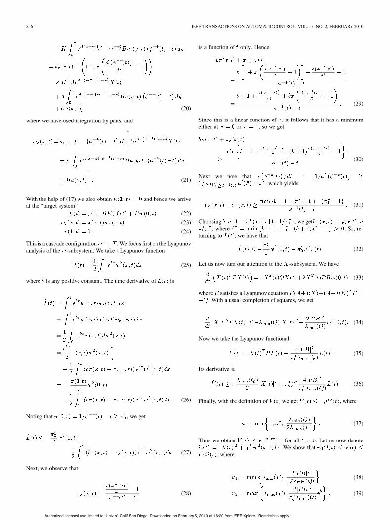
556 IEEE TRANSACTIONS ON AUTOMATIC CONTROL, VOL. 55, NO. 2, FEBRUARY 2010
(20)
where we have used integration by parts, and
(21)
With the help of (17) we also obtain and hence we arriveat the “target system”
(22)
(23)
(24)
This is a cascade configuration . We focus first on the Lyapunovanalysis of the -subsystem. We take a Lyapunov function
(25)
where is any positive constant. The time derivative of is
(26)
Noting that , we get
(27)
Next, we observe that
(28)
is a function of only. Hence
(29)
Since this is a linear function of , it follows that it has a minimumeither at or , so we get
(30)
Next we note that, which yields
(31)
Choosing , we get, where . So, re-
turning to , we have that
(32)
Let us now turn our attention to the -subsystem. We have
(33)
where satisfies a Lyapunov equation. With a usual completion of squares, we get
(34)
Now we take the Lyapunov functional
(35)
Its derivative is
(36)
Finally, with the definition of we get , where
(37)
Thus we obtain for all . Let us now denote. We show that
, where
(38)
(39)
Authorized licensed use limited to: Univ of Calif San Diego. Downloaded on February 5, 2010 at 16:20 from IEEE Xplore. Restrictions apply.

IEEE TRANSACTIONS ON AUTOMATIC CONTROL, VOL. 55, NO. 2, FEBRUARY 2010 557
It then follows that for all . Nowwe consider the norm . We recall thebackstepping transformation (19) and introduce its inverse
(40)
It can be show that and, where
(41)
(42)
(43)
(44)
and where and . Furthermore, we canshow that
(45)
(46)
(47)
(48)
With a few substitutions we obtain that ,where and . Fi-nally, we get , which com-pletes the proof of the theorem with and with .By choosing , i.e., by picking positiveand such that
(49)
we get , so is independent of .While Theorem 1 provides a stability result in terms of the system
norm , we would like to also get a stabilityresult in terms of the norm . Towards that end,we first observe that
(50)
(51)
With these identities and Theorem 1 we obtain the following.
Theorem 2: Consider the closed-loop system consisting of the plant(12)–(14) and the controller (17) and let Assumptions 1 and 2 hold.There exist positive constants and (the latter one being independentof ) such that
(52)
for all , where is as in the proof of Theorem 1 and
(53)
IV. OBSERVER DESIGN WITH TIME-VARYING SENSOR DELAY
We give a brief presentation of an observer design for an LTI systemswith a time-varying sensor delay:
(54)
(55)
We approach the observer design in a two-step manner:• Design an observer for the delay state since the output
is delayed.• Use a model-based predictor to advance the estimate of
by the delay time .We start by writing (54) as
. Then we introduce a state estimator foras ,where is selected so that the matrix is Hurwitz, i.e.,so that the system , where
, is exponentially stable in the timevariable . Let us now denote . This variable isgoverned by the differential equation
(56)
Now we take , which is an estimate of thepast state , and advance it by the delay time ,obtaining the estimate of the current state as
.To summarize, the observer is given by the equations
(57)
(58)
This observer has a structure that displays duality with respect to thepredictor-based controller (10) in two interesting ways:
• While controller (10) employs prediction over the future period, the observer (57)–(58) employs prediction over the
past period .• While controller (10) involves a time derivative of , the
observer (57)–(58) involves a time derivative of .In the case of a constant sensor delay, , the observer(57)–(58) reduces to [9], [12], [25].
V. EXAMPLES
The first two examples violate some of the assumptions of the theorybut are valuable in illustrating the design principle. The other two ex-amples fit the assumptions.
Example 5.1: (Linearly growing delay.) We consider ,which means that the delay time is linearly growing and is unbounded.
Authorized licensed use limited to: Univ of Calif San Diego. Downloaded on February 5, 2010 at 16:20 from IEEE Xplore. Restrictions apply.

558 IEEE TRANSACTIONS ON AUTOMATIC CONTROL, VOL. 55, NO. 2, FEBRUARY 2010
(In addition, the assumption that the delay is strictly positive for alltime is violated, but this assumption is less essential.) So, the predictorfeedback (10) assumes the form
(59)
It is interesting to observe that this system has zero dead time, sincethe initial delay is zero and the controller continues to compensate thedelay for . The control signal is and, since
, the control signal remains a bounded functionin spite of the delay growing unbounded.
This is potentially confusing as some difficulty should arise in a systemwhere the delay is growing unbounded. The difficulty manifests itselfwhen the system is subject to a disturbance or modeling error. In thatcase the control signal will not be given bybut will be governed by the feedback law (59). In this feedback lawthe gains grow exponentially with time. In the presence of a persistentdisturbance, which prevents from settling, the control signal willgrow unbounded as its gains grow unbounded.
Example 5.2: (Prediction time grows exponentially.) We consider. In this case
(60)The gain growth in is more pronounced than in Example 5.2—thegains grow as an exponential of an exponential.
Example 5.3: (Bounded delay with a constant limit.) We consider, where the prediction time is
The initial value of the prediction time is , the finalvalue is , and the uniform bound on the prediction timeis . Furthermore, the uniform bound on the quantity
is 1. Hencethe feedback law
employs bounded gains and achieves exponential stability (it alsoachieves a finite disturbance-to-state gain).
Example 5.4: (Bounded delay function without a limit.) In the pastthree examples the function was monotonic and it had a limit(in two of the three examples the function itself also had a limit).Now we consider an example where is oscillatory. Let
and denote . So, the gains of thepredictor feedback
(61)
Fig. 1. Linear system with time-varying actuatordelay .
Fig. 2. Oscillating delay function in Example 5.4. Solid: , dashed: .
are uniformly bounded. Now we consider a specific first-order example
(62)
namely, . In closed loop with the control law
where , the plant (62) has an explicit solution
.(63)
The explicit form of the control signal is(see Fig. 1). The explicit formulae
for both and require , which is given by .Figs. 2 and 3 show the graphs of the delay, state, and control functions.The gain is chosen as to achieve visual clarity about theLTV character of the overall system, particularly about the responseof , which has a “wavy” character to achieve compensation of theoscillating delay function.
Example 5.5: (Observer.) We illustrate the observer design (57),
(58) for a second order system with ,
, and . The resulting observer is(64)
(65)
(66)
(67)
VI. CONCLUSION
For predictor feedback for LTI systems with a time-varying delay,we have proved exponential stability under several conditions on thedelay function :
Authorized licensed use limited to: Univ of Calif San Diego. Downloaded on February 5, 2010 at 16:20 from IEEE Xplore. Restrictions apply.

IEEE TRANSACTIONS ON AUTOMATIC CONTROL, VOL. 55, NO. 2, FEBRUARY 2010 559
Fig. 3. State and control signal evolution for Example 5.4. The control “kicksin” at . The “waviness” in the control is for the purposeof compensation of the time-varying (oscillating) delay.
• the delay function is strictly positive (technical conditionwhich ensures that the state space of the input dynamics can bedefined);
• the delay function is uniformly bounded from above;• the delay rate function, , is strictly smaller than 1, i.e., the
delay may increase at a rate smaller than 1;• the delay rate function is uniformly bounded from below (by
a possibly negative finite constant), i.e., the delay may decrease ata uniformly bounded rate.
These four conditions need to be satisfied simultaneously but they arenot restrictive and they have two natural implications on the growth anddecrease of the delay. First, the delay can grow at a rate strictly smallerthan 1 but not indefinitely, because the delay must remain uniformlybounded. Second, the delay may decrease at any uniformly boundedrate but not indefinitely, because the delay must remain positive.
It may be somewhat disappointing, though inherent in the problem,that the delay function needs to be known sufficientlyfar in advance in order to be able to compute , which is neededin the controller (10). If the delay is bounded by , it is sufficient thatthe function be know seconds in advance. For instance, inExample 5.4 and in Fig. 2, . An approximate real-time com-putation of can be conducted using the differential equation
, where and . This idea isbased on the singular perturbation approach and will result in a stablemainainance of thanks to the boundary layer being ex-ponentially stable since .
A small error in the knowledge of can be tolerated (the errorneeds to be sufficiently small and sufficiently slow). This robustnessresult is provable due to the fact that the nominal closed-loop system
under predictor feedback is exponentially stable. The topology of thesystem in the robustness proof involves an norm of , ratherthan the norm.
Another approach to studying stability in the presence of delays is theinvariance principle [23, Theorem IV.4.2]. However, with the approachwe pursue, which involves a strict Lyapunov functional and explicitnorm estimates, we avoid a separate study of orbital precompactness[23, Theorem IV.5.2].
REFERENCES
[1] Z. Artstein, “Linear systems with delayed controls: A reduction,” IEEETrans. Autom. Control, vol. AC-27, no. 4, pp. 869–879, Aug. 1982.
[2] M. C. Delfour, “Linear quadratic optimal control problem with delaysin state and control variables: A state space approach,” SIAM J. ControlOptim., vol. 24, pp. 835–883, 1986.
[3] M. C. Delfour and J. Karrakchou, “State space theory of linear timeinvariant systems with delays in state, control and observation varia-blesPart II,” J. Math Anal. Appl., vol. 125, pt. II, pp. 400–450, 1987.
[4] Y. A. Fiagbedzi and A. E. Pearson, “Feedback stabilization of linear au-tonomous time lag systems,” IEEE Trans. Autom. Control, vol. AC-31,no. 9, pp. 847–855, Sep. 1986.
[5] K. Gu and S.-I. Niculescu, “Survey on recent results in the stability andcontrol of time-delay systems,” Trans. ASME, vol. 125, pp. 158–165,2003.
[6] K. Ito, “Regulator Problem for Hereditary Differential Systems withControl Delays,” NASA, ICASE Rep. 82-31, 1982.
[7] M. Jankovic, “Forwarding, backstepping, and finite spectrum assign-ment for time delay systems,” in Proc. Amer. Control Conf., 2006, pp.5618–5624.
[8] M. Jankovic, “Recursive predictor design for linear systems with timedelay,” in Proc. Amer. Control Conf., 2008, pp. 4904–4909.
[9] J. Klamka, “Observer for linear feedback control of systems with dis-tributed delays in controls and outputs,” Syst Control Lett., vol. 1, pp.326–331, 1982.
[10] M. Krstic, “Lyapunov tools for predictor feedbacks for delay systems:Inverse optimality and robustness to delay mismatch,” Automatica, vol.44, pp. 2930–2935, 2008.
[11] M. Krstic, “On compensating long actuator delays in nonlinear con-trol,” IEEE Trans. Autom. Control, vol. 53, no. 7, pp. 1684–1688, Aug.2008.
[12] M. Krstic and A. Smyshlyaev, “Backstepping boundary control for firstorder hyperbolic PDEs and application to systems with actuator andsensor delays,” Syst. Control Lett., vol. 57, pp. 750–758, 2008.
[13] W. H. Kwon and A. E. Pearson, “Feedback stabilization of linear sys-tems with delayed control,” IEEE Trans. Autom. Control, vol. AC-25,no. 2, pp. 266–269, Apr. 1980.
[14] A. Z. Manitius and A. W. Olbrot, “Finite spectrum assignment for sys-tems with delays,” IEEE Trans. Autom. Control, vol. AC-24, no. 4, pp.541–552, Aug. 1979.
[15] W. Michiels and S.-I. Niculescu, Stability and Stabilization of Time-Delay Systems: An Eignevalue-Based Approach. Singapore: SIAM,2007.
[16] S.-I. Niculescu, Delay Effects on Stability. New York: Springer, 2001.[17] S.-I. Niculescu and A. M. Annaswamy, “An adaptive Smith-controller
for time-delay systems with relative degree ,” Syst. ControlLett., vol. 49, pp. 347–358, 2003.
[18] M. Nihtila, “Adaptive control of a continuous-time system with time-varying input delay,” Syst. Control Lett., vol. 12, pp. 357–364, 1989.
[19] M. Nihtila, “Finite pole assignment for systems with time-varying inputdelays,” in Proc. IEEE Conf. Decision Control, 1991, pp. 927–928.
[20] J.-P. Richard, “Time-delay systems: An overview of recent advancesand open problems,” Automatica, vol. 39, pp. 1667–1694, 2003.
[21] G. Tadmor, “The standard problem in systems with a single inputdelay,” IEEE Trans. Autom. Control, vol. 45, no. 3, pp. 382–397, Mar.2000.
[22] R. B. Vinter and R. H. Kwong, “The infinite time quadratic controlfor linear systems with state and control delays: an evolution equationapproach,” SIAM J. Control Optim., vol. 19, pp. 139–153, 1981.
[23] J. A. Walker, Dynamical Systems and Evolution Equations: Theory andApplications. New York: Plenum, 1980.
[24] K. Watanabe, “Finite spectrum assignment and observer for multivari-able systems with commensurate delays,” IEEE Trans. Autom. Control,vol. 31, no. 6, pp. 543–550, Jun. 1996.
[25] K. Watanabe and M. Ito, “An observer for linear feedback control lawsof multivariable systems with multiple delays in controls and outputs,”Syst. Control Lett., vol. 1, pp. 54–59, 1981.
[26] Q.-C. Zhong, Robust Control of Time-Delay Systems. New York:Springer, 2006.
Authorized licensed use limited to: Univ of Calif San Diego. Downloaded on February 5, 2010 at 16:20 from IEEE Xplore. Restrictions apply.