M arket access, economic geography and comparative ...drd28/geo3.pdf · Journal of International Economics 59 (2003) 1–23 M arket access, economic geography and comparative advantage:

Journal of International Economics 59 (2003) 1–23www.elsevier.com/ locate/econbase

M arket access, economic geography and comparativeadvantage: an empirical test

*Donald R. Davis, David E. WeinsteinDepartment of Economics, Columbia University, 420 W. 118th St. MC 3308, New York, NY 10027,

USA

Received 25 October 1999; received in revised form 12 November 2001; accepted 10 December 2001

Abstract

Traditional neoclassical models of comparative advantage suggest that, all else equal, acountry with idiosyncratically strong demand for a good will be an importer of that good.However, there is a contrary tradition that emphasizes the advantages of a large homemarket as a foundation forexports of a good. One recent formalization of this home marketapproach falls within what is termed the new economic geography. This paper integratescore models of Heckscher–Ohlin and Krugman [American Economic Review 70 (1980)950] to investigate whether such home market effects matter empirically in manufacturingfor a set of OECD countries. The evidence suggests that home market effects are importantfor a broad segment of OECD manufacturing. 2002 Elsevier Science B.V. All rights reserved.

Keywords: Increasing returns; Economic geography; Comparative advantage

JEL classification: F1; D5; E1

1 . Market access, economic geography and comparative advantage: anempirical assessment

The empirical trade literature has focused strongly in recent years on under-standing determinants of the pattern of trade. In a seminal contribution, Leamer

*Corresponding author. Tel.:11-212-854-6880; fax:11-212-854-8059.E-mail address: [email protected](D.E. Weinstein).

0022-1996/02/$ – see front matter 2002 Elsevier Science B.V. All rights reserved.PI I : S0022-1996( 02 )00088-0

mailto:[email protected]

2 D.R. Davis, D.E. Weinstein / Journal of International Economics 59 (2003) 1–23

(1984) examines this question in a version of the Heckscher–Ohlin modelfeaturing factor price equalization (FPE) and equal numbers of goods and factors.Leamer identifies a set of twelve productive resources that correlate well withcountries’ net trade vectors. One limitation of Leamer’s approach is the focus onexplaining the net trade vector. The reason this is a limitation is that it is wellunderstood that the real intellectual capital of the theory is the predictions aboutthe cross-country pattern of production, which is then coupled with a rudimentaryand implausible theory positing identical structures of absorption.

Recognition of this limitation led researchers such as Harrigan (1995, 1997) andBernstein and Weinstein (2002) to focus directly on the model’s ability to predictcross country patterns of production. Within the framework of the frictionless FPEHeckscher–Ohlin model, this divorce between the patterns of production andabsorption makes perfect sense. However this makes less sense in a world inwhich trade frictions matter. And other contributions to the recent research agenda,including inter alia McCallum (1995) and Davis and Weinstein (1999) haveemphasized instead the importance of these frictions for understanding trade.

Trade frictions segment markets, giving rise to differences in price indicesacross locales. Moreover, these frictions imply that the geographical distribution ofdemand across markets will matter for local production patterns. In such a case,investigation of the pattern of production cannot proceed without attention tounderlying demand conditions. In order to investigate this empirically, one needsto commit to specific models. A fundamental divide may be identified betweentwo classes of models. In the first class, unusually strong demand for a good,ceteris paribus, makes a country an importer of a good. An example would be aconventional two-sector neoclassical model with strictly downward sloping importdemands. However, there is an alternative tradition within the trade literaturewhich emphasizes an important interaction between demand conditions andproduction opportunities in which the production response to local demandconditions is so powerful that strong local demand for a product leads a country toexport that product. When such conditions exist, the literature terms it a homemarket effect.

It is important to recognize that there are a variety of models which potentiallycould give rise to such home market effects. For example, the so-called biologicalmodel of trade posits that nationally-differentiated products arise in response topeculiarities in local demand (cf. Bhagwati, 1982; Feenstra, 1982), in turneffectively giving rise to Ricardian advantages that lead a country to export thatproduct. It is likewise important to recognize that the exact determinants of thehome market effect may well differ across models so that it will be important insubsequent work to consider alternative specifications of the home market effectthat correspond to the distinct underlying models.

This paper develops one approach to identifying empirically the existence ofhome market effects. The foundation for our approach is Krugman (1980) asextended by Weder (1995). The underlying model is Dixit–Stiglitz monopolistic

D.R. Davis, D.E. Weinstein / Journal of International Economics 59 (2003) 1–23 3

competition, with the novelty that the relative strength of demand for differentclasses of differentiated products leads production to rise more than one-for-one inresponse to idiosyncratic local demand. Building further on Krugman (1980) andHelpman (1981), we show how to place this model within a multi-sectorHeckscher–Ohlin framework to ready it for empirical estimation.

The present paper builds on earlier work in this vein, including Davis andWeinstein (1996, 1998). The most important alteration to our earlier analyticframework is a more careful approach to characterizing idiosyncratic local demandwhich takes fuller account of the geographical structure of absorption and theresulting opportunities this provides to producers considering location in thevarious countries. The results prove favorable to the hypothesis of the existenceand importance of home market effects.

In recent years, a number of papers have extended the approach developed hereof assessing economic geography by examining the relationship between demandand output. In particular, Trionfetti (2001a,b) demonstrates that home marketeffects need not always arise in increasing returns models and develops alternativetests. Head and Ries (2001) test for home market effects using firm level data.Finally, in a very interesting paper, Feenstra et al. (2001) demonstrate that homemarket effects can arise even in models in which all output is homogeneous.

2 . Theoretical framework for hypothesis testing

The broad outlines of our theoretical framework follow Davis and Weinstein(1996). The objective is to distinguish a world in which trade arises due toincreasing returns as opposed to comparative advantage. This is very difficult if wefocus on the class of zero transport cost increasing returns models deriving fromKrugman (1979) and Lancaster (1980). However this is possible if we focusinstead on the class of trade models that have come to be known as economicgeography, which interact increasing returns and trade costs in general equilib-rium.

We begin by sketching the model of Krugman (1980). The model is one ofmonopolistic competition. There are two classes of goods, each with manyvarieties. All varieties are symmetric in production and demand. Each variety isproduced under increasing returns to scale with a fixed cost and constant marginalcosts in units of labor. Preferences are the iso-elastic Dixit–Stiglitz form. Thenovelty in Krugman’s paper is the introduction to this framework of costs of tradein an iceberg form (for one unit of a good to arrive,t . 1 units must be shipped).He further assumes that there are two countries which are mirror images of eachother. They have the same labor forces. The difference lies in their demandstructure. For simplicity, he assumes that consumers come in two types, eachspecialized to consume all varieties of only one of the two classes of goods. Inaddition, he assumes that the sole difference between the countries is that one


country is predominantly populated by those who consume varieties of one of theclasses of goods, and vice versa (in perfect mirror fashion) for the other. Thesymmetry insures factor price equalization in spite of the trade costs.

An important feature of the model is that the combination of constant mark-upsand free entry implies that in equilibrium output per firm is the same acrossmarkets in spite of the trade costs. This means that a full description of theequilibrium can be given by the number of varieties of each of the two typesproduced in each country. Letm be the number of varieties of goodg produced atHome relative to those produced abroad. Let as , 1 be the ratio of demand for atypical import relative to a domestically produced variety in the same class. Letl

represent the ratio of demanders for goodg at Home relative to the number inForeign. Krugman shows that in the range of incomplete specialization, therelative production levelsm can be described as:

l2s]]m 5 12ls

When l51, demand patterns are identical and the countries produce the samenumber of varieties in each industry, leaving a zero net balance. This will play animportant role when we turn to our empirical implementation as it suggests thatpredictions of production structure, ceteris paribus, should be centered around aneven distribution of the industries across the countries. Idiosyncratic demandcomponents will then explain deviations from this neutral production structure.

Moreover, we need to consider closely the way in which idiosyncratic demandcomponents will translate into alterations in production structure. From above, andfor the range of incomplete specialization for which these relations are valid,

2≠m 12s] ]]]5 . 12≠l (12sl)

Krugman emphasized that this will imply that countries with a large home marketfor a good will be net exporters of that good. For our purposes it is convenient tofocus on an equivalent statement of this result that speaks directly to theimplications for production. That is, idiosyncratic demand patterns (indexed byl)have amagnified impact on production patterns. This will play a crucial role in ourempirical implementation, helping to separate the influences of economic geog-raphy from that of comparative advantage.

Why does the home market effect arise? In the presence of trade costs,producers will have an incentive to locate near the larger source of demand. This iscounterbalanced by the fact that as more and more producers leave the smallermarket, those who remain experience the trade costs not only as an inhibition ontheir deliveries to the larger market, but also as protection against the manyproducers who have located in that larger market. Ex ante it may not seem obviouswhich of these influences will dominate. However, it is possible to show that if theshare of varieties produced moved exactly one-for-one with the idiosyncratic


demand that those producers located in the large country would have higherdemand for their products than those located in the smaller market for that good.Since equilibrium requires that the derived demand be the same for all producers,this implies residual incentives for producers to move to the large market—hencethe home market effect.

It is likewise important to think about why the home market effect does notarise in the conventional constant returns to scale comparative advantage frame-work. The logic turns out to be very simple. Consider a positive shock to the homedemand structure for a good. Will this call forth additional local supply, and if sowill supply move more than one-for-one (as required for the home market effect)?If the production set is strictly convex, additional supply of the good will beforthcoming only if its relative price rises. But then, provided the foreign exportsupply curve has the conventional positive slope, this will also call forth additionalnet exports from abroad. In such a case, the idiosyncratic demand will be partlymet by additional local supply and partly by higher imports. Local supply, then,moves less than one-for-one with the idiosyncratic demand. In this conventionalcomparative advantage world, there is no home market effect.

Of course, Krugman (1980) cannot be taken straight to data. Such models ofeconomic geography contemplate highly abstract worlds in order to provide cleartheoretical insights. Even in such stark models, the inherent complexity of theproblems frequently defies analytic solution. While the robustness of the homemarket effect has been explored along a variety of dimensions (e.g. Weder, 1995),there is no single fully-solved model that has simultaneously incorporated themyriad elements essential for empirical implementation. Our approach is to hew asclosely as possible to the theory, and so provide a highly-structured interpretationof the models. Where it is not possible to provide a full solution, we make what weconsider the most sensible match between theory and specification.

3 . Implementing the search for home market effects

3 .1. Methodology

We begin with a sketch of the theoretical framework. The specification and datawork consider three levels of product aggregation: Varieties, Goods, and Indus-tries. Varieties play an important theoretical role within the model of economicgeography. In the Dixit and Stiglitz (1977) formulation, they are the locus ofincreasing returns in production, as well as the elements across which consumershave a preference for variety. While they play an important theoretical role, weassume they exist at a greater level of disaggregation than exists in our data.Goods, in our formulation, can be thought of in two ways. Under the hypothesis ofincreasing returns, a good is a collection of a large number of varieties producedunder monopolistic competition. It is at the goods level that differences in the


composition of demand give rise to home market effects. By contrast, under thehypothesis of comparative advantage, a good is a traditional homogeneouscommodity. Industries, in both frameworks, consist of a collection of goodsproduced using a common technology. In the comparative advantage framework,we interpret these as simple Leontief input coefficients. In the increasing returnsframework, we assume that both fixed and marginal costs of all varieties of allgoods within an industry use inputs in a fixed proportion. In our data work,industries and goods are typically 3- and 4-digit ISIC data respectively.

The null hypothesis that we consider is that comparative advantage determinesproduction and trade. The particular model of comparative advantage that weimplement is the so-called square Heckscher–Ohlin (HO) model, i.e. with equalnumbers of goods and factors (cf. Ethier, 1984). All countries share identicalLeontief technologies of production, which are linearly independent, so that thetechnology matrix is invertible. Letn be an index of industries,g of goods, andcof countries. Let it stand for the whole world, and ROW stand for the rest of theworld (excluding countryc). Let X andX be total output in industryn ofngc ngROW

goodg for countryc and the rest of the world respectively. LetV be the vector ofc

endowments of countryc. Let V be the inverse of the technology matrix, andVng

be the row corresponding to thegth good in industryn. Then our Heckscher–Ohlin model of goods production is given by:

X 5V V (1)ngc ng c

The alternative that we consider is what we term the Helpman–Krugmanspecification. It is inspired by Helpman’s (1981) integration of Heckscher–Ohlinwith a zero transport cost model of monopolistic competition. But in place of thelatter we substitute the Krugman (1980) model of economic geography.

Accordingly, we assume output structure is determined in two stages. Weassume the Heckscher–Ohlin model determines the broad industrial structure of a

¯country. Let V be the nth row of an inverse technology matrix for industryn

output, where the coefficients indicate average inputs at the equilibrium scale pervariety (which is constant within an industry). LetG be the number of products inn

industry n. Then output in industryn in country c is given by:Gn

¯X 5OX 5V V (2)nc ngc n cg51

While we assume endowments map perfectly to industry-level output, we alsoassume they tell us nothing about the composition of production across the goodswithin an industry. Since all varieties of all goods within an industry are assumedto use the same mix of factors, these may be thought of as a composite factor—ananalogue to the single factor ‘labor’ of Krugman (1980). Because of the Leontieftechnology assumption, resource constraints become industry-specific within acountry.


We may think of the determination of the output of the various goods within anindustry in two stages. Absent idiosyncratic elements of demand, each countryallocates its resources across the goods within a particular industry in the sameproportion as all other countries. This provides the country with a base level ofproduction for each good in an industry that we denote SHARE. The secondcomponent arises when there are idiosyncratic elements of demand across thegoods—what we term IDIODEM. These give rise to home market effects, here amore than one-for-one movement of production in response to idiosyncraticdemand.

In order to make this precise, we must distinguish between a country’s demandfor a good produced in many locations, which we denoteD , from the derivedngc

demand facing producers in a particular locale which forms the basis for the˜construction of IDIODEM, the latter of which we denoteD (and which isngc

discussed in more detail below). We may denote the correlate for the rest of the˜world as D . Because output and demand shares figure prominently in ourngROW

discussion, it is convenient to define some additional variables. Letg ;ngROW

X /X be the share of goodg industry n in the rest of the world (andngROW nROW˜ ˜ ˜which, of course, varies withc). Let d ;D /D be the share of goodg inngc ngc nc

industry n’s derived demand in countryc. With these definitions in hand, thespecification may be written in a general form as:

X 5a 1b SHARE 1b IDIODEM 1e (3)ngc ng 1 ngc 2 ngc ngc

where

˜ ˜SHARE ;g X , IDIODEM ; (d 2d )X .ngc ngROW nc ngc ngc ngROW nc

IDIODEM is our measure of the extent of idiosyncratic derived demand. Theterm in parentheses measures the extent to which the relative demand for a goodwithin an industry differs from that in the rest of the world. If all countries demandgoods in the same proportion, then IDIODEM is identically zero. When relativedemand for producers of a good in one country is higher (lower) than that in therest of the world, IDIODEM is positive (negative). Multiplying this term byXnc

gives IDIODEM the correct scale and units to include in the regression.If instead we believe that endowments may matter for the structure of 4-digit

production, then Davis and Weinstein (1996) show that an appropriate way ofnesting the models is as follows:

˜ ˜X 5a 1b g X 1b (d 2d )X 1V V 1e , or (4)ngc ng 1 ngROW nc 2 ngc ngROW nc ng c ngc

X 5a 1b SHARE 1b IDIODEM 1V V 1e (49)ngc ng 1 ngc 2 ngc ng c ngc

Within the set of models contemplated in this paper, this approach allows us touse the estimate ofb to distinguish three hypotheses. In a frictionless world2


(comparative advantage or increasing returns), the location of demand does notmatter for the pattern of production, so we would predictb 5 0. When there are2

frictions to trade, demand and production are correlated even in a world ofcomparative advantage, reaching exactly one-for-one when the frictions forceautarky. However production does not rise in a more than one-for-one manner.Accordingly, if we find b e(0, 1], we conclude that we are in a world of2

comparative advantage with transport costs. Finally, in the world of economicgeography, we do expect the more than one-for-one response, henceb . 1.2

Summarizing, the estimate ofb allows us to distinguish three hypotheses:2

b 50 Frictionless world (comparative advantage or IRS)2

b e(0, 1] Comparative advantage with frictions2

b .1 Economic geography2

These form the basis for our hypothesis tests.Direct estimation of Eq. (4) is not possible because of the simultaneity problem

arising from having industry output on the right-hand side and the output of a goodwithin that industry on the left. We can eliminate this simultaneity by rememberingthat, in our framework, endowments determine industry output. Using endowmentsas instruments forX eliminates the simultaneity problem.nc

There are a number of ways in which we can estimate Eq. (4) in addition toestimating the full system. If one believes that endowments do not matter at thegoods level, then one can forceV to equal zero for every factor and industry. Ifone excludes factor endowments, one should expect the coefficientb to equal1

unity. This is due to the fact that ceteris paribus one expects the share of goodsproduction within an industry to be the same across countries. While Davis andWeinstein (1996) confirm this, the parameter often has much larger standard errorsand deviates far from unity in specifications including endowments. This owes tothe high degree of multicollinearity between SHARE (which is formed in partusing endowment instruments) and the endowments. Since we found that thecrucial coefficient onb in specifications with endowments is largely invariant to2

the inclusion of SHARE, we dropped the latter from our specifications with1endowments.

1Davis and Weinstein (1996, 1999) found that in specifications with endowments and SHARE,b is1

negative and significant. This likely results from an identification problem that arises when we include˜SHARE and endowments. SinceX is a linear function of endowments, if there were no movement innc

g across countries, SHARE would be perfectly collinear with endowments and we could notngROW

estimate a coefficient. This is what would have occurred if we had calculated SHARE usinggngW

(where W indicates world values) instead ofg . The linear relationship between endowments andngROW

X̂ means that we would obtain an identical coefficient if we replaced SHARE with (g 2nc ngROWˆg )X . Identification here is achieved by examining the difference betweeng andg . This isngW nc ngROW ngW

likely to produce a negative coefficient because the share of four-digit output in the rest of the world islikely to be below the world average precisely when output in a country is above average.


Our construction of IDIODEM contrasts with the approach in the earlier Davisand Weinstein (1996) by focusing not only on locally idiosyncratic demand, butrather a derived demand that takes account of idiosyncracies in demand in

˜neighboring countries as well. Let this derived demand be denoted byD . This isngc

derived in a few steps. First we run industry-level gravity regressions to obtainparameters reflecting the impact of distance on demand. We then use theseelasticities to form weighted derived demands for each market subject to a scalingso that the sum of derived demands equals world demand for the entire market. Wefollow Leamer (1997) in our specification of the distance of a country from itself.These derived demands then serve as the input for calculations of IDIODEM. Ourestimates of the gravity equation are reasonable and the measures of IDIODEMdepart in sensible ways from the corresponding measures in Davis and Weinstein

2(1996).

3 .2. Data

The theories examined in this paper relate the structure of output to the structureof a country’s available factor endowments and idiosyncratic components ofdemand facing a country’s producers. This idiosyncratic demand, in turn, is aweighted average of absorption across a country’s trading partners. The weightsthemselves depend on estimates from a gravity equation of trade, hence oneconomic size, bilateral distance, and the characteristics of the particular industrywhich determine how demand dissipates with distance. These define the data

3required for our study.The OECD’s Compatible Trade and Production (COMTAP) data set is the

foundation for our study. It provides comparable trade and production data for 13members of the OECD disaggregated through the four-digit ISIC level [Australia,Belgium/Luxembourg, Canada, Finland, France, Germany, Italy, Japan, Nether-lands, Norway, Sweden, UK, USA] and for 22 members of the OECD through thethree-digit ISIC level [Austria, Denmark, Greece, Ireland, New Zealand, Portugal,Spain, Turkey, Yugoslavia]. National absorption is measured as the residualbetween output and net trade. World outputs and absorption levels are calculatedby summing across all available countries. Country capital stocks are from the

2A great deal more detail on our procedures is available in the working paper version of this paper,Davis and Weinstein (1999).

3In order to allow comparability with David and Weinstein (1996) we use the same data set, withone small amendment. For three sectors (other food products, rubber products, and professional andscientific equipment) Belgium–Luxembourg and Finland only report one four-digit sector within athree-digit sector. The values Belgium–Luxembourg and Finland report seem exceptionally large inthese sectors and lead us to suspect that data from other four digit sectors is included in these sectors.We therefore delete these industries from the data set. However, before doing so we re-ran ourequations with and without these sectors and found that the results in David and Weinstein (1996) arerobust to the inclusion of these three outliers.


Penn World Tables v. 5.6. World endowments of labor force by educational levelare from the UNESCOStatistical Yearbook. Fuel production is equal to the sum ofthe production of solid fuels, liquid fuels, and natural gas in coal-equivalent unitsas recorded in United Nations’Energy Statistics Yearbook. OECD’s COMTAPbilateral import and export numbers as prepared by Harrigan (1993) and madeavailable by Feenstra (1996) also underpin our gravity estimates. Country distanceis measured as the distance between the major economic centers in the respectivecountries and comes from Wei (1996). Measurements of how far countries arefrom themselves are taken from Leamer (1997).

Implementation of the economic geography framework, as embodied in Eq. (4),requires data at two levels of aggregation. At the higher level of aggregation,endowments determine the structure of output, while at the more disaggregatedlevel, economic geography is expected to exert its force. Unfortunately, theorydoes not indicate how to find a level of disaggregation where factor endowmentscease determining production structure and specialization is driven by increasingreturns and demand patterns. Our strategy is to use the most detailed cross-nationaldata we can find, and then assume that goods at the most disaggregated levelsrepresent a collection of monopolistically competitive varieties.

One concern about use of these data is whether the actual criterion for industrialclassification is congruent with the underlying theoretical categories. It is not.Actual classification is by product usage rather than simply by factor inputcomposition, as would be strictly required by the theory. Maskus (1991) examinedthis issue for ISIC three- and four-digit industries and found that while there isgreater similarity of factor intensities within three-digit sectors than across them,there still is substantial variation within three-digit sectors. Thus, although it istrue, for example, that the skilled to unskilled ratio in precision instrumentsexceeds that in textiles, there is no guarantee that this is true in comparing everygood produced within the respective industries. This could pose problems for ourtests. Within the economic geography framework, the assumption that all four-digitgoods in a three-digit industry use common input proportions served to replicatethe one-factor world of Krugman (1980). Heuristically this implied that ourproduction possibility surface had Ricardian flats, so a constant marginal oppor-tunity cost of shifting production from one good to another. Assuming instead thatthe goods use different input proportions could then imply a rising marginalopportunity cost of expanding one good in terms of the other. This might tend todiminish the responsiveness of production to idiosyncratic demand, implying thatthe IDIODEM coefficients might be less than unity even if the world is one ofeconomic geography. We acknowledge this possibility. Yet we remain skepticalthat this view is correct. Quite apart from the empirical issues of how the goodsare classified into industries, we know that if the number of goods is large relativeto the number of primary factors, the production surface (here in units of varieties)will again have flats [see Chipman (1992)]. Demand again could play the crucialrole in making the production and export patterns determinate—the key being that


production expansion for a single good again need not imply rising marginalopportunity cost in terms of other goods.

In principle, working at the four-digit level enabled us to break manufacturingup into 82 four-digit sectors, but because in 13 cases there is only one four-digitsector within a three digit sector, our sample is reduced to 69 four-digit and 27three-digit sectors. In addition, we dropped another 14 four-digit sectors due tomissing observations for some countries. In two sectors (fur dressing and dyeingand manufacturing goods, not elsewhere classified), we obtained large negativenumbers for domestic absorption for a number of countries so we dropped thoseindustries. For a few out of the remaining 702 observations, imputed domesticabsorption is negative but very small (1–2 per cent of production), and weattributed these negatives to measurement error and reclassified these amounts aszeros. There are 53 four-digit industries that we eventually used in the analysis.Many of the industries at the four-digit level, such as carpets and rugs, and motorvehicles, have been used as examples of monopolistically competitive industries.Indeed this level of disaggregation is basically the same as the one used byKrugman (1991) to support his hypothesis that geography matters for trade.

Because of data limitations, we are forced to measure domestic absorption as aresidual. Measuring domestic absorption by using a residual potentially introducesa bias into our sample through the mis-measurement of production. If productionis recorded at too high a level for a particular year, that will also tend to causemeasured absorption to rise. This creates a simultaneity problem if we usecontemporaneous demand. Furthermore, since the spirit of economic geographymodels is to explore how long-run historical demand deviations affect production,we thought it inappropriate to regress current production on current demand. Inorder to deal with both of these issues, we decided to use average demand over theperiod 1970–1975 to identify idiosyncratic components of demand, while othervariables in our regressions are values for 1985. We also ran all specifications withdemand calculated over the time period 1976–1985 and just 1985 and obtainedresults qualitatively the same.

4 . Estimation

4 .1. Pooling and aggregation

Our discussion makes a clear analytic distinction between various levels ofaggregation—varieties, goods, and industries. No such neat division exists in thedata. Thus the level of aggregation at which to implement our methodology is amatter of judgment and subject to data availability. If data were not a constraint,our inclination would be to think of goods as being at a level of disaggregationgreater than exists in the currently available data. Accordingly, in considering onlythis aspect of the problem, our preference is to work with the most disaggregated


data available. We do, though, consider a case at a higher level of aggregationsince this provides us with more observations and allows comparability withprevious work.

A second important consideration is the extent to which we should poolobservations across goods and industries. There is a clear advantage to pooling—itincreases the number of observations. This is potentially important, since in ourmost disaggregated runs we will have only thirteen observations per good.However there is correlatively an important disadvantage of pooling—it forces usto impose more structure on the estimates, and so leads us further from theunderlying analytic model. These include assumptions of common input pro-portions, demand symmetry, and equilibrium scale economies for all varieties ofall goods within an industry. Ex ante it is difficult to know whether we should behappier with estimates in which the theoretical model is more appropriate but thereare very few observations or the contrary case.

Our approach is to implement the estimation at a variety of levels of bothpooling and aggregation. If home market effects exist, we would at least like to seesome indication of their presence in the various exercises. However we shouldlikewise be cognizant that since these place quite distinct constraints on the data, itwill be asking too much to expect a perfect mapping among results from the variedruns.

We pursue four estimation exercises. In three of these, the dependent variable isfour-digit production, with the runs distinguished by the extent of pooling, whilethe fourth treats three-digit output as the dependent variable for individual industryruns. Consider first what we term the ‘pooled’ run. This exercise pools allfour-digit observations for the estimation of a single coefficient on IDIODEM. Thegreat advantage of this exercise is that there are 650 observations. The dis-advantages lie in that implicitly we must assume that either all industries arecomparative advantage or all are economic geography, and that we must assumethere is a common structure determining the coefficient on IDIODEM for all goodsin all industries. We next move to the opposite extreme, that of individual‘four-digit’ good runs. The advantages of this exercise are that it is closest to theanalytic structure we posit and that it allows the most detailed comparison acrosssectors of the presence or absence of home market effects. The disadvantage is thatdata availability implies there are only thirteen observations per four-digit sector.We next report an intermediate approach which pools all observations for four-digit goods within a three digit industry. We may term these ‘industry-pooled’runs. This approach trades off the advantages of the previous two exercises. Itimposes less structure than the fully pooled runs, but typically has four times asmany observations as the individual four-digit industry runs. This also suggests thedownside, namely the fact that it forces us to impose some common structurewithin industries that may not be fully suggested by the results in the four-digitruns themselves.

Our final exercise returns to individual sectoral runs. The departure is that


industries are now defined as two-digit output, and goods are three-digit output,and so are now the dependent variables. This has two important advantages. Thefirst is that we do gain some observations relative to the four-digit runs, sincetwenty-two countries report the three-digit data. The second is that this structureand level of aggregation can be directly compared with results of Davis andWeinstein (1999) on Japanese regional data. There are three disadvantages to thisexercise. The first is the loss of observations relative even to the industry-pooledruns. The second is that the additional observations relative to the four-digit runscome through the addition of countries that likely have lower quality data. Third,for related reasons, moving from the initial thirteen to twenty-two countries likelyleads to a greater violation in our assumption of a common economic structure forall countries.

These four exercises provide different windows on the home market effect. Aswe have seen, each exercise has advantages and drawbacks. Hence to judge theresults, we should not rely too heavily on any single exercise, but rather on theconjunction.

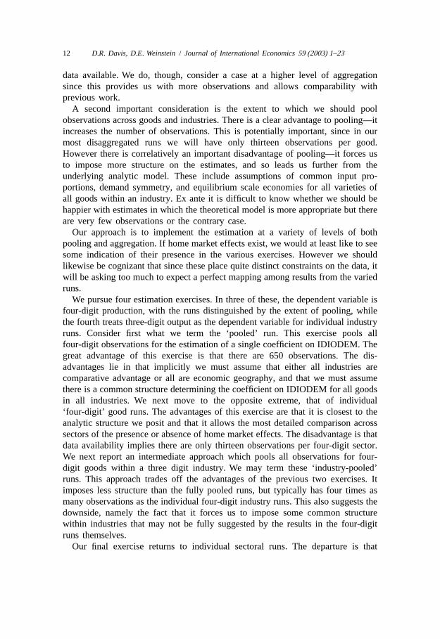
4 .2. A first view of the data

Before running regressions, we feel it is informative to present a picture of whatour data looks like. Eq. (3) is specified as a multivariate regression, so isimpossible to plot. However, if we constrain the coefficient on SHARE to equalunity, then simple algebraic manipulation enables us to rewrite Eq. (3) as

ang ˜ ˜ ˜]g 2g 5 1b (d 2d )1engc ngROW 2 ngc ngROW ngcXnc

If we plot the left-hand side of this equation against the term in parentheses, wecan obtain an approximate idea of how production distortions move with demanddistortions. What should we expect to see? In a frictionless comparative advantageworld, one would expect the two variables to be uncorrelated. Frictions in acomparative advantage world would produce a positive correlation, but the slopeof the line would be less than unity. Only in a world of home market effectsshould one see a positive correlation with a slope greater than unity.

We plot these in Fig. 1 for the four-digit sectors. The data clearly seems to bearrayed along a line with a slope that is greater than unity. Indeed, the fitted linehas a slope of 1.8, indicating that demand deviations typically produce more thanproportional production deviations.

4 .3. Pooled tests for the home market effect

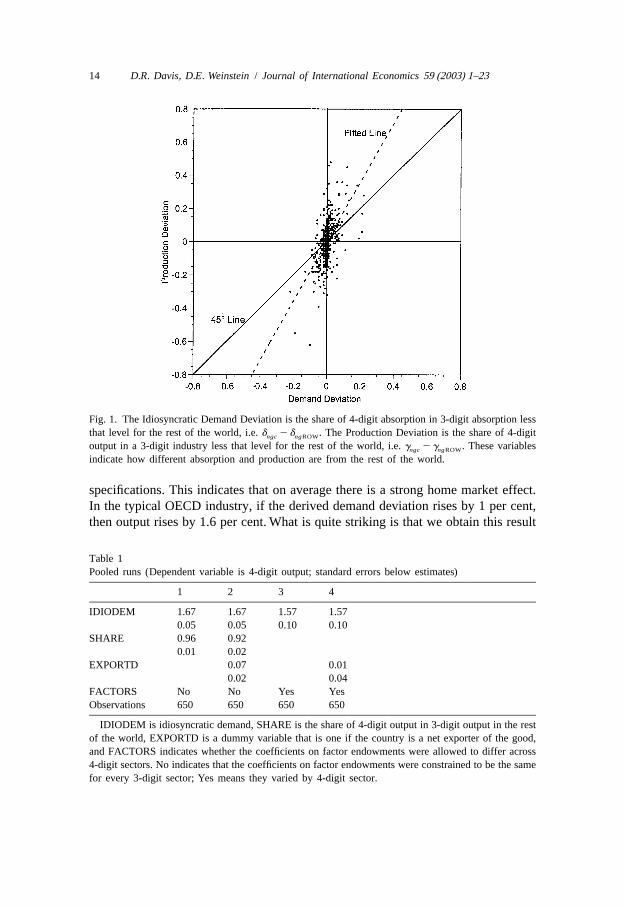
A more precise view of this relation comes from estimating Eq. (4) under avariety of specifications. The results from these pooled regressions appear in Table1. The most striking fact is that the coefficient on IDIODEM exceeds unity in all


Fig. 1. The Idiosyncratic Demand Deviation is the share of 4-digit absorption in 3-digit absorption lessthat level for the rest of the world, i.e.d 2d . The Production Deviation is the share of 4-digitngc ngROW

output in a 3-digit industry less that level for the rest of the world, i.e.g 2g . These variablesngc ngROW

indicate how different absorption and production are from the rest of the world.

specifications. This indicates that on average there is a strong home market effect.In the typical OECD industry, if the derived demand deviation rises by 1 per cent,then output rises by 1.6 per cent. What is quite striking is that we obtain this result

Table 1Pooled runs (Dependent variable is 4-digit output; standard errors below estimates)

1 2 3 4

IDIODEM 1.67 1.67 1.57 1.570.05 0.05 0.10 0.10

SHARE 0.96 0.920.01 0.02

EXPORTD 0.07 0.010.02 0.04

FACTORS No No Yes YesObservations 650 650 650 650

IDIODEM is idiosyncratic demand, SHARE is the share of 4-digit output in 3-digit output in the restof the world, EXPORTD is a dummy variable that is one if the country is a net exporter of the good,and FACTORS indicates whether the coefficients on factor endowments were allowed to differ across4-digit sectors. No indicates that the coefficients on factor endowments were constrained to be the samefor every 3-digit sector; Yes means they varied by 4-digit sector.


on the same data set used by Davis and Weinstein (1996). The crucial difference isthat the relevant idiosyncratic demand now accounts for the real geography of theOECD economies.

A final econometric issue that we must address is simultaneity. Is idiosyncraticdemand, as we posit, leading to a strong production response? Alternatively, is alevel of production beyond that our model explains drawing in its wakeidiosyncratic demand, creating only the appearance of home market effects? Theideal solution to this problem would be to find good instruments correlated withidiosyncratic demand, but not with output. Unfortunately we know of no suchgood instruments. Hence we cannot formally rule out the possibility thatsimultaneity influences our results. We can, though, take some steps to minimizeits potential influence. Moreover we can give some reasons, based on theconjunction of our studies, to suggest that this is very likely not an appealinginterpretation of our results.

First, we construct the demand variable based on an average of demands in thecountries ten to fifteen years prior to the estimation period. This removessimultaneity arising from contemporaneous correlations. Second, while we cannotinstrument for IDIODEM, we can control for some of the potential price effects inthe regression. In columns 2 and 4 we include a variable EXPORTD in ourspecification. EXPORTD is a dummy variable that equals one if the country is anet exporter of that commodity times the (instrumented) three digit output in thatsector. EXPORTD controls for the fact that countries that are net exporters tend tohave lower prices than countries that are net importers. As one can see thecoefficient on EXPORTD is positive as one should expect, but it hardly affects theoverall magnitude or significance of the coefficient on IDIODEM. The absence ofa strong impact of controlling for whether the country is a net exporter or notmakes it less likely that price movements associated with being a net exporter orimporter of a commodity are driving our results.

Finally, we need to think more closely about whether it is attractive to interpretour results as arising from simultaneity. The story would need to go something asfollows: While our model does a good job of predicting the pattern of production,it is surely less than perfect. Indeed, there could be some systematic influences onthe pattern of production left out, as for example Ricardian technical differencesacross countries. Hence a country or region may have a high level of production ofa good for reasons outside the model. In turn, this unusually high production maysuggest lower prices for the associated good, so lead idiosyncratic demand torespond to the production in a less than one-for-one manner. Thus the argumentwould be that by reversing the direction of true causality, we find home marketeffects of production responding more than one-for-one with idiosyncraticdemand.

The issue is whether this interpretation is attractive in light of the variousinvestigations we have pursued of the home market effect. It is straightforward toshow that under the hypothesis that production patterns are driven by comparative


advantage, plausible assumptions lead one to conclude that the potential upwardsimultaneity bias inb would diminish in the present paper relative to Davis and2

Weinstein (1996) because output is likely to have a much smaller effect on derived4demand than on local demand. Since the estimated coefficient in that paper was

0.3, this alone would suggest that simultaneity is not the likely cause of our findingof home market effects.

4 .4. The home market effect in industry runs

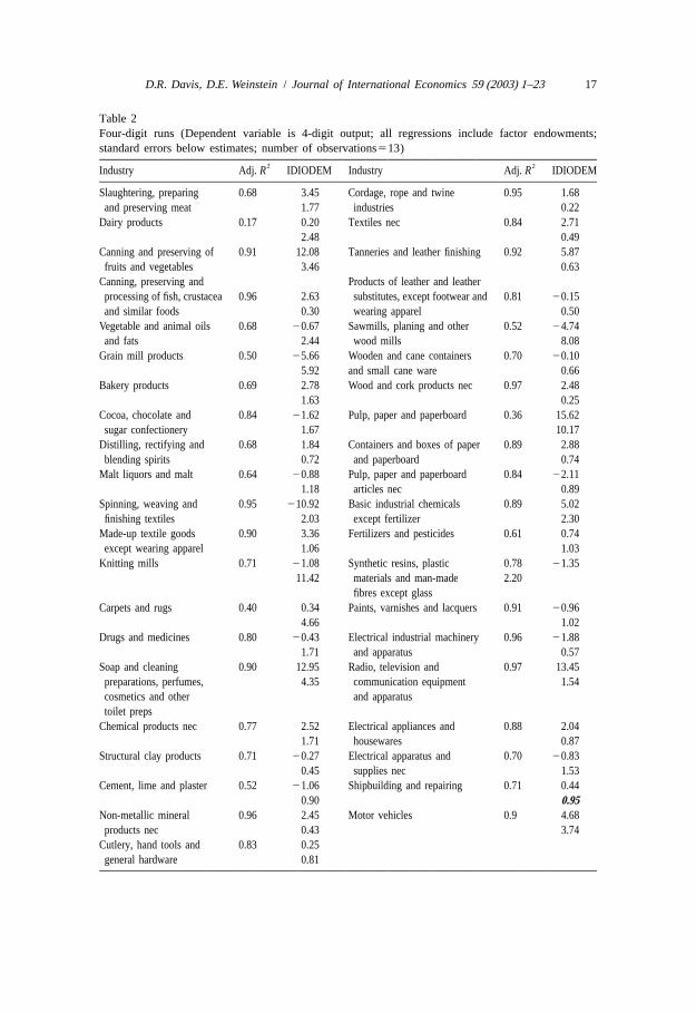
Having examined this by pooling all four-digit observations, we now move tothe opposite extreme, considering each four-digit sector on its own. The resultsappear in Table 2. Because there are very few degrees of freedom, it is quitedifficult to obtain statistical significance in these equations. Even so, we find thathalf of the sectors have coefficients on IDIODEM that are larger than unity and ofthese eleven are significantly greater than unity. By comparison, Davis andWeinstein (1996) only found half as many coefficients larger than unity and hardlyany that are significant. This suggests that in our data, some industries are constant

5and others increasing returns to scale. Home market effects are very much inevidence.

One way to increase the number of degrees of freedom relative to the four-digitruns is to conduct industry-pooled estimation. This pools the four-digit observa-tions within each three-digit industry, but allows the coefficient on IDIODEM tovary across three-digit industries. Relative to the fully-pooled runs, this allows usto relax the assumption that three-digit industries must either all be comparativeadvantage or all exhibit increasing returns. The results are presented in Table 3. Insimilar runs, Davis and Weinstein (1996) found that less than one-fifth of allsectors had point estimates above unity. Here, using our new measure of marketaccess, we now find that over half of the industries exhibit home market effects.Furthermore, while the earlier study found that none of the point estimates weresignificantly larger than unity, we now find that four of our coefficients have thisproperty. Moreover, while Davis and Weinstein (1996) rejected home market

4The story would specify an additional relation between idiosyncratic demand and production asfollows: IDIODEM 5vX 1h . For v [ (0, 1), it is straightforward to show that a sufficientngc ngc ngc

condition for the degree of bias to be increasing inv is that b ,1, i.e. that we are in a world of2

comparative advantage. The final step would be to note that the relevantv is likely to be lower in thepresent work than in Davis and Weinstein (1996), since local demand is plausibly more strongly relatedto local production than is a weighted average of local and rest-of-world demand.

5More subtle problems arise if individual industries themselves are composed of both IRS and CRSgoods. In alternative frameworks, Krugman (1980), Krugman and Venebles (1995) and Davis (1998)address this problem. The various contributions stress the potential role of absolute market size and thecross-good structure of trade costs in determining industrial structure. This remains an importantdirection for further empirical study.


Table 2Four-digit runs (Dependent variable is 4-digit output; all regressions include factor endowments;standard errors below estimates; number of observations513)

2 2Industry Adj.R IDIODEM Industry Adj. R IDIODEM

Slaughtering, preparing 0.68 3.45 Cordage, rope and twine 0.95 1.68and preserving meat 1.77 industries 0.22

Dairy products 0.17 0.20 Textiles nec 0.84 2.712.48 0.49

Canning and preserving of 0.91 12.08 Tanneries and leather finishing 0.92 5.87fruits and vegetables 3.46 0.63

Canning, preserving and Products of leather and leatherprocessing of fish, crustacea 0.96 2.63 substitutes, except footwear and 0.8120.15and similar foods 0.30 wearing apparel 0.50

Vegetable and animal oils 0.68 20.67 Sawmills, planing and other 0.52 24.74and fats 2.44 wood mills 8.08

Grain mill products 0.50 25.66 Wooden and cane containers 0.70 20.105.92 and small cane ware 0.66

Bakery products 0.69 2.78 Wood and cork products nec 0.97 2.481.63 0.25

Cocoa, chocolate and 0.84 21.62 Pulp, paper and paperboard 0.36 15.62sugar confectionery 1.67 10.17

Distilling, rectifying and 0.68 1.84 Containers and boxes of paper 0.89 2.88blending spirits 0.72 and paperboard 0.74

Malt liquors and malt 0.64 20.88 Pulp, paper and paperboard 0.84 22.111.18 articles nec 0.89

Spinning, weaving and 0.95 210.92 Basic industrial chemicals 0.89 5.02finishing textiles 2.03 except fertilizer 2.30

Made-up textile goods 0.90 3.36 Fertilizers and pesticides 0.61 0.74except wearing apparel 1.06 1.03

Knitting mills 0.71 21.08 Synthetic resins, plastic 0.78 21.3511.42 materials and man-made 2.20

fibres except glassCarpets and rugs 0.40 0.34 Paints, varnishes and lacquers 0.9120.96

4.66 1.02Drugs and medicines 0.80 20.43 Electrical industrial machinery 0.96 21.88

1.71 and apparatus 0.57Soap and cleaning 0.90 12.95 Radio, television and 0.97 13.45preparations, perfumes, 4.35 communication equipment 1.54cosmetics and other and apparatustoilet preps

Chemical products nec 0.77 2.52 Electrical appliances and 0.88 2.041.71 housewares 0.87

Structural clay products 0.71 20.27 Electrical apparatus and 0.70 20.830.45 supplies nec 1.53

Cement, lime and plaster 0.52 21.06 Shipbuilding and repairing 0.71 0.440.90 0.95

Non-metallic mineral 0.96 2.45 Motor vehicles 0.9 4.68products nec 0.43 3.74

Cutlery, hand tools and 0.83 0.25general hardware 0.81


Table 2. Continued2 2Industry Adj.R IDIODEM Industry Adj.R IDIODEM

Furniture and fixtures 0.90 1.50primarily of metal 0.82

Structural metal products 0.71 1.151.48

Fabricated metal products 0.92 4.03except machinery and 1.12equipment nec

Engines and turbines 0.94 20.630.44

Agriculture machinery 0.69 1.82and equipment 0.96

Metal and wood working 0.93 1.23machinery 1.25

Special industrial machinery 0.88 0.13and equipment except metal 2.05and wood workingmachinery

Office, computing and 0.77 27.49accounting machinery 4.36

Machinery and equipment, 0.85 3.81except electrical nec 1.48

effects in two-thirds of the three-digit sectors, we now reject economic geographyonly in two sectors, other chemicals and non-electrical machinery.

One word of caution is in order. Looking at the sectors, it is somewhatdisappointing that sectors like electrical machinery and transportation equipmentdo not have point estimates that exceed unity. A likely explanation is imprecisionof the estimates. In both of these sectors, the standard errors are so large that wecannot reject home market effects. Indeed the four-digit runs presented in Table 2indicate that in half the sectors within these industries (radio, television andcommunication equipment, electrical appliances and housewares, and motorvehicles), we do obtain point estimates for IDIODEM that exceed one.

Hence we conclude that, these problems notwithstanding, relative to previouswork these results do represent a striking degree of support for the economicgeography paradigm. Most sectors exhibit home market effects. Those that do notexhibit such effects typically have point estimates that are measured imprecisely.

It is useful to compare these results to those in our companion study onJapanese regional data. There we also found significant home market effects.Unfortunately, it is difficult to match our new results with those of Davis andWeinstein (1999) because that paper used Japanese data at a different level ofaggregation. However, if we aggregate the data so that we assume industries aredefined at the two-digit ISIC and goods at the three-digit ISIC, then we have aroughly comparable level of aggregation.

There are several issues to bear in mind about increasing the level of


Table 3Industry-pooled estimation (Dependent variable is 4-digit output; coefficients on factor endowmentsvary at the 4-digit level; standard errors below estimates)

Industry IDIODEM Obs.

Food products 2.51 1040.28

Beverage industries 1.11 260.61

Textiles 1.79 780.20

Leather 2.17 260.39

Wood products 2.16 390.23

Paper and pulp 0.89 390.57

Industrial chems. 1.02 390.86

Other chemicals 0.28 520.77

Other non-metallic 0.91 39mineral product

0.30Fabricated metals 1.49 52

0.48Machinery, except 0.11 78electric 0.36

Electrical mach. 0.42 520.44

Transportation equip. 0.69 260.92

aggregation. Because more countries report three-digit production data than four-digit, we have more degrees of freedom than on the four-digit runs. But the higherlevel of aggregation means that we increase the chance that we are pooling sectorsthat differ in many respects, including factor intensity. This may interfere with theoperation of home market effects. For example, while it is plausible that highdemand for motor vehicles might cause specialization in motor vehicles asopposed to motorcycles, it is less plausible that countries with high demand fortransport equipment are less likely to produce precision instruments. On Japanesedata, where we had compatible technology matrices, we could circumvent thisproblem by aggregating according to technological similarity, but on internationaldata, this is not possible. Furthermore, we are faced with the problem that thevariance in demand deviations shrinks at higher levels of aggregation. When wemove from four- to three-digit data, the variance in our demand deviation variablefalls by a factor of two for the countries for which we have comparable numbers.By comparison, Japanese regions had a demand deviation variance that was


comparable to international four-digit data. Finally the inclusion of countries likeTurkey and Yugoslavia in the three-digit sample probably exacerbates problemssuch as measurement error.

These reasons may help explain why Davis and Weinstein (1996) found asmaller impact of demand deviations on production deviations on more aggregateddata. Nevertheless, since we did find evidence of home market effects at a higherlevel of aggregation on Japanese data (albeit with more than twice the number ofdegrees of freedom), it may be useful to compare those results with ourinternational results at a higher level of aggregation.

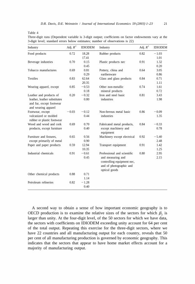
We present the results from goods-level estimation at the three-digit level inTable 4. Although only one sector, textiles, exhibits a coefficient on IDIODEMthat is significantly larger than unity, 9 out of our 26 sectors have point estimatesin excess of unity. By comparison, in Davis and Weinstein (1999), 9 out of 19sectors had point estimates larger than unity and 8 out of these 9 were significant.No doubt many of the reasons that we have highlighted above explain the relativeimprecision of our international results. Even so, there is a fair amount of overlapbetween the two sets of results. If we restrict attention to the 14 sectors that appearin both the international and regional data sets, we find that seven have coefficientson IDIODEM that are significantly larger than unity in the Japanese data and fivehave point estimates larger than unity in the international data. Interestingly, fourof the five international sectors that come up as having home market effects—textiles, iron and steel, transportation equipment, and precision instruments—areamong the seven sectors that also have measurable home market effects in theJapanese data. Although the large standard errors in these industry runs make itdifficult to make strong statements, there is a striking degree of overlap.Furthermore, the fact that these sectors have often been presented as canonicalexamples of economic geography by Krugman (1991) and others bolsters theplausibility of our point estimates.

Returning to our individual four-digit sector runs, we next examine the issue ofeconomic significance. Here we considerb-coefficients, which indicate how mucha one standard deviation movement in the independent variable moves thedependent variable. Over all, our estimates for the pooled specification indicatethat a one-standard-deviation movement in idiosyncratic demand moves pro-duction by about 0.15 standard deviations. While quite modest, it is still threetimes larger than the estimate in Davis and Weinstein (1996). However, since weare probably dealing with a mix of sectors, only some of which are monopolistical-ly competitive, it makes sense to calculate these coefficients on a sector-by-sectorbasis.

If one inspects theb-coefficients (reported in Davis and Weinstein, 1998) inmany sectors the home market effect is extremely important. For example inelectrical machinery sectors, we obtainb-coefficients that are typically in the 0.9range—indicating that the absorption linkage to production is very important.Overall, in the sectors where we detect coefficients on idiosyncratic demand thatare larger than unity,b-coefficients are typically around 0.5.


Table 4Three-digit runs (Dependent variable is 3-digit output; coefficients on factor endowments vary at the3-digit level; standard errors below estimates; number of observations is 22)

2 2Industry Adj.R IDIODEM Industry Adj. R IDIODEM

Food products 0.72 18.28 Rubber products 0.82 21.0317.41 1.01

Beverage industries 0.70 0.15 Plastic products nec 0.91 1.320.45 0.20

Tobacco manufactures 0.69 0.81 Pottery, china and 0.64 3.050.29 earthenware 0.86

Textiles 0.83 62.64 Glass and glass products 0.84 0.7120.35 1.11

Wearing apparel, except 0.85 20.53 Other non-metallic 0.74 1.610.18 mineral products 0.72

Leather and products of 0.20 20.32 Iron and steel basic 0.81 3.43leather, leather substitutes 0.80 industries 1.98and fur, except footwearand wearing apparel

Footwear, except 20.03 20.12 Non-ferrous metal basic 0.86 20.09vulcanized or molded 0.44 industries 1.35rubber or plastic footwear

Wood and wood and cork 0.69 0.70 Fabricated metal products, 0.84 20.33products, except furniture 0.40 except machinery and 0.78

equipmentFurniture and fixtures, 0.65 0.56 Machinery except electrical 0.92 25.40except primarily of metal 0.90 2.48

Paper and paper products 0.59 12.94 Transport equipment 0.91 1.4210.35 1.25

Industrial chemicals 0.91 20.61 Professional and scientific 0.80 2.950.45 and measuring and 2.15

controlling equipment nec,and of photographic andoptical goods

Other chemical products 0.88 0.711.14

Petroleum refineries 0.82 21.280.40

A second way to obtain a sense of how important economic geography is toOECD production is to examine the relative sizes of the sectors for whichb is2

larger than unity. At the four-digit level, of the 50 sectors for which we have data,the sectors with coefficients on IDIODEM exceeding unity account for 64 per centof the total output. Repeating this exercise for the three-digit sectors, where wehave 22 countries and all manufacturing output for each country, reveals that 50per cent of all manufacturing production is governed by economic geography. Thisindicates that the sectors that appear to have home market effects account for amajority of manufacturing output.


5 . Conclusion

This paper has examined data for a set of OECD countries to investigate theexistence of home market effects from idiosyncratic demand on the pattern ofproduction. We developed a framework that nests a conventional Heckscher–Ohlinframework (based on comparative advantage) with a model of economic geog-raphy. Within the context of these models, the simple comparative advantagemodel would not predict home market effects, while that of economic geographywould predict such effects.

The results provide support for the economic geography hypothesis of theexistence of home market effects. Within the context of the three modelsconsidered in this study, they also provide important evidence on the role andimportance of increasing returns in determining production structure for theOECD. A parallel investigation of 40 Japanese regions in Davis and Weinstein(1999) also finds such home market effects.

The broad picture that emerges draws on insights from Helpman (1981) andKrugman (1980). Within the context of the models considered, comparativeadvantage matters both in affecting the broad and fine industrial structure. Even atthe four-digit level, from one-third to one-half of OECD manufacturing outputseem to be governed by simple comparative advantage. However increasingreturns also play a vital role, in the particular form known as economic geography.These have measurable effects on production structure for as much as one-half totwo-thirds of OECD manufacturing output. Finally, we saw that the key toidentifying these effects is to introduce more geographical realism into our modelsof production and trade.

A cknowledgements

We are grateful to Tony Venables for very helpful suggestions.

R eferences

Bernstein, J., Weinstein, D.E., 2002. Do endowments predict the location of production? Journal ofInternational Economics 56 (1), 55–76.

Bhagwati, J.N., 1982. Shifting comparative advantage, protectionist demands, and policy response. In:Bhagwati, J.N. (Ed.), Import Competition and Response. University of Chicago.

Chipman, J.S., 1992. Intra-industry trade, factor proportions and aggregation. In: Rader, T.J. (Ed.),Economic Theory and International Trade: Essays in Memoriam. Springer-Verlag, New York.

Davis, D.R., 1998. The home market, trade, and industrial structure. American Economic ReviewDecember.

Davis, D.R., Weinstein D.E., 1996. Does economic geography matter for international specialization?Mimeo, National Bureau of Economic Research Working Paper[ 5706, August.

Davis, D.R., Weinstein, D.E., 1998. Market access, economic geography and comparative advantage: anempirical assessment. National Bureau of Economic Research Working Paper[ 6787, November.


Davis, D.R., Weinstein, D.E., 1999. Economic geography and regional production structure: anempirical investigation. European Economic Review February.

Dixit, A.K., Stiglitz, J.E., 1977. Monopolistic competition and optimum product diversity. AmericanEconomic Review 67 (3), 297–308.

Ethier, W.J., 1984. Higher dimensional issues in trade theory. In: Jones, R.W., Kenen, P.B. (Eds.).Handbook of International Economics, Vol. 1. North-Holland, New York.

Feenstra, R.C., 1982. Appendix. Product creation and trade patterns: a theoretical note on the‘biological’ model of trade in similar products. In: Bhagwati, J.N. (Ed.), Import Competition andResponse. University of Chicago.

Feenstra, R.C., 1996. U.S. imports, 1972–1994: data and concordances. National Bureau of EconomicResearch[5515, and National Bureau of Economic Research Trade Database, Disk 1.

Feenstra, R.C., Markusen, J.R., Rose, A.K., 2001. Using the gravity equation to differentiate amongalternative theories of trade. Canadian Journal of Economics 34 (2), 430–447.

Harrigan, J., 1993. OECD imports and trade barriers in 1983. Journal of International Economics.Harrigan, J., 1995. Factor endowments and the international location of production: econometric

evidence from the OECD, 1970–1985. Journal of International Economics.Harrigan, J., 1997. Technology, factor supplies and international specialization: testing the neoclassical

model. American Economic Review 87, 475–494.Head, K., Ries, J., 2001. Increasing returns versus national product differentiation as an explanation for

the pattern of US–Canada trade. American Economic Review 91 (4), 858–879.Helpman, E., 1981. International trade in the presence of product differentiation, economies of scale

and monopolistic competition: a Chamberlin–Heckscher–Ohlin approach. Journal of InternationalEconomics 11 (3).

Krugman, P.R., 1979. Increasing returns, monopolistic competition, and international trade. Journal ofInternational Economics 9 (4), 469–479.

Krugman, P.R., 1980. Scale economies, product differentiation, and the pattern of trade. AmericanEconomic Review 70, 950–959.

Krugman, P.R., 1991. Geography and Trade. Massachusetts Institute of Technology, Cambridge.Krugman, P.R., Venables, A.J., 1995. Globalization and the inequality of nations. Quarterly Journal of

Economics 110 (4), 857–880.Lancaster, K., 1980. Intra-industry trade under perfect monopolistic competition. Journal of Internation-

al Economics 10 (2), 151–175.Leamer, E., 1984. Sources of International Comparative Advantage. Massachusetts Institute of

Technology, Cambridge.Leamer, E., 1997. Access to western markets and eastern effort. In: Zecchini, S. (Ed.), Lessons from

the Economic Transition, Central and Eastern Europe in the 1990s. Kluwer Academic Publishers,Dordrecht, pp. 503–526.

Maskus, K.E., 1991. Comparing international trade data and product and national characteristics datafor the analysis of trade models. International Economic Transactions: Issues in Measurement andEmpirical Research, 17–56.

McCallum, J., 1995. National borders matter: Canada–US regional trade patterns. American EconomicReview 85 (3).

Trionfetti, F., 2001a. Public procurement, economic integration, and income inequality. The Review ofInternational Economics 9 (1), 29–41.

Trionfetti, F., 2001b. Using home-biased demand to test for trade theories. Weltwirtschaftliches Archiv137 (3), 404–426.

Weder, R., 1995. Linking absolute and comparative advantage to intra-industry trade theory. Review ofInternational Economics 3 (3).

Wei, S.J., 1996. Intra-national versus international trade: how stubborn are nations in globalintegration? National Bureau of Economic Research Working Paper[5531.

Documents

M arket access, economic geography and comparative ...drd28/geo3.pdf · Journal of International Economics 59 (2003) 1–23 M arket access, economic geography and comparative advantage: