Embed Size (px)
Citation preview
Rend. Sem. Mat. Univ. Pol. TorinoVol. 56, 4 (1998)
M. Bardi ∗ – S. Bottacin
ON THE DIRICHLET PROBLEM
FOR NONLINEAR DEGENERATE ELLIPTIC EQUATIONS
AND APPLICATIONS TO OPTIMAL CONTROL
Abstract.We construct a generalized viscosity solution of the Dirichlet problem for fully
nonlinear degenerate elliptic equations in general domains by the Perron-Wiener-Brelot method. The result is designed for the Hamilton-Jacobi-Bellman-Isaacsequations of time-optimal stochastic control and differential games with discon-tinuous value function. We study several properties of the generalized solution, inparticular its approximation via vanishing viscosity and regularization of the do-main. The connection with optimal control is proved for a deterministic minimum-time problem and for the problem of maximizing the expected escape time of adegenerate diffusion process from an open set.
Introduction
The theory of viscosity solutions provides a general framework for studying the partial differ-ential equations arising in the Dynamic Programming approach to deterministic and stochasticoptimal control problems and differential games. This theory is designed for scalar fully nonlin-ear PDEs
F(x, u(x), Du(x), D2u(x)) = 0 in �,(1)
where� is a general open subset of�N , with the monotonicity property
F(x, r, p, X) ≤ F(x, s, p, Y)
if r ≤ s andX − Y is positive semidefinite,(2)
so it includes 1st order Hamilton-Jacobi equations and 2nd order PDEs that are degenerateelliptic or parabolic in a very general sense [18, 5].
The Hamilton-Jacobi-Bellman (briefly, HJB) equations in the theory of optimal control ofdiffusion processes are of the form
supα∈A
�αu = 0 ,(3)
∗* Partially supported by M.U.R.S.T., projects “Problemi nonlineari nell’analisi e nelle applicazionifisiche, chimiche e biologiche” and “Analisi e controllo di equazioni di evoluzione deterministiche e stocas-tiche”, and by the European Community, TMR Network “Viscosity solutions and their applications”.
13
14 M. Bardi – S. Bottacin
whereα is the control variable and, for eachα,�α is a linear nondivergence form operator
�αu := −aαi j
∂2u
∂xi ∂x j+ bα
i∂u
∂xi+ cαu − f α,(4)
where f andc are the running cost and the discount rate in the cost functional, b is the drift ofthe system,a = 1
2σσ T andσ is the variance of the noise affecting the system (see Section 3.2).These equations satisfy (2) if and only if
aαi j (x)ξi ξ j ≥ 0 andcα(x) ≥ 0, for all x ∈ �, α ∈ A, ξ ∈ �N ,(5)
and these conditions are automatically satisfied by operators coming from control theory. In thecase of deterministic systems we haveaα
i j ≡ 0 and the PDE is of 1st order. In the theory oftwo-person zero-sum deterministic and stochastic differential games the Isaacs’ equation has theform
supα∈A
infβ∈B
�α,βu = 0 ,(6)
whereβ is the control of the second player and�α,β are linear operators of the form (4) and
satisfying assumptions such as (5).
For many different problems it was proved that the value function is the unique continuousviscosity solution satisfying appropriate boundary conditions, see the books [22, 8, 4, 5] and thereferences therein. This has a number of useful consequences, because we have PDE methodsavailable to tackle several problems, such as the numericalcalculation of the value function,the synthesis of approximate optimal feedback controls, asymptotic problems (vanishing noise,penalization, risk-sensitive control, ergodic problems,singular perturbations. . . ). However, thetheory is considerably less general for problems withdiscontinuousvalue function, because itis restricted to deterministic systems with a single controller, where the HJB equation is of firstorder with convex Hamiltonian in thep variables. The pioneering papers on this issue are dueto Barles and Perthame [10] and Barron and Jensen [11], who use different definitions of non-continuous viscosity solutions, see also [27, 28, 7, 39, 14], the surveys and comparisons of thedifferent approaches in the books [8, 4, 5], and the references therein.
For cost functionals involving the exit time of the state from the set�, the value functionis discontinuous if the noise vanishes near some part of the boundary and there is not enoughcontrollability of the drift; other possible sources of discontinuities are the lack of smoothnessof ∂�, even for nondegenerate noise, and the discontinuity or incompatibility of the boundarydata, even if the drift is controllable (see [8, 4, 5] for examples). For these functionals the valueshould be the solution of the Dirichlet problem
{
F(x, u, Du, D2u) = 0 in � ,
u = g on ∂� ,(7)
whereg(x) is the cost of exiting� at x and we assumeg ∈ C(∂�). For 2nd order equations, or1st order equations with nonconvex Hamiltonian, there are no local definitions of weak solutionand weak boundary conditions that ensure existence and uniqueness of a possibly discontinuoussolution. However a global definition of generalized solution of (7) can be given by the followingvariant of the classical Perron-Wiener-Brelot method in potential theory. We define
�:= {w ∈ BU SC(�) subsolution of (1), w ≤ g on∂�}
�:= {W ∈ BL SC(�) supersolution of (1), W ≥ g on ∂�} ,
On the Dirichelet problem 15
where BU SC(�) (respectively,BL SC(�)) denote the sets of bounded upper (respectively,lower) semicontinuous functions on�, and we say thatu : � → �
is a generalized solution of(7) if
u(x) = supw∈�
w(x) = infW∈�
W(x) .(8)
With respect to the classical Wiener’s definition of generalized solution of the Dirichlet problemfor the Lapalce equation in general nonsmooth domains [45] (see also [16, 26]), we only replacesub- and superharmonic functions with viscosity sub- and supersolutions. In the classical theorythe inequality supw∈� w ≤ infW∈� W comes from the maximum principle, here it comes fromtheComparison Principlefor viscosity sub- and supersolutions; this important result holds undersome additional assumptions that are very reasonable for the HJB equations of control theory, seeSection 1.1; for this topic we refer to Jensen [29] and Crandall, Ishii and Lions [18]. The maindifference with the classical theory is that the PWB solution for the Laplace equation is harmonicin � and can be discontinuous only at boundary points where∂� is very irregular, whereas hereu can be discontinuous also in the interior and even if the boundary is smooth: this is becausethe very degenerate ellipticity (2) neither implies regularizing effects, nor it guarantees that theboundary data are attained continuously. Note that if a continuous viscosity solution of (7) existsit coincides withu, and both the sup and the inf in (8) are attained.
Perron’s method was extended to viscosity solutions by Ishii [27] (see Theorem 1), whoused it to prove general existence results of continuous solutions. The PWB generalized solutionof (7) of the form (8) was studied indipendently by the authors and Capuzzo-Dolcetta [4, 1] andby M. Ramaswamy and S. Ramaswamy [38] for some special cases of equations of the form (1),(2). In [4] this notion is calledenvelope solutionand several properties are studied, in particularthe equivalence with the generalized minimax solution of Subbotin [41, 42] and the connectionwith deterministic optimal control. The connection with pursuit-evasion games can be found in[41, 42] within the Krasovskii-Subbotin theory, and in our paper with Falcone [3] for the Flemingvalue; in [3] we also study the convergence of a numerical scheme.
The purposes of this paper are to extend the existence and basic properties of the PWBsolution in [4, 1, 38] to more general operators, to prove some new continuity properties withrespect to the data, in particular for the vanishing viscosity method and for approximations ofthe domain, and finally to show a connection with stochastic optimal control. For the sake ofcompleteness we give all the proofs even if some of them follow the same argument as in thequoted references.
Let us now describe the contents of the paper in some detail. In Subsection 1.1 we recallsome known definitions and results. In Subsection 1.2 we prove the existence theorem underan assumption on the boundary datag that is reminiscent of the compatibility conditions inthe theory of 1st order Hamilton-Jacobi equations [34, 4]; this condition implies that the PWBsolution is either the minimal supersolution or the maximalsubsolution (i.e., either the inf orthe sup in (8) is attained), and it is verified in time-optimalcontrol problems. We recall that theclassical Wiener Theorem asserts that for the Laplace equation any continuous boundary functiong is resolutive(i.e., the PWB solution of the corresponding Dirichlet problem exists), and thiswas extended to some quasilinear nonuniformly elliptic equations, see the book of Heinonen,Kilpelainen and Martio [25]. We do not know at the moment if this result can be extended tosome class of fully nonlinear degenerate equations; however we prove in Subsection 2.1 that theset of resolutive boundary functions in our context is closed under uniform convergence as in theclassical case (cfr. [26, 38]).
In Subsection 1.3 we show that the PWB solution is consistentwith the notions of general-ized solution by Subbotin [41, 42] and Ishii [27], and it satisfies the Dirichlet boundary condition
16 M. Bardi – S. Bottacin
in the weak viscosity sense [10, 28, 18, 8, 4]. Subsection 2.1is devoted to the stability of thePWB solution with respect to the uniform convergence of the boundary data and the operatorF .In Subsection 2.2 we consider merely local uniform perturbations of F , such as the vanishingviscosity, and prove a kind of stability provided the set� is simultaneously approximated fromthe interior.
In Subsection 2.3 we prove that for a nested sequence of open subsets�n of � such that⋃
n �n = �, if un is the PWB solution of the Dirichlet problem in�n, the solutionu of (7)satisfies
u(x) = limn
un(x) , x ∈ � .(9)
This allows to approximateu with more regular solutionsun when∂� is not smooth and�n arechosen with smooth boundary. This approximation proceduregoes back to Wiener [44] again,and it is standard in elliptic theory for nonsmooth domains where (9) is often used todefinea generalized solution of (7), see e.g. [30, 23, 12, 33]. In Subsection 2.3 we characterize theboundary points where the data are attained continuously interms of the existence of suitablelocal barriers.
The last section is devoted to two applications of the previous theory to optimal control. Thefirst (Subsection 3.1) is the classical minimum time problemfor deterministic nonlinear systemswith a closed target. In this case the lower semicontinuous envelope of the value function is thePWB solution of the homogeneous Dirichlet problem for the Bellman equation. The proof wegive here is different from the one in [7, 4] and simpler. The second application (Subsection 3.2)is about the problem of maximizing the expected discounted time that a controlled degeneratediffusion process spends in�. Here we prove that the value function itself is the PWB solutionof the appropriate problem. In both casesg ≡ 0 is a subsolution of the Dirichlet problem, whichimplies that the PWB solution is also the minimal supersolution.
It is worth to mention some recent papers using related methods. The thesis of Bettini[13] studies upper and lower semicontinuous solutions of the Cauchy problem for degenerateparabolic and 1st order equations with applications to finite horizon differential games. Ourpaper [2] extends some results of the present one to boundaryvalue problems where the dataare prescribed only on a suitable part of∂�. The first author, Goatin and Ishii [6] study theboundary value problem for (1) with Dirichlet conditions inthe viscosity sense; they constructa PWB-type generalized solution that is also the limit of approximations of� from the outside,instead of the inside. This solution is in general differentfrom ours and it is related to controlproblems involving the exit time from�, instead of�.
1. Generalized solutions of the Dirichlet problem
1.1. Preliminaries
Let F be a continuous function
F : � × � × �N × S(N) → �,
where� is an open subset of�N , S(N) is the set of symmetricN × N matrices equipped with
its usual order, and assume thatF satisfies (2). Consider the partial differential equation
F(x, u(x), Du(x), D2u(x)) = 0 in �,(10)
On the Dirichelet problem 17
whereu : � → �, Du denotes the gradient ofu andD2u denotes the Hessian matrix of second
derivatives ofu. From now on subsolutions, supersolutions and solutions ofthis equation will beunderstood in the viscosity sense; we refer to [18, 5] for thedefinitions. For a general subsetEof�N we indicate withU SC(E), respectivelyL SC(E), the set of all functionsE → �
upper,respectively lower, semicontinuous, and withBU SC(E), BL SC(E) the subsets of functionsthat are also bounded.
DEFINITION 1. We will say that equation (10) satisfies theComparison Principleif for allsubsolutionsw ∈ BU SC(�) and supersolutions W∈ BL SC(�) of (10) such thatw ≤ W on∂�, the inequalityw ≤ W holds in�.
We refer to [29, 18] for the strategy of proof of some comparison principles, examples andreferences. Many results of this type for first order equations can be found in [8, 4].
The main examples we are interested in are the Isaacs equations:
supα
infβ
�α,βu(x) = 0(11)
and
infβ
supα
�α,βu(x) = 0 ,(12)
where
�α,βu(x) = −aα,βi j (x)
∂2u
∂xi ∂x j+ bα,β
i (x)∂u
∂xi+ cα,β (x)u − f α,β (x) .
HereF is
F(x, r, p, X) = supα
infβ
{−trace(aα,β (x)X) + bα,β (x) · p + cα,β (x)r − f α,β (x)} .
If, for all x ∈ �, aα,β (x) = 12σα,β (x)(σα,β (x))T , whereσα,β (x) is a matrix of orderN× M, T
denotes the transpose matrix,σα,β, bα,β , cα,β , f α,β are bounded and uniformly continuous in�, uniformly with respect toα, β, thenF is continuous, and it is proper if in additioncα,β ≥ 0for all α,β.
Isaacs equations satisfy the Comparison Principle if� is bounded and there are positiveconstantsK1, K2, andC such that
F(x, t, p, X) − F(x, s, q, Y) ≤ max{K1trace(Y − X), K1(t − s)} + K2|p − q| ,(13)
for all Y ≤ X andt ≤ s,
‖σα,β (x) − σα,β (y)‖ ≤ C|x − y|, for all x, y ∈ � and allα, β(14)
|bα,β (x) − bα,β (y)| ≤ C|x − y|, for all x, y ∈ � and allα, β ,(15)
see Corollary 5.11 in [29]. In particular condition (13) is satisfied if and only if
max{λα,β (x), cα,β (x)} ≥ K > 0 for all x ∈ �, α ∈ A, β ∈ B ,
whereλα,β (x) is the smallest eigenvalue ofAα,β (x). Note that this class of equations containsas special cases the Hamilton-Jacobi-Bellman equations ofoptimal stochastic control (3) andlinear degenerate elliptic equations with Lipschitz coefficients.
18 M. Bardi – S. Bottacin
Given a functionu : � → [−∞, +∞], we indicate withu∗ andu∗, respectively, the upperand the lower semicontinuous envelope ofu, that is,
u∗(x) := limr↘0
sup{u(y) : y ∈ �, |y − x| ≤ r } ,
u∗(x) := limr↘0
inf{u(y) : y ∈ �, |y − x| ≤ r } .
PROPOSITION1. Let S (respectively Z) be a set of functions such that for allw ∈ S (re-spectively W∈ Z) w∗ is a subsolution (respectively W∗ is a supersolution) of (10). Define thefunction
u(x) := supw∈S
w(x), x ∈ �, (respectively u(x) := infW∈Z
W(x)) .
If u is locally bounded, then u∗ is a subsolution (respectively u∗ is a supersolution) of (10).
The proof of Proposition 1 is an easy variant of Lemma 4.2 in [18].
PROPOSITION2. Let wn ∈ BU SC(�) be a sequence of subsolutions (respectively Wn ∈BL SC(�) a sequence of supersolutions) of (10), such thatwn(x) ↘ u(x) for all x ∈ � (respec-tively Wn(x) ↗ u(x)) and u is a locally bounded function. Then u is a subsolution (respectivelysupersolution) of (10).
For the proof see, for instance, [4]. We recall that, for a generale subsetE of�N andx ∈ E,
the second order superdifferential ofu at x is the subsetJ2,+E u(x) of
�N × S(N) given by thepairs(p, X) such that
u(x) ≤ u(x) + p · (x − x) + 1
2X(x − x) · (x − x) + o(|x − x|2)
for E 3 x → x. The opposite inequality defines the second order subdifferential of u at x,J2,−
E u(x).
LEMMA 1. Let u∗ be a subsolution of (10). If u∗ fails to be a supersolution at some point
x ∈ �, i.e. there exist(p, X) ∈ J2,−�
u∗(x) such that
F(x, u∗(x), p, X) < 0 ,
then for all k > 0 small enough, there exists Uk : � → �such that U∗
k is subsolution of (10)and
{
Uk(x) ≥ u(x), sup�(Uk − u) > 0 ,
Uk(x) = u(x) for all x ∈ � such that|x − x| ≥ k .
The proof is an easy variant of Lemma 4.4 in [18]. The last result of this subsection is Ishii’sextension of Perron’s method to viscosity solutions [27].
THEOREM 1. Assume there exists a subsolution u1 and a supersolution u2 of (10) such thatu1 ≤ u2, and consider the functions
U(x) := sup{w(x) : u1 ≤ w ≤ u2, w∗ subsolution of(10)} ,
W(x) := inf{w(x) : u1 ≤ w ≤ u2, w∗ supersolution of(10)} .
Then U∗, W∗ are subsolutions of (10) and U∗, W∗ are supersolutions of (10).
On the Dirichelet problem 19
1.2. Existence of solutions by the PWB method
In this section we present a notion of weak solution for the boundary value problem{
F(x, u, Du, D2u) = 0 in �,
u = g on∂� ,(16)
whereF satisfies the assumptions of Subsection 1.1 andg : ∂� → �is continuous. We recall
that�
,�
are the sets of all subsolutions and all supersolutions of (16) defined in the Introduction.
DEFINITION 2. The function defined by
Hg(x) := supw∈�
w(x) ,
is thelower envelope viscosity solution, or Perron-Wiener-Brelot lower solution, of (16). We willrefer to it as thelower e-solution. The function defined by
Hg(x) := infW∈�
W(x) ,
is theupper envelope viscosity solution, or PWB upper solution, of (16), brieflyupper e-solution.If H g = Hg, then
Hg := Hg = Hg
is theenvelope viscosity solutionor PWB solutionof (16), brieflye-solution. In this case thedata g are calledresolutive.
Observe thatHg ≤ Hg by the Comparison Principle, so the e-solution exists if theinequal-ity ≥ holds as well. Next we prove the existence theorem for e-solutions, which is the mainresult of this section. We will need the following notion of global barrier, that is much weakerthan the classical one.
DEFINITION 3. We say thatw is a lower (respectively,upper) barrier at a point x∈ ∂� ifw ∈ �
(respectively,w ∈ �) and
limy→x
w(y) = g(x) .
THEOREM 2. Assume that the Comparison Principle holds, and that�
,�
are nonempty.
i ) If there exists a lower barrier at all points x∈ ∂�, then Hg = minW∈� W is the e-solutionof (16).
i i ) If there exists an upper barrier at all points x∈ ∂�, then Hg = maxw∈� w is the e-solutionof (16).
Proof. Let w be the lower barrier atx ∈ ∂�, then by definitionw ≤ Hg. Thus
(Hg)∗(x) = lim infy→x
Hg(y) ≥ lim infy→x
w(y) = g(x) .
By Theorem 1(Hg)∗ is a supersolution of (10), so we can conclude that(Hg)∗ ∈ �. Then
(Hg)∗ ≥ Hg ≥ Hg, soHg = Hg andHg ∈ �.
20 M. Bardi – S. Bottacin
EXAMPLE 1. Consider the problem
{
−ai j (x)uxi x j (x) + bi (x)uxi (x) + c(x)u(x) = 0 in �,
u(x) = g(x) on∂� ,(17)
with the matrixai j (x) such thata11(x) ≥ µ > 0 for all x ∈ �. In this case we can showthat all continuous functions on∂� are resolutive. The proof follows the classical one for theLaplace equation, the only hard point is checking the superposition principle for viscosity sub-and supersolutions. This can be done by the same methods and under the same assumptions asthe Comparison Principle.
1.3. Consistency properties and examples
Next results give a characterization of the e-solution as pointwise limit of sequences of sub andsupersolutions of (16). If the equation (10) is of first order, this property is essentially Subbotin’sdefinition of (generalized) minimax solution of (16) [41, 42].
THEOREM 3. Assume that the Comparison Principle holds, and that�
,�
are nonempty.
i ) If there exists u∈ �continuous at each point of∂� and such that u= g on∂�, then there
exists a sequencewn ∈ �such thatwn ↗ Hg.
i i ) If there existsu ∈ �continuous at each point of∂� and such thatu = g on∂�, then there
exists a sequence Wn ∈ �such that Wn ↘ Hg.
Proof. We give the proof only fori ), the same proof works fori i ). By Theorem 2Hg =minW∈� W. Givenε > 0 the function
uε (x) := sup{w(x) : w ∈ �, w(x) = u(x) if dist (x, ∂�) < ε} ,(18)
is bounded, anduδ ≤ uε for ε < δ. We define
V(x) := limn→∞
(u1/n)∗(x) ,
and note that, by definition,Hg ≥ uε ≥ (uε )∗, and thenHg ≥ V . We claim that(uε)∗ issupersolution of (10) in the set
�ε := {x ∈ � : dist(x, ∂�) > ε} .
To prove this claim we assume by contradiction that(uε)∗ fails to be a supersolution aty ∈ �ε .Note that, by Proposition 1,(uε)
∗ is a subsolution of (10). Then by Lemma 1, for allk > 0small enough, there existsUk such thatU∗
k is subsolution of (10) and
sup�
(Uk − uε) > 0, Uk(x) = uε(x) if |x − y| ≥ k .(19)
We fix k ≤ dist(y, ∂�) − ε, so thatUk(x) = uε(x) = u(x) for all x such that dist(x, ∂�) < ε.ThenU∗
k (x) = u(x), soU∗k ∈ �
and by the definition ofuε we obtainU∗k ≤ uε . This gives a
contradiction with (19) and proves the claim.
By Proposition 2V is a supersolution of (10) in�. Moreover if x ∈ ∂�, for all ε > 0,(uε )∗(x) = g(x), becauseuε(x) = u(x) if dist (x, ∂�) < ε by definition,u is continuous andu = g on∂�. ThenV ≥ g on ∂�, and soV ∈ �
.
On the Dirichelet problem 21
To complete the proof we definewn := (u1/n)∗, and observe that this is a nondecreasingsequence in
�whose pointwise limit is≥ V by definition ofV . On the other handwn ≤ Hg by
definition of Hg, and we have shown thatHg = V , sown ↗ Hg.
COROLLARY 1. Assume the hypotheses of Theorem 3. Then Hg is the e-solution of (16 ifand only if there exist two sequences of functionswn ∈ �
, Wn ∈ �, such thatwn = Wn = g on
∂� and for all x ∈ �
wn(x) → Hg(x), Wn(x) → Hg(x) as n→ ∞ .
REMARK 1. It is easy to see from the proof of Theorem 3, that in casei ), the e-solutionHgsatisfies
Hg(x) = supε
uε(x) x ∈ � ,
where
uε(x) := sup{w(x) : w ∈ �, w(x) = u(x) for x ∈ � \ 2ε } ,(20)
and2ε , ε ∈]0, 1], is any family of open sets such that2ε ⊆ �, 2ε ⊇ 2δ for ε < δ and⋃
ε 2ε = �.
EXAMPLE 2. Consider the Isaacs equation (11) and assume the sufficient conditions for theComparison Principle.
• If
g ≡ 0 and f α,β (x) ≥ 0 for all x ∈ �, α ∈ A, β ∈ B ,
thenu ≡ 0 is subsolution of the PDE, so the assumptioni ) of Theorem 3 is satisfied.
• If the domain� is bounded with smooth boundary and there existα ∈ A andµ > 0 suchthat
aα,βi j (x)ξi ξ j ≥ µ|ξ |2 for all β ∈ B, x ∈ �, ξ ∈ �N ,
then there exists a classical solutionu of
{
infβ∈B
�α,βu = 0 in �,
u = g on∂� ,
see e.g. Chapt. 17 of [24]. Thenu is a supersolution of (11), so the hypothesisi i ) ofTheorem 3 is satisfied.
Next we compare e-solutions with Ishii’s definitions of non-continuous viscosity solutionand of boundary conditions in viscosity sense. We recall that a functionu ∈ BU SC(�) (respec-tively u ∈ BL SC(�)) is a viscosity subsolution(respectively aviscosity supersolution) of theboundary condition
u = g or F(x, u, Du, D2u) = 0 on∂� ,(21)
22 M. Bardi – S. Bottacin
if for all x ∈ ∂� andφ ∈ C2(�) such thatu−φ attains a local maximum (respectively minimum)at x, we have
(u − g)(x) ≤ 0 (resp. ≥ 0) or F(x, u(x), Dφ(x), D2φ(x)) ≤ 0 (resp. ≥ 0) .
An equivalent definition can be given by means of the semijetsJ2,+
�u(x), J2,−
�u(x) instead of
the test functions, see [18].
PROPOSITION3. If H g : � → �is the lower e-solution (respectively,Hg is the upper
e-solution) of (16), then H∗g is a subsolution (respectively,Hg∗ is a supersolution) of (10) andof the boundary condition (21).
Proof. If Hg is the lower e-solution, then by Proposition 1,H∗g is a subsolution of (10). It
remains to check the boundary condition.
Fix an y ∈ ∂� such thatH∗g(y) > g(y), andφ ∈ C2(�) such thatH∗
g − φ attains a localmaximum aty. We can assume, without loss of generality, that
H∗g(y) = φ(y), (H∗
g − φ)(x) ≤ −|x − y|3 for all x ∈ � ∩ B(y, r ) .
By definition of H∗g, there exists a sequence of pointsxn → y such that
(Hg − φ)(xn) ≥ − 1
nfor all n .
Moreover, sinceHg is the lower e-solution, there exists a sequence of functions wn ∈ S suchthat
Hg(xn) − 1
n< wn(xn) for all n .
Since the functionwn − φ is upper semicontinuous, it attains a maximum atyn ∈ � ∩ B(y, r ),such that, forn big enough,
− 2
n< (wn − φ)(yn) ≤ −|yn − y|3.
So asn → ∞
yn → y, wn(yn) → φ(y) = H∗g(y) > g(y) .
Note thatyn 6∈ ∂�, becauseyn ∈ ∂� would implywn(yn) ≤ g(yn), which gives a contradictionto the continuity ofg at y. Therefore, sincewn is a subsolution of (10), we have
F(yn, wn(yn), Dφ(yn), D2φ(yn)) ≤ 0 ,
and lettingn → ∞ we get
F(y, H∗g(y), Dφ(y), D2φ(y)) ≤ 0 ,
by the continuity ofF .
On the Dirichelet problem 23
REMARK 2. By Proposition 3, if the e-solutionHg of (16) exists, it is a non-continuousviscosity solution of (10) (21) in the sense of Ishii [27]. These solutions, however, are notunique in general. An e-solution satisfies also the Dirichlet problem in the sense that it is a non-continuous solution of (10) in Ishii’s sense andHg(x) = g(x) for all x ∈ ∂�, but neither thisproperty characterizes it. We refer to [4] for explicit examples and more details.
REMARK 3. Note that, by Proposition 3, if the e-solutionHg is continuous at all points of∂�1 with �1 ⊂ �, we can apply the Comparison Principle to the upper and lowersemicontinu-ous envelopes ofHg and obtain that it is continuous in�1. If the equation is uniformly ellipticin �1 we can also apply in�1 the local regularity theory for continuous viscosity solutionsdeveloped by Caffarelli [17] and Trudinger [43].
2. Properties of the generalized solutions
2.1. Continuous dependence under uniform convergence of the data
We begin this section by proving a result about continuous dependence of the e-solution onthe boundary data of the Dirichlet Problem. It states that the set of resolutive data is closedwith respect to uniform convergence. Throughout the paper we denote with→→ the uniformconvergence.
THEOREM 4. Let F : � × � × �N × S(N) → �be continuous and proper, and let
gn : ∂� → �be continuous. Assume that{gn}n is a sequence of resolutive data such that
gn→→g on∂�. Then g is resolutive and Hgn→→Hg on�.
The proof of this theorem is very similar to the classical onefor the Laplace equation [26].We need the following result:
LEMMA 2. For all c > 0, H(g+c) ≤ Hg + c andH (g+c) ≤ Hg + c.
Proof. Let
�c := {w ∈ BU SC(�) : w is subsolution of (10), w ≤ g + c on ∂�} .
Fix u ∈ �c, and consider the functionv(x) = u(x) − c. SinceF is proper it is easy to see that
v ∈ �. Then
H (g+c) := supu∈�c
u ≤ supv∈�
v + c := Hg + c .
of Theorem 4.Fix ε > 0, the uniform convergence implies∃m : ∀n ≥ m: gn − ε ≤ g ≤ gn + ε.Sincegn is resolutive by Lemma 2, we get
Hgn − ε ≤ H (gn−ε) ≤ Hg ≤ H (gn+ε) ≤ Hgn + ε .
ThereforeHgn→→Hg. The proof thatHgn→→Hg, is similar.
24 M. Bardi – S. Bottacin
Next result proves the continuous dependence of e-solutions with respect to the data of theDirichlet Problem, assuming that the equationsFn are strictly decreasing inr , uniformly in n.
THEOREM 5. Let Fn : � × � × �N × S(N) → �is continuous and proper, g: ∂� → �
is continuous. Suppose that∀n, ∀δ > 0 ∃ε such that
Fn(x, r − δ, p, X) + ε ≤ Fn(x, r, p, X)
for all (x, r, p, X) ∈ � × � × �N × S(N), and Fn→→F on� × � × �N × S(N). Suppose g isresolutive for the problems
{
Fn(x, u, Du, D2u) = 0 in � ,
u = g on∂� .(22)
Suppose gn : ∂� → �is continuous, gn→→g on∂� and gn is resolutive for the problem
{
Fn(x, u, Du, D2u) = 0 in � ,
u = gn on ∂� .(23)
Then g is resolutive for (16) and Hngn→→Hg, where Hn
gnis the e-solution of (23).
Proof. Step 1. For fixedδ > 0 we want to show that there existsm such that for alln ≥ m:|Hn
g − Hg| ≤ δ, whereHng is the e-solution of (22).
We claim that there existsm such thatHng − δ ≤ Hg and Hg ≤ H
ng + δ for all n ≥ m.
Then
Hng − δ ≤ Hg ≤ Hg ≤ H
ng + δ = Hn
g + δ .
This proves in particularHng →→Hg and Hn
g →→Hg, and thenHg = Hg, so g is resolutive for(16).
It remains to prove the claim. Let
� ng := {v subsolution ofFn = 0 in �, v ≤ g on∂�} .
Fix v ∈ � ng , and consider the functionu = v − δ. By hypothesis there exists anε such that
Fn(x, u(x), p, X) + ε ≤ Fn(x, v(x), p, X), for all (p, X) ∈ J2,+�
u(x). Then using uniformconvergence ofFn at F we get
F(x, u(x), p, X) ≤ Fn(x, u(x), p, X) + ε ≤ Fn(x, v(x), p, X) ≤ 0 ,
sov is a subsolution of the equationFn = 0 becauseJ2,+�
v(x) = J2,+�
u(x).
We have shown that for allv ∈ � ng there existsu ∈ �
such thatv = u + δ, and this provesthe claim.
Step 2. Using the argument of proof of Theorem 4 with the problem{
Fm(x, u, Du, D2u) = 0 in � ,
u = gn on ∂� ,(24)
we see that fixingδ > 0, there existsp such that for alln ≥ p: |Hmgn
− Hmg | ≤ δ for all m.
Step 3. Using again arguments of proof of Theorem 4, we see that fixing δ > 0 there existsq such that for alln, m ≥ q: |Hm
gn− Hm
gm| ≤ δ.
On the Dirichelet problem 25
Step 4. Now takeδ > 0, then there existsp such that for alln, m ≥ p:
|Hmgm
− Hg| ≤ |Hmgm
− Hmgn
| + |Hmgn
− Hmg | + |Hm
g − Hg| ≤ 3δ .
Similarly |Hmgm
− Hg| ≤ 3δ. But Hmgm
= Hmgm
, and this complete the proof.
2.2. Continuous dependence under local uniform convergence of the operator
In this subsection we study the continuous dependence of e-solutions with respect to perturba-tions of the operator, depending on a parameterh, that are not uniform over all� × � × �N ×S(N) as they were in Theorem 5, but only on compact subsets of�×� ×�N × S(N). A typicalexample we have in mind is the vanishing viscosity approximation, but similar arguments workfor discrete approximation schemes, see [3]. We are able to pass to the limit under merely localperturbations of the operator by approximating� with a nested family of open sets2ε , solvingthe problem in each2ε , and then lettingε, h go to 0 “withh linked toε” in the following sense.
DEFINITION 4. Letvεh, u : Y → �
, for ε > 0, h > 0, Y ⊆ �N . We say thatvεh converges
to u as(ε, h) ↘ (0, 0) with h linked toε at the point x, and write
lim(ε,h)↘(0,0)
h≤h(ε)
vεh(x) = u(x)(25)
if for all γ > 0, there exist a functionh :]0,+∞[→]0, +∞[ andε > 0 such that
|vεh(y) − u(x)| ≤ γ, for all y ∈ Y : |x − y| ≤ h(ε)
for all ε ≤ ε, h ≤ h(ε).
To justify this definition we note that:
i ) it implies that for anyx andεn ↘ 0 there is a sequencehn ↘ 0 such thatvεnhn
(xn) → u(x)
for any sequencexn such that|x − xn| ≤ hn, e.g. xn = x for all n, and the same holdsfor any sequenceh′
n ≥ hn;
i i ) if lim h↘0 vεh(x) exists for all smallε and its limit asε ↘ 0 exists, then it coincides with the
limit of Definition 4, that is,
lim(ε,h)↘(0,0)
h≤h(ε)
vεh(x) = lim
ε↘0limh↘0
vεh(x) .
REMARK 4. If the convergence of Definition 4 occurs on a compact setK where the limitu is continuous, then (25) can be replaced, for allx ∈ K and redefiningh if necessary, with
|vεh(y) − u(y)| ≤ 2γ, for all y ∈ K : |x − y| ≤ h(ε) ,
and by a standard compactness argument we obtain the uniformconvergence in the followingsense:
DEFINITION 5. Let K be a subset of�N andvε
h, u : K → �for all ε, h > 0. We say that
vεh converge uniformlyon K to u as(ε, h) ↘ (0, 0) with h linked toε if for anyγ > 0 there are
ε > 0 andh :]0,+∞[→]0, +∞[ such that
supK
|vεh − u| ≤ γ
26 M. Bardi – S. Bottacin
for all ε ≤ ε, h ≤ h(ε).
The main result of this subsection is the following. Recall that a family of functionsvεh :
� → �is locally uniformly bounded if for each compact setK ⊆ � there exists a constantCK
such that supK |vεh| ≤ CK for all h, ε > 0. In the proof we use the weak limits in the viscosity
sense and the stability of viscosity solutions and of the Dirichlet boundary condition in viscositysense (21) with respect to such limits.
THEOREM 6. Assume the Comparison Principle holds,� 6= ∅ and let ube a continuous
subsolution of (16) such that u= g on∂�. For anyε ∈]0, 1], let 2ε be an open set such that2ε ⊆ �, and for h∈]0, 1] let vε
h be a non-continuous viscosity solution of the problem{
Fh(x, u, Du, D2u) = 0 in 2ε ,
u(x) = u(x) or Fh(x, u, Du, D2u) = 0 on∂2ε ,(26)
where Fh : 2ε × � × �N × S(N) → �is continuous and proper. Suppose{vε
h} is locally
uniformly bounded,vεh ≥ u in �, and extendvε
h := u in � \ 2ε . Finally assume that Fhconverges uniformly to F on any compact subset of� × � × �N × S(N) as h ↘ 0, and2ε ⊇ 2δ if ε < δ,
⋃
0<ε≤1 2ε = �.
Thenvεh converges to the e-solution Hg of (16) with h linked toε, that is, (25) holds for all
x ∈ �; moreover the convergence is uniform (as in Def. 5) on any compact subset of� whereHg is continuous.
Proof. Note that the hypotheses of Theorem 3 are satisfied, so the e-solution Hg exists. Considerthe weak limits
vε (x) := lim infh↘0 ∗vε
h(x) := supδ>0
inf{vεh(y) : |x − y| < δ, 0 < h < δ} ,
vε (x) := lim suph↘0
∗vεh(x) := inf
δ>0sup{vε
h(y) : |x − y| < δ, 0 < h < δ} .
By a standard result in the theory of viscosity solutions, see [10, 18, 8, 4],vε andvε are respec-tively supersolution and subsolution of
{
F(x, u, Du, D2u) = 0 in 2ε ,
u(x) = u(x) or F(x, u, Du, D2u) = 0 on∂2ε .(27)
We claim thatvε is also a subsolution of (16). Indeedvεh ≡ u in �\2ε , sovε ≡ u in the interior
of � \ 2ε and then in this set it is a subsolution. In2ε we have already seen thatvε = (vε)∗ is
a subsolution. It remains to check what happens on∂2ε . Given x ∈ ∂2ε , we must prove thatfor all (p, X) ∈ J2,+
�vε(x) we have
Fh(x, vε(x), p, X) ≤ 0 .(28)
1st Case:vε(x) > u(x). Sincevε satisfies the boundary condition on∂2ε of problem (27),
then for all(p, X) ∈ J2,+
2εvε(x) (28) holds. Then the same inequality holds for all(p, X) ∈
J2,+�
vε(x) as well, becauseJ2,+�
vε(x) ⊆ J2,+
2εvε (x).
2nd Case:vε(x) = u(x). Fix (p, X) ∈ J2,+�
vε(x), by definition
vε(x) ≤ vε(x) + p · (x − x) + 1
2X(x − x) · (x − x) + o(|x − x|2)
On the Dirichelet problem 27
for all x → x. Sincevε ≥ u andvε(x) = u(x), we get
u(x) ≤ u(x) + p · (x − x) + 1
2X(x − x) · (x − x) + o(|x − x|2) ,
that is(p, X) ∈ J2,+�
u(x). Now, sinceu is a subsolution, we conclude
F(x, vε(x), p, X) = F(x, u(x), p, X) ≤ 0 .
We now claim that
uε ≤ vε ≤ vε ≤ Hg in �,(29)
whereuε is defined by (20). Indeed, sincevε is a supersolution in2ε andvε ≥ u, by theComparison Principlevε ≥ w in 2ε for anyw ∈ �
such thatw = u on ∂2ε . Moreovervε ≡ uon�\2ε , so we getvε ≥ uε in �. To prove the last inequality we note thatHg is a supersolutionof (16) by Theorem 3, which impliesvε ≤ Hg by Comparison Principle.
Now fix x ∈ �, ε > 0, γ > 0 and note that, by definition of lower weak limit, there existsh = h(x, ε, γ ) > 0 such that
vε(x) − γ ≤ vεh(y)
for all h ≤ h andy ∈ � ∩ B(x, h). Similarly there existsk = k(x, ε, γ ) > 0 such that
vεh(y) ≤ vε(x) + γ
for all h ≤ k andy ∈ � ∩ B(x, k). From Remark 1, we know thatHg = supε uε , so there existsε such that
Hg(x) − γ ≤ uε(x), for all ε ≤ ε .
Then, using (29), we get
Hg(x) − 2γ ≤ vεh(y) ≤ Hg(x) + γ
for all ε ≤ ε, h ≤ h := min{h, k} andy ∈ � ∩ B(x, h), and this completes the proof.
REMARK 5. Theorem 6 applies in particular ifvεh are the solutions of the following vanish-
ing viscosity approximation of (10){
−h1v + F(x, v, Dv, D2v) = 0 in 2ε ,
v = u on∂2ε .(30)
SinceF is degenerate elliptic, the PDE in (30) is uniformly elliptic for all h > 0. Thereforewe can choose a family of nested2ε with smooth boundary and obtain that the approximatingvε
h are much smoother than the e-solution of (16). Indeed (30) has a classical solution if, forinstance, eitherF is smooth andF(x, ·, ·, ·) is convex, or the PDE (10 is a Hamilton-Jacobi-Bellman equation (3 where the linear operators
�α have smooth coefficients, see [21, 24, 31].In the nonconvex case, under some structural assumptions, the continuity of the solution of(30) follows from a barrier argument (see, e.g., [5]), and then it is twice differentiable almosteverywhere by a result in [43], see also [17].
28 M. Bardi – S. Bottacin
2.3. Continuous dependence under increasing approximation of the domain
In this subsection we prove the continuity of the e-solutionof (16) with respect to approximationsof the domain� from the interior. Note that, ifvε
h = vε for all h in Theorem 6, thenvε(x) →Hg(x) for all x ∈ � asε ↘ 0. This is the case, for instance, ifvε is the unique e-solution of
{
F(x, u, Du, D2u) = 0 in 2ε ,
u = u on∂2ε ,
by Proposition 3. The main result of this subsection extendsthis remark to more general ap-proximations of� from the interior, where the condition2ε ⊆ � is dropped. We need first amonotonicity property of e-solutions with respect to the increasing of the domain.
LEMMA 3. Assume the Comparison Principle holds and let�1 ⊆ �2 ⊆ �N , H1g , respec-
tively H2g , be the e-solution in�1, respectively�2, of the problem
{
F(x, u, Du, D2u) = 0 in �i ,
u = g on∂�i ,(31)
with g : �2 → �continuous and subsolution of (31) with i= 2. If we define
H1g (x) =
{
H1g (x) if x ∈ �1
g(x) if x ∈ �2 \ �1 ,
then H2g ≥ H1
g in �2.
Proof. By definition of e-solutionH2g ≥ g in �2, so H2
g is also supersolution of (31) in�1.
ThereforeH2g ≥ H1
g in �1 becauseH1g is the smallest supersolution in�1, and this completes
the proof.
THEOREM 7. Assume that the hypotheses of Theorem 3 i) hold with ucontinuous and�bounded. Let{�n} be a sequence of open subsets of�, such that�n ⊆ �n+1 and
⋃
n �n = �.Let un be the e-solution of the problem
{
F(x, u, Du, D2u) = 0 in �n ,
u = u on∂�n .(32)
If we extend un := u in � \ �n, then un(x) ↗ Hg(x) for all x ∈ �, where Hg is the e-solutionof (16).
Proof. Note that for alln there exists anεn > 0 such that�εn = {x ∈ � : dist(x, ∂�) ≥ εn} ⊆�n. Consider the e-solutionuεn of problem
{
F(x, u, Du, D2u) = 0 in �εn ,
u = u on∂�εn .
If we setuεn ≡ u in �\�εn , by Theorem 6 we getuεn → Hg in �, as remarked at the beginningof this subsection. Finally by Lemma 3 we haveHg ≥ un ≥ uεn in �, and soun → Hg in �.
On the Dirichelet problem 29
REMARK 6. If ∂� is not smooth andF is uniformly elliptic Theorem 7 can be used asan approximation result by choosing�n with smooth boundary. In fact, under some structuralassumptions, the solutionun of (32) turns out to be continuous by a barrier argument (see,e.g.,[5]), and then it is twice differentiable almost everywhereby a result in [43], see also [17]. If, inaddition,F is smooth andF(x, ·, ·, ·) is convex, or the PDE (10) is a HJB equation (3) where thelinear operators
�α have smooth coefficients, thenun is of classC2, see [21, 24, 31, 17] and thereferences therein. The Lipschitz continuity ofun holds also ifF is not uniformly elliptic but itis coercive in thep variables.
2.4. Continuity at the boundary
In this section we study the behavior of the e-solution at boundary points and characterize thepoints where the boundary data are attained continuously bymeans of barriers.
PROPOSITION4. Assume that hypothesis i) (respectively i i)) of Theorem 2 holds. Then thee-solution Hg of (16) takes up the boundary data g continuously at x0 ∈ ∂�, i.e. limx→x0 Hg(x)
= g(x0), if and only if there is an upper (respectively lower) barrier at x0 (see Definition 3).
Proof. The necessity is obvious because Theorem 2i ) implies thatHg ∈ �, so Hg is an upper
barrier atx if it attains continuously the data atx.
Now we assumeW is an upper barrier atx. ThenW ≥ Hg, becauseW ∈ �andHg is the
minimal element of�
. Therefore
g(x) ≤ Hg(x) ≤ lim infy→x
Hg(y) ≤ lim supy→x
Hg(y) ≤ limy→x
W(y) = g(x) ,
so limy→x Hg(y) = g(x) = Hg(x).
In the classical theory of linear elliptic equations, localbarriers suffice to characterizeboundary continuity of weak solutions. Similar results canbe proved in our fully nonlinearcontext. Here we limit ourselves to a simple result on the Dirichlet problem with homogeneousboundary data for the Isaacs equation
supα
infβ
{−aα,βi j uxi x j + bα,β
i uxi + cα,βu − f α,β } = 0 in � ,
u = 0 on ∂� .(33)
DEFINITION 6. We say that W∈ BL SC(B(x0, r ) ∩ �) with r > 0 is anupper local barrierfor problem (33) at x0 ∈ ∂� if
i ) W ≥ 0 is a supersolution of the PDE in (33) in B(x0, r ) ∩ �,
i i ) W(x0) = 0, W(x) ≥ µ > 0 for all |x − x0| = r ,
i i i ) W is continuous at x0.
PROPOSITION5. Assume the Comparison Principle holds for (33), fα,β ≥ 0 for all α, β,and let Hg be the e-solution of problem (33). Then Hg takes up the boundary data continuouslyat x0 ∈ ∂� if and only if there exists an upper local barrier W at x0.
30 M. Bardi – S. Bottacin
Proof. We recall thatHg exists because the functionu ≡ 0 is a lower barrier for all pointsx ∈ ∂� by the fact thatf α,β ≥ 0, and so we can apply Theorem 2. Consider a supersolutionw
of (33). We claim that the functionV defined by
V(x) ={
ρW(x) ∧ w(x) if x ∈ B(x0, r ) ∩ � ,
w(x) if x ∈ � \ B(x0, r ) ,
is an upper barrier atx0 for ρ > 0 large enough. It is easy to check thatρW is a supersolutionof (33) in B(x0, r ) ∩ �, so V is a supersolution inB(x0, r ) ∩ � (by Proposition 1) and in� \ B(x0, r ). Sincew is bounded, by propertyi i ) in Definition 6, we can fixρ andε > 0 suchthatV(x) = w(x) for all x ∈ � satisfyingr − ε < |x − x0| ≤ r . ThenV is supersolution evenon ∂ B(x0, r ) ∩ �. Moreover it is obvious thatV ≥ 0 on∂� andV(x0) = 0. We have provedthatV is supersolution of (33) in�.
It remains to prove that limx→x0 V(x) = 0. Since the constant 0 is a subsolution of (33) andw is a supersolution, we havew ≥ 0. Then we reach the conclusion byi i ) andi i i ) of Definition6.
EXAMPLE 3. We construct an upper local barrier for (33) under the assumptions of Propo-sition 5 and supposing in addition
∂� is C2 in a neighbourhood ofx0 ∈ ∂� ,
there exists anα∗ such that for allβ either
aα∗,βi j (x0)ni (x0)n j (x0) ≥ c > 0(34)
or
−aα∗,βi j (x0)dxi x j (x0) + bα∗,β
i (x0)ni (x0) ≥ c > 0(35)
wheren denotes the exterior normal to� andd is thesigned distancefrom ∂�
d(x) ={
dist(x, ∂�) if x ∈ � ,
−dist(x, ∂�) if x ∈ �N \ � .
Assumptions (34) and (35) are the natural counterpart for Isaacs equation in (33) of the con-ditions for boundary regularity of solutions to linear equations in Chapt. 1 of [37]. We claimthat
W(x) = 1 − e−δ(d(x)+λ|x−x0|2)
is an upper local barrier atx0 for a suitable choice ofδ, λ > 0. Indeed it is easy to compute
−aα,βi j (x0)Wxi x j (x0) + bα,β
i (x0)Wxi (x0) + cα,β (x0)W(x0) − f α,β (x0) =
−δaα,βi j (x0)dxi x j (x0) + δ2aα,β
i j (x0)dxi (x0)dx j (x0) + δbα,βi (x0)dxi (x0)
−2δλTr [aα,β (x0)] − f α,β (x0) .
Next we chooseα∗ as above and assume first (34). In this case, since the coefficients are boundedand continuous andd isC2, we can makeW a supersolution of the PDE in (33) in a neighborhoodof x0 by takingδ large enough. If, instead, (35) holds, we choose firstλ small and thenδ largeto get the same conclusion.
On the Dirichelet problem 31
3. Applications to Optimal Control
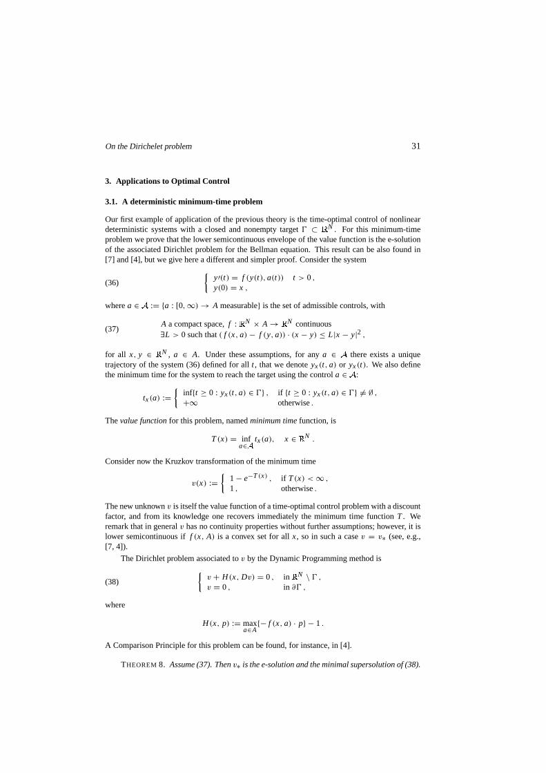
3.1. A deterministic minimum-time problem
Our first example of application of the previous theory is thetime-optimal control of nonlineardeterministic systems with a closed and nonempty target0 ⊂ �N . For this minimum-timeproblem we prove that the lower semicontinuous envelope of the value function is the e-solutionof the associated Dirichlet problem for the Bellman equation. This result can be also found in[7] and [4], but we give here a different and simpler proof. Consider the system
{
y′(t) = f (y(t),a(t)) t > 0 ,
y(0) = x ,(36)
wherea ∈ � := {a : [0, ∞) → A measurable} is the set of admissible controls, with
A a compact space,f :�N × A → �N continuous
∃L > 0 such that( f (x, a) − f (y, a)) · (x − y) ≤ L |x − y|2 ,(37)
for all x, y ∈ �N , a ∈ A. Under these assumptions, for anya ∈ � there exists a uniquetrajectory of the system (36) defined for allt , that we denoteyx(t, a) or yx(t). We also definethe minimum time for the system to reach the target using the control a ∈ � :
tx(a) :={
inf{t ≥ 0 : yx(t,a) ∈ 0} , if {t ≥ 0 : yx(t, a) ∈ 0} 6= ∅ ,
+∞ otherwise.
Thevalue functionfor this problem, namedminimum timefunction, is
T(x) = infa∈�
tx(a), x ∈ �N .
Consider now the Kruzkov transformation of the minimum time
v(x) :={
1 − e−T(x) , if T(x) < ∞ ,
1 , otherwise.
The new unknownv is itself the value function of a time-optimal control problem with a discountfactor, and from its knowledge one recovers immediately theminimum time functionT . Weremark that in generalv has no continuity properties without further assumptions;however, it islower semicontinuous iff (x, A) is a convex set for allx, so in such a casev = v∗ (see, e.g.,[7, 4]).
The Dirichlet problem associated tov by the Dynamic Programming method is
{
v + H(x, Dv) = 0 , in�N \ 0 ,
v = 0 , in ∂0 ,(38)
where
H(x, p) := maxa∈A
{− f (x, a) · p} − 1 .
A Comparison Principle for this problem can be found, for instance, in [4].
THEOREM 8. Assume (37). Thenv∗ is the e-solution and the minimal supersolution of (38).
32 M. Bardi – S. Bottacin
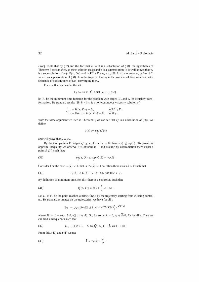
Proof. Note that by (37) and the fact thatw ≡ 0 is a subsolution of (38), the hypotheses ofTheorem 3 are satisfied, so the e-solution exists and it is a supersolution. It is well known thatv∗
is a supersolution ofv + H(x, Dv) = 0 in�N \ 0, see, e.g., [28, 8, 4]; moreoverv∗ ≥ 0 on∂0,
sov∗ is a supersolution of (38). In order to prove thatv∗ is the lower e-solution we construct asequence of subsolutions of (38) converging tov∗.
Fix ε > 0, and consider the set
0ε := {x ∈ �N : dist(x, ∂0) ≤ ε} ,
let Tε be the minimum time function for the problem with target0ε , andvε its Kruzkov trans-formation. By standard results [28, 8, 4]vε is a non-continuous viscosity solution of
{
v + H(x, Dv) = 0 , in�N \ 0ε ,
v = 0 orv + H(x, Dv) = 0 , in ∂0ε .
With the same argument we used in Theorem 6, we can see thatv∗ε is a subsolution of (38). We
define
u(x) := supε
v∗ε (x)
and will prove thatu = v∗.
By the Comparison Principlev∗ε ≤ v∗ for all ε > 0, thenu(x) ≤ v∗(x). To prove the
opposite inequality we observe it is obvious in0 and assume by contradiction there exists apoint x 6∈ 0 such that:
supε
vε (x) ≤ supε
v∗ε (x) < v∗(x) .(39)
Consider first the casev∗(x) < 1, that is,T∗(x) < +∞. Then there existsδ > 0 such that
T∗ε (x) < T∗(x) − δ < +∞, for all ε > 0 .(40)
By definition of minimum time, for allε there is a controlaε such that
tεx (aε ) ≤ Tε (x) + δ
2< +∞ .(41)
Let zε ∈ 0ε be the point reached at timetεx (aε) by the trajectory starting fromx, using controlaε . By standard estimates on the trajectories, we have for allε
|zε | = |yx(tεx (aε))| ≤(
|x| +√
2MT(x)
)
eMT (x) ,
whereM := L + sup{| f (0, a)| : a ∈ A}. So, for someR > 0, zε ∈ B(0, R) for all ε. Then wecan find subsequences such that
zεn → z ∈ ∂0, tn := tεnx (aεn) → t, asn → ∞ .(42)
From this, (40) and (41) we get
t < T∗(x) − δ
2.(43)
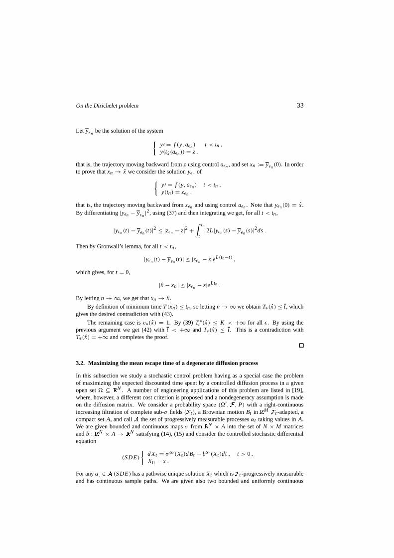
On the Dirichelet problem 33
Let yεn be the solution of the system
{
y′ = f (y, aεn) t < tn ,
y(tx(aεn)) = z ,
that is, the trajectory moving backward fromz using controlaεn , and setxn := yεn(0). In orderto prove thatxn → x we consider the solutionyεn of
{
y′ = f (y, aεn) t < tn ,
y(tn) = zεn ,
that is, the trajectory moving backward fromzεn and using controlaεn . Note thatyεn(0) = x.By differentiating|yεn − yεn |2, using (37) and then integrating we get, for allt < tn,
|yεn(t) − yεn(t)|2 ≤ |zεn − z|2 +∫ tn
t2L |yεn(s) − yεn(s)|2ds.
Then by Gronwall’s lemma, for allt < tn,
|yεn(t) − yεn(t)| ≤ |zεn − z|eL(tn−t) ,
which gives, fort = 0,
|x − xn| ≤ |zεn − z|eLtn .
By lettingn → ∞, we get thatxn → x.
By definition of minimum timeT(xn) ≤ tn, so lettingn → ∞ we obtainT∗(x) ≤ t , whichgives the desired contradiction with (43).
The remaining case isv∗(x) = 1. By (39) T∗ε (x) ≤ K < +∞ for all ε. By using the
previous argument we get (42) witht < +∞ and T∗(x) ≤ t . This is a contradiction withT∗(x) = +∞ and completes the proof.
3.2. Maximizing the mean escape time of a degenerate diffusion process
In this subsection we study a stochastic control problem having as a special case the problemof maximizing the expected discounted time spent by a controlled diffusion process in a givenopen set� ⊆ �N . A number of engineering applications of this problem are listed in [19],where, however, a different cost criterion is proposed and anondegeneracy assumption is madeon the diffusion matrix. We consider a probability space(�′,� , P) with a right-continuousincreasing filtration of complete sub-σ fields{� t }, a Brownian motionBt in
�M � t -adapted, acompact setA, and call� the set of progressively measurable processesαt taking values inA.We are given bounded and continuous mapsσ from
�N × A into the set ofN × M matricesandb :
�N × A → �N satisfying (14), (15) and consider the controlled stochastic differentialequation
(SDE)
{
d Xt = σαt (Xt )d Bt − bαt (Xt )dt , t > 0 ,
X0 = x .
For anyα. ∈ � (SDE) has a pathwise unique solutionXt which is� t -progressively measurableand has continuous sample paths. We are given also two bounded and uniformly continuous
34 M. Bardi – S. Bottacin
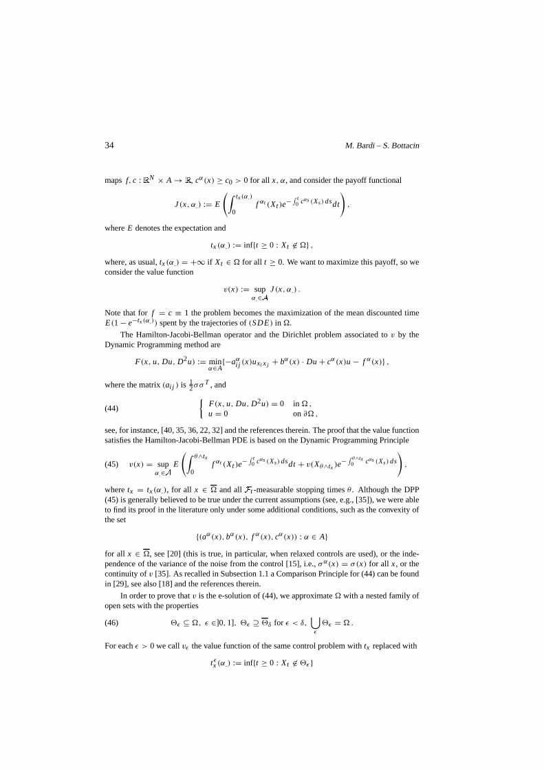
maps f, c :�N × A → �
, cα(x) ≥ c0 > 0 for all x, α, and consider the payoff functional
J(x, α.) := E
(
∫ tx(α.)
0f αt (Xt )e
−∫ t
0 cαs(Xs) dsdt
)
,
whereE denotes the expectation and
tx(α.) := inf{t ≥ 0 : Xt 6∈ �} ,
where, as usual,tx(α.) = +∞ if Xt ∈ � for all t ≥ 0. We want to maximize this payoff, so weconsider the value function
v(x) := supα.∈�
J(x, α.) .
Note that for f = c ≡ 1 the problem becomes the maximization of the mean discounted timeE(1 − e−tx(α.)) spent by the trajectories of(SDE) in �.
The Hamilton-Jacobi-Bellman operator and the Dirichlet problem associated tov by theDynamic Programming method are
F(x, u, Du, D2u) := minα∈A
{−aαi j (x)uxi x j + bα(x) · Du + cα(x)u − f α(x)} ,
where the matrix(ai j ) is 12σσ T , and
{
F(x, u, Du, D2u) = 0 in �,
u = 0 on∂� ,(44)
see, for instance, [40, 35, 36, 22, 32] and the references therein. The proof that the value functionsatisfies the Hamilton-Jacobi-Bellman PDE is based on the Dynamic Programming Principle
v(x) = supα.∈�
E
(
∫ θ∧tx
0f αt (Xt )e
−∫ t
0 cαs (Xs) dsdt + v(Xθ∧tx )e−∫ θ∧tx
0 cαs (Xs) ds
)
,(45)
wheretx = tx(α.), for all x ∈ � and all� t -measurable stopping timesθ . Although the DPP(45) is generally believed to be true under the current assumptions (see, e.g., [35]), we were ableto find its proof in the literature only under some additionalconditions, such as the convexity ofthe set
{(aα(x), bα(x), f α(x), cα(x)) : α ∈ A}
for all x ∈ �, see [20] (this is true, in particular, when relaxed controls are used), or the inde-pendence of the variance of the noise from the control [15], i.e.,σα(x) = σ(x) for all x, or thecontinuity ofv [35]. As recalled in Subsection 1.1 a Comparison Principle for (44) can be foundin [29], see also [18] and the references therein.
In order to prove thatv is the e-solution of (44), we approximate� with a nested family ofopen sets with the properties
2ε ⊆ �, ε ∈]0, 1], 2ε ⊇ 2δ for ε < δ,⋃
ε
2ε = � .(46)
For eachε > 0 we callvε the value function of the same control problem withtx replaced with
tεx (α.) := inf{t ≥ 0 : Xt 6∈ 2ε}
On the Dirichelet problem 35
in the definition of the payoffJ. In the next theorem we assume that eachvε satisfies the DPP(45) with tx replaced withtεx .
Finally, we make the additional assumption
f α(x) ≥ 0 for all x ∈ �, α ∈ A .(47)
which ensures thatu ≡ 0 is a subsolution of (44). The main result of this subsectionis thefollowing.
THEOREM 9. Under the previous assumptions the value functionv is the e-solution and theminimal supersolution of (44), and
v = sup0<ε≤1
vε = limε↘0
vε .
Proof. Note thatvε is nondecreasing asε ↘ 0, so limε↘0 vε exists and equals the sup. ByTheorem 3 withg ≡ 0, u ≡ 0, there exists the e-solutionH0 of (44). We consider the functionsuε defined by (20) and claim that
u2ε ≤ (vε)∗ ≤ v∗ε ≤ H0 .
Then
H0 = sup0<ε≤1
vε ,(48)
becauseH0 = supε u2ε by Remark 1. We prove the claim in three steps.
Step 1. By standard methods [35, 9], the Dynamic ProgrammingPrinciple forvε impliesthatvε is a non-continuous viscosity solution of the Hamilton-Jacobi-Bellman equationF = 0in 2ε andv∗
ε is a viscosity subsolution of the boundary condition
u = 0 or F(x, u, Du, D2u) = 0 on∂2ε ,(49)
as defined in Subsection 1.3.
Step 2. Since(vε )∗ is a supersolution of the PDEF = 0 in 2ε and(vε )∗ ≥ 0 on∂2ε , theComparison Principle implies(vε)∗ ≥ w for any subsolutionw of (44) such thatw = 0 on∂2ε .Since∂2ε ⊆ � \ 22ε by (46), we obtainu2ε ≤ vε∗ by the definition (20) ofu2ε .
Step 3. We claim thatv∗ε is a subsolution of (44). In fact we noted before that it is a
subsolution of the PDE in2ε , and this is true also in� \ 2ε wherev∗ε ≡ 0 by (47), whereas the
boundary condition is trivial. It remains to check the PDE atall points of∂2ε . Given x ∈ ∂2ε ,we must prove that for allφ ∈ C2(�) such thatv∗
ε − φ attains a local maximum atx, we have
F(x, v∗ε (x), Dφ(x), D2φ(x)) ≤ 0 .(50)
1st Case:v∗ε (x) > 0. Sincev∗
ε satisfies (49), for allφ ∈ C2(2ε) such thatv∗ε − φ attains a
local maximum atx (50) holds. Then the same inequality holds for allφ ∈ C2(�) as well.
2nd Case:v∗ε (x) = 0. Sincev∗
ε − φ attains a local maximum atx, for all x nearx we have
v∗ε (x) − v∗
ε (x) ≤ φ(x) − φ(x) .
By Taylor’s formula forφ at x and the fact thatv∗ε (x) ≥ 0, we get
Dφ(x) · (x − x) ≥ o(|x − x|) ,
36 M. Bardi – S. Bottacin
and this impliesDφ(x) = 0. Then Taylor’s formula forφ gives also
(x − x) · D2φ(x)(x − x) ≥ o(|x − x|2) ,
and this impliesD2φ(x) ≥ 0, as it is easy to check. Then
F(x, v∗ε (x), Dφ(x), D2φ(x)) = F(x, 0, 0, D2φ(x)) ≤ 0
becauseaα ≥ 0 and f α ≥ 0 for all x andα. This completes the proof thatv∗ε is a subsolution of
(44). Now the Comparison Principle yieldsv∗ε ≤ H0, sinceH0 is a supersolution of (44).
It remains to prove thatv = sup0<ε≤1 vε . To this purpose we take a sequenceεn ↘ 0 anddefine
Jn(x, α.) := E
(
∫ tεnx (α.)
0f αt (Xt )e
−∫ t
0 cαs (Xs) dsdt
)
.
We claim that
limn
Jn(x, α.) = supn
Jn(x, α.) = J(x, α.) for all α. andx .
The monotonicity oftεnx follows from (46) and it implies the monotonicity ofJn by (47). Let
τ := supn
tεnx (α.) ≤ tx(α.) ,
and note thattx(α.) = +∞ if τ = +∞. In the caseτ < +∞, Xtεnx
∈ ∂2εn implies Xτ ∈ ∂�,so τ = tx(α.) again. This and (47) yield the claim by the Lebesgue monotoneconvergencetheorem. Then
v(x) = supα.
supn
Jn(x, α.) = supn
supα.
Jn(x, α.) = supn
vεn = supε
vε ,
so (48) givesv = H0 and completes the proof.
REMARK 7. From Theorem 9 it is easy to get aVerification theoremby taking the su-persolutions of (44) as verification functions. We considera presynthesisα(x), that is, a mapα(·) : � → � , and say it is optimal atxo if J(xo, α
(xo)) = v(xo). Then Theorem 9 gives im-mediately the following sufficient condition of optimality: if there exists a verification functionW such that W(xo) ≤ J(xo, α(xo)), thenα(·) is optimal at xo; moreover, a characterization ofglobal optimality is the following:α(·) is optimal in� if and only if J(·, α(·)) is a verificationfunction.
REMARK 8. We can combine Theorem 9 with the results of Subsection 2.2to approximatethe value functionv with smooth value functions. Consider a Brownian motionBt in
�N � t -adapted and replace the stochastic differential equation in (SDE) with
d Xt = σαt (Xt )d Bt − bαt (Xt )dt +√
2h dBt , t > 0 ,
for h > 0. For a family of nested open sets with the properties (46) consider the value functionvε
h of the problem of maximizing the payoff functionalJ with tx replaced withtεx . Assume forsimplicity thataα , bα , cα , f α are smooth (otherwise we can approximate them by mollification).Thenvε
h is the classical solution of (30), whereF is the HJB operator of this subsection andu ≡ 0, by the results in [21, 24, 36, 31], and it is possible to synthesize an optimal Markovcontrol policy for the problem withε,h > 0 by standard methods (see, e.g., [22]). By Theorem6 vε
h converges tov asε, h ↘ 0 with h linked toε.
On the Dirichelet problem 37
References
[1] BARDI M., BOTTACIN S., Discontinuous solution of degenerate elliptic boundary valueproblems, Preprint 22, Dip. di Matematica P. e A., Universita di Padova, 1995.
[2] BARDI M., BOTTACIN S., Characteristic and irrelevant boundary points for viscositysolutons of nonlinear degenerate elliptic equations, Preprint 25, Dip. di Matematica P. eA., Universita di Padova, 1998.
[3] BARDI M., BOTTACIN S., FALCONE M., Convergence of discrete schemes for discontin-uous value functions of pursuit-evasion games, in “New Trends in Dynamic Games andApplications”, G .J. Olsder ed., Birkhauser, Boston 1995,273–304.
[4] BARDI M., CAPUZZO-DOLCETTA I., Optimal control and viscosity solutions of Hamilton-Jacobi-Bellman equations, Birkhauser, Boston 1997.
[5] BARDI M., CRANDALL M., EVANS L. C., SONER H. M., SOUGANIDIS P. E.,Viscositysolutions and applications, I. Capuzzo Dolcetta and P.-L. Lions eds., Springer LectureNotes in Mathematics 1660, Berlin 1997.
[6] BARDI M., GOATIN P., ISHII H., A Dirichlet type problem for nonlinear degenerate ellip-tic equations arising in time-optimal stochastic control, Preprint 1, Dip. di Matematica P. eA., Universita di Padova, 1998, to appear in Adv. Math. Sci.Appl.
[7] BARDI M., STAICU V., The Bellman equation for time-optimal control of noncontrollable,nonlinear systems, Acta Appl. Math.31 (1993), 201–223.
[8] BARLES G., Solutions de viscosite des equations de Hamilton-Jacobi, Springer-Verlag,1994.
[9] BARLES G., BURDEAU J.,The Dirichlet problem for semilinear second-order degenerateelliptic equations and applications to stochastic exit time control problems, Comm. PartialDifferential Equations20 (1995), 129–178.
[10] BARLES G., PERTHAME B., Discontinuous solutions of deterministic optimal stoppingtime problems, RAIRO Model. Math. Anal. Numer21 (1987), 557–579.
[11] BARRON E. N., JENSENR., Semicontinuous viscosity solutions of Hamilton-Isaacs equa-tion with convex Hamiltonians, Comm. Partial Differential Equations15 (1990), 1713–1742.
[12] BERESTYCKI H., NIRENBERG L., VARADHAN S. R. S.,The Principal Eigenvalue andMaximum Principle for Second-Order Elliptic Operators in General Domains, Comm.Pure App. Math.XLVII (1994), 47–92.
[13] BETTINI P.,Problemi di Cauchy per equazioni paraboliche degeneri con dati discontinuie applicazioni al controllo e ai giochi differenziali, Thesis, Universita di Padova, 1998.
[14] BLANC A.-PH., Deterministic exit time control problems with discontinuous exit costs,SIAM J. Control Optim.35 (1997), 399–434.
[15] BORKAR V. S., Optimal control of diffusion processes, Pitman Research Notes in Mathe-matics Series203, Longman, Harlow 1989.
[16] BRELOT M., Familles de Perron et probleme de Dirichlet, Acta Litt. Sci. Szeged9 (1939),133–153.
[17] CAFFARELLI L. A., CABRE X., Fully nonlinear elliptic equations, Amer. Math. Soc.,Providence, RI, 1995.
38 M. Bardi – S. Bottacin
[18] CRANDALL M. C., ISHII H., LIONS P. L., User’s guide to viscosity solutions of secondorder partial differential equations, Bull. Amer. Math. Soc.27 (1992), 1–67.
[19] DUPUISP., MCENEANEY W. M., Risk-sensitive and robust escape criteria, SIAM J. Con-trol Optim.35 (1997), 2021–2049.
[20] EL KAROUI N., HUU NGUYEN D., JEANBLANC-PICQUE M., Compactification methodsin the control of degenerate diffusions: existence of an optimal control, Stochastics20(1987), 169–219.
[21] EVANS L. C., Classical solutions of the Hamilton-Jacobi-Bellman equation for unifor-mally elliptic operators, Trans. Amer. Math. Soc.275(1983), 245–255.
[22] FLEMING W. H., SONER H. M., Controlled Markov Process and Viscosity Solutions,Springer-Verlag, New York 1993.
[23] FREIDLIN M., Functional integration and partial differential equations, Princeton Univer-sity Press, Princeton 1985.
[24] GILBARG D., TRUDINGERN. S.,Elliptic Partial Differential Equations of Second Order,2nd ed. Springer-Verlag, Berlin 1983.
[25] HEINONEN J., KILPELAINEN T., MARTIO O., Nonlinear Potential Theory of DegenerateElliptic Equations, Oxford Science Publications, Clarendon Press, Oxford 1993.
[26] HELMS L. L., Introduction to Potential Theory, Wiley-Interscience, New York 1969.
[27] ISHII H., Perron’s method for Hamilton-Jacobi equations, Duke Math. J.55 (1987), 369–384.
[28] ISHI H., A boundary value problem of the Dirichlet type for Hamilton-Jacobi equations,Ann. Scuola Norm. Sup. Pisa16 (1986), 105–135.
[29] JENSEN R., Uniqueness criteria for viscosity solutions of fully nonlinear elliptic partialdifferential equations, Indiana Univ. Math. J.38 (1989), 629–667.
[30] KELLOGG O. D.,Foundations of Potential Theory, Verlag-Springer, Berlin 1929.
[31] KRYLOV N. V., Nonlinear Elliptic and Parabolic Equations of the Second Order, D. ReidelPublishing Company, Dordrecht 1987.
[32] KRYLOV N. V., Smoothness of the payoff function for a controllable process in a domain,Math. USSR-Izv.34 (1990), 65–95.
[33] KRYLOV N. V., Lectures on elliptic and parabolic equations in Holder spaces, GraduateStudies in Mathematics, 12, American Mathematical Society, Providence, RI, 1996.
[34] L IONS P. L.,Generalized solutions of Hamilton-Jacobi equations, Pitman, Boston 1982.
[35] L IONS P. L., Optimal control of diffusion processes and Hamilton-Jacobi-Bellman equa-tions. Part 1: The dynamic programming principle and applications, Part 2: Viscositysolutions and uniqueness, Comm. Partial. Differential Equations8 (1983), 1101–1174 and1229–1276.
[36] L IONS P.-L.,Optimal control of diffusion processes and Hamilton-Jacobi-Bellman equa-tions. III - Regularity of the optimal cost function, in “Nonlinear partial differential equa-tions and applications”, College de France seminar, Vol. V(Paris 1981/1982), 95–205, Res.Notes in Math., 93, Pitman, Boston, Mass.-London 1983.
[37] OLEINIK O. A., RADKEVIC E. V., Second order equations with nonnegative characteris-tic form, Plenum Press, New York 1973.
On the Dirichelet problem 39
[38] RAMASWAMY M., RAMASWAMY S., Perron’s method and barrier functions for the vis-cosity solutions of the Dirichlet problem for some nonlinear partial differential equations,Z. Anal. Anwendungen13 (1994), 199–207.
[39] SORAVIA P.,Discontinuous viscosity solutions to Dirichlet problems for Hamilton-Jacobiequations with convex Hamiltonians, Comm. Partial Diff. Equations18(1993), 1493–1514.
[40] STROOCK D., VARADHAN S. R. S.,On Degenerate Elliptic-Parabolic Operators of Sec-ond Order and Their Associated Diffusions, Comm. Pure App. Math.XXV (1972), 651–713.
[41] SUBBOTIN A. I., Discontinuous solutions of a Dirichlet type boundary valueproblem forfirst order P.D.E., Russian Numer. Anal. Math. Modelling J.8 (1993), 145–164.
[42] SUBBOTIN A. I., Generalized solutions of first order PDEs: The Dynamic OptimizationPerspective, Birkhauser, Boston 1995.
[43] TRUDINGERN. S.,On the twice differentiability of viscosity solutions of nonlinear ellipticequations, Bull. Austral. Math. Soc.39 (1989), 443–447.
[44] WIENER N., Certain notions in Potential Theory, J. Math. Phys. (M.I.T.)3 (1924), 24–51.
[45] WIENER N., Note on a paper of O. Perron, J. Math. Phys. (M.I.T.)4 (1925), 21–32.
AMS Subject Classification: ???.
Martino BARDI, Sandra BOTTACINDipartimento di Matematica P. e A.Universita di Padovavia Belzoni 7, I-35131 Padova, Italy

40 M. Bardi – S. Bottacin