,'m FILE COPY

NFROM: AFIT/CI 31 Jan 90

0 SUBJ: Review of Thesis/Disseration for Public Release

NTO: PA

Request you review the attached for public release prior to beingsent to DTIC.

ERNEST A. HAYWOOD, 1st Lt, USAF 1 AtchExecutive officer ThesisCivilian Institution Programs D derANbrioKx

by Hofmann

1st Ind, AFIT/PA FES

TO: CI

Approved/Pis-pproyed for public release.Log Number: 89-185

P)~IAALd 6 M VX&HARRIET D. MOULTRIE, Capt, USAFDirector, Office of Public Affairs

DTICA" ELECTE

FEB 22 1990 13

90 C21

SECURITY CLASSIFICATION OF THIS PAGE

Form ApprovedREPORT DOCUMENTATION PAGE OMBNo. 0704-0188

la. REPORT SECURITY CLASSIFICATION lb. RESTRICTIVE MARKINGSUNCLASSIFIED NONE

2a. SECURITY CLASSIFICATION AUTHORITY 3. DISTRIBUTION /AVAILABILITY OF REPORTAPPROVED FOR PUBLIC RELEASE;

2b. DECLASSIFICATION /DOWNGRADING SCHEDULE DISTRIBUTION UNLIMITED.

4. PERFORMING ORGANIZATION REPORT NUMBER(S) 5. MONITORING ORGANIZATION REPORT NUMBER(S)

AFIT/CI/CIA- 8 9 - 18 5

6a. NAME OF PERFORMING ORGANIZATION 6b. OFFICE SYMBOL 7a. NAME OF MONITORING ORGANIZATIONAFIT STUDENT AT (If applicable) AFIT/CIAPENNSYLVANIA STATE UNIV

6c. ADDRESS (City, State, and ZIP Code) 7b. ADDRESS (City, State, and ZIP Code)

Wright-Patterson AFB OH 45433-6583

8a. NAME OF FUNDING/SPONSORING Bb. OFFICE SYMBOL 9. PROCUREMENT INSTRUMENT IDENTIFICATION NUMBERORGANIZATION (If applicable)

8c. ADDRESS (City, State, and ZIP Code) 10. SOURCE OF FUNDING NUMBERSPROGRAM PROJECT TASK WORK UNITELEMENT NO. NO. NO ACCESSION NO.

11. TITLE (Include Security Classification) (UNCLASSIFIED)

OPTIMAL ALLOGATION AND STATISTICAL CONTROL OF ASSEMBLY PROCESSES

12. PERSONAL AUTHOR(S)

PETER J. HOFMANN13a. TYPE OF REPORT 113b. TIME COVERED 114. DATE OF REPORT (Year, Month, Day) 15. PAGE COUNTTHESIS/V 3XI FROM TO / 1989 1 3816. SUPPLEMENTARY NOTATION APFRUVE1 FOR PUBLIC RELEASE lAW AFR 190-1

ERNEST A. HAYGOOD, 1st Lt, USAFExecutive Officer, Civilian Institution Programs

17. COSATI CODES 18. SUBJECT TERMS (Continue on reverse if necessary and identify by block number)FIELD GROUP SUB-GROUP

19. ABSTRACT (Continue on reverse if necessary and identify by block number)

20. DISTRIBUTION/AVAILABILITY OF ABSTRACT 21. ABSTRACT SECURITY CLASSIFICATION[3UNCLASSIFIED/UNLMITED 0 SAME AS RPT. C DTIC USERS UNCLASSIFIED

22a. NAME OF RESPONSIBLE IND.VIDUAL 22b. TELEPHONE (Include Area Code) 22c. OFFICE SYMBOLERNEST A. HAYGOOD, 1st Lt, USAF (513) 255-2259 AFIT/CI

DD Form 1473, JUN 86 Previous editions are obsolete. SECURITY CLASSIFICATION OF THIS PAGE

AFIT/CI "OVERPRINT"

The Pennsylvania State University

The Graduate School

OPTIMAL ALLOCATION AND STATISTICAL CONTROL

OF ASSEMBLY PROCESSES

A Thesis in

Industrial Engineering and Operations Research

by

Peter J. Hofmann

Submitted in Partial Fulfillmentof the Requirementsfor the Degree of Accession For

N _ T I S _ _ G R A & I - -DTIC TABUnannounced

Master of Science t

By-Distribution/

May 1990 AvailabilitY Codes

jAv;.il ,,ndlorDist Spccial

I grant The Pennsylvania State University thenonexclusive right to use this work for theUniversity's own purposes and to make singlecopies of the work available to the public ona not-for-profit basis if copies are nototherwise available.

Peter J. Hofmann

We approve the thesis of Peter J. Hofmann.

Date of Signature

M. Jea'~daAssociate Professor of

Industrial EngineeringThesis Advisor

Kalyan ChatterjeeProfessor of Management Science

Allen L. Soy erProfessor of Industrial EngineeringHead of the Department of Industrial

and Management Systems Engineering

i iii

ABSTRACT

An analytic procedure was developed to predict the expected

proportion of defectives produced, using a specified set of

fabrication and assembly processes. This procedure was demonstrated

for a General assembly process, a Peg-in-Hole assembly process and a

Box-and-Cover assembly process. This procedure was compared to the

formulation of a Monte Carlo simulation model and shown to require

the same initial information. Two applications of the results of

this procedure were developed..The first was an optimization model

used to allocate a fixed amount of capital improvements to a discrete

number of possible candidate assembly processes. The second was to

statistically control an assembly process using a p Chart. A

numerical example illustrating the procedure and its applications was

also presented.

r _ . ..

/

iv

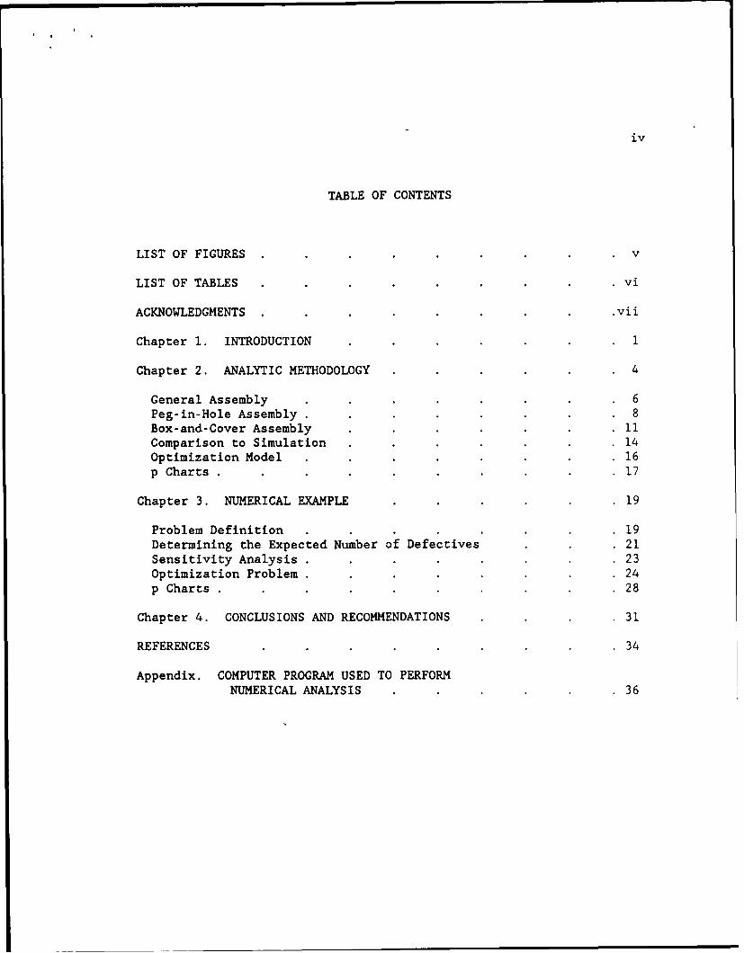
TABLE OF CONTENTS

LIST OF FIGURES v

LIST OF TABLES . vi

ACKNOWLEDGMENTS . vii

Chapter 1. INTRODUCTION 1

Chapter 2. ANALYTIC METHODOLOGY 4

General Assembly 6

Peg-in-Hole Assembly . 8Box-and-Cover Assembly 11Comparison to Simulation 14

Optimization Model 16

p Charts . 17

Chapter 3. NUMERICAL EXAMPLE 19

Problem Definition 19

Determining the Expected Number of Defectives 21

Sensitivity Analysis . 23Optimization Problem . 24p Charts 28

Chapter 4. CONCLUSIONS AND RECOMMENDATIONS 31

REFERENCES 34

Appendix. COMPUTER PROGRAM USED TO PERFORMNUMERICAL ANALYSIS 36

v

LIST OF FIGURES

2.1. General Assembly 7

2.2. Peg-in-Hole Assembly 9

2.3. Box-and-Cover Assembly . 12

3.1. Numerical Example 20

3.2. Sample p Chart 30

vi

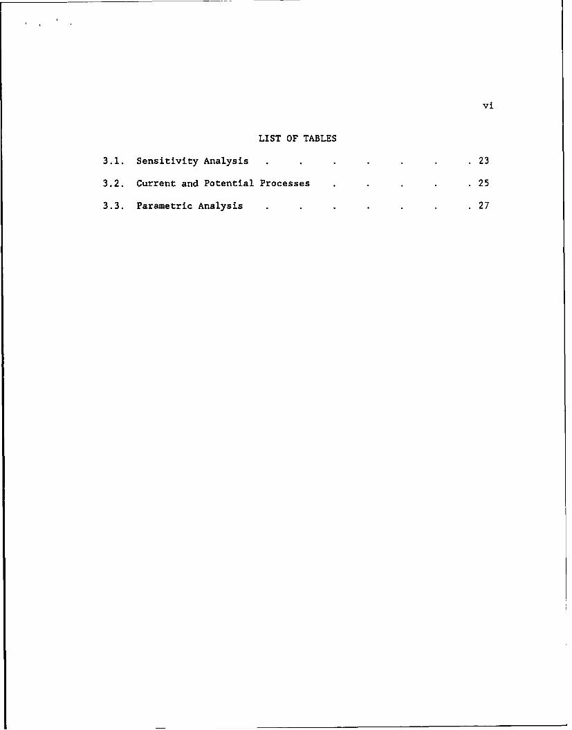
LIST OF TABLES

3.1. Sensitivity Analysis . 23

3.2. Current and Potential Processes 25

3.3. Parametric Analysis 27

vii

ACKNOWLEDGMENTS

I want to express my sincere appreciation to my advisor, Dr.

Jeya Chandra, for his help in completing this paper. His patience,

encouragement and desire to enlighten his students serves as an

example for all educators to emulate. I am also greatful to Dr. Tom

Cavalier for his assistance with the optimization portions of this

paper. I feel very fortunate to have had teachers like Dr. Chandra

and Dr. Cavalier for several of my courses. I learned a great deal

from both of these professors.

I also want to thank my wife, Theresa, for her support and

encouragement through the course of my studies. She was also a

tremendous help during the preparation of this thesis, more than she

probably realizes. She is and always will be my best friend.

1

Chapter 1

INTRODUCTION

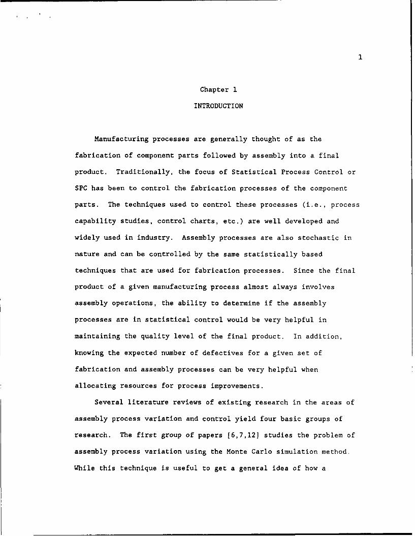
Manufacturing processes are generally thought of as the

fabrication of component parts followed by assembly into a final

product. Traditionally, the focus of Statistical Process Control or

SPC has been to control the fabrication processes of the component

parts. The techniques used to control these processes (i.e., process

capability studies, control charts, etc.) are well developed and

widely used in industry. Assembly processes are also stochastic in

nature and can be controlled by the same statistically based

techniques that are used for fabrication processes. Since the final

product of a given manufacturing process almost always involves

assembly operations, the ability to determine if the assembly

processes are in statistical control would be very helpful in

maintaining the quality level of the final product. In addition,

knowing the expected number of defectives for a given set of

fabrication and assembly processes can be very helpful when

allocating resources for process improvements.

Several literature reviews of existing research in the areas of

assembly process variation and control yield four basic groups of

research. The first group of papers [6,7,12] studies the problem of

assembly process variation using the Monte Carlo simulation method.

While this technique is useful to get a general idea of how a

2

complete manufacturing process operates, it does not lend itself to

the problem of optimally allocating capital improvements or real time

process control. Another group of papers [8,9,10,11,14] considers

the effect of assembly errors on circular arc or Novikov types of

gears. These papers consider the assembly errors to be deterministic

and measurable for a given gear pair. This analysis is useful for

failure mode analysis and other preliminary design related tasks, but

not for true manufacturing and quality control applications.

The final two groups of research are more closely related to the

main thrust of this paper. The first of these groups is research

into the allocation of errors in hierarchical calibration or assembly

systems. Rajaraman [13] expands Crow's work [3,4] on calibration

systems to assembly systems. Rajaraman develops a dynamic

programming model to optimally allocate resources to each stage of

assembly. The main drawback to this approach is that the assembly

variations at each stage have to be independent to use a dynamic

programming approach. While this is true for the linear or

"telescopic" assembly process described in [13], it isn't true for a

general or "tree-like" assembly process. The problem given in

Chapter 3 of this paper is an example of a "tree-like" assembly

process since the assembly variations in the third stage are

dependent on the variations in the first stage. Rajaraman also

illustrates that the manner in which errors propagate between stages

is unknown and can be assumed to be a linear or nonlinear function.

The last group of research related to assembly process variation

3

is the analysis of basic assembly operations, used in the

implementation of robotic or automated assembly stations. While

there are a large number of papers to choose from, the works by

Abdel-Malek [1] and Boucher [2] are used for their clear analyses of

the two most basic assemblies, Peg-in-Hole and Box-and-Cover. Both

authors develop probabilistic relationships for successful completion

of both of these assembly operations. Their research concentrates on

the probability of a robot with known repeatability being able to

insert a peg into a hole or a box into a cover. They do not consider

the geometries of the actual parts that are assembled and whether

these parts are assembled within acceptable tolerances.

There are three basic objectives of this paper. The first

objective is to analytically predict the expected number of defective

units for a given set of fabrication and assembly processes. This

will be accomplished using the same probabilistic analysis used for a

Monte Carlo type of simulation except that the results will be

determined using numerical integration and not simulation. The next

objective is to develop an optimization model to allocate a limited

amount of capital resources to reduce the variation in the existing

assembly processes. Finally, a method for statistically controlling

an assembly process is developed.

4

Chapter 2

ANALYTIC METHODOLOGY

The basic approach used in this method is to analyze a given

assembly process from a probabilistic viewpoint. There are three

basic probabilities associated with any assembly process. First,

there is the probability that assembly is possible. For example, it

is possible that machined components will not fit together even if

there is no assembly process variation. The next event of interest

is the probability that assembly will be successful in light of the

existing assembly process variation. These two probabilities have

been most widely researched for application in robotic assembly, as

mentioned in Chapter 1. Finally, there is the probability that a

successfully assembled unit meets the specified quality requirements.

To have a completed assembly with the required quality, all three of

these probabilities have to be satisfied.

As stated in Chapter 1, the most common methodology used to

obtain an expected number of defective assemblies (i.e., an assembly

that doesn't meet all three conditions above) is the Monte Carlo

Simulation. In this paper, an analytic solution is found using

numerical integration techniques. The method used to find this

solution will be demonstrated on three basic assembly processes. The

first is a General assembly process, one that doesn't contain any

assembly aids (i.e., fixtures, pegs and holes, etc.). Since the

5

assembly variation associated with this process isn't limited by

assembly aids, the assembly variation isn't restricted in any

direction. Next, a Peg-in-Hole assembly will be considered. The

Peg-in-Hole assembly process limits the possible variation in the X

and Y directions. Finally, a Box-and-Cover assembly will be

considered. The Box-and-Cover assembly process is essentially a

rectangular Peg-in-Hole which limits variation in the X, Y and 0

directions. It is assumed during this analysis that only one attempt

is made at assembly. Also, if the assembly is successful, the part

is fixed to the work, capturing the assembly errors.

Finally, a review of the basics of numerical integration

including the definition of some useful notation is appropriate

before beginning the analysis. The general process is to write the

expression of interest as a discrete sum over each of the random

variables in the expression. The limits are either the full range of

the random variable (plus or minus four times the standard deviation

is used as an approximation) or are defined in the expression being

evaluated. Each range can then be partitioned into a discrete number

(say 100) of increments and summed over all of these increments. If

the increment has lower bound Bl and upper bound B2, then the point

estimate (X') used in evaluation the expression is given by:

V - 0.5*(B2 - BI) (1)

The value for the expression being evaluated is then multiplied by

the probability of each of the point estimators occuring, or:

Pr( Bl < X' < B2 ) - Pr(X') (2)

6

This procedure is repeated in a nested loop fashion until all of the

possible values for each random variable have been considered. The

summation expressions that are obtained using this procedure may

appear very complex, but they are easily programmed as a series of

nested loops with a subroutine to compute the Pr(X')'s from equation

(2). The computations are straightforward and easily computed using

any personal computer.

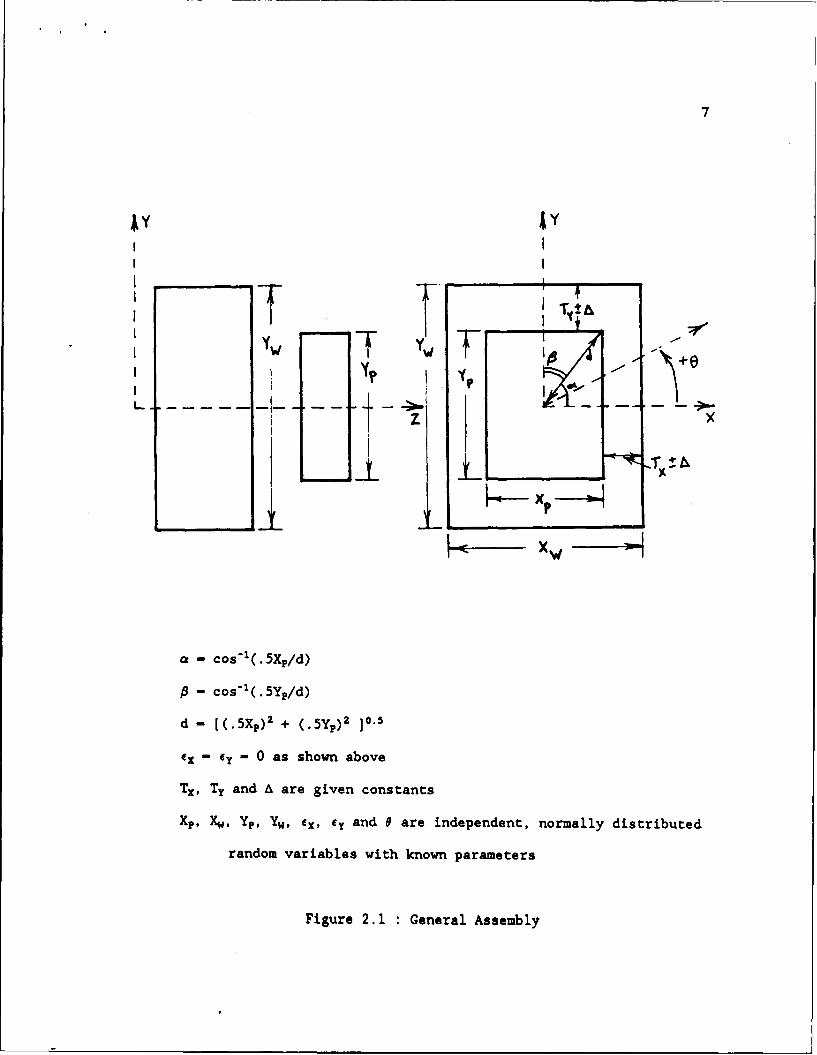
General Assembly

An overview of the General assembly process is given in Figure

2.1. From Figure 2.1, it is clear that the General Assembly process

doesn't have any assembly aids to limit variation in assembly. This

means that any attempt at assembly will be successful. Therefore, if

the completed assembly is within the specified tolerance, it will be

of the required level of quality. Using the nomenclature given in

Figure 2.1, the probability of the part being within the tolerance

limits is given by the intersection of the following statements:

Pr{TX-A<.5Xw- (cx+d*cos (a-e))<Tx+A) (3)

Pr(Tx-A<.5Xw-(ex+d*cos(a+8))<Tx+A) (4)

Pr (Ty-6<. 5Yw- (c y+d*cos (,6-0) )<Ty+A } (5 )

PrTy-A<. 5Yw-(cy+d*cos(#+O))<Ty+A) (6)

Statements (3) through (6) can be rewritten as follows:

Pr(Tx- A+ex+d*cos (a-0O)<. 5Xw<Tx+A+ex+d*cos (a -0)) (7)

Pr(Tx- A+ex+d*cos(a+P)<. 5Xw<Tx+A+ex+d*cos (a+#)) (8)

7

W i

I~ T IJr.

I I

a - Co-( 5Xp/d

I I

ii __

I- i-

- cos'1 (. 5X/d)

- cos-'(. 5Yp/d)

d - [(.5XP)2 + (.5Y,)2 ]0.5

ex - ey - 0 as shown above

Tx, Ty and A are given constants

Xp, Xw, Yp, Yw, x, 6y and 9 are independent, normally distributed

random variables with known parameters

Figure 2.1 : General Assembly

8

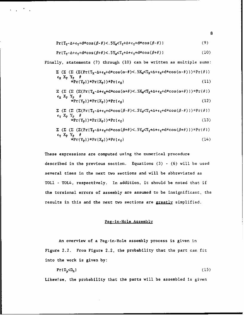
Pr {Ty- A+y+d*cos (f- 0)<. 5Yw<Ty+A+cy+d*cos (f- 0 ) ) (9)

Pr(Ty-A+ey+d*cos(P+O)<. 5Yw<Ty+A+ey+d*cos(0+0) ) (10)

Finally, statements (7) through (10) can be written as multiple sums:

Z (Z (Z (Z(Pr(Tx-A+ x+d*cos(a-O)<.5Xw<Tx+A+ex+d*cos(a-)))*PrtG))X XpYP 9

*Pr(Yp))*Pr(Xp))*Pr(ex) (11)

E (Z (E (E(Pr(Tx-A+ex+d*cos(a+9)<.5Xw<Tx+A+x+d*cos(a+B)))*Pr({))ex Xp Yp 0

*Pr{Yp))*Pr(Xp})*Pr(X)() (12)

Z (E (Z (E(PrtTy-A+ey+d*cos(6-0)<.5Yw<Ty+A+Ey+d*cos(I3-8)))*Pr(9))CY XP Yp 6

*Pr(Yp))*Pr{Xp))*Pr(ey) (13)

E (Z ( (E(Pr(Ty-A+ey+d*cos(P+6)<.5Yw<Ty+A+ey+d*cos(P+O)))*Pr(8))Cy Xp Yp 0

*Pr(Yp))*Pr(Xp))*Pr({y) (14)

These expressions are computed using the numerical procedure

described in the previous section. Equations (3) - (6) will be used

several times in the next two sections and will be abbreviated as

TOLl - TOL4, respectively. In addition, it should be noted that if

the torsional errors of assembly are assumed to be insignificant, the

results in this and the next two sections are greatly simplified.

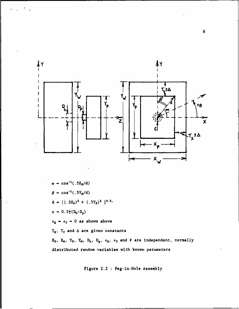
Peg-in-Hole Assembly

An overview of a Peg-in-Hole assembly process is given in

Figure 2.2. From Figure 2.2, the probability that the part can fit

into the work is given by:

Pr(Dp<Dh) (15)

Likewise, the probability that the parts will be assembled is given

9

T V

z x

IPP

a- Cos-'(.5X,,/d)

P- cos 1'(.5Yp/d)

d - [(5P2+ (.5yp) 2 PO.5.

c - O.5t(Dh-DP)

e- ey- 0 as shown above

Tx, Ty and A are given constants

Xjp, Xw, Yp, YW, Dh, DPO ex~, cy and 9 are independent, normally

distributed random variables with known parameters

Figure 2.2 :Peg-in-Hole Assembly

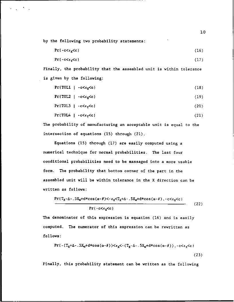
10

by the following two probability statements:

Pr(-c<ex<c) (16)

Pr(-c<ey<c) (17)

Finally, the probability that the assembled unit is within tolerance

is given by the following:

Pr{TOLl -c<ex<c) (18)

Pr{TOL2 -C<Ex<C} (19)

Pr(TOL3 -c<cy<c) (20)

Pr(TOL4 -c<ey<c) (21)

The probability of manufacturing an acceptable unit is equal to the

intersection of equations (15) through (21).

Equations (15) through (17) are easily computed using a

numerical technique for normal probabilities. The last four

conditional probabilities need to be massaged into a more usable

form. The probability that bottom corner of the part in the

assembled unit will be within tolerance in the X direction can be

written as follows:

PrTx- A-.,Xc+d*cos(a-#)<-ex<Tx+A-.5Xw+d*cos(a-0),-C<cx<c)(22)

Pr(-c<ex<c)

The denominator of this expression is equation (16) and is easily

computed. The numerator of this expression can be rewritten as

follows:

Pr(- (Tx+A-.Xw+d*cos(,-))<ex<-(Tx-A-.SXw+d*cos(a-0)),-c<cx<c)

(23)

Finally, this probability statement can be written as the following

multiple sum:

Z (Z (Z ( E(Prmax[-c,-(Tx+A-.5Xw+d*cos(a-0))]<cx<min[c,-(Tx-A-c Xp Yp.5Xw

.5Xw+d*cos(a-0))]))*Pr(.5Xw))*Pr(Yp))*Pr(Xp))*Pr(c)(24)

As with the General assembly, this summation is computed using

the numerical procedure outlined in the first section of this

chapter. The probabilities that the top corner will be within

tolerance in the X direction and both corners in the Y direction

(statements (19)-(21)) are computed in the same manner outlined

above. The probability of producing a defective assembly is computed

in the same manner used for the General assembly process.

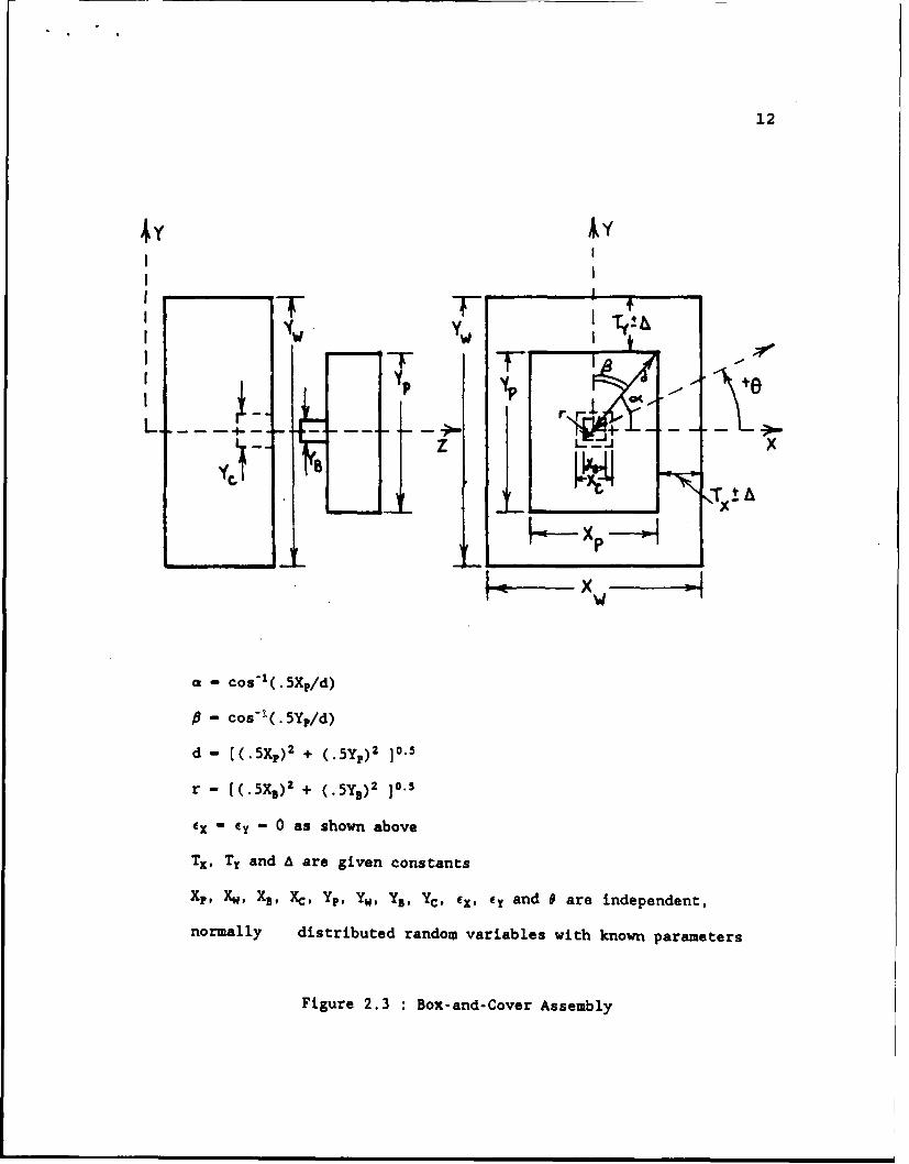
Box-and-Cover Assembly

An overview of a Box and Cover assembly process is presented in

Figure 2.3. Using the notation given in Figure 2.3, the probability

that the part can fit into the work is given by the following two

probability statements:

Pr(Xs<Xc) (25)

Pr(Ys<Yc) (26)

Likewise, the probability that the parts will be assembled on the

first attempt (2] is given by the following probabilities:

Pr({<cos-'(.5XB/r)-cos'l((.5XB+dX)/r) I dX<dY) (27)

Pr({<cos'(.5Y/r)-cos'((.5YB+dY)/r) I dY<dX) (28)

where dX - .5(Xc-Xc)-e x

dY - .5(Yc-Yc)-ey

12

III

III I

T

k- X-

a - cos'1 (.5X1 ,/d)

- cos' (. 5Y,/d)

I d - [(.5X1 )2 + (.5YF) 2 ]0.5

r - [(.5x3) 2 + (.5y1 )2 ]o.5

ex - ¢y- 0 as shown above

T1 , Ty and Al are given constants

Xp, Xwq, X3 , Xc, Y1, Yw, Yu, Yc, EX, Ey and 9 are independent,

normally distributed random variables with known parameters

Figure 2.3 :Box-and-Cover Assembly

ri

13

Finally, the probability that the assembled unit will be within

tolerance is given by the following eight probability statements:

Pr{TOLI e<cosi(.5XB/r)-cos-l((.5XB+dX)/r) ,dX<dY} (29)

Pr{TOLI B<cos'(.5YB/r)-cos-l((.5YB+dY)/r) ,dY<dX) (30)

Pr(TOL2 8<cos'(.5Xs/r)-cos-l((.5XB+dX)/r),dX<dY) (31)

Pr(TOL2 8<cos-(.5YB/r)-cos-1 ((.5YB+dY)/r) ,dY<dX) (32)

Pr(TOL3 8<cos'(.5XB/r)-cos-'((.5XB+dX)/r),dX<dY) (33)

Pr(TOL3 e<cos-(.5YB/r)-cos-1((.5YB+dY)/r),dY<dX) (34)

Pr{TOL4 e<cos-(.5XB/r)-cos-'((.5XB+dX)/r),dX<dY) (35)

Pr(TOL4 e<cos-1 (.5Ys/r)-cos'((.5YB+dY)/r),dY<dX) (36)

The probability of manufacturing an acceptable unit is equal to the

intersection of equations (25) through (36).

The first two equations, (25) and (26), are easily computed

using a numerical technique for normal probabilities. Equation 27

can be written as follows:

Pr(e<cos- '(.5X3/r) -cos-1 ( (.5X 3+dX)/r),dX<dY)

(37)Pr{dX<dY)

The denominator of this expression is easily obtained in the same way

as equations (25) and (26). The numerator can be rewritten as the

following multiple sum:

E CE (E ( z ( Z (Pr(e<cos-'(.5XB/r)-cos'((.5Xc-ex)/r)))Xc XB Yc YB eYCx-xLB

*Pr(ex})*Pr(ey))*Pr(Yn))*Pr(Yc))*Pr(X B))*Pr(Xc) (38)

where EXLB - .5(Xc-XB)-.5(Yc-YB)+CY

Equation (28) is almost identical to equation (27) and is evaluated

in a similar manner.

14

Statements (29) through (36) are all of the same form and the

evaluation of one sufficiently illustrates the procedure used on all

eight. Equation (29) can be written as follows:

Pr(TX-A<. 5Xw- (ex+d*cos(a-8) )<Tx+A, e<cos - (. 5XB/r) -cos - ( (. 5XB+dX)/r), dX<dY)

(39)#<cos-'( . 5XB/r) -cos'(4. 5XB+dX)/r) , dX<dY)

The denominator of this expression is identical to the numerator of

equation 37, which has already been computed. The numerator can be

rewritten as the following multiple sum:exUB GUB

Z (Z (Z (Z (Z (Z ( Z ( Z ( Z (Pr(Tx-&Mex+d*cos(a-O)<.5XwXC XB Xp C YB YP ey e xLB 8LB

<Tx+A+cx+d*cos (a-0)) (40)

where cXLB - . 5 *(Xc-XB) -. 5 *(Yc-YB)+ey

exUB - +-

GLB - --

OUB - cos'l(. 5XB/r) -cos-l( (. 5XB+dX)/r)

The multiple sums given in equations (38) and (40), unlike the other

multiple sums shown previously, aren't readily computable. An

approximate solution can be obtained by using the relationships for

the General assembly and truncating the distributions for ex, e. and

6. For example, the distribution for 0 could be truncated between

±_Mix where 0.ax is the maximum allowable torsional error. Omax occurs

when ex - ey - 0.

Comparison to Simulation

The expressions derived using this analytical approach may

15

appear intimidating at first glance. However, they are essentially

the same expressions required to accomplish a Monte Carlo simulation

of the problem. In fact, that is precisely what Boucher [2] does

with them. The approach used in this chapter is just a small

manipulation of information required for a simulation analysis, but

it produces an analytic result and not a confidence interval for the

parameter of interest.

Since the numerical procedure used in this method is a discrete

approximation of a continuous probability density function, this

analytic result is not, strictly speaking, exact. However, there are

many routinely used procedures that are also inexact algorithms.

Commonly used procedures such as long division and finding the root

of an expression are actually algorithms that follow a series of

computations until a specified stopping rule is met. In light of

this, the analytic results obtained using this method are much more

useful than the random results of a simulated analysis. The analytic

results for the General and Peg-in-Hole assemblies are also readily

obtained using a personal computer and don't require large amounts of

mainframe computer time. Since most of the work required for using

this method is accomplished when setting up a simulation, why find a

simulated, random answer when a good analytic result is readily

available?

16

Optimization Model

Since an analytical result for the probability of assembling a

defective unit is obtainable, several useful applications can be

made. The first application is optimally allocating limited capital

resources to reduce the variance of the assembly processes for the

system under review. The general objective of the problem is to

minimize the yearly costs due to capital depreciation and production

of defective units.

For this analysis, it is assumed that a discrete number of new

processes are available to choose from and each of these has an

initial cost that is inversely proportional to the process variance.

The new equipment is assumed to be depreciated over a known time

period while the equipment currently in use is assumed to be fully

depreciated. For this reason, the cost of the current equipment is

assumed to be zero for the model. The optimization is summarized

below as a math programming problem:n, n 2 nm

min Z Z (cij/k)*xij + P* Z x l j( E . . . X(

i j j1-l j2-2 J.-I*(D(xlj X2J .. .- XJ) ) . ) (41)

subject to E Z cijxij 5 investment amountijZ xi-l for all i-l,2,...,mj I if process j is selected at stage ixtj-

0 otherwise

where i - 1,2,..., m assembly stages

J - 1,2, ...., ni processes for each stage i

17

k - depreciation factor

P - cost incurred due to a defective assembly

cij - cost of implementing process j at stage i

D(xlJIx2j .. .. xmj) - number of defectives produced for

a given combination of processes

It is clear that the objective of this problem is nonlinear, making

solution by the usual linear techniques impossible. However, a

simple manipulation that transforms this type of problem into a

straight linear (0-1 integer) program is illustrated in Chapter 3.

Solution is then possible on a personal computer using any

commercially available software package for linear programming

problems.

p Charts

Another application of the analytic results obtained using the

method outlined earlier in this chapter is statistically controlling

an assembly process. Since the analytically obtained result is a

proportion, controlling the assembly process using a p Chart is

appropriate. The expected proportion of defectives found with the

analytic approach is used as the value for po. The statistical basis

for this type of control chart is the following hypothesis:

Ho : P P0

H1 : p .P

From Grant and Leavenworth [5], the control limits for this chart are

18

given by:

UCL - p. + Z./ 2((p.-(l-p.))/n) 0 .5 (42)

LCL - p0 - Z./ 2((p.-(1-p.))/n) 0-5 (43)

For a - 0.0027, Z./2 is equal to three. An example of this procedure

is presented in Chapter 3.

19

Chapter 3

NUMERICAL EXAMPLE

Problem Definition

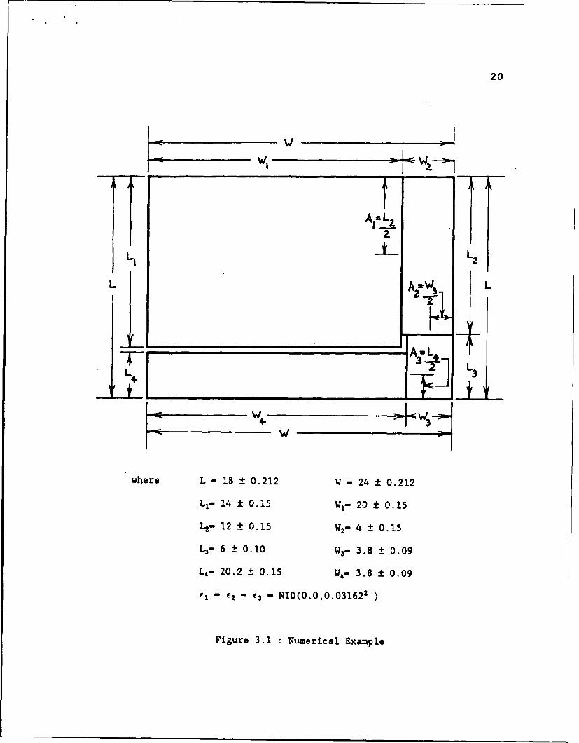
The numerical example used in this chapter is an assembly

consisting of four components that are assembled in three stages.

The geometry of the problem is given in Figure 3.1. Several

assumptions are used during the analysis of this problem. First, the

person or machine performing the assembly operation initially

determines the midpoint of the part to be joined to the base stage.

The assembler then finds the alignment point on the base stage. The

location of this alignment point is obtained using one-half of the

nominal for the part to be joined. The assembler then attempts to

join the two parts along these target lines. The assembler does this

task with a repeatability error, Ei for i - 1, 2, 3. The ci's are

assumed to be normally distributed with mean zero and variance ai2

Once the parts make contact, they are affixed to each other in some

manner (glue, weld, etc.). Finally, the manufacturing processes used

to manufacture the four components are also assumed to be normally

distributed with known mean and variance. The mean is assumed to be

equal to the nominal dimension of the part and the variance is

assumed to equal one-sixth of the total tolerance.

20

W

LI L

AwL

where L- 18 + 0.212 W - 24 ± 0.212

Lj- 14 ± 0.15 Wi- 20 ± 0.15

L2- 12 ± 0.15 W2- 4 0.15

L3- 6 + 0.10 W3- 3.8 ± 0.09

L4- 20.2 ± 0.15 W4- 3.8 ± 0.09

el- e2 3 - NID(0.0,0.031622 )

Figure 3.1 : Numerical Example

21

Determining the Expected

Number of Defectives

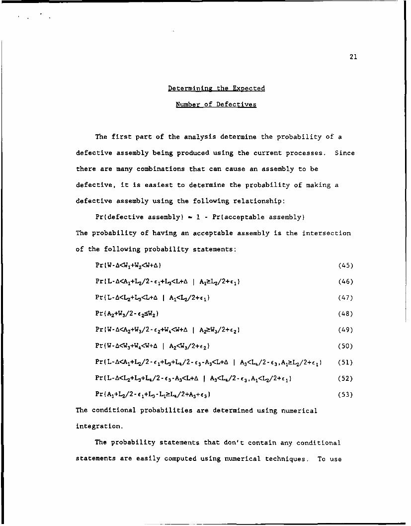
The first part of the analysis determine the probability of a

defective assembly being produced using the current processes. Since

there are many combinations that can cause an assembly to be

defective, it is easiest to determine the probability of making a

defective assembly using the following relationship:

Pr(defective assembly) - 1 - Pr(acceptable assembly)

The probability of having an acceptable assembly is the intersection

of the following probability statements:

Pr{W-A<W+W 2<W+A) (45)

Pr(L-A<AI+L2/2-ce+L 3<L+A I A1ZL2/2+,E) (46)

Pr { L-A<L2 +L3<L+A I A1<L2/2+el) (47)

Pr (A 2+W3/2 - C 2_<W 2 ) (48)

Pr(W-A<A2 +W3/2- e 2+W4<W+A I AZ>-W3/2+6 2 ) (49)

Pr(W-A< 3+W4<W+A I A 2<W 3/2+e 2 ) (50)

Pr(L-A<A+L 2/2-e,+L3+L4/2-e 3 -A3<L+A I A3<L4/2-C 3 ,Aj1 -L2/2+ej) (51)

Pr(L-A<L+L 3+L4/2-e 3-A3<L+A I A3<L4/2-C 3 ,A1 <L2/2+ej) (52)

Pr(A1+L2 /2- el+L 3-L LZL4/2+A3+e3) (53)

The conditional probabilities are determined using numerical

integration.

The probability statements that don't contain any conditional

statements are easily computed using numerical techniques. To use

22

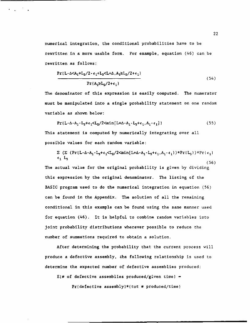
numerical integration, the conditional probabilities have to be

rewritten in a more usable form. For example, equation (46) can be

rewritten as follows:

Pr(L-A<A+L 2/2- 1+L3<L+A,Aj l2 /2+e1)(54)

Pr(Aj L2/2+e1 )

The denominator of this expression is easily computed. The numerator

must be manipulated into a single probability statement on one random

variable as shown below:

Pr{L-A-Al-L3+e,<L2/2<min[L+A-Al-L3+el,Al-l I] (55)

This statement is computed by numerically integrating over all

possible values for each random variable:

Z (Z (Pr(L-A-Al-L3+61<L2/2<min[L+A-Al-L3+61 ,Al-61 })*Pr(L3))*Pr{ e)

(56)The actual value for the original probability is given by dividing

this expression by the original denominator. The listing of the

BASIC program used to do the numerical integration in equation (56)

can be found in the Appendix. The solution of all the remaining

conditional in this example can be found using the same manner used

for equation (46). It is helpful to combine random variables into

joint probability distributions wherever possible to reduce the

number of summations required to obtain a solution.

After determining the probability that the current process will

produce a defective assembly, the following relationship is used to

determine the expected number of defective assemblies produced:

E(# of defective assemblies produced/given time) -

Pr(defective assembly)*(tot # produced/time)

23

For this example, the probability of a defective assembly is 0.02541

and the yearly production rate is 10,000 units. This yields 254.1

expected defective assemblies per year using the current processes.

Sensitivity Analysis

A sensitivity analysis performed on the assembly process in this

example is accomplished using the design of a complete 26 factorial

experiment. The six factors studied are the mean and variance for

the repeatability errors for each of the three assembly processes in

this example. The two levels for each mean are 0.01 and -0.01. The

two levels for each variance are 0.0004 and 0.0001. The results are

summarized in Table 3.1.

Table 3.1 : Sensitivity Analysis

factor effect - (Ehiah-Zlow)/64

Al -0.00195

/2 0.00011

IA3 -0.00183

a12 -0.00066

02 -0.00009

a32 -0.00087

From Table 3.1, it is clear that the first and third assembly

processes have the greatest effect on the probability of producing a

defective assembly. As may be expected, a change in the means has a

greater effect than a change in the variances.

24

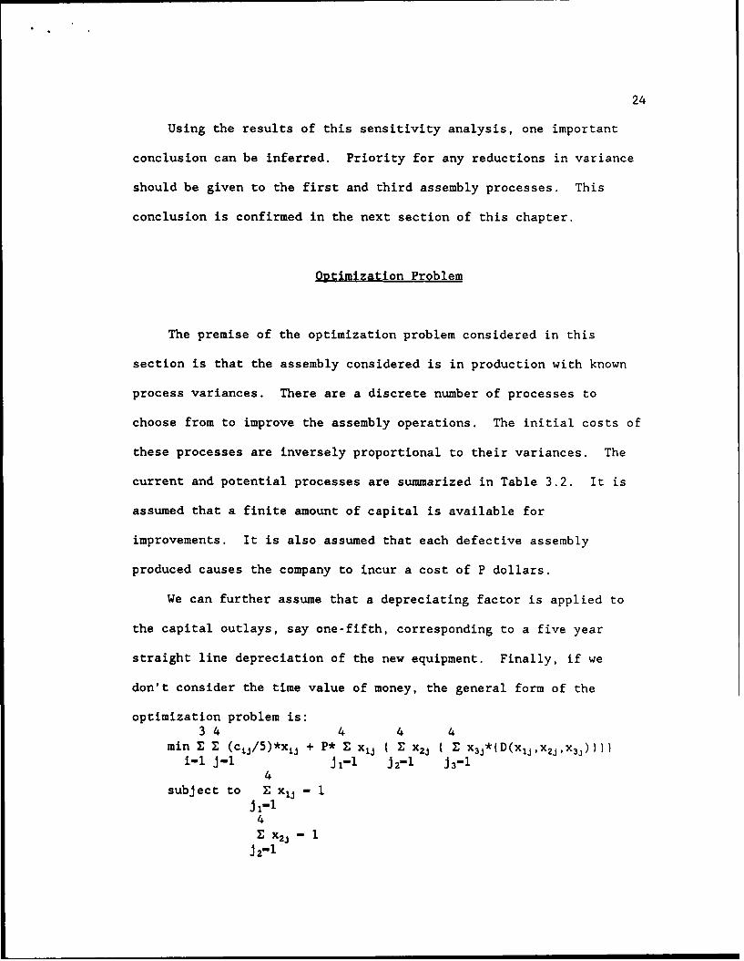
Using the results of this sensitivity analysis, one important

conclusion can be inferred. Priority for any reductions in variance

should be given to the first and third assembly processes. This

conclusion is confirmed in the next section of this chapter.

Optimization Problem

The premise of the optimization problem considered in this

section is that the assembly considered is in production with known

process variances. There are a discrete number of processes to

choose from to improve the assembly operations. The initial costs of

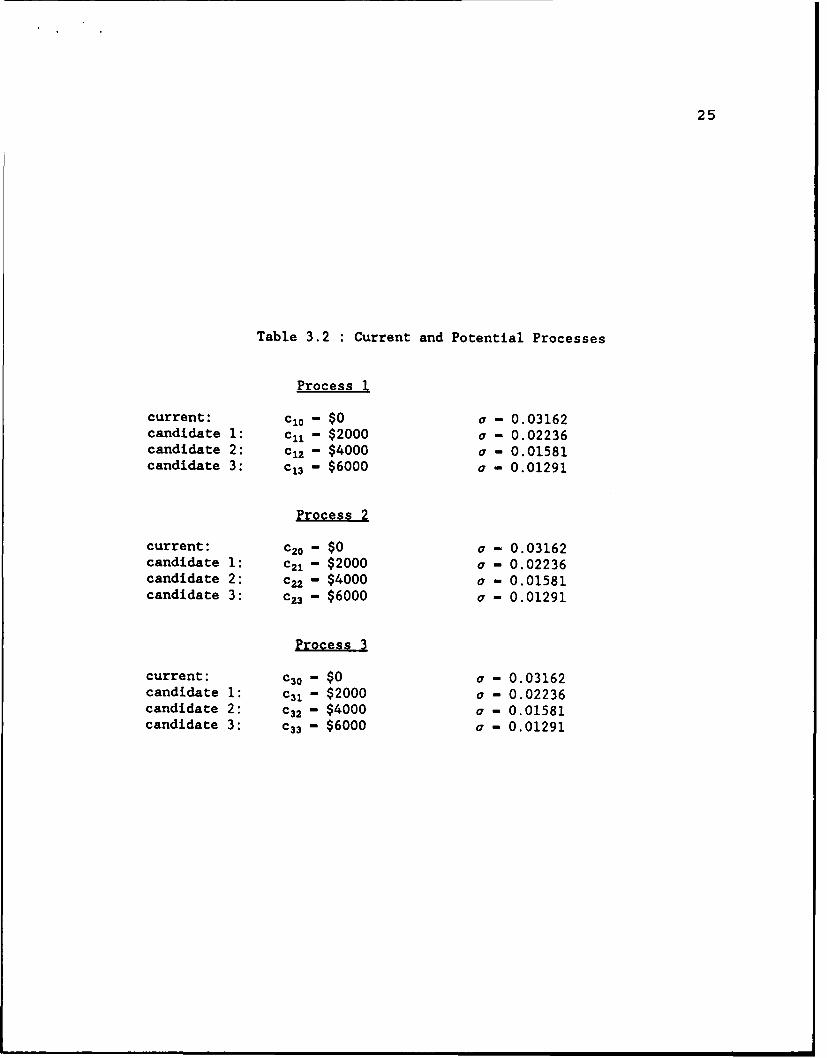
these processes are inversely proportional to their variances. The

current and potential processes are summarized in Table 3.2. It is

assumed that a finite amount of capital is available for

improvements. It is also assumed that each defective assembly

produced causes the company to incur a cost of P dollars.

We can further assume that a depreciating factor is applied to

the capital outlays, say one-fifth, corresponding to a five year

straight line depreciation of the new equipment. Finally, if we

don't consider the time value of money, the general form of the

optimization problem is:34 4 4 4

min E Z (cij/5)*xij + P* Z x 1j ( Z x2J ( Z x3j*(D(xljx 2Jx 3i))1

i-l J-1 ji-i j 2-1 j 3-i4

subject to Z x1-ji-1

4Z X2 j - 1

J 2-

25

Table 3.2 : Current and Potential Processes

Process 1

current: c10 - $0 a - 0.03162candidate 1: c11 - $2000 a - 0.02236candidate 2: c12 - $4000 a - 0.01581candidate 3: c13 - $6000 a - 0.01291

Process 2

current: c20 - $0 a - 0.03162candidate 1: c21 - $2000 a - 0.02236candidate 2: c22 - $4000 a - 0.01581candidate 3: c23 - $6000 a - 0.01291

Process3

current: c30 - $0 a - 0.03162candidate 1: c31 - $2000 a - 0.02236candidate 2: c32 - $4000 a - 0.01581candidate 3: c33 - $6000 a - 0.01291

26

4Z - 1J 3-1

3 4Z E cijxij _< investment amount

i-i j-i

1 if process j is selected at stage iXjj -

0 otherwise

This problem can be made into a straight integer programming problem

by introducing some constraints to ensure that one and only one

process is chosen as follows:

P*x 1 1 *x 2 1*x 3 1* (D (x 11 , x 2 1 , x 3 1 )

is rewritten as:

P*xd*(D(process combination d))

Xd Xll

Xd' X21

Xd'X31

xx 11 +x 21+x 31-2

The only drawback to this problem is that it requires total

enumeration of all of the possible expected number of defectives.

Although this sounds monumental, it is fairly easily done since the

basic probability statements are functions of one or two of the

assembly processes.

A parametric analysis of this problem is performed for several

levels of "defective costs" and investment capital. The results are

summarized in Table 3.3. The results of this analysis confirm the

sensitivity analysis performed earlier. It is optimal to reduce the

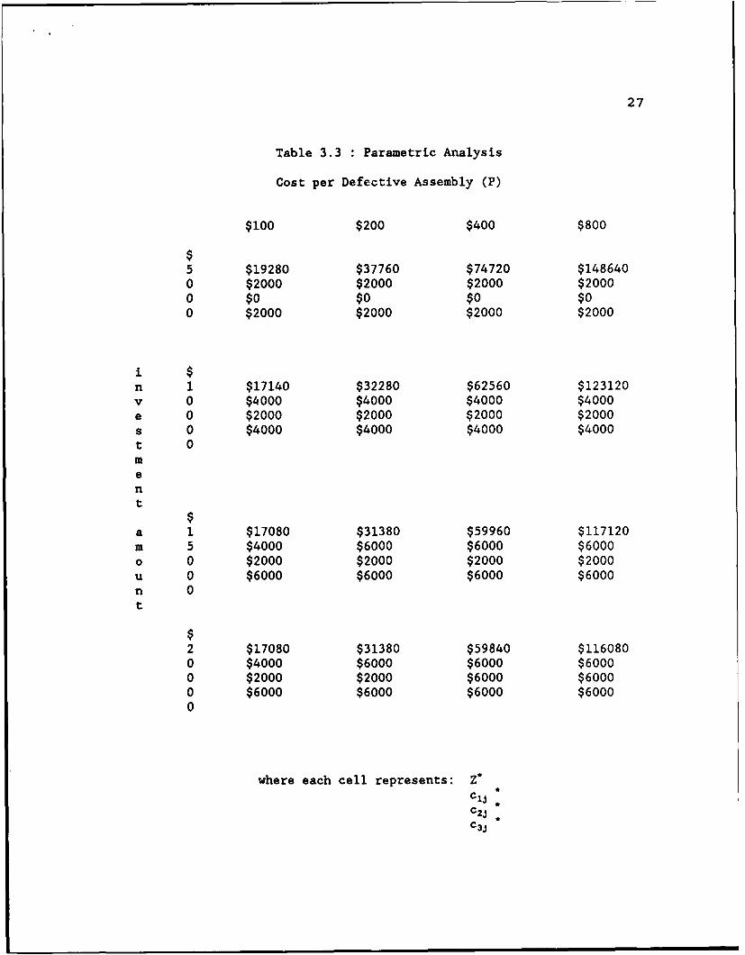
27

Table 3.3 : Parametric Analysis

Cost per Defective Assembly (P)

$100 $200 $400 $800

$5 $19280 $37760 $74720 $1486400 $2000 $2000 $2000 $20000 $0 $0 $0 $00 $2000 $2000 $2000 $2000

i $n 1 $17140 $32280 $62560 $123120v 0 $4000 $4000 $4000 $4000e 0 $2000 $2000 $2000 $2000s 0 $4000 $4000 $4000 $4000t 0ment $a 1 $17080 $31380 $59960 $117120m 5 $4000 $6000 $6000 $6000o 0 $2000 $2000 $2000 $2000u 0 $6000 $6000 $6000 $6000n 0t

$2 $17080 $31380 $59840 $1160800 $4000 $6000 $6000 $60000 $2000 $2000 $6000 $60000 $6000 $6000 $6000 $60000

where each cell represents: Z*

C2 j

C3j

28

variance of the first and third assembly processes before the second

process. It is also clear from this analysis that it may not be

advisable to expend all of the capital available for process

improvement, depending on the cost incurred per defective assembly.

This analysis could also be used to justify a request for increased

availability of capital improvement funds.

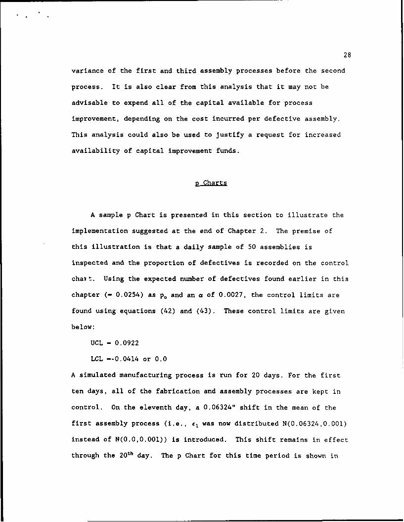
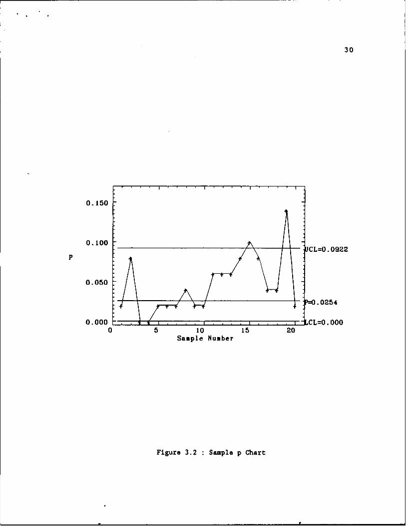
p Charts

A sample p Chart is presented in this section to illustrate the

implementation suggested at the end of Chapter 2. The premise of

this illustration is that a daily sample of 50 assemblies is

inspected and the proportion of defectives is recorded on the control

chait. Using the expected number of defectives found earlier in this

chapter (- 0.0254) as p. and an a of 0.0027, the control limits are

found using equations (42) and (43). These control limits are given

below:

UCL - 0.0922

LCL --0.0414 or 0.0

A simulated manufacturing process is run for 20 days. For the first

ten days, all of the fabrication and assembly processes are kept in

control. On the eleventh day, a 0.06324" shift in the mean of the

first assembly process (i.e., el was now distributed N(0.06324,0.001)

instead of N(0.0,0.001)) is introduced. This shift remains in effect

through the 2 0 th day. The p Chart for this time period is shown in

29

Figure 3.2. From Figure 3.2, this simulated process is detected as

being out of control on the 1 5th day. Once again, this result is not

unique, since each simulation run is different. This chart is

presented solely as an illustration of the method developed in this

paper.

30

0.150

0.100:CL=0 .0922

p

0.050.0

5

0.000 - CL=O. 0000 5 10 15 20

Sample Number

Figure 3.2 Sample p Chart

31

Chapter 4

CONCLUSIONS AND RECOMMENDATIONS

A method for analytically determining the acceptance

characteristics of a complex assembly process was developed. It was

shown that the basic relationships needed for this analysis were also

needed for the development of a simulation model, so this method did

not require much more effort from the analyst than that required for

a simulated result. The results of this analytic method were shown

to be very useful for optimally allocating limited capital

improvements and for assembly process control. An example problem

was presented that illustrated this analytic methodology as well as

the two applications that were developed.

There are many areas for further research in the area of

assembly process allocation and control. One possible area for

further research is the optimization problem. There may be some way

to formulate the problem in a continuous form that is solvable by

some nonlinear method. The problem can also be expanded to include

the fabrication processes as well as the assembly processes, thus

providing a more global optimization problem for a given system. The

objective function may include many more factors. For example, if a

candidate assembly process involves a piece of special tooling that

not only reduces assembly variance but is also more efficient for the

person doing the assembly, the reduced labor costs may be added to

32

the objective. Finally, the structure of the modified integer

programming problem is similar to a network type of problem. If the

constraint matrix can be manipulated to make the problem into a

network type of problem, a faster solution may be possible.

The Box-and-Cover problem also has many possibilities for

further research. If some of the random variables in this problem

can be combined to form joint distributions, the numerical

integrations in equations (38) and (40) may become feasible. This

eliminates the need for an approximate formulation of the problem.

Also, the possible forms for the approximate solution of thii problem

(i.e., using truncated distributions in the General assembly case)

can be further researched to provide more accurate results.

The final area for possible research is to expand this method to

electronic and electromechanical types of assemblies. Since purely

mechanical assemblies are only one small segment of industry today, a

method that can be used for different types of assembly processes can

be very useful. For example, the expected number of defectives for

an electronic assembly might possibly be used to predict the expected

yield of the assembly through an acceptance test procedure. This

expected yield can then be used to statistically control the assembly

process. This eliminates the need for arbitrary target levels for

acceptance yield that are commonly used, even though they have no

statistical basis. Management of assembly processes is more

effective when the foundation of that management is statistically

developed and analytically obtained. Management by arbitrary goals

33

and simulated results is always less than optimal.

One area for additional study is to develop a generalized

computer program that can handle a variable number of summations.

Ideally, the user is able to input the distribution parameters and

the limits of each sum interactively. The program should be written

in a compilable language to help speed the numerous calculations. In

addition, the program should minimize the number of times that the

normal probability subroutine is called from within a summation.

This can be accomplished through a clever use of arrays. The program

in the Appendix is written in BASIC since every computer has some

form of BASIC available with the initial software.

34

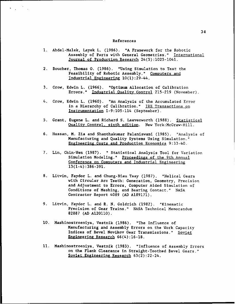
References

1. Abdel-Malek, Layek L. (1986). "A Framework for the RoboticAssembly of Parts with General Geometries." InternationalJournal of Production Research 24(5):1025-1041.

2. Boucher, Thomas 0. (1986). "Using Simulation to Test theFeasibility of Robotic Assembly." Computers andIndustrial Engineering 10(1):29-44.

3. Crow, Edwin L. (1966). "Optimum Allocation of CalibrationErrors." Industrial Quality Control 215-219 (November).

4. Crow, Edwin L. (1960). "An Analysis of the Accumulated Errorin a Hierarchy of Calibration." IRE Transactions onInstrumentation 1-9:105-114 (September).

5. Grant, Eugene L. and Richard S. Leavenworth (1988). StatisticalQuality Control. sixth edition. New York:McGraw-Hill.

6. Hassan, M. Zia and Shanthakumar Palaniswami (1985). "Analysis ofManufacturing and Quality Systems Using Simulation."Engineering Costs and Production Economics 9:33-40.

7. Lin, Chin-Wen (1987). " Statistical Analysis Tool for VariationSimulation Modeling." Proceedings of the 9th AnnualConference on Computers and Industrial Engineering13(1-4):386-391.

8. Litvin, Faydor L. and Chung-Biau Tsay (1987). "Helical Gearswith Circular Arc Teeth: Generation, Geometry, Precisionand Adjustment to Errors, Computer Aided Simulation ofConditions of Meshing, and Bearing Contact." NASAContractor Report 4089 (AD A189171).

9. Litvin, Faydor L. and R. N. Goldrich (1982). "KinematicPrecision of Gear Trains." NASA Technical Memorandum82887 (AD A120110).

10. Mashinostroeniya, Vestnik (1986). "The Influence ofManufacturing and Assembly Errors on the Work CapacityIndices of Bevel Novikov Gear Transmissions." SovietEngineering Research 66(4):16-18.

11. Mashinostroeniya, Vestnik (1983). "Influence of Assembly Errorson the Flank Clearance in Straight-Toothed Bevel Gears."Soviet Engineering Research 63(2):22-24.

35

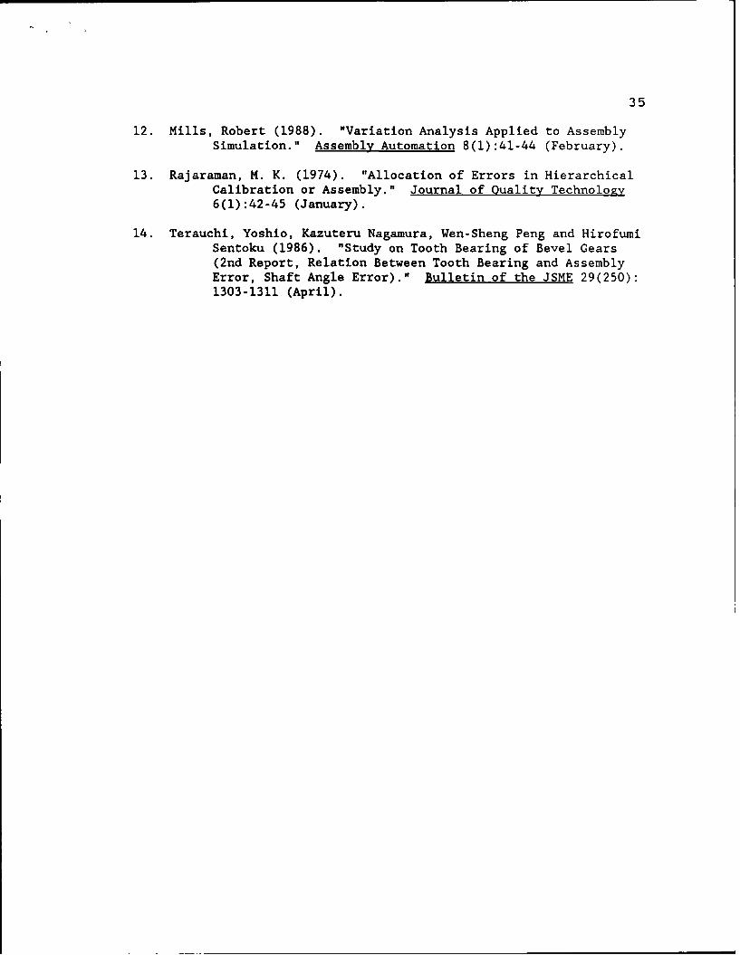
12. Mills, Robert (1988). "Variation Analysis Applied to AssemblySimulation." Assembly Automation 8(1):41-44 (February).

13. Rajaraman, M. K. (1974). "Allocation of Errors in HierarchicalCalibration or Assembly." Journal of Quality Technology6(l):42-45 (January).

14. Terauchi, Yoshio, Kazuteru Nagamura, Wen-Sheng Peng and HirofumiSentoku (1986). "Study on Tooth Bearing of Bevel Gears(2nd Report, Relation Between Tooth Bearing and AssemblyError, Shaft Angle Error)." Bulletin of the JSME 29(250):1303-1311 (April).

4

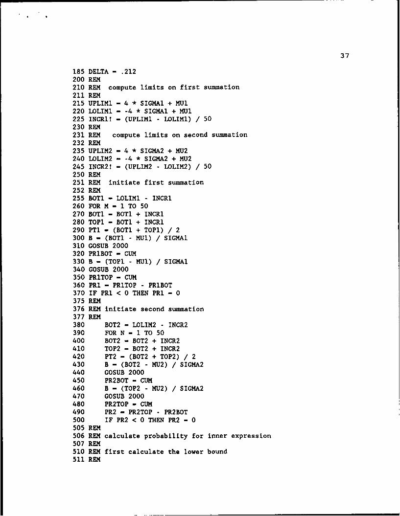
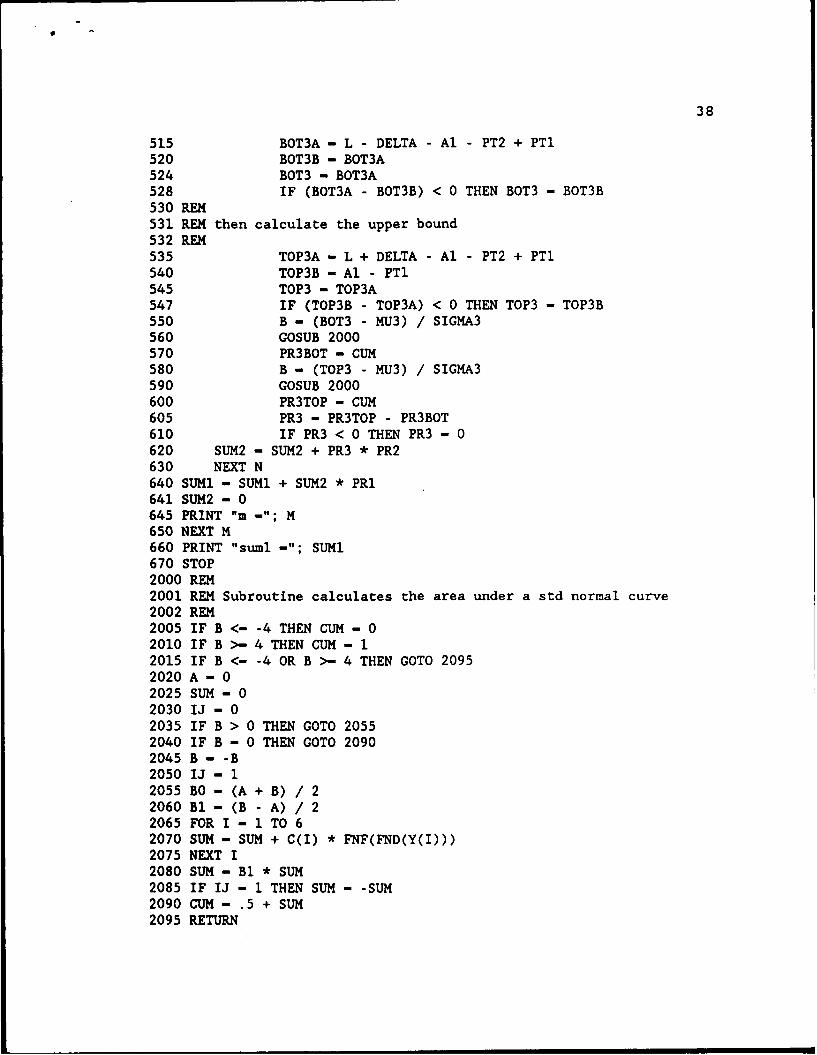
36

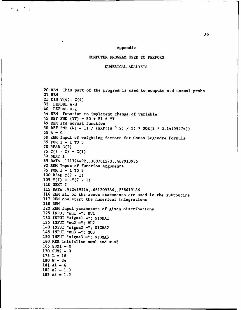
Appendix

COMPUTER PROGRAM USED TO PERFORM

NUMERICAL ANALYSIS

20 REM This part of the program is used to compute std normal probs21 REM25 DIM Y(6), C(6)35 DEFDBL A-H40 DEFDBL O-Z44 REM Function to implement change of variable45 DEF FND (YT) - BO + Bi * YT49 REM std normal function50 DEF FNF (W) - 1! / (EXP((W A 2) / 2) * SQR(2 * 3.1415927#))55 A - 060 REM Input of weighting factors for Gauss-Legendre Formula65 FOR I - 1 TO 370 READ C(I)75 C(7 - I) - C(I)80 NEXT I85 DATA .171324492,.360761573,.46791393590 REM Input of function arguments95 FOR I - 1 TO 3100 READ Y(7 - I)105 Y(I) - -Y(7 - I)110 NEXT I115 DATA .932469514,.661209386,.238619186116 REM all of the above statements are used in the subroutine117 REM now start the numerical integrations118 REM120 REM input parameters of given distributions125 INPUT "mul -"; MUl130 INPUT "sigmal -"; SIGMAl135 INPUT "mu2 -"; MU2140 INPUT "sigma2 -"; SIGMA2145 INPUT "mu3 -"; MU3150 INPUT "sigma3 -"; SIGMA3160 REM initialise sumi and sum2165 SUM1 - 0170 SUM2 - 0175 L - 18180 W - 24181 Al - 6182 A2 - 1.9183 A3 - 1.9

37

185 DELTA - .212200 REM210 REM compute limits on first summation211 REM215 UPLIMI - 4 * SIGMAl + MUl220 LOLIMI - -4 * SIGMAl + MUI225 INCRI! - (UPLIMi - LOLIMI) / 50230 REM231 REM compute limits on second summation232 REM235 UPLIM2 - 4 * SIGMA2 + MU2240 LOLIM2 - -4 * SIGMA2 + MU2245 INCR2! - (UPLIM2 - LOLIM2) / 50250 REM251 REM initiate first summation252 REM255 BOTI - LOLIMI - INCRI260 FOR M - 1 TO 50270 BOTI - BOTi + INCRI280 TOPI - BOTI + INCRI290 PT1 - (BOTI + TOP1) / 2300 B - (BOTI - MUl) / SIGMAl310 GOSUB 2000320 PRIBOT - CUM330 B - (TOPI - MUI) / SIGMAl340 GOSUB 2000350 PRITOP - CUM360 PR1 - PRITOP - PRIBOT370 IF PRI < 0 THEN PRI - 0375 REM376 REM initiate second summation377 REM380 BOT2 - LOLIM2 - INCR2390 FOR N - I TO 50400 BOT2 - BOT2 + INCR2410 TOP2 - BOT2 + INCR2420 PT2 - (BOT2 + TOP2) / 2430 B - (BOT2 - MU2) / SIGMA2440 GOSUB 2000450 PR2BOT - CUM460 B - (TOP2 - MU2) / SIGMA2470 GOSUB 2000480 PR2TOP - CUM490 PR2 - PR2TOP - PR2BOT500 IF PR2 < 0 THEN PR2 - 0505 REM506 REM calculate probability for inner expression507 REM510 REM first calculate the lower bound511 REM

38

515 BOT3A - L - DELTA - Al - PT2 + PT1520 BOT3B - BOT3A524 BOT3 - BOT3A528 IF (BOT3A - BOT3B) < 0 THEN BOT3 - BOT3B530 REM531 REM then calculate the upper bound532 REM535 TOP3A - L + DELTA - Al - PT2 + PTI540 TOP3B - Al - PTl545 TOP3 - TOP3A547 IF (TOP3B - TOP3A) < 0 THEN TOP3 - TOP3B550 B - (BOT3 - MU3) / SIGMA3560 GOSUB 2000570 PR3BOT - CUM580 B - (TOP3 - MU3) / SIGMA3590 GOSUB 2000600 PR3TOP - CUM605 PR3 - PR3TOP - PR3BOT610 IF PR3 < 0 THEN PR3 - 0620 SUM2 - SUM2 + PR3 * PR2630 NEXT N640 SUM1 - SUM1 + SUM2 * PRI641 SUM2 - 0645 PRINT "m-"; M650 NEXT M660 PRINT "suml -"; SUM1670 STOP2000 REM2001 REM Subroutine calculates the area under a std normal curve2002 REM2005 IF B <- -4 THEN CUM - 02010 IF B >- 4 THEN CUM - 12015 IF B <- -4 OR B >- 4 THEN GOTO 20952020 A - 02025 SUM - 02030 IJ - 02035 IF B > 0 THEN GOTO 20552040 IF B - 0 THEN GOTO 20902045 B- -B2050 IJ - 12055 BO - (A + B) / 22060 Bi - (B - A) / 22065 FOR I - 1 TO 62070 SUM - SUM + C(I) * FNF(FND(Y(I)))2075 NEXT I2080 SUM - Bl * SUM2085 IF IJ - 1 THEN SUM - -SUM2090 CUM - .5 + SUM2095 RETURN