Embed Size (px)
Citation preview

Modelling global greeninvestment scenarios
Version 02.11.2011
Supporting the transition to a global green economy
Towards a green economy
Acknowledgements Chapter Coordinating Author: Dr Andrea M. Bassi, Deputy Director, Project Development and Modelling, Millennium Institute, USA, with support from John P. Ansah and Zhuohua Tan, Millennium Institute.
Contributing Author: Matteo Pedercini, Millennium Institute.
Derek Eaton and Sheng Fulai (in the initial stages of the project) of UNEP managed the chapter, including the elaboration of modelling scenarios, the handling of peer reviews, interacting with the coordinating authors on revisions, conducting supplementary research and bringing the chapter to final production.
Peter Poschen and numerous colleagues at the International Labour Organization (ILO), including among others, Ekkehard Ernst and Mathieu Charpe, contributed substantially with insights, data and critique, particularly on employment-related aspects. Ana Lucía Iturriza provided support to the chapter managers and coordinated ILO’s contributions.
The following members of chapter author teams contributed to the refinement of the model and provided feedback on results: Bob Ayres, Amos Bien, Holger Dalkmann, Maryanne Grieg-Gran, Hans Herren, Andreas Koch, Cornis van der Lugt, Prasad Modak, Lawrence Pratt, Luis Rivera, Philipp Rode, Ko Sakamoto, Rashid Sumaila, Arnold Tukker, Xander van Tilburg, Peter Wooders; and Mike D. Young.
During the development of the modelling analysis, the Chapter Coordinating Author received invaluable advice and inputs from the following: Alan AtKisson (AtKisson Group, Sweden); Laura Cozzi (International Energy Agency); Paal Davidsen and Erling Moxnes (University of Bergen, Norway);
Prakash (Sanju) Deenapanray (Ecological Living in Action); Prakash (Sanju) Deenapanray (Ecological Living in Action); Alan Drake (USA); Jospeh Fiksel and Emrah Cimren (Ohio State University, USA); Michael Goodsite (National Environmental Research Institute, Denmark); Cornis van der Lugt (UNEP); Desta Mebratu (UNEP); Donatella Pasqualini (Los Alamos National Laboratory USA); Mark Radka (UNEP); Kenneth Ruffing (Consultant); Guido Sonnemann (UNEP); Serban Srieciu (UNEP); William Stafford (Council for Scientific Industrial Research, South Africa); Niclas Svenningsen (UNEP); Mathis Wackernagel (Global Footprint Network); Jaap van Woerden (UNEP GRID); and Joel Yudken (High Road Strategies, USA).
We would like to thank those who provided detailed comments on the review draft, including Santiago Arango Aramburo (National University of Colombia); Simon Buckle (Grantham Institute for Climate Change, Imperial College London, UK); Jean Chateau (Organisation for Economic Co-operation and Development); Jeanneney Guillaumont (CERDI, University of Auvergne, France); Li Shantong (Development Research Center, State Council, China); Peter Poschen (International Labour Organization); Mohamed Saleh (Cairo University, Egypt); and Stefan Speck (European Environment Agency).
We would also like to thank individuals and organizations who offered comments on the advance copy, including Tim Jackson (University of Surrey, UK); Peter Victor (York University, Canada); the Bureau of Economic Analysis of the US Department of Commerce; the Global Footprint Network; Novozymes; and the United Nations Fund for Population Activities (UNFPA).
Copyright © United Nations Environment Programme, 2011Version -- 02.11.2011
498
ContentsList of acronyms . . . . . . . . . . . . . . . . . . . . . . . . . . . . . . . . . . . . . . . . . . . . . . . . . . . . . . . . . . . . . . . . . . . 503
Key messages. . . . . . . . . . . . . . . . . . . . . . . . . . . . . . . . . . . . . . . . . . . . . . . . . . . . . . . . . . . . . . . . . . . . . . 504
1 Introduction. . . . . . . . . . . . . . . . . . . . . . . . . . . . . . . . . . . . . . . . . . . . . . . . . . . . . . . . . . . . . . . . . . 506
2 Understanding the green economy . . . . . . . . . . . . . . . . . . . . . . . . . . . . . . . . . . . . . . . . . . . . 507
3 Modelling the green economy . . . . . . . . . . . . . . . . . . . . . . . . . . . . . . . . . . . . . . . . . . . . . . . . . 5093.1 A characterisation of modelling approaches. . . . . . . . . . . . . . . . . . . . . . . . . . . . . . . . . . . . . . . . . . . . . . . . . . . 5093.2 The Threshold 21 World model. . . . . . . . . . . . . . . . . . . . . . . . . . . . . . . . . . . . . . . . . . . . . . . . . . . . . . . . . . . . . . . . 509
4 Scenario definition and challenges. . . . . . . . . . . . . . . . . . . . . . . . . . . . . . . . . . . . . . . . . . . . . 5114.1 Defining investments and methodology . . . . . . . . . . . . . . . . . . . . . . . . . . . . . . . . . . . . . . . . . . . . . . . . . . . . . . 513
5 Results of the simulations and analysis . . . . . . . . . . . . . . . . . . . . . . . . . . . . . . . . . . . . . . . . . 5155.1 Baseline projection (BAU) . . . . . . . . . . . . . . . . . . . . . . . . . . . . . . . . . . . . . . . . . . . . . . . . . . . . . . . . . . . . . . . . . . . . . 5155.2 Green economy projections . . . . . . . . . . . . . . . . . . . . . . . . . . . . . . . . . . . . . . . . . . . . . . . . . . . . . . . . . . . . . . . . . . 518
6 Conclusions . . . . . . . . . . . . . . . . . . . . . . . . . . . . . . . . . . . . . . . . . . . . . . . . . . . . . . . . . . . . . . . . . . 533
Annex 1. Technical specifications of the Threshold 21 (T21) World model . . . . . . . . . . . . . . 537
References . . . . . . . . . . . . . . . . . . . . . . . . . . . . . . . . . . . . . . . . . . . . . . . . . . . . . . . . . . . . . . . . . . . . . . . . 541
Modelling
499
Towards a green economy
List of figuresFigure 1: The relations between economic growth and natural resources . . . . . . . . . . . . . . . . . . . . . . . . . . . . . 507 Figure 2: Conceptual overview of T21-World . . . . . . . . . . . . . . . . . . . . . . . . . . . . . . . . . . . . . . . . . . . . . . . . . . . . . . . . . 510Figure 3: Representation of the main underlying assumptions of green and BAU investments . . . . . . . . . 512Figure 4: Simulation of population in BAU compared with population values of WPP. . . . . . . . . . . . . . . . . . 515Figure 5: Simulation of total volume of crop yield in BAU compared with values of FAOSTAT. . . . . . . . . . . 515Figure 6: Simulation of oil demand in BAU compared with values of WEO*. . . . . . . . . . . . . . . . . . . . . . . . . . . . 516Figure 7: Simulation of arable land and forestland in BAU compared with values of FAOSTAT . . . . . . . . . . 516Figure 8 and Figure 9: Simulation of fossil-fuel CO2 emissions in BAU compared with WEO values; Simulation of footprint/biocapacity in BAU compared with values of Global Footprint Network . . . . . . . 517Figure 10: Results of the G1 scenario relative to the BAU1 case in 2015, 2030 and 2050 (per cent) . . . . . . 519Figure 11: Results of the G2 scenario in 2015, 2030 and 2050 relative to BAU2 (per cent) . . . . . . . . . . . . . . 519
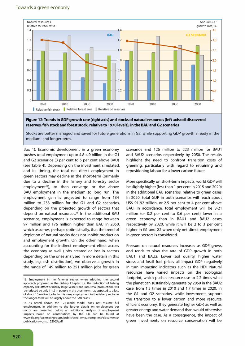
Figure 12: Trends in GDP growth rate (right axis) and stocks of natural resources (left axis: oil discovered reserves, fish stock and forest stock, relative to 1970 levels), in the BAU and G2 scenarios . . 520Figure 13: Trends in annual GDP growth rate, historical data (WDI, 2009) and projections in BAU, BAU2 and G2 scenarios . . . . . . . . . . . . . . . . . . . . . . . . . . . . . . . . . . . . . . . . . . . . . . . . . . . . . . . . . . . . . . . . . . . . . . . . 523Figure 14: Fossil fuel CO2 emissions in additional BAU and green scenarios relative to the BAU case. . . . 524Figure 15: Composition of ecological footprint in 2050 in various scenarios, relative to 1970 value and indication of the projected footprint-biocapacity ratio in 2050 . . . . . . . . . . . . . . . . . . . . . . . . . . . . 524
Figure 16: Causal loop diagram (CLD) representing the main factors influencing crop yield in the agriculture sector of the model . . . . . . . . . . . . . . . . . . . . . . . . . . . . . . . . . . . . . . . . . . . . . . . . . . . . . . . . . . . . . . . . . . . . . 525Figure 17: Land allocation in 2050 under BAU and the G2 scenario, in billion hectares and as a share of total land . . . . . . . . . . . . . . . . . . . . . . . . . . . . . . . . . . . . . . . . . . . . . . . . . . . . . . . . . . . . . . . . . . . . . . . . . . . . . . . . 526Figure 18: Total forest stocks and flows of deforestation and reforestation in BAU, BAU2 and G2 scenarios . . . . . . . . . . . . . . . . . . . . . . . . . . . . . . . . . . . . . . . . . . . . . . . . . . . . . . . . . . . . . . . . . . . . . . . . . . . . . . . . . . . . . . . 526Figure 19: Fish stock relative to 1970 level and fish catch in BAU, BAU2 and G2 scenarios . . . . . . . . . . . . . . 527Figure 20: Results of the sensitivity analysis for (a) fish stock relative to 1970 level and (b) fish catch in tonnes/year. . . . . . . . . . . . . . . . . . . . . . . . . . . . . . . . . . . . . . . . . . . . . . . . . . . . . . . . . . . . . . . . . . . . . . . . . 527Figure 21: Global conventional oil production scenarios considered in the GER . . . . . . . . . . . . . . . . . . . . . . . 528Figure 22: Trends in BAU and G2 scenarios (a) in total energy consumption and renewable penetration rate (right axis), (b) power generation and renewable penetration rate in power sector . . . 529Figure 23: Composition of power supply employment in 2050 in various scenarios in power plants (in manufacturing, construction, installation and operation and management), power supply fuels, energy efficiency . . . . . . . . . . . . . . . . . . . . . . . . . . . . . . . . . . . . . . . . . . . . . . . . . . . . . . . . . . . . . . . . . . . . . . . . . . . . . . . . . . . 530Figure 24: Total employment in the energy sector, and its disaggregation into fuel and power, and energy efficiency . . . . . . . . . . . . . . . . . . . . . . . . . . . . . . . . . . . . . . . . . . . . . . . . . . . . . . . . . . . . . . . . . . . . . . . . . . . . . . . . . . . 531Figure 25: Water supply by source and water demand by sector (km3), under BAU baseline and G2 scenarios . . . . . . . . . . . . . . . . . . . . . . . . . . . . . . . . . . . . . . . . . . . . . . . . . . . . . . . . . . . . . . . . . . . . . . . . . . . . . . . . . . . . . . . 532Figure A1: Spheres and sectors of T21-World. . . . . . . . . . . . . . . . . . . . . . . . . . . . . . . . . . . . . . . . . . . . . . . . . . . . . . . . . 538
500
Modelling
List of tablesTable 1: Comparison of scenarios for selected sectors and objectives . . . . . . . . . . . . . . . . . . . . . . . . . . . . . . . . . 512Table 2: Allocation of investments across sectors in the G1 and G2 scenarios as a share of total investment and GDP (2011 – 2050 average) and sectoral targets of green scenarios . . . . . . . . . . . . . . . . . . 513Table 3: Transport emissions by mode in business-as-usual scenarios of GER and IEA. . . . . . . . . . . . . . . . . . 517Table 4: Main indicators, BAU and green investment scenarios . . . . . . . . . . . . . . . . . . . . . . . . . . . . . . . . . . . . . . . 518Table 5: Comparison of energy mix in 2030 and 2050 in various GER and IEA scenarios . . . . . . . . . . . . . . . . 529Table 6: Transport energy consumption in green scenarios of GER and IEA, in selected years . . . . . . . . . . 531Table 7: Main indicators in BAU and green investment scenarios . . . . . . . . . . . . . . . . . . . . . . . . . . . . . . . . . . . . . 534Table 8: Comparison (per cent) of main indicators in G1 scenario relative to BAU1 scenario (1 per cent case) and G2 scenario relative to BAU2 scenario (2 per cent case). . . . . . . . . . . . . . . . . . . . . . . . . . 536
List of boxesBox 1: Changes in natural capital stocks . . . . . . . . . . . . . . . . . . . . . . . . . . . . . . . . . . . . . . . . . . . . . . . . . . . . . . . . . . . . . 522Box A1: The Cobb-Douglas production function in T21 for agriculture, industry and services macro sectors . . . . . . . . . . . . . . . . . . . . . . . . . . . . . . . . . . . . . . . . . . . . . . . . . . . . . . . . . . . . . . . . . . . . . . . . . . . . . . 539
501

Towards a green economy
502
Modelling
List of acronyms
AR4 Fourth Assessment Report of the IPCCBAU Business-as-usualCCS Carbon capture and storageCD Cobb-Douglas CGE Computable General Equilibrium CLD Causal loop diagramCO2-eq Carbon dioxide equivalentDC Disaggregated Consistency ETP Energy Technology PerspectivesFAO Food and Agricultural Organization of the United NationsFAOSTAT Food and Agriculture Organization Statistical DatabaseGDP Gross Domestic ProductGER Green Economy ReportGFN Global Footprint NetworkGGND Global Green New DealGHG Greenhouse gasHDI Human Development IndexIEA International Energy AgencyIIASA International Institute for Applied Systems AnalysisILO International Labour OrganizationIPCC Intergovernmental Panel on Climate ChangeLge Litres of gasoline equivalentMDGs Millennium Development GoalsME Macro-Econometric MoMo Mobility Model (Transport Model of IEA)Mtoe Million tonnes of oil equivalentNDP Net Domestic ProductO&M Operations and maintenanceOECD Organisation for Economic Co-operation and DevelopmentR&D Research and developmentRE Renewable energyROI Return on investmentSD System DynamicsT21 Threshold 21 modelTFP Total factor productivityUNEP United Nations Environment ProgrammeWDI World Development IndicatorsWEO World Energy OutlookWPP World Population Prospect
503
Towards a green economy
Key messages1. A Green Economy grows faster than a brown economy over time, while maintaining and restoring natural capital. Quantitative modelling for the Green Economy Report demonstrates that greening can not only generate increases in natural capital, but also produce a higher rate of Gross Domestic Product (GDP) growth – a classical, if outdated, measure of economic performance. Gross Domestic Product in the green scenario is projected to overtake business-as-usual (BAU) within ten years. An adjusted measure of net domestic product, accounting for both physical capital depreciation and also for natural capital depletion, achieves this result even earlier, indicating that a green economy offers improved and integrated capital management.
2. Business-as-usual can only deliver development gains at an unaffordable price. Under a BAU scenario, which replicates historical trends and assumes no fundamental changes in policy or external conditions to alter the trends, development benefits in terms of GDP growth and poverty reduction may continue for some time. But, these development gains would be achieved at an unaffordable price. Business-as-usual continues on the current high carbon intensity development path, with its associated environmental impacts, especially in terms of the long-term concentration of atmospheric greenhouse gases (GHG), which would approximate 1,000 ppm CO2-eq by 2100, resulting in temperature increases most likely around 4 degrees centigrade (as per IPCC scenarios A1B and A2). In addition, BAU would also significantly draw down natural capital assets; the results indicate that the global ecological footprint would be more than two times the available bio-capacity of the earth.
3. A green economy promotes pro-poor growth and achieves energy and resource efficiency. A green economy strengthens pro-poor economic growth through building up natural capital, on which the livelihood of the poor depends. In a green investment scenario, 2 per cent of global GDP is allocated to greening the energy, manufacturing, transport, buildings, waste, agriculture, fisheries, water and forests sectors. In the simulations, these investments help to, by 2050, potentially double fish stocks, and increase forestland by one-fifth, as compared to BAU. They would also reduce use of fossil fuels by 40 per cent, and demand for water by about 20 per cent, relative to BAU. By maintaining and building up natural capital and mitigating resource scarcity, these investments would provide the basis for enhanced human well-being, and sustained economic growth over the next 20 to 40 years, at least as strong as BAU with considerably reduced downside risks.
504
Modelling
4. A green economy has the potential to create additional jobs in the medium to long run. A shift to a green economy also means a shift in employment, which, at a minimum, should not lead to a net loss of jobs. The jobs created will at least make up for the losses that would be incurred from transforming environmentally unsustainable activities. In the short- and medium-term, the net direct employment under green investment scenarios may decline due to the need to reduce excessive resource extraction in sectors such as fisheries. But between 2030 and 2050, these green investments would create employment gains to catch up with and likely exceed BAU, under which employment growth will be further constrained by resource and energy scarcity and the impact of climate change.
5. The greening of most economic sectors would reduce GHG emissions significantly. With about 1.25 per cent of global GDP invested in raising energy efficiency across sectors and expanding renewable energy, including second generation biofuels, global energy intensity would be reduced by 36 per cent by 2030 and annual volume of energy-related CO2 emissions would decline to 20 Gt in 2050 from 30.6 Gt in 2010. Including the potential carbon sequestration of green agriculture, a green investment scenario is expected to reduce the concentration of emissions to 450 ppm by 2050, a level essential for having a reasonable likelihood of limiting global warming to the threshold of 2 degrees centigrade.
6. A green economy sustains and enhances ecosystem services. Green investments in the forestry and agricultural sectors would help reverse the current declines in forestland, rejuvenating this important resource to about 4.5 billion hectares over the next 40 years. Higher yields from investing in green agriculture would reduce the amount of land used for crops and livestock in 2050 by 6 per cent compared with projected BAU trends, while producing more food. Soil quality would rise by a quarter on average in 40 years. In addition, investments to increase water supply and expand access, while improving management, would provide an additional 10 per cent of global water supply in both the short- and long-term, and also contribute to sustaining groundwater and surface water resources. In the fisheries sector, the reduction of excessive capacity would help fish stocks to recover by 2050 to 70 per cent of their total level in 1970, as compared with a projected further decline to 30 per cent of the 1970 level under BAU. These investments in “ecological infrastructure” help to restore the earth’s bio-capacity and also to enhance human well-being.
505
Towards a green economy
1 Introduction
This chapter describes the modelling exercise conducted for the entire Green Economy Report (GER) and presents its results. The modelling was to test the hypothesis – which gave rise to this report – that investing in the environment delivers positive macroeconomic results, in addition to improving the environment. The modelling tool used is the Threshold 21 World model (T21-World), which comprises several sectoral models integrated into a global model. The sectoral models are at the core of the modelling exercise supporting the analysis carried out by the authors of the GER. The modelling traces the effects of investing various amounts of GDP in green – as opposed to business-as-usual (BAU) – economic activities in terms of stimulating the economy, improving resource efficiency, lowering carbon intensity, and creating jobs.
The next section describes the key issues that need to be addressed by a modelling framework that tries to quantify the challenges of moving towards a green economy. The third section describes key features of the modelling structure. This is followed by a section describing the assumptions underlying the various scenarios: a BAU scenario with no additional
investment, two BAU scenarios with increased levels of investment, but no change in energy and environmental policies (BAU1 and BAU2), and two green scenarios which combine the higher levels of investment with improved environmental polices (G1 and G2). After that, a fifth section describes the results of the various scenarios. This is followed by a short concluding section. Additional technical details are provided in an Annex as well as in the separate Technical Background Material.
It should be noted that all sector chapters in this report have, to a varying extent, made use of the results from the modelling exercise presented here. Although the modelling includes a number of scenarios, the sector chapters generally compare only one green scenario, G2, with the corresponding BAU2 scenario, in addition to describing relevant aspects of the baseline BAU scenario. The G2 scenario is more relevant as it explicitly aims to reduce CO2 emissions sufficiently to achieve an atmospheric concentration of 450 ppm, as well as a number of other policy targets in the areas of nutrition, fisheries management, reducing deforestation, water availability and waste management.
506
Modelling
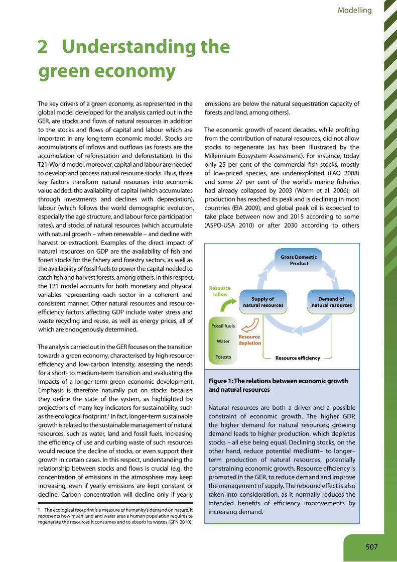
2 Understanding the green economyThe key drivers of a green economy, as represented in the global model developed for the analysis carried out in the GER, are stocks and flows of natural resources in addition to the stocks and flows of capital and labour which are important in any long-term economic model. Stocks are accumulations of inflows and outflows (as forests are the accumulation of reforestation and deforestation). In the T21-World model, moreover, capital and labour are needed to develop and process natural resource stocks. Thus, three key factors transform natural resources into economic value added: the availability of capital (which accumulates through investments and declines with depreciation), labour (which follows the world demographic evolution, especially the age structure, and labour force participation rates), and stocks of natural resources (which accumulate with natural growth – when renewable – and decline with harvest or extraction). Examples of the direct impact of natural resources on GDP are the availability of fish and forest stocks for the fishery and forestry sectors, as well as the availability of fossil fuels to power the capital needed to catch fish and harvest forests, among others. In this respect, the T21 model accounts for both monetary and physical variables representing each sector in a coherent and consistent manner. Other natural resources and resource-efficiency factors affecting GDP include water stress and waste recycling and reuse, as well as energy prices, all of which are endogenously determined.
The analysis carried out in the GER focuses on the transition towards a green economy, characterised by high resource-efficiency and low-carbon intensity, assessing the needs for a short- to medium-term transition and evaluating the impacts of a longer-term green economic development. Emphasis is therefore naturally put on stocks because they define the state of the system, as highlighted by projections of many key indicators for sustainability, such as the ecological footprint.1 In fact, longer-term sustainable growth is related to the sustainable management of natural resources, such as water, land and fossil fuels. Increasing the efficiency of use and curbing waste of such resources would reduce the decline of stocks, or even support their growth in certain cases. In this respect, understanding the relationship between stocks and flows is crucial (e.g. the concentration of emissions in the atmosphere may keep increasing, even if yearly emissions are kept constant or decline. Carbon concentration will decline only if yearly
1. The ecological footprint is a measure of humanity’s demand on nature. It represents how much land and water area a human population requires to regenerate the resources it consumes and to absorb its wastes (GFN 2010).
emissions are below the natural sequestration capacity of forests and land, among others).
The economic growth of recent decades, while profiting from the contribution of natural resources, did not allow stocks to regenerate (as has been illustrated by the Millennium Ecosystem Assessment). For instance, today only 25 per cent of the commercial fish stocks, mostly of low-priced species, are underexploited (FAO 2008) and some 27 per cent of the world’s marine fisheries had already collapsed by 2003 (Worm et al. 2006); oil production has reached its peak and is declining in most countries (EIA 2009), and global peak oil is expected to take place between now and 2015 according to some (ASPO-USA 2010) or after 2030 according to others
Figure 1: The relations between economic growth and natural resources
Natural resources are both a driver and a possible constraint of economic growth. The higher GDP, the higher demand for natural resources; growing demand leads to higher production, which depletes stocks – all else being equal. Declining stocks, on the other hand, reduce potential medium- to longer–term production of natural resources, potentially constraining economic growth. Resource efficiency is promoted in the GER, to reduce demand and improve the management of supply. The rebound effect is also taken into consideration, as it normally reduces the intended benefits of efficiency improvements by increasing demand.
Fossil fuels
Water
Forests
Supply of natural resources
Demand of natural resources
Resource e�ciency
Gross Domestic Product
Resource in�ow
Resource depletion
507
Towards a green economy
(IEA 2009); water is becoming scarce and water stress is projected to increase with water supply satisfying only 60 per cent of world demand in 20 years (McKinsey 2009); agriculture saw increasing yields primarily owing to the use of chemical fertilisers (FAOSTAT 2009), which, on the other hand reduced soil quality (Muller and Davis 2009) by almost 10 per cent relative to 1970 level, and did not curb the growing trend of deforestation-remaining at 13 million hectares per year in 1990-2005 (FAO 2009).
There has been a long-standing perception among both the general public and policy makers that the goals of economic growth, environmental protection, national and energy security involve a complex set of trade-offs, one against another (Brown and Huntington 2008; CNA 2007; Howarth and Monahan 1996). This study aims at analysing the dynamic complexity of the social, economic, and environmental characteristics of our world with the goal of evaluating whether green investments can create synergies and
help move toward various green economy goals: resilient economic growth, job creation, low-carbon development and resource efficiency.
By adopting an integrated approach focused on the interaction of stocks and flows across sectors, this chapter examines the hypothesis that a correct management of natural resources does not necessarily imply accepting lower economic growth going forward. Instead, it explores the question of whether equal or higher growth could be attained with a more sustainable, equitable and resilient economy, in which natural resources would be preserved through more efficient use. This initial framing is in contrast with a variety of sectoral reports focused on energy and climate change mitigation scenarios. By way of contrast, the green economy approach supports both growth and low-carbon development, by reducing emissions and conserving stocks in the short-term to profit from their healthier state in the future.
508
Modelling
3 Modelling the green economyNational governments often formulate long-term development objectives and a strategic approach to achieving them articulated in a development plan. A description of policies and measures to achieve the stated development goals forms the basis for shorter-term decision-making, such as the expenditure and revenue-raising plans reflected in the annual budget. Quantitative models have been developed to approximate the relationships among policy measures and development objectives.
3.1 A characterisation of modelling approaches
Over the last 40 years, a variety of applied models and modelling methods have been developed to support national planning. Among those tools, the most commonly used today include: Disaggregated Consistency (DC) models, Computable General Equilibrium (CGE) models, Macro-Econometric (ME) models and System Dynamics (SD) models.2 These methods have proven useful to different degrees for various kinds of policy analyses, especially for mid-short-term financial planning. While recent global developments have stressed the importance of jointly addressing the economic, social, and environmental dimensions of development, most of the methods mentioned above do not effectively support integrated long-term planning exercises.
More specifically, CGE models are based on a matrix of flows concept, where actors in the economy interact according to a specified set of rules and under predetermined equilibrium conditions (Robinson et al. 1999). Initially conceived to analyse the economic impact of alternative public policies, e.g. those that work through price mechanism, such as taxes, subsidies, tariffs, recent CGE models include social indicators (Bussolo and Medvedev 2007) and environmental ones (OECD 2008). Macro-Econometric (ME) models are developed as combinations of macroeconomic identities and behavioural equations, estimated with econometric methods (Fair 1993), and they are largely used by national and international financial organisations to support short and mid-term macroeconomic policy analysis, such as general fiscal and monetary policies. Disaggregated Consistency (DC) models consist of a combination of
2. For more information on models for national development, planning see Pedercini (2009).
spreadsheets representing the fundamental national macroeconomic accounts, and enforcing consistency among them; well-known examples of such category of models include the World Bank’s RMSM-X (Evaert et al. 1990) and the International Monetary Fund’s FPF (Khan et al. 1990), mostly used to analyse the macroeconomic impact of adjustment programmes. The three methods described above focus primarily on the economic aspects of development, and in general are not designed to support integrated, long-term planning exercises.
As a technique to analyse a variety of development issues (Saeed 1998), including national policy analysis (Pedercini and Barney 2009), the methodology of systems dynamics (SD), conceived in the late 1950s at the Massachusetts Institute of Technology (MIT), has greatly evolved over the last 25 years (see Forrester 1961 for early examples on the use of this methodology). Specifically, the SD method has been adopted in various instances to analyse the relationship between structure and behaviour of complex, dynamic systems. In SD models, causal relationships are analysed, verified and formalised into models of differential equations (see Barlas 1996), and their behaviour is simulated and analysed via simulation software. The method uses a stock and flow representation of systems and is well suited to jointly represent the economic, social, and environmental aspects of the development process.
3.2 The Threshold 21 World model
The approach proposed uses system dynamics as its foundation and incorporates optimisation (for technical choice in the energy sector), econometrics (for parameters of production functions) in the construction of the model, and simulations to illustrate possible alternative futures.
The model developed for the GER, largely drawing upon the Threshold 213 family of models created by the Millennium Institute (see, among others, MI 2005, Bassi 2010b), builds on assumptions (structural and numerical) from existing detailed sectoral economic and physical models into a comprehensive structure that generates scenarios of what is likely to happen throughout an integrated economic, social, and environmental system (see Figure 2).
3. The name Threshold 21 comes from the belief that the 21st century is going to be a threshold period for humankind.
509
Towards a green economy
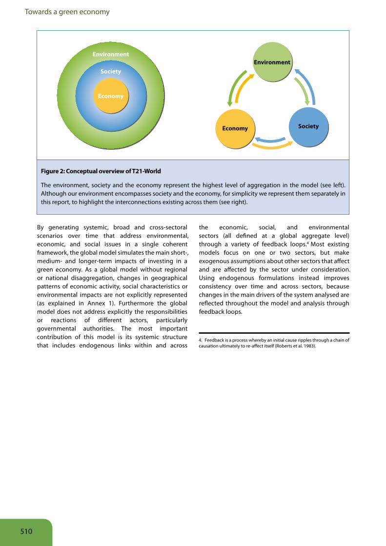
By generating systemic, broad and cross-sectoral scenarios over time that address environmental, economic, and social issues in a single coherent framework, the global model simulates the main short-, medium- and longer-term impacts of investing in a green economy. As a global model without regional or national disaggregation, changes in geographical patterns of economic activity, social characteristics or environmental impacts are not explicitly represented (as explained in Annex 1). Furthermore the global model does not address explicitly the responsibilities or reactions of different actors, particularly governmental authorities. The most important contribution of this model is its systemic structure that includes endogenous links within and across
the economic, social, and environmental sectors (all defined at a global aggregate level) through a variety of feedback loops.4 Most existing models focus on one or two sectors, but make exogenous assumptions about other sectors that affect and are affected by the sector under consideration. Using endogenous formulations instead improves consistency over time and across sectors, because changes in the main drivers of the system analysed are reflected throughout the model and analysis through feedback loops.
4. Feedback is a process whereby an initial cause ripples through a chain of causation ultimately to re-affect itself (Roberts et al. 1983).
Society
Environment
Society
Economy
Economy
Environment
Figure 2: Conceptual overview of T21-World
The environment, society and the economy represent the highest level of aggregation in the model (see left). Although our environment encompasses society and the economy, for simplicity we represent them separately in this report, to highlight the interconnections existing across them (see right).
510
Modelling
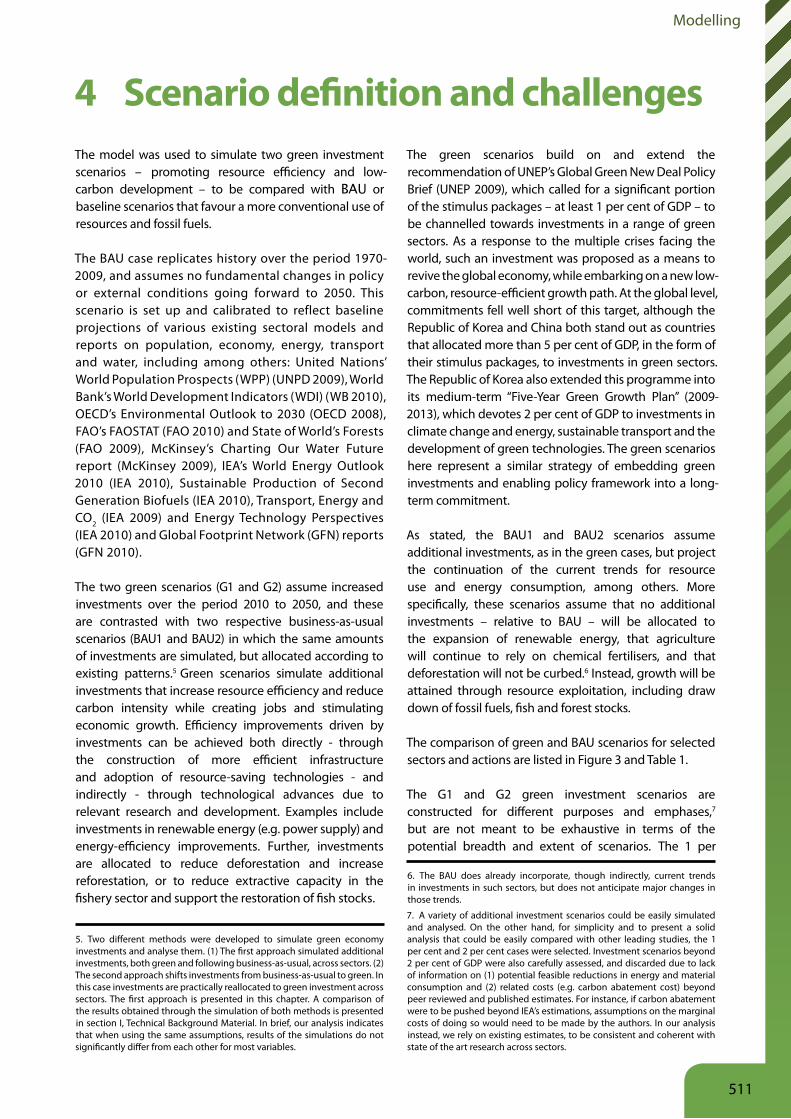
4 Scenario definition and challengesThe model was used to simulate two green investment scenarios – promoting resource efficiency and low-carbon development – to be compared with BAU or baseline scenarios that favour a more conventional use of resources and fossil fuels.
The BAU case replicates history over the period 1970-2009, and assumes no fundamental changes in policy or external conditions going forward to 2050. This scenario is set up and calibrated to reflect baseline projections of various existing sectoral models and reports on population, economy, energy, transport and water, including among others: United Nations’ World Population Prospects (WPP) (UNPD 2009), World Bank’s World Development Indicators (WDI) (WB 2010), OECD’s Environmental Outlook to 2030 (OECD 2008), FAO’s FAOSTAT (FAO 2010) and State of World’s Forests (FAO 2009), McKinsey’s Charting Our Water Future report (McKinsey 2009), IEA’s World Energy Outlook 2010 (IEA 2010), Sustainable Production of Second Generation Biofuels (IEA 2010), Transport, Energy and CO2 (IEA 2009) and Energy Technology Perspectives (IEA 2010) and Global Footprint Network (GFN) reports (GFN 2010).
The two green scenarios (G1 and G2) assume increased investments over the period 2010 to 2050, and these are contrasted with two respective business-as-usual scenarios (BAU1 and BAU2) in which the same amounts of investments are simulated, but allocated according to existing patterns.5 Green scenarios simulate additional investments that increase resource efficiency and reduce carbon intensity while creating jobs and stimulating economic growth. Efficiency improvements driven by investments can be achieved both directly - through the construction of more efficient infrastructure and adoption of resource-saving technologies - and indirectly - through technological advances due to relevant research and development. Examples include investments in renewable energy (e.g. power supply) and energy-efficiency improvements. Further, investments are allocated to reduce deforestation and increase reforestation, or to reduce extractive capacity in the fishery sector and support the restoration of fish stocks.
5. Two different methods were developed to simulate green economy investments and analyse them. (1) The first approach simulated additional investments, both green and following business-as-usual, across sectors. (2) The second approach shifts investments from business-as-usual to green. In this case investments are practically reallocated to green investment across sectors. The first approach is presented in this chapter. A comparison of the results obtained through the simulation of both methods is presented in section I, Technical Background Material. In brief, our analysis indicates that when using the same assumptions, results of the simulations do not significantly differ from each other for most variables.
The green scenarios build on and extend the recommendation of UNEP’s Global Green New Deal Policy Brief (UNEP 2009), which called for a significant portion of the stimulus packages – at least 1 per cent of GDP – to be channelled towards investments in a range of green sectors. As a response to the multiple crises facing the world, such an investment was proposed as a means to revive the global economy, while embarking on a new low-carbon, resource-efficient growth path. At the global level, commitments fell well short of this target, although the Republic of Korea and China both stand out as countries that allocated more than 5 per cent of GDP, in the form of their stimulus packages, to investments in green sectors. The Republic of Korea also extended this programme into its medium-term “Five-Year Green Growth Plan” (2009-2013), which devotes 2 per cent of GDP to investments in climate change and energy, sustainable transport and the development of green technologies. The green scenarios here represent a similar strategy of embedding green investments and enabling policy framework into a long-term commitment.
As stated, the BAU1 and BAU2 scenarios assume additional investments, as in the green cases, but project the continuation of the current trends for resource use and energy consumption, among others. More specifically, these scenarios assume that no additional investments – relative to BAU – will be allocated to the expansion of renewable energy, that agriculture will continue to rely on chemical fertilisers, and that deforestation will not be curbed.6 Instead, growth will be attained through resource exploitation, including draw down of fossil fuels, fish and forest stocks.
The comparison of green and BAU scenarios for selected sectors and actions are listed in Figure 3 and Table 1.
The G1 and G2 green investment scenarios are constructed for different purposes and emphases,7 but are not meant to be exhaustive in terms of the potential breadth and extent of scenarios. The 1 per
6. The BAU does already incorporate, though indirectly, current trends in investments in such sectors, but does not anticipate major changes in those trends.
7. A variety of additional investment scenarios could be easily simulated and analysed. On the other hand, for simplicity and to present a solid analysis that could be easily compared with other leading studies, the 1 per cent and 2 per cent cases were selected. Investment scenarios beyond 2 per cent of GDP were also carefully assessed, and discarded due to lack of information on (1) potential feasible reductions in energy and material consumption and (2) related costs (e.g. carbon abatement cost) beyond peer reviewed and published estimates. For instance, if carbon abatement were to be pushed beyond IEA’s estimations, assumptions on the marginal costs of doing so would need to be made by the authors. In our analysis instead, we rely on existing estimates, to be consistent and coherent with state of the art research across sectors.
511
Towards a green economy
cent case (G1) is an experimental exercise to clarify and illustrate the concept of green economy – as it assumes an about equal allocation of funds across the sectors analysed – and to compare the projected impacts of the implementation of a green economy strategy with, among others, climate scenarios such as IEA’s 450 case. On the other hand, the 2 per cent case (G2) can be considered more relevant and coherent. In this case, current key issues, such as climate change, water scarcity and food security, determine the allocation of the investment across sectors. Being central to addressing climate change, energy investments are prioritised in this scenario to reach the emissions targets of IEA’s 450 and BLUE Map scenarios. It is important to note that, for the most part and unless otherwise stated, the sectoral chapters in the GER refer to G2 as the green investment scenario.
More specifically, these scenarios include investments in agriculture, fisheries, forestry, water, waste and energy, also allocated across sectors, such as industries, transportation, buildings and tourism. Cities are also analysed. More details on the scenarios follow:
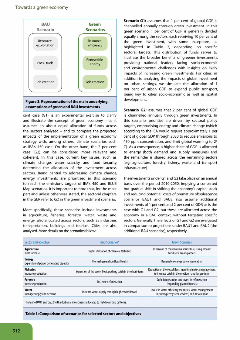
Scenario G1: assumes that 1 per cent of global GDP is channelled annually through green investment. In this green scenario, 1 per cent of GDP is generally divided equally among the sectors, each receiving 10 per cent of the green investment, with some exceptions, as highlighted in Table 2, depending on specific sectoral targets. This distribution of funds serves to illustrate the broader benefits of greener investments, providing national leaders facing socio-economic and environmental challenges with insights on likely impacts of increasing green investments. For cities, in addition to analysing the impacts of global investment on urban settings, we simulate the allocation of 1 per cent of urban GDP to expand public transport, being key to cities’ socio-economic as well as spatial development.
Scenario G2: assumes that 2 per cent of global GDP is channelled annually through green investments. In this scenario, priorities are driven by sectoral policy targets, emphasising energy and climate change (which according to the IEA would require approximately 1 per cent of global GDP through 2030 to reduce emissions to 450 ppm concentration, and limit global warming to 2o C). As a consequence, a higher share of GDP is allocated to energy (both demand and supply measures) and the remainder is shared across the remaining sectors (e.g. agriculture, forestry, fishery, waste and transport infrastructure).
The investments under G1 and G2 take place on an annual basis over the period 2010-2050, implying a concerted but gradual shift in shifting the economy’s capital stock and reducing potential: costs of premature obsolescence. Scenarios BAU1 and BAU2 also assume additional investments of 1 per cent and 2 per cent of GDP, as is the case with G1 and G2, but these are allocated across the economy in a BAU context, without targeting specific sectors. Generally, the effects of G1 and G2 are evaluated in comparison to projections under BAU1 and BAU2 (the additional BAU scenarios), respectively.
Table 1: Comparison of scenarios for selected sectors and objectives
Sector and objective BAU Scenariosa Green Scenarios
AgricultureYield increase Higher utilisation of chemical fertilisers Expansion of conservation agriculture, using organic
fertilisers, among others
EnergyExpansion of power generating capacity Thermal generation (fossil fuels) Renewable energy power generation
FisheriesIncrease production Expansion of the vessel fleet, pushing catch in the short-term Reduction of the vessel fleet, investing in stock management
to increase catch in the medium- and longer-term
ForestryIncrease production Increase deforestation Curb deforestation and invest in reforestation
(expanding planted forests)
WaterManage supply and demand Increase water supply through higher withdrawal Invest in water efficiency measures, water management
(including ecosystem services) and desalination
a Refers to BAU1 and BAU2 with additional investments allocated to match existing patterns.
BAUScenario
Green Scenarios
Resource exploitation
Resource e�ciency
Fossil fuelsRenewable
energy
Job creation Job creation
Figure 3: Representation of the main underlying assumptions of green and BAU investments
512
Modelling
4.1 Defining investments and methodology It is worth noting that a variety of policies are simulated together with the allocation of investments to green sectors. In fact, our scenarios account for both public and private investments, and assume that the total amount allocated is effectively spent across sectors. For this reason, when we refer to investment, we consider both public and private expenditure. The former can be represented by fiscal policies to stimulate the purchase of more efficient capital (e.g. tax rebates for purchasing a fuel efficient car, or a refrigerator) and the latter is the actual private expenditure to make the purchase. In addition, investment is generally referred
8. Investments allocated to cities are not presented in this table. Modelling work on cities has proven difficult to carry out do to the lack of data on a variety of key variables, including water and energy consumption. Emphasis was therefore put only on transport, as indicated in the Cities Chapter, given its relevance to urban development.
to here in its economic sense as increases to fixed capital, including infrastructure.9 It will be important to develop criteria and indicators that can be used to monitor relevant investments under eventual green investment scenarios.
In the modelling exercise, the source of funding for green investments is not explicitly defined. This is due to the fact that different governments, facing different constraints and being characterised by very heterogeneous contexts, may prefer to rely on different policies and schemes to support the transition to a green economy.
9. For some sectors, including natural-resource based sectors, such as agriculture, forestry and fisheries, investments included under the green investment scenarios do have a broader character, including expenditure on programmes (both capital and operating costs) to restore or maintain natural capital. These can also be considered as investments in natural capital in an economic sense, even though such investments have an indirect nature.
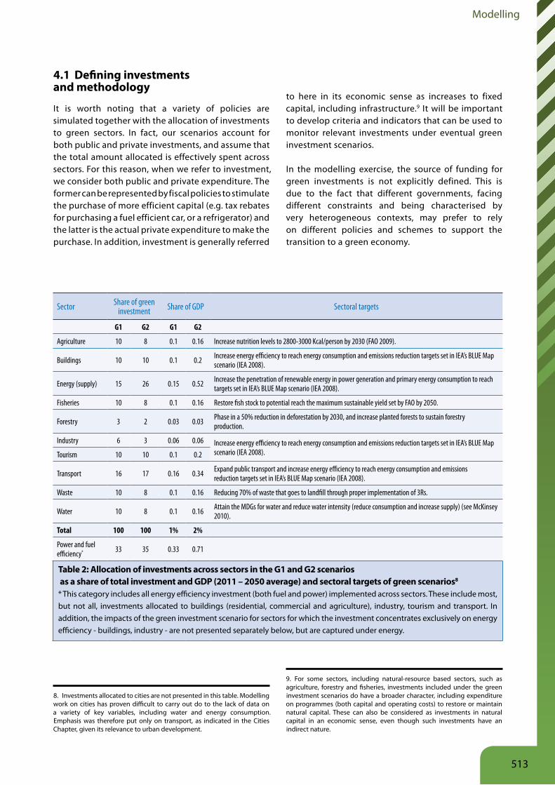
Sector Share of green investment Share of GDP Sectoral targets
G1 G2 G1 G2
Agriculture 10 8 0.1 0.16 Increase nutrition levels to 2800-3000 Kcal/person by 2030 (FAO 2009).
Buildings 10 10 0.1 0.2 Increase energy efficiency to reach energy consumption and emissions reduction targets set in IEA’s BLUE Map scenario (IEA 2008).
Energy (supply) 15 26 0.15 0.52 Increase the penetration of renewable energy in power generation and primary energy consumption to reach targets set in IEA’s BLUE Map scenario (IEA 2008).
Fisheries 10 8 0.1 0.16 Restore fish stock to potential reach the maximum sustainable yield set by FAO by 2050.
Forestry 3 2 0.03 0.03 Phase in a 50% reduction in deforestation by 2030, and increase planted forests to sustain forestry production.
Industry 6 3 0.06 0.06 Increase energy efficiency to reach energy consumption and emissions reduction targets set in IEA’s BLUE Map scenario (IEA 2008).Tourism 10 10 0.1 0.2
Transport 16 17 0.16 0.34 Expand public transport and increase energy efficiency to reach energy consumption and emissions reduction targets set in IEA’s BLUE Map scenario (IEA 2008).
Waste 10 8 0.1 0.16 Reducing 70% of waste that goes to landfill through proper implementation of 3Rs.
Water 10 8 0.1 0.16 Attain the MDGs for water and reduce water intensity (reduce consumption and increase supply) (see McKinsey 2010).
Total 100 100 1% 2%
Power and fuel efficiency* 33 35 0.33 0.71
Table 2: Allocation of investments across sectors in the G1 and G2 scenarios as a share of total investment and GDP (2011 – 2050 average) and sectoral targets of green scenarios8
* This category includes all energy efficiency investment (both fuel and power) implemented across sectors. These include most, but not all, investments allocated to buildings (residential, commercial and agriculture), industry, tourism and transport. In addition, the impacts of the green investment scenario for sectors for which the investment concentrates exclusively on energy efficiency - buildings, industry - are not presented separately below, but are captured under energy.
513
Towards a green economy
Further, as opposed to several studies that only provide information on “net costs” (or required additional investments),10 disaggregated capital costs and savings (or avoided costs) are used in T21-World. This approach is useful because as capital costs are an immediate expenditure, as opposed to operational savings – that are accumulated over the lifetime of capital – it allows the model to calculate the actual capital formation that corresponds to the additional investment simulated in the green and BAU1, 2 scenarios.
As indicated above, the calculation of required capital investment and operational costs includes a detailed assessment of costs associated with various technologies (capital) and their required inputs (e.g. energy). For instance, we account for the capital and O&M cost of a wind turbine, which, on a per MW basis, is often similar to the cost of a coal-fired plant. On the other hand, wind does not require fuel inputs and does not generate emissions, but it is an intermittent source of energy with a relatively low capacity factor when compared to coal. All these factors are considered in our analysis to break down as much as possible the costs and savings related to green investments.
Determining both the gross and net cost of moving toward a green economy has various purposes. These include the need to estimate (and disaggregate) present costs and future benefits for the key actors involved, both in economic terms and expressed as preservation of natural resource stocks. Also, it supports the further evaluation of the impact of policy options in light of the associated opportunities and risks. For instance, if a government has set an environmental goal (e.g. reducing emissions below 1990 levels) and decides to rely considerably on incentives (e.g. tax breaks or discounts) to support the shift from old to new capital and/or to more sustainable consumption, the buy-in of households and the private sector will be a key factor defining the success or failure of the policy. In this case, the government risks missing the targets and goals for emissions reduction; at the same time, if the private sector does not participate as expected, the economic expenses of the government (and the private sector) would be also be less. This policy option normally targets negotiated goals to mitigate the economic burden on households and the private sector. As an alternative case, when governments set mandates, the buy-in of households and private sector is assured by law, and the economic cost is either shared (if incentives are put into place) or fully sustained by
10. When considering the cost of purchasing, for instance, a more efficient refrigerator, the net cost is calculated as capital expenditure minus savings occurred in the operation of the refrigeration (i.e. savings originating from the reduced energy consumption). This is the case of McKinsey Cost Curves (for water see McKinsey 2009).
households and the private sector. In this case emphasis is put on reaching the policy target (through mandates) and costs can be more easily estimated knowing that both economic actors (public or private, in different ways) will have to sustain the costs associated with the full implementation of the mandate.
This study serves primarily to quantify the impacts of investments, identify opportunities and avoid dead ends. Given that similar policies will be more or less successful in different countries, the global study is focused on the value of allocating funds to greener investments, providing a broad range of information to national policy makers, as presented in the following sections. Additional information on funding options and enabling conditions (i.e. required policy frameworks) are available in the respective chapters.
514
Modelling
5 Results of the simulations and analysis
5.1 Baseline projection (BAU)
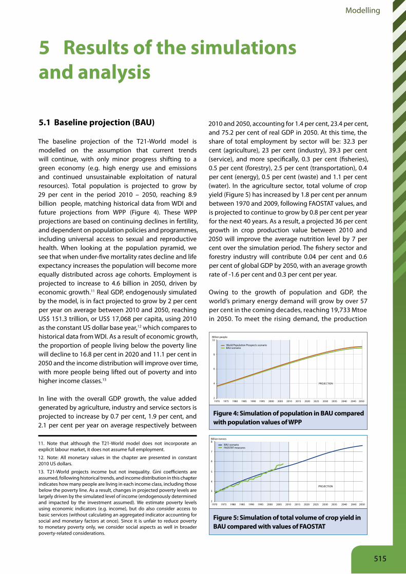
The baseline projection of the T21-World model is modelled on the assumption that current trends will continue, with only minor progress shifting to a green economy (e.g. high energy use and emissions and continued unsustainable exploitation of natural resources). Total population is projected to grow by 29 per cent in the period 2010 – 2050, reaching 8.9 billion people, matching historical data from WDI and future projections from WPP (Figure 4). These WPP projections are based on continuing declines in fertility, and dependent on population policies and programmes, including universal access to sexual and reproductive health. When looking at the population pyramid, we see that when under-five mortality rates decline and life expectancy increases the population will become more equally distributed across age cohorts. Employment is projected to increase to 4.6 billion in 2050, driven by economic growth.11 Real GDP, endogenously simulated by the model, is in fact projected to grow by 2 per cent per year on average between 2010 and 2050, reaching US$ 151.3 trillion, or US$ 17,068 per capita, using 2010 as the constant US dollar base year,12 which compares to historical data from WDI. As a result of economic growth, the proportion of people living below the poverty line will decline to 16.8 per cent in 2020 and 11.1 per cent in 2050 and the income distribution will improve over time, with more people being lifted out of poverty and into higher income classes.13
In line with the overall GDP growth, the value added generated by agriculture, industry and service sectors is projected to increase by 0.7 per cent, 1.9 per cent, and 2.1 per cent per year on average respectively between
11. Note that although the T21-World model does not incorporate an explicit labour market, it does not assume full employment.
12. Note: All monetary values in the chapter are presented in constant 2010 US dollars.
13. T21-World projects income but not inequality. Gini coefficients are assumed, following historical trends, and income distribution in this chapter indicates how many people are living in each income class, including those below the poverty line. As a result, changes in projected poverty levels are largely driven by the simulated level of income (endogenously determined and impacted by the investment assumed). We estimate poverty levels using economic indicators (e.g. income), but do also consider access to basic services (without calculating an aggregated indicator accounting for social and monetary factors at once). Since it is unfair to reduce poverty to monetary poverty only, we consider social aspects as well in broader poverty-related considerations.
2010 and 2050, accounting for 1.4 per cent, 23.4 per cent, and 75.2 per cent of real GDP in 2050. At this time, the share of total employment by sector will be: 32.3 per cent (agriculture), 23 per cent (industry), 39.3 per cent (service), and more specifically, 0.3 per cent (fisheries), 0.5 per cent (forestry), 2.5 per cent (transportation), 0.4 per cent (energy), 0.5 per cent (waste) and 1.1 per cent (water). In the agriculture sector, total volume of crop yield (Figure 5) has increased by 1.8 per cent per annum between 1970 and 2009, following FAOSTAT values, and is projected to continue to grow by 0.8 per cent per year for the next 40 years. As a result, a projected 36 per cent growth in crop production value between 2010 and 2050 will improve the average nutrition level by 7 per cent over the simulation period. The fishery sector and forestry industry will contribute 0.04 per cent and 0.6 per cent of global GDP by 2050, with an average growth rate of -1.6 per cent and 0.3 per cent per year.
Owing to the growth of population and GDP, the world’s primary energy demand will grow by over 57 per cent in the coming decades, reaching 19,733 Mtoe in 2050. To meet the rising demand, the production
Figure 4: Simulation of population in BAU compared with population values of WPP
Figure 5: Simulation of total volume of crop yield in BAU compared with values of FAOSTAT
21970 1975
World Population Prospects scenarioBAU scenario
1980 1985 1990 1995 2000 2005 2010 2015 2020
PROJECTION
2025 2030 2035 2040 2045 2050
4
6
8
10Billion people
21970 1975
BAU scenarioFAOSTAT measures
1980 1985 1990 1995 2000 2005 2010 2015 2020
PROJECTION
2025 2030 2035 2040 2045 2050
4
3
7
6
5
8Billion tonnes
515

Towards a green economy
of fossil fuels, nuclear and renewable energy will increase from 10,174 Mtoe, 755 Mtoe and 1,620 Mtoe respectively in 2011, to reach 16,073 Mtoe, 1,089 Mtoe, and 2,577 Mtoe respectively in 2050, with the share of fossil fuels remaining at 81 per cent throughout 2050.
For oil demand, among other fossil fuels, the simulated trends of growth in BAU and corresponding WEO values are illustrated in Figure 6. The projection of oil price follows IEA’s WEO, and increases faster after 2030, due to the peak of conventional oil projected to take place after 2035.
Driven by the same factors, total water consumption is projected to reach 8,141 km3 in 2050 – 70 per cent above its current value – with total water supply heavily relying on groundwater reservoirs and streams well beyond sustainable withdrawals. This production level would probably compromise aquifers, increasing salt-water infiltration in coastal areas and forcing massive migrations.
Concerning land use, total agricultural land will expand to 5.4 billion hectares by 2050, with pasture and arable land growing by 11 per cent and 6 per cent between 2010 and 2050. The harvested area in turn will reach 1.3 billion hectares by 2050, a 9 per cent increase relative to 2010 to meet the increasing food demand. In addition, settlement land will grow by 0.7 per cent per year on average, reaching 226 million hectares in 2050. Correspondingly, forestland will suffer from an average net loss of 6 million hectares per year and a deforestation rate of 15 million hectares per year, with only 3.7 billion hectares of forestland left by 2050. As a result, the total carbon storage in forests will decline by about 7 per cent between 2010 and 2050. The fishery sector will also face challenges such as declining stocks. The total amount of fish caught is projected to decline by as much as 46 per cent between 2010 and 2050, due to overcapacity and ineffective management of the industry and natural resources.
Finally, owing to the larger population and higher income, the world is expected to generate over 13.2 billion tonnes of waste in 2050, 19 per cent higher than the amount in 2009.
As a consequence of these trends, total world CO2 emissions are projected to increase throughout the simulation, with fossil fuel emissions reaching about 50 billion tonnes (Gt) per year in 2050, 71 per cent above 2009 and 138 per cent above 1990 emission levels (Figure 8). This increase corresponds also to a 26 per cent reduction in global carbon intensity (calculated as emissions per US$ of GDP) between 2009 and 2050. The transport sector, as a major emitter, will account of 13 Gt
Figure 6: Simulation of oil demand in BAU compared with values of WEO**For past and future projections, the model fits well with WEO values in terms of oil demand-R-square of 98.3 per cent and average point-to-point deviation 0.69 per cent.
Figure 7: Simulation of arable land and forestland in BAU compared with values of FAOSTAT
10 000
20 000
30 000
40 000
50 000
1970 1975
BAU scenarioWorld Energy Outlook
1980 1985 1990 1995 2000 2005 2010 2015 2020
PROJECTION
2025 2030 2035 2040 2045 2050
Million barrels
0
1
2
3
4
1970 1975 1980 1985 1990 1995 2000 2005 2010 2015 2020 2025 2030 2035 2040 2045 2050
Billion hectares
BAU scenarioFAOSTAT
Arable land
BAU scenarioFAOSTAT
Forestland
516
Modelling
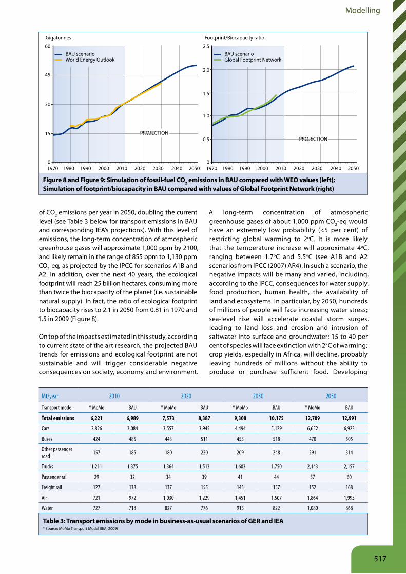
of CO2 emissions per year in 2050, doubling the current level (see Table 3 below for transport emissions in BAU and corresponding IEA’s projections). With this level of emissions, the long-term concentration of atmospheric greenhouse gases will approximate 1,000 ppm by 2100, and likely remain in the range of 855 ppm to 1,130 ppm CO2-eq, as projected by the IPCC for scenarios A1B and A2. In addition, over the next 40 years, the ecological footprint will reach 25 billion hectares, consuming more than twice the biocapacity of the planet (i.e. sustainable natural supply). In fact, the ratio of ecological footprint to biocapacity rises to 2.1 in 2050 from 0.81 in 1970 and 1.5 in 2009 (Figure 8).
On top of the impacts estimated in this study, according to current state of the art research, the projected BAU trends for emissions and ecological footprint are not sustainable and will trigger considerable negative consequences on society, economy and environment.
A long-term concentration of atmospheric greenhouse gases of about 1,000 ppm CO2-eq would have an extremely low probability (<5 per cent) of restricting global warming to 2oC. It is more likely that the temperature increase will approximate 4oC, ranging between 1.7oC and 5.5oC (see A1B and A2 scenarios from IPCC (2007) AR4). In such a scenario, the negative impacts will be many and varied, including, according to the IPCC, consequences for water supply, food production, human health, the availability of land and ecosystems. In particular, by 2050, hundreds of millions of people will face increasing water stress; sea-level rise will accelerate coastal storm surges, leading to land loss and erosion and intrusion of saltwater into surface and groundwater; 15 to 40 per cent of species will face extinction with 2°C of warming; crop yields, especially in Africa, will decline, probably leaving hundreds of millions without the ability to produce or purchase sufficient food. Developing
Figure 8 and Figure 9: Simulation of fossil-fuel CO2 emissions in BAU compared with WEO values (left); Simulation of footprint/biocapacity in BAU compared with values of Global Footprint Network (right)
Mt/year 2010 2020 2030 2050
Transport mode * MoMo BAU * MoMo BAU * MoMo BAU * MoMo BAU
Total emissions 6,221 6,989 7,573 8,387 9,308 10,175 12,709 12,991
Cars 2,826 3,084 3,557 3,945 4,494 5,129 6,652 6,923
Buses 424 485 443 511 453 518 470 505
Other passenger road 157 185 180 220 209 248 291 314
Trucks 1,211 1,375 1,364 1,513 1,603 1,750 2,143 2,157
Passenger rail 29 32 34 39 41 44 57 60
Freight rail 127 138 137 155 143 157 152 168
Air 721 972 1,030 1,229 1,451 1,507 1,864 1,995
Water 727 718 827 776 915 822 1,080 868
Table 3: Transport emissions by mode in business-as-usual scenarios of GER and IEA* Source: MoMo Transport Model (IEA, 2009)
0
15
30
45
60
1970
BAU scenarioWorld Energy Outlook
1980 1990 2000 2010 2020
PROJECTION
2030 2040 2050
Gigatonnes
0
0.5
1.5
1.0
2.0
2.5
1970
BAU scenarioGlobal Footprint Network
1980 1990 2000 2010 2020
PROJECTION
2030 2040 2050
Footprint/Biocapacity ratio
517
Towards a green economy
countries are the most vulnerable to climate change impacts. As many of the effects of climate change depend on the degree of adaptation, which itself will be determined by income levels and market structure, these countries have fewer resources to adapt socially, technologically and financially. It is estimated in Stern’s Review of the Economics of Climate Change (2006) that climate change will impose an overall cost equivalent to 0.5 to 1 per cent of world GDP per annum by the middle of the century if no emission mitigation measures are taken in the short- and medium-term. Further, the report indicates that if we start to take strong action now to achieve a stabilisation between 710ppm and 445ppm CO2-eq by 2050, the global average macro-economic costs for GHG mitigation are between negative 1 per cent and positive 5.5 per cent of global GDP, which is equivalent to slowing average annual global GDP growth by about 0.12 per cent per year.
In the GER BAU scenario, the feedback effects from natural resource depletion are sufficiently important that the annual rate of world GDP growth gradually
falls from about 2.7 per cent per year in the period 2010-2020 to 2.2 per cent in 2020-2030 and further to 1.6 per cent in 2030-2050.
5.2 Green economy projections
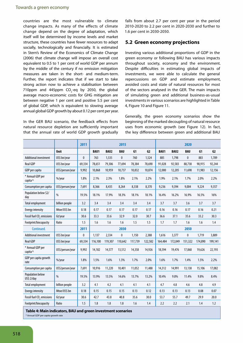
Investing various additional proportions of GDP in the green economy or following BAU has various impacts throughout society, economy and the environment. Despite difficulties in estimating global impacts of investments, we were able to calculate the general repercussions on GDP and estimate employment, avoided costs and state of natural resources for most of the sectors analysed in the GER. The main impacts of simulating green and additional business-as-usual investments in various scenarios are highlighted in Table 4, Figure 10 and Figure 11.
Generally, the green economy scenarios show the beginning of the marked decoupling of natural resource uses from economic growth (see Figure 12). In fact, the key difference between green and additional BAU
2011 2015 2020
Unit BAU1 BAU2 BAU G1 G2 BAU1 BAU2 BAU G1 G2
Additional investment US$ bn/year 0 763 1,535 0 760 1,524 885 1,798 0 883 1,789
Real GDP US$ bn/year 69,334 78,651 79,306 77,694 78,384 78,690 91,028 92,583 88,738 90,915 92,244
GDP per capita US$/person/year 9,992 10,868 10,959 10,737 10,832 10,874 12,000 12,205 11,698 11,983 12,156
* Annual GDP per capita^ %/year 1.8% 2.1% 2.3% 1.8% 2.1% 2.2% 1.9% 2.1% 1.7% 2.0% 2.2%
Consumption per capita US$/person/year 7,691 8,366 8,435 8,264 8,338 8,370 9,236 9,394 9,004 9,224 9,357
Population below $2/day % 19.5% 18.1% 17.9% 18.3% 18.1% 18.1% 16.4% 16.2% 16.9% 16.5% 16%
Total employment billion people 3.2 3.4 3.4 3.4 3.4 3.4 3.7 3.7 3.6 3.7 3.7
Energy intensity Mtoe/US$ bn 0.18 0.17 0.17 0.17 0.17 0.17 0.16 0.16 0.17 0.16 0.21
Fossil fuel CO2 emissions Gt/year 30.6 33.3 33.6 32.9 32.0 30.7 36.6 37.1 35.6 33.2 30.3
Footprint/biocapacity Ratio 1.5 1.6 1.6 1.6 1.5 1.5 1.7 1.7 1.6 1.6 1.4
Continued. 2011 2030 2050
Additional investment US$ bn/year 0 1,137 2,334 0 1,150 2,388 1,616 3,377 0 1,719 3,889
Real GDP US$ bn/year 69,334 116,100 119,307 110,642 117,739 122,582 164,484 172,049 151,322 174,890 199,141
* Annual GDP per capita^ US$/person/year 9,992 14,182 14,577 13,512 14,358 14,926 18,594 19,476 17,068 19,626 22,193
GDP per capita growth rate %/year 1.8% 1.5% 1.6% 1.3% 1.7% 2.0% 1.6% 1.7% 1.4% 1.5% 2.2%
Consumption per capita US$/person/year 7,691 10,916 11,220 10,401 11,052 11,488 14,312 14,991 13,138 15,106 17,082
Population below US$ 2/day % 19.5% 13.9% 13.5% 14.6% 13.7% 13.2% 10.4% 9.8% 11.4% 9.8% 8.4%
Total employment billion people 3.2 4.1 4.2 4.1 4.1 4.1 4.7 4.8 4.6 4.8 4.9
Energy intensity Mtoe/US$ bn 0.18 0.15 0.15 0.15 0.13 0.12 0.13 0.13 0.13 0.08 0.07
Fossil fuel CO2 emissions Gt/year 30.6 42.7 43.8 40.8 35.6 30.0 53.7 55.7 49.7 29.9 20.0
Footprint/biocapacity Ratio 1.5 1.8 1.8 1.8 1.6 1.4 2.2 2.2 2.1 1.4 1.2
Table 4: Main indicators, BAU and green investment scenarios* Annual GDP per capita growth rate
518
Modelling
investments is created by the projected future of stocks of natural resources (see Box 1, based on section VI in the Technical Background Material, which presents the changes in natural resource stocks in more detail, including estimates of changes in the value of natural capital assets and adjusted net domestic product –NDP). Business-as-usual scenarios push consumption, stimulating economic growth in the short- and medium-term, thus exacerbating known historical trends of depletion of natural resources. As a consequence, in the longer-term, the decline of natural resources (e.g. fish stocks, forestland and fossil fuels) will have a negative impact on GDP (i.e. through reduced production capacity, higher energy prices and growing emissions) and results in a lower level of employment. Additional consequences may include large-scale migration driven by resource shortages (e.g. water), faster global warming and considerable biodiversity losses.
The green scenarios, by promoting investment in key ecosystem services and low-carbon development, show slightly slower economic growth in the short- to medium-term, but faster and more sustainable growth in the longer-term. In this respect, the green scenarios show more resilience, by lowering emissions, reducing dependence on volatile fuels and using natural resources more efficiently and sustainably. In other words, the green economy investment scenarios take the earth off of the collision course it is currently on with biophysical constraints. A more detailed summary of key results across sectors is presented below.
Worth noting, while BAU investments show a higher return on investment (ROI) in the short- and medium-term, green investments indicate higher economic ROI in the longer-term, outperforming BAU investments by
over 25 per cent throughout 2050-yielding, on average by 2050 over US$ 3 for each US$ invested. Also, both investments yield positive economic returns after about nine to 11 years in the green cases and seven to 9 years in BAU scenarios. More specifically, it can be observed that BAU investments will drive faster economic growth – in terms of total and per capita GDP14 – than the green alternatives in the short-term, with only marginal difference in social improvements (poverty reduction, employment, nutrition). In the medium- to longer-term, however, the economic and social development in a green economy is expected to outperform the BAU cases. Moreover, the green scenarios always see lower negative impacts on the environment (e.g. energy intensity, emissions and footprint), which will contribute to the faster medium- to longer-term economic growth observed in green scenarios relative to BAU ones.
Results of the BAU and green scenarios indicate that global real GDP would reach between US$ 175 and US$ 199 trillion by 2050 respectively in the G1 and G2 scenarios, which exceeds the US$ 164 in the BAU1 and US$ 172 trillion in BAU2 cases, by 6 per cent and 16 per cent respectively. The average annual growth rate reaches, on average, 2.3-2.7 per cent between 2010 and 2050 in the green scenarios, although the relevant comparison is to the BAU1 and BAU2 scenarios. These latter scenarios see faster economic development in the short to medium term, with 2.3 per cent to 2.4 per cent annual growth rate between 2010 and 2050. However, GDP in the BAU1 and BAU2 scenarios in 2050 is lower than in G1 and G2, due to natural resource depletion and the higher energy costs (Figure 13). This can partly be seen in calculations of NDP adjusted for depreciation of both fossil fuel and fish stocks (see
14. Even by this limited, conventional measure, which does not represent progress nor wealth (See Box 1).
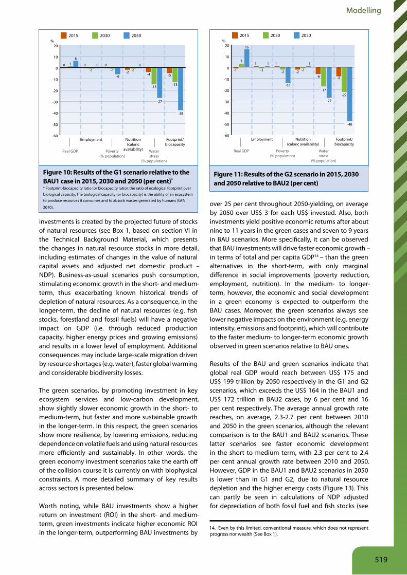
Figure 10: Results of the G1 scenario relative to the BAU1 case in 2015, 2030 and 2050 (per cent)*
* Footprint-biocapacity ratio (or biocapacity ratio): the ratio of ecological footprint over biological capacity. The biological capacity (or biocapacity) is the ability of an ecosystem to produce resources it consumes and to absorb wastes generated by humans (GFN
2010).
Figure 11: Results of the G2 scenario in 2015, 2030 and 2050 relative to BAU2 (per cent)
-60
-50
-40
-30
-20
-10
0
10
20
205020302015
Footprint/biocapacity
Waterstress
(% population)
Nutrition(caloric
availability)Poverty(% population)
Employment
Real GDP
%
-38
-27
0
-4
-15
-5
-13
-1-2-6
-100
-10
610
-60
-50
-40
-30
-20
-10
0
10
20
205020302015
Footprint/biocapacity
Waterstress
(% population)
Nutrition(caloric availability)
Poverty(% population)
Employment
Real GDP
%
-48
-27
1
-6
-17
-8
-22
-1-2
-14
-2
11
-1
1
16
3
-1
519
Towards a green economy
Box 1). Economic development in a green economy pushes total employment up to 4.8-4.9 billion in the G1 and G2 scenarios (3 per cent to 5 per cent above BAU) (see Table 4). Depending on the investment simulated, and its timing, the total net direct employment in green sectors may decline in the short-term (primarily due to a decline in the fishery and forestry sector employment15), to then converge or rise above BAU employment in the medium to long run. The employment gain is projected to range from 134 million to 238 million for the G1 and G2 scenarios, depending on the projected growth of sectors that depend on natural resources.16 In the additional BAU scenarios, employment is expected to range between 97 million and 176 million higher than BAU in 2050, which assumes, perhaps optimistically, that the trend of depletion of natural stocks does not inhibit production and employment growth. On the other hand, when accounting for the indirect employment effect across the economy as well (jobs created or lost in sectors depending on the ones analysed in more details in this study, e.g. fish distribution), we observe a growth in the range of 149 million to 251 million jobs for green
15. Employment in the fisheries sector, when adopting the second approach proposed in the Fishery Chapter (i.e. the reduction of fishing capacity will affect primarily large vessels and industrial production), will be reduced by only 1-1.2 m people in the short-term – as opposed to a loss of about 10 m direct jobs. In this case, employment in the fishery sector in the longer-term will be largely above the BAU cases.
16. As noted above, the T21-World model does not assume full employment. In addition to the further details on employment per sector are presented below, an additional analysis of employment impacts based on contributions by the ILO can be found at www.ilo.org/wcmsp5/groups/public/@ed_emp/@emp_ent/documents/publication/wcms_152065.pdf.
scenarios and 126 million to 223 million for BAU1 and BAU2 scenarios respectively by 2050. The results highlight the need to confront transition costs of greening, particularly with regard to retraining and repositioning labour for a lower carbon future.
More specifically on short-term impacts, world GDP will be slightly higher (less than 1 per cent in 2015 and 2020) in the additional BAU scenarios, relative to green cases. In 2020, total GDP in both scenarios will reach about US$ 91-92 trillion, or 2.5 per cent to 4 per cent above BAU. In accordance, total employment will be 8-21 million (or 0.2 per cent to 0.6 per cent) lower in a green economy than in BAU1 and BAU2 cases, respectively by 2020, while it will be 2 to 3 per cent higher in G1 and G2 when only net direct employment in green sectors is considered.
Pressure on natural resources increases as GDP grows, and tends to slow the rate of GDP growth in both BAU1 and BAU2. Lower soil quality, higher water stress and fossil fuel prices all impact GDP negatively, in turn impacting indicators such as the HDI. Natural resources have varied impacts on the ecological footprint, which pushes resource use to 2.2 times what the planet can sustainably generate by 2050 in the BAU2 case, from 1.5 times in 2010 and 1.7 times in 2020. In the G1 and G2 scenarios, while investments support the transition to a lower carbon and more resource efficient economy, they generate higher GDP, as well as greater energy and water demand than would otherwise have been the case. As a consequence, the impact of green investments on resource conservation will be
0
1.4 3.5
3.0
2.5
2.0
1.5
1.0
0.5
0
0.2
0.4
0.6
0.8
1.0
1.2
1.4
0.2
0.4
0.6
0.8
1.0
1.2
1990 2010 2030 2050 1990 2010 2030 2050
Relative �sh stock
Natural resources, relative to 1970 ratio
Annual GDPgrowth rate, %
Relative forest area Relative oil reserves
BAU G2 SCENARIO
Figure 12: Trends in GDP growth rate (right axis) and stocks of natural resources (left axis: oil discovered reserves, fish stock and forest stock, relative to 1970 levels), in the BAU and G2 scenarios
Stocks are better managed and saved for future generations in G2, while supporting GDP growth already in the medium- and longer-term.
520
Modelling
partially offset by the additional GDP and associated consumption. Synergies, as explained below, can be found in investments in energy efficiency and renewable energy among others, because they generate a net reduction in fossil fuel demand, which in turn pushes prices below the BAU projection and generates considerable savings (or avoided costs) over time, despite the impact of the rebound effect.
As a result of green investments, global energy demand and CO2 emissions will be mitigated considerably by 2050 relative to BAU (Figure 14). Even without explicitly modelling and analysing the positive impacts on emissions of transitioning to conservation agriculture,17 we project a concentration in the range of 500-600 ppm in the green scenarios.18 This indicates a moderate to unlikely probability that global warming will be limited to 2oC, as indicated in the IPCC AR4 report (IPCC 2007). More specifically, the projections result in a 36 per cent reduction in global energy intensity by 2030 in the G2 case, with the annual volume of energy-related CO2
emissions declining to 30-20 Gt in 2050 from 30.6 Gt in 2010, also a 40 per cent and 60 per cent below BAU in 2050 for the G1 and G2 scenarios respectively, which is more significant than the short-term mitigation (reducing BAU by 3 to 6 per cent in 2015 and 7 to 15 per cent in 2020). Non-energy related emissions from fertiliser use, deforestation and harvested land will be lower than BAU by 16 to 25 per cent, 33 per cent and 1 per cent in 2015, and 45 to 68 per cent, 55 per cent and 4 per cent, respectively in 2050. It is worth noting when considering the enactment of a cap and trade mechanism with carbon prices aligned with the recent US domestic proposal (reaching US$ 77 per tonne of CO2 by 2030 and US$ 221 by 2050, in constant US dollars at 2010 prices), that the reduction in emissions from the green economy investment would represent a savings in avoided permit costs of about US$ 1000-1,650 billion per year on average between 2012 and 2050.
Finally, under the green economy scenarios, the ecological footprint will also improve in the medium to long run after a slight increase in the short-term, with the biocapacity ratio reaching 1.5 (or 4 per cent to 6 per cent below BAU) in 2015 and then stabilising at 1.4-1.2 throughout 2050, well below 2.0 in the BAU and 2.21-2.4 in the BAU1 and BAU2 scenarios (See Figure 15), and years of life expectancy lost due to emissions will be reduced by 3.6 per cent and 7 per cent on average in the G1 and G2 cases.
17. Due to the lack of global estimations on soil carbon absorption under conservation agriculture practices.
18. The concentration of emissions could be lowered to 450 ppm when accounting for the potential carbon sequestration of organic and conservation agriculture. Conservative estimates for the annual global sequestration potential of OA amount to 2.4–4 Gt CO2-eq, while other estimates point at a potential of 6.5-11.7 or even more (see Müller and Davis (2009); Nelson et al. (2009).
Since the green investments simulated have economic impacts (e.g. GDP), as well as social (e.g. employment, poverty) and environmental impacts (e.g. energy consumption, emissions, land and water management), the context in which they are applied are particularly relevant to the analysis. Developing countries, such as sub-Saharan countries, facing extreme poverty and considerable challenges in reaching the Millennium Development Goals (MDGs) (World Bank 2007), are heavily dependent on agriculture and highly vulnerable to climatic changes. Improving socio-economic conditions, through higher access to water and energy, but also improved nutrition, and the efficient utilisation of natural resources are key goals of green economy strategies in these countries. Developing countries strive to improve productivity and increase their economic resilience in order to sustain strong economic growth. Here, energy and resource efficiency are key to longer-term development. Equatorial nations, often endowed with oil and other natural resources, are a good example: being a net exporter of resources these countries can profit from a reduction in domestic demand, and by preserving forest and other stocks of natural resources - possibly through payments for ecosystem services - can maintain Earth’s biodiversity stocks. Finally, developed countries can more actively contribute to technology development and become a solid example of how mature economies can become resource efficient and reduce their carbon path, while creating jobs.
AgricultureIn the case of the green investment scenarios, the additional investment in the agriculture sector (US$ 118-US$ 198 billion per year on average in 2011-2050 in G1 and G2, respectively) is allocated to more extensive use of organic fertiliser, agricultural research and development, pest control, and food processing. In these scenarios, the volume of agricultural (crop) production (excluding livestock forestry and fishery), is projected to increase by 7 to 11 per cent in 2030 and 11 to 17 per cent in 2050 compared with BAU.19 Relative to BAU1 and BAU2, value added in the green cases will be between 3 and 5 per cent in 2030 and in the range of 5 to 9 per cent in 2050. This development is mainly due to higher yield per hectare (15 to 22 per cent higher than BAU and 6 to 10 per cent than additional BAU scenarios by 2050, with BAU1 and BAU2 having a higher yield than the green scenarios in the short- to medium-term only), driven by improved soil quality (thanks to the extensive use of organic fertilisers), R&D efforts and effective pest control. As is presented in Figure 16, natural crop yield per hectare depends on a number of primary factors, with the actual effective
19. When assuming that a price premium could be applied to certified products, or those goods originating from sustainable agriculture practices, the total value of agricultural GDP in the G1 and G2 cases would be on average 28 per cent higher than BAU1 and BAU2 and 40 per cent higher than BAU. This calculation assumes, among others, that producers have access to markets that demand (or reward) sustainable practices.
521
Towards a green economy
Box 1: Changes in natural capital stocks Conventional economic indicators, such as GDP, provide a distorted lens on economic performance particularly since such measures fail to reflect the extent to which production and consumption activities may be drawing down natural capital. By either depleting natural resources, or degrading the ability of ecosystems to deliver economic benefits, in terms of provision, regulating or cultural services, economic activity may be based on the depreciation of natural capital. Various alternative approaches to adjusting the system of national accounts and aggregate economic indicators are being refined and discussed at the international level (e.g. Integrated Environmental and Economic Accounting – SEEA*).
The T21 model tracks the evolution of various natural resource stocks over time as highlighted in Figure 12 and in more detail in section VI of the Technical Background Material. The green economy scenarios are characterised by investment in and recovery of these stocks, providing a basis for sustained income gains over the medium- to longer-term.
It is insightful to undertake some additional calculations, using relatively simplistic assumptions, to generate some sense of the potential economic magnitude of the improved management of natural capital. The table below presents changes in the value of three resource stocks-fossil fuels, forests and fisheries-over the short- and medium-term in both absolute terms and relative to GDP. The change in physical values for fossil fuels and fish is valued using estimates of the economic value (unit rent), and for forests, using estimates from TEEB. Following the methodology employed by the World Bank (2006), these estimates of depreciation (or appreciation-where changes below are positive), these amounts can be seen as reflecting additional components of a measure of negative net savings in global wealth (as could be represented in asset accounts following system of national accounts).
According to these calculations, annual drawing down fossil fuel stocks is equivalent to 1.8 per cent of current GDP. Under BAU, this remains roughly the same in the short-term and then rises in the medium- to longer-term. The G1 and G2 scenarios reverse this trend with this depreciation, as a ratio to GDP, declining over the period 2010-2050, reaching 0.5 per cent of GDP by 2050 under G2, reflecting the marked reduction in fossil fuel dependence of the global economy in this scenario.
Lower and upper bound values of the value of the depreciation of natural capital in the form of forest land are presented due to the wider range of uncertainty concerning global reference values (see section VI, Technical Background Material, which makes use of results from TEEB research). Current depreciation of forestland is thus estimated at between US$ 2.8 billion and US$ 2.6 trillion - spanning three orders of magnitude - which is between 0.01 per cent and 5.4 per cent as a proportion of GDP. Note that the higher range estimates are comparable to, and indeed well above, those for fossil fuels. The green scenarios considerably reduce this loss within the short-term and turn it around into modest positive growth - or appreciation instead of depreciation - by 2050.
Similar improvements can be seen in fish stocks. The current estimate of depletion of this natural asset is valued at US$ 116 billion per year, which is -0.24 per cent when expressed as a ratio to GDP. The green scenarios succeed in reducing this lost and over the medium- to longer-term, stabilising it or turning into a net appreciation.
Although a range of results is only presented for forest resources, due to the wide range of existing measures, the estimates for fossil fuels and fish could also be developed into ranges. These would, however, probably not have the same degree of variability as those for forests.
It is important to bear in mind that even though the results are presented in a way that makes comparison between the estimated depreciation of the different assets comparable, this should be done and interpreted with care. In particular, the three assets are not substitutes for each other. Fossil fuels are a source of energy. Forests, including how they are valued here, provided a range of provisioning and regulating services, both locally but also much more widely, including even globally. Fisheries provide a major source of protein and employment to a substantial proportion of the world’s population but many of these people would not be able to substitute forests for fisheries as a source of food and livelihoods, or vice-versa.
In general, the results underline the substantial economic significance of how the world is currently managing its natural capital, as well as the potential gains that can be won from pursuing a green economy strategy. This allows the global economy to invest in natural capital that is critical for sustained well-being, while reducing the dependence on fossil fuels.
522
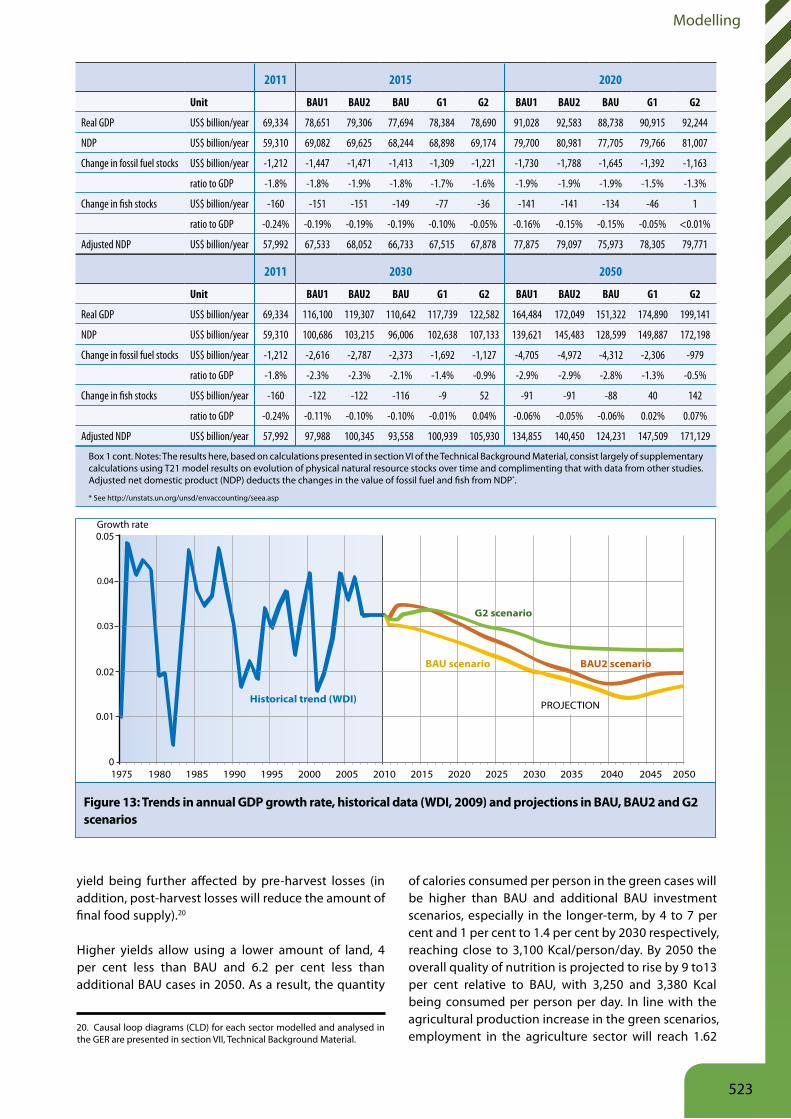
Modelling
yield being further affected by pre-harvest losses (in addition, post-harvest losses will reduce the amount of final food supply).20
Higher yields allow using a lower amount of land, 4 per cent less than BAU and 6.2 per cent less than additional BAU cases in 2050. As a result, the quantity
20. Causal loop diagrams (CLD) for each sector modelled and analysed in the GER are presented in section VII, Technical Background Material.
of calories consumed per person in the green cases will be higher than BAU and additional BAU investment scenarios, especially in the longer-term, by 4 to 7 per cent and 1 per cent to 1.4 per cent by 2030 respectively, reaching close to 3,100 Kcal/person/day. By 2050 the overall quality of nutrition is projected to rise by 9 to13 per cent relative to BAU, with 3,250 and 3,380 Kcal being consumed per person per day. In line with the agricultural production increase in the green scenarios, employment in the agriculture sector will reach 1.62
Figure 13: Trends in annual GDP growth rate, historical data (WDI, 2009) and projections in BAU, BAU2 and G2 scenarios
0
0.01
0.02
0.03
0.05
1975 1980 1985 1990 1995 2000 2005 2010 2015 2020
PROJECTION
2025 2030 2035 2040 2045 2050
Growth rate
BAU scenario BAU2 scenario
G2 scenario
Historical trend (WDI)
0.04
2011 2015 2020
Unit BAU1 BAU2 BAU G1 G2 BAU1 BAU2 BAU G1 G2
Real GDP US$ billion/year 69,334 78,651 79,306 77,694 78,384 78,690 91,028 92,583 88,738 90,915 92,244
NDP US$ billion/year 59,310 69,082 69,625 68,244 68,898 69,174 79,700 80,981 77,705 79,766 81,007
Change in fossil fuel stocks US$ billion/year -1,212 -1,447 -1,471 -1,413 -1,309 -1,221 -1,730 -1,788 -1,645 -1,392 -1,163
ratio to GDP -1.8% -1.8% -1.9% -1.8% -1.7% -1.6% -1.9% -1.9% -1.9% -1.5% -1.3%
Change in fish stocks US$ billion/year -160 -151 -151 -149 -77 -36 -141 -141 -134 -46 1
ratio to GDP -0.24% -0.19% -0.19% -0.19% -0.10% -0.05% -0.16% -0.15% -0.15% -0.05% <0.01%
Adjusted NDP US$ billion/year 57,992 67,533 68,052 66,733 67,515 67,878 77,875 79,097 75,973 78,305 79,771
2011 2030 2050
Unit BAU1 BAU2 BAU G1 G2 BAU1 BAU2 BAU G1 G2
Real GDP US$ billion/year 69,334 116,100 119,307 110,642 117,739 122,582 164,484 172,049 151,322 174,890 199,141
NDP US$ billion/year 59,310 100,686 103,215 96,006 102,638 107,133 139,621 145,483 128,599 149,887 172,198
Change in fossil fuel stocks US$ billion/year -1,212 -2,616 -2,787 -2,373 -1,692 -1,127 -4,705 -4,972 -4,312 -2,306 -979
ratio to GDP -1.8% -2.3% -2.3% -2.1% -1.4% -0.9% -2.9% -2.9% -2.8% -1.3% -0.5%
Change in fish stocks US$ billion/year -160 -122 -122 -116 -9 52 -91 -91 -88 40 142
ratio to GDP -0.24% -0.11% -0.10% -0.10% -0.01% 0.04% -0.06% -0.05% -0.06% 0.02% 0.07%
Adjusted NDP US$ billion/year 57,992 97,988 100,345 93,558 100,939 105,930 134,855 140,450 124,231 147,509 171,129
Box 1 cont. Notes: The results here, based on calculations presented in section VI of the Technical Background Material, consist largely of supplementary calculations using T21 model results on evolution of physical natural resource stocks over time and complimenting that with data from other studies. Adjusted net domestic product (NDP) deducts the changes in the value of fossil fuel and fish from NDP*.
* See http://unstats.un.org/unsd/envaccounting/seea.asp
523
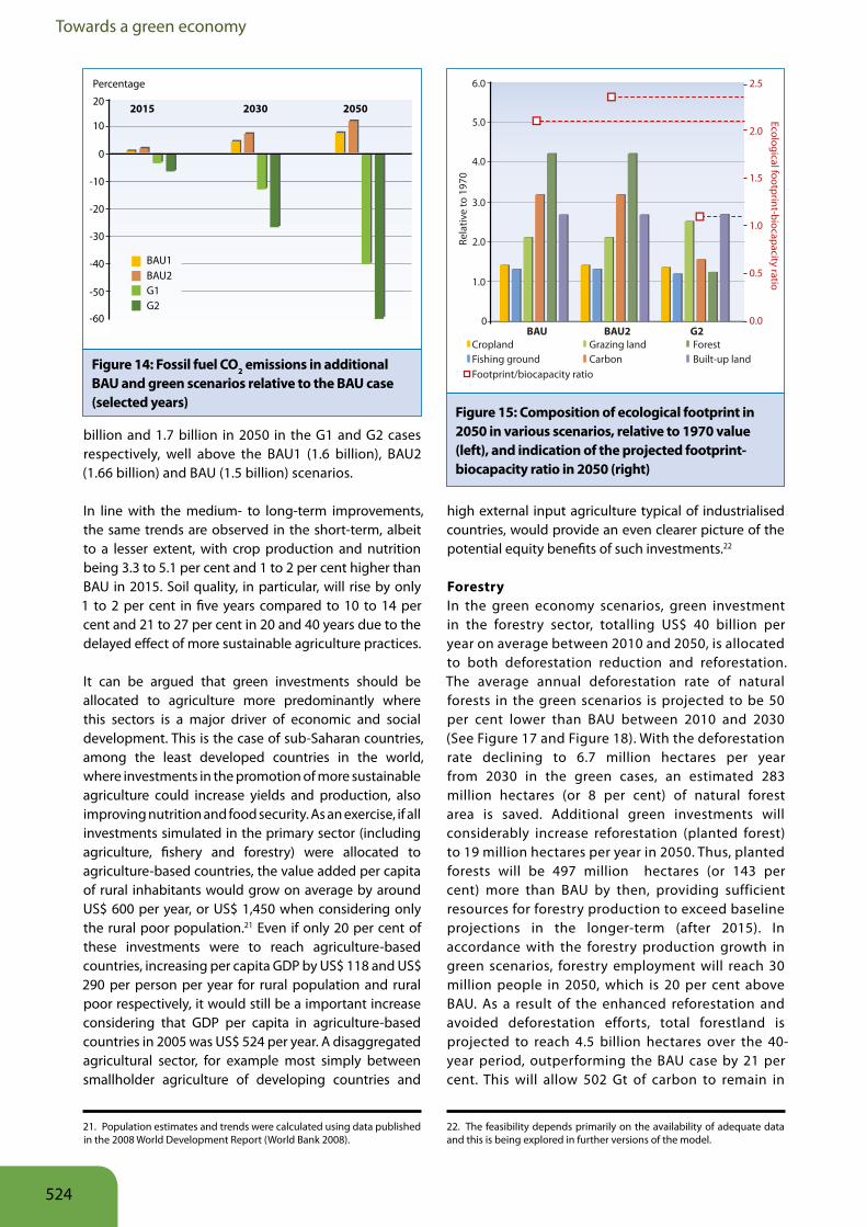
Towards a green economy
billion and 1.7 billion in 2050 in the G1 and G2 cases respectively, well above the BAU1 (1.6 billion), BAU2 (1.66 billion) and BAU (1.5 billion) scenarios.
In line with the medium- to long-term improvements, the same trends are observed in the short-term, albeit to a lesser extent, with crop production and nutrition being 3.3 to 5.1 per cent and 1 to 2 per cent higher than BAU in 2015. Soil quality, in particular, will rise by only 1 to 2 per cent in five years compared to 10 to 14 per cent and 21 to 27 per cent in 20 and 40 years due to the delayed effect of more sustainable agriculture practices.
It can be argued that green investments should be allocated to agriculture more predominantly where this sectors is a major driver of economic and social development. This is the case of sub-Saharan countries, among the least developed countries in the world, where investments in the promotion of more sustainable agriculture could increase yields and production, also improving nutrition and food security. As an exercise, if all investments simulated in the primary sector (including agriculture, fishery and forestry) were allocated to agriculture-based countries, the value added per capita of rural inhabitants would grow on average by around US$ 600 per year, or US$ 1,450 when considering only the rural poor population.21 Even if only 20 per cent of these investments were to reach agriculture-based countries, increasing per capita GDP by US$ 118 and US$ 290 per person per year for rural population and rural poor respectively, it would still be a important increase considering that GDP per capita in agriculture-based countries in 2005 was US$ 524 per year. A disaggregated agricultural sector, for example most simply between smallholder agriculture of developing countries and
21. Population estimates and trends were calculated using data published in the 2008 World Development Report (World Bank 2008).
high external input agriculture typical of industrialised countries, would provide an even clearer picture of the potential equity benefits of such investments.22
ForestryIn the green economy scenarios, green investment in the forestry sector, totalling US$ 40 billion per year on average between 2010 and 2050, is allocated to both deforestation reduction and reforestation. The average annual deforestation rate of natural forests in the green scenarios is projected to be 50 per cent lower than BAU between 2010 and 2030 (See Figure 17 and Figure 18). With the deforestation rate declining to 6.7 million hectares per year from 2030 in the green cases, an estimated 283 million hectares (or 8 per cent) of natural forest area is saved. Additional green investments will considerably increase reforestation (planted forest) to 19 million hectares per year in 2050. Thus, planted forests will be 497 million hectares (or 143 per cent) more than BAU by then, providing sufficient resources for forestry production to exceed baseline projections in the longer-term (after 2015). In accordance with the forestry production growth in green scenarios, forestry employment will reach 30 million people in 2050, which is 20 per cent above BAU. As a result of the enhanced reforestation and avoided deforestation efforts, total forestland is projected to reach 4.5 billion hectares over the 40-year period, outperforming the BAU case by 21 per cent. This will allow 502 Gt of carbon to remain in
22. The feasibility depends primarily on the availability of adequate data and this is being explored in further versions of the model.
Figure 14: Fossil fuel CO2 emissions in additional BAU and green scenarios relative to the BAU case (selected years)
Figure 15: Composition of ecological footprint in 2050 in various scenarios, relative to 1970 value (left), and indication of the projected footprint-biocapacity ratio in 2050 (right)
0
-10
-20
-30
-40
-50
-60
20
10
Percentage
BAU1
2015 2030 2050
BAU2G1G2
0
1.0
Cropland
Rela
tive
to 1
970
Ecological footprint-biocapacity ratio
BAU BAU2 G2
Fishing groundFootprint/biocapacity ratio
Grazing landCarbon
ForestBuilt-up land
3.0
4.0
6.0 2.5
2.0
1.5
1.0
0.5
0.0
2.0
5.0
524
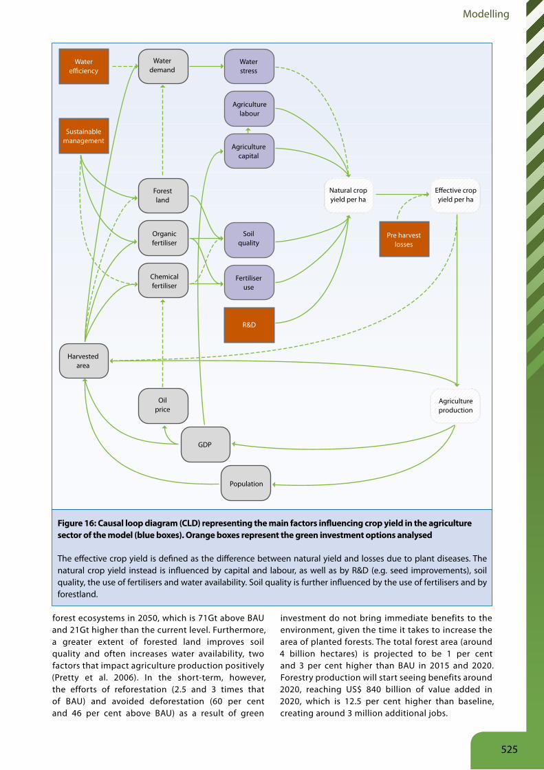
Modelling
forest ecosystems in 2050, which is 71Gt above BAU and 21Gt higher than the current level. Furthermore, a greater extent of forested land improves soil quality and often increases water availability, two factors that impact agriculture production positively (Pretty et al. 2006). In the short-term, however, the efforts of reforestation (2.5 and 3 times that of BAU) and avoided deforestation (60 per cent and 46 per cent above BAU) as a result of green
investment do not bring immediate benefits to the environment, given the time it takes to increase the area of planted forests. The total forest area (around 4 billion hectares) is projected to be 1 per cent and 3 per cent higher than BAU in 2015 and 2020. Forestry production will start seeing benefits around 2020, reaching US$ 840 billion of value added in 2020, which is 12.5 per cent higher than baseline, creating around 3 million additional jobs.
Water e�ciency
Water demand
Water stress
Agriculture labour
Agriculture capital
Natural crop yield per ha
E�ective crop yield per ha
Agriculture production
Soil quality
Organic fertiliser
Chemical fertiliser
Oil price
Harvested area
GDP
Population
Forest land
Fertiliseruse
R&D
Pre harvest losses
Sustainable management
Figure 16: Causal loop diagram (CLD) representing the main factors influencing crop yield in the agriculture sector of the model (blue boxes). Orange boxes represent the green investment options analysed
The effective crop yield is defined as the difference between natural yield and losses due to plant diseases. The natural crop yield instead is influenced by capital and labour, as well as by R&D (e.g. seed improvements), soil quality, the use of fertilisers and water availability. Soil quality is further influenced by the use of fertilisers and by forestland.
525
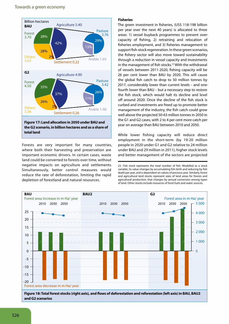
Towards a green economy
Forests are very important for many countries, where both their harvesting and preservation are important economic drivers. In certain cases, waste land could be converted to forests over time, without negative impacts on agriculture and settlements. Simultaneously, better control measures would reduce the rate of deforestation, limiting the rapid depletion of forestland and natural resources.
FisheriesThe green investment in fisheries, (US$ 118-198 billion per year over the next 40 years) is allocated to three areas: 1) vessel buyback programmes to prevent over-capacity of fishing, 2) retraining and relocation of fisheries employment, and 3) fisheries management to support fish-stock regeneration. In these green scenarios, the fishery sector will also move toward sustainability through a reduction in vessel capacity and investments in the management of fish stocks.23 With the withdrawal of vessels between 2011-2020, fishing capacity will be 26 per cent lower than BAU by 2020. This will cause the global fish catch to drop to 50 million tonnes by 2017, considerably lower than current levels – and one-fourth lower than BAU – but a necessary step to restore the fish stock, which would halt its decline and level off around 2020. Once the decline of the fish stock is curbed and investments are freed up to promote better management of the industry, the fish catch could grow well above the projected 50-63 million tonnes in 2050 in the G1 and G2 cases, with 2 to 4 per cent more catch per year on average than BAU between 2010 and 2050.
While lower fishing capacity will reduce direct employment in the short-term (by 19-20 million people in 2020 under G1 and G2 relative to 24 million under BAU and 29 million in 2011), higher stock levels and better management of the sectors are projected
23. Fish stock represents the total number of fish. Modelled as a stock variable, its value changes by accumulating fish birth and reducing by fish death per year, and is dependent on values of previous year. Similarly, forest and agricultural land stocks represent sizes of land areas for forests and agricultural production, that changes by annual conversion among types of land. Other stocks include resources of fossil fuels and water sources.
Figure 17: Land allocation in 2050 under BAU and the G2 scenario, in billion hectares and as a share of total land
Figure 18: Total forest stocks (right axis), and flows of deforestation and reforestation (left axis) in BAU, BAU2 and G2 scenarios
BAU
Forest3.70 28%
42%29%
13%
26%
11%37%
28%
35%
26%2%
2%
Agriculture 5.40
Others3.63 Settlement 0.22
Pasture3.76
Arable 1.65
Forest4.50
Agriculture 4.90
Others3.36 Settlement 0.26
Pasture3.42
Arable 1.46
Billion hectares
G2
0
5
10
-5
15
-10
20
-15
25
-20
0
1 000
2 000
3 000
4 000
5 0002010 2030 2050 2010 2030 2050 2010 2030 2050
BAU BAU2 G2
Forest area decrease in m Ha/ year
Forest area increase in m Ha/ year Forest area in m Ha/ year
area decrease in m Ha/ year
526
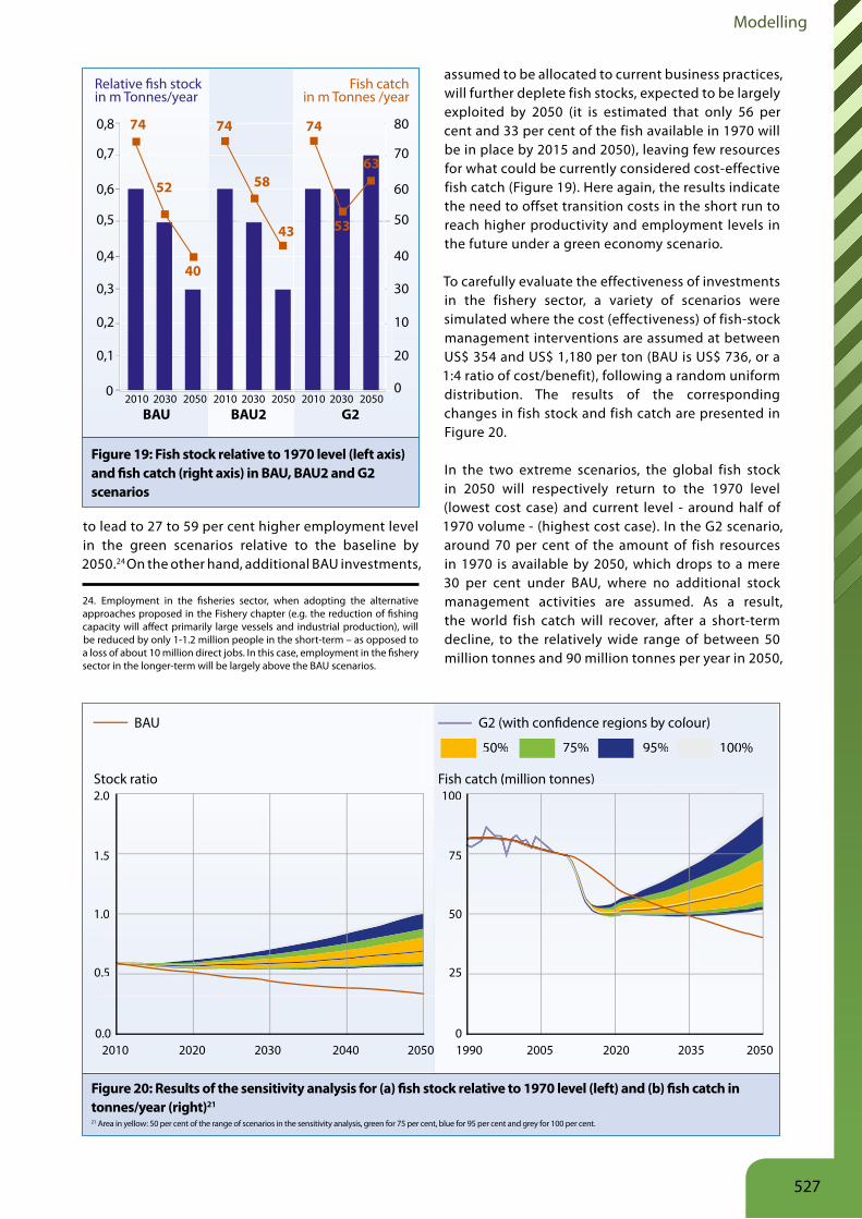
Modelling
to lead to 27 to 59 per cent higher employment level in the green scenarios relative to the baseline by 2050.24 On the other hand, additional BAU investments,
24. Employment in the fisheries sector, when adopting the alternative approaches proposed in the Fishery chapter (e.g. the reduction of fishing capacity will affect primarily large vessels and industrial production), will be reduced by only 1-1.2 million people in the short-term – as opposed to a loss of about 10 million direct jobs. In this case, employment in the fishery sector in the longer-term will be largely above the BAU scenarios.
assumed to be allocated to current business practices, will further deplete fish stocks, expected to be largely exploited by 2050 (it is estimated that only 56 per cent and 33 per cent of the fish available in 1970 will be in place by 2015 and 2050), leaving few resources for what could be currently considered cost-effective fish catch (Figure 19). Here again, the results indicate the need to offset transition costs in the short run to reach higher productivity and employment levels in the future under a green economy scenario.
To carefully evaluate the effectiveness of investments in the fishery sector, a variety of scenarios were simulated where the cost (effectiveness) of fish-stock management interventions are assumed at between US$ 354 and US$ 1,180 per ton (BAU is US$ 736, or a 1:4 ratio of cost/benefit), following a random uniform distribution. The results of the corresponding changes in fish stock and fish catch are presented in Figure 20.
In the two extreme scenarios, the global fish stock in 2050 will respectively return to the 1970 level (lowest cost case) and current level - around half of 1970 volume - (highest cost case). In the G2 scenario, around 70 per cent of the amount of fish resources in 1970 is available by 2050, which drops to a mere 30 per cent under BAU, where no additional stock management activities are assumed. As a result, the world fish catch will recover, after a short-term decline, to the relatively wide range of between 50 million tonnes and 90 million tonnes per year in 2050,
Figure 19: Fish stock relative to 1970 level (left axis) and fish catch (right axis) in BAU, BAU2 and G2 scenarios
Figure 20: Results of the sensitivity analysis for (a) fish stock relative to 1970 level (left) and (b) fish catch in tonnes/year (right)21
21 Area in yellow: 50 per cent of the range of scenarios in the sensitivity analysis, green for 75 per cent, blue for 95 per cent and grey for 100 per cent.
0,8
0,7
0,6
0,5
0,4
0,3
0,2
0,1
0
10
30
50
70
80
0
20
40
60
Relative �sh stockin m Tonnes/year
Fish catchin m Tonnes /year
74
40
52
74
43
58
74
63
53
2010 2030 20502010 2030 20502010 2030 2050BAU BAU2 G2
Stock ratio Fish catch (million tonnes)
BAU
50% 75% 95% 100%
G2 (with con�dence regions by colour)
2010 2020 2030 2040 2050 1990 2005 2020 2035 2050
0.5
1.0
1.5
2.0
0.0
25
50
75
100
0
Fish catch (
50%
G2 (w
(million tonne
% 75%
with con�den
(
%
(w
es)
% 95%
nce regions by
e
%
n
% 100
y colour)
%
y
50
75
00
0.5
.0
2
5
527
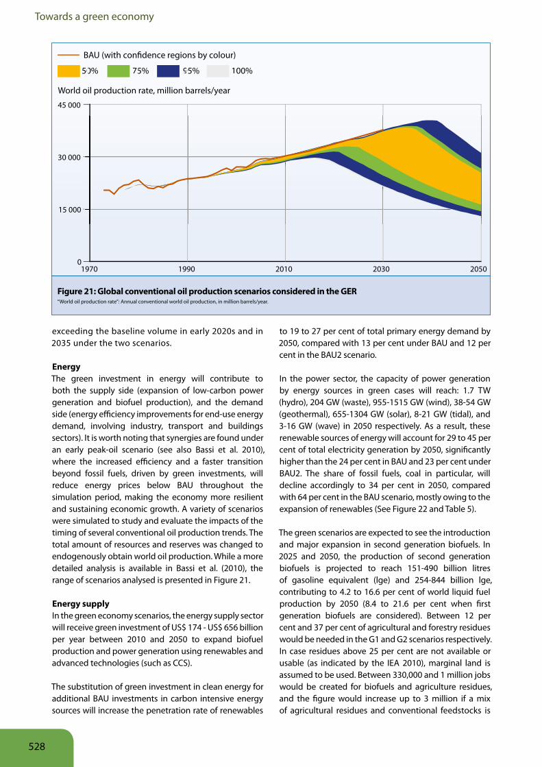
Towards a green economy
exceeding the baseline volume in early 2020s and in 2035 under the two scenarios.
EnergyThe green investment in energy will contribute to both the supply side (expansion of low-carbon power generation and biofuel production), and the demand side (energy efficiency improvements for end-use energy demand, involving industry, transport and buildings sectors). It is worth noting that synergies are found under an early peak-oil scenario (see also Bassi et al. 2010), where the increased efficiency and a faster transition beyond fossil fuels, driven by green investments, will reduce energy prices below BAU throughout the simulation period, making the economy more resilient and sustaining economic growth. A variety of scenarios were simulated to study and evaluate the impacts of the timing of several conventional oil production trends. The total amount of resources and reserves was changed to endogenously obtain world oil production. While a more detailed analysis is available in Bassi et al. (2010), the range of scenarios analysed is presented in Figure 21.
Energy supplyIn the green economy scenarios, the energy supply sector will receive green investment of US$ 174 - US$ 656 billion per year between 2010 and 2050 to expand biofuel production and power generation using renewables and advanced technologies (such as CCS).
The substitution of green investment in clean energy for additional BAU investments in carbon intensive energy sources will increase the penetration rate of renewables
to 19 to 27 per cent of total primary energy demand by 2050, compared with 13 per cent under BAU and 12 per cent in the BAU2 scenario.
In the power sector, the capacity of power generation by energy sources in green cases will reach: 1.7 TW (hydro), 204 GW (waste), 955-1515 GW (wind), 38-54 GW (geothermal), 655-1304 GW (solar), 8-21 GW (tidal), and 3-16 GW (wave) in 2050 respectively. As a result, these renewable sources of energy will account for 29 to 45 per cent of total electricity generation by 2050, significantly higher than the 24 per cent in BAU and 23 per cent under BAU2. The share of fossil fuels, coal in particular, will decline accordingly to 34 per cent in 2050, compared with 64 per cent in the BAU scenario, mostly owing to the expansion of renewables (See Figure 22 and Table 5).
The green scenarios are expected to see the introduction and major expansion in second generation biofuels. In 2025 and 2050, the production of second generation biofuels is projected to reach 151-490 billion litres of gasoline equivalent (lge) and 254-844 billion lge, contributing to 4.2 to 16.6 per cent of world liquid fuel production by 2050 (8.4 to 21.6 per cent when first generation biofuels are considered). Between 12 per cent and 37 per cent of agricultural and forestry residues would be needed in the G1 and G2 scenarios respectively. In case residues above 25 per cent are not available or usable (as indicated by the IEA 2010), marginal land is assumed to be used. Between 330,000 and 1 million jobs would be created for biofuels and agriculture residues, and the figure would increase up to 3 million if a mix of agricultural residues and conventional feedstocks is
Figure 21: Global conventional oil production scenarios considered in the GER“World oil production rate”: Annual conventional world oil production, in million barrels/year.
World oil production rate, million barrels/year
BAU (with con�dence regions by colour)
50% 75% 95% 100%
1970 1990 2010 2030 2050
15 000
30 000
45 000
0
50 75 9 10
528
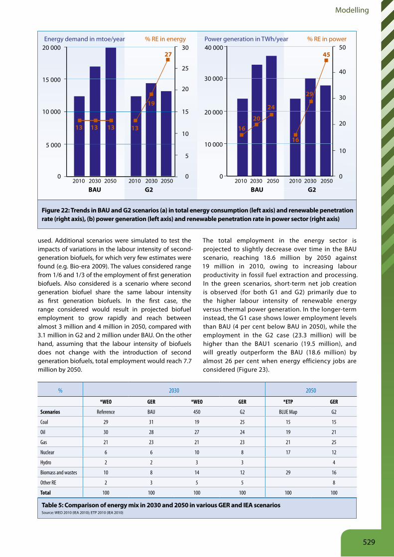
Modelling
used. Additional scenarios were simulated to test the impacts of variations in the labour intensity of second-generation biofuels, for which very few estimates were found (e.g. Bio-era 2009). The values considered range from 1/6 and 1/3 of the employment of first generation biofuels. Also considered is a scenario where second generation biofuel share the same labour intensity as first generation biofuels. In the first case, the range considered would result in projected biofuel employment to grow rapidly and reach between almost 3 million and 4 million in 2050, compared with 3.1 million in G2 and 2 million under BAU. On the other hand, assuming that the labour intensity of biofuels does not change with the introduction of second generation biofuels, total employment would reach 7.7 million by 2050.
The total employment in the energy sector is projected to slightly decrease over time in the BAU scenario, reaching 18.6 million by 2050 against 19 million in 2010, owing to increasing labour productivity in fossil fuel extraction and processing. In the green scenarios, short-term net job creation is observed (for both G1 and G2) primarily due to the higher labour intensity of renewable energy versus thermal power generation. In the longer-term instead, the G1 case shows lower employment levels than BAU (4 per cent below BAU in 2050), while the employment in the G2 case (23.3 million) will be higher than the BAU1 scenario (19.5 million), and will greatly outperform the BAU (18.6 million) by almost 26 per cent when energy efficiency jobs are considered (Figure 23).
Figure 22: Trends in BAU and G2 scenarios (a) in total energy consumption (left axis) and renewable penetration rate (right axis), (b) power generation (left axis) and renewable penetration rate in power sector (right axis)
% 2030 2050
*WEO GER *WEO GER *ETP GER
Scenarios Reference BAU 450 G2 BLUE Map G2
Coal 29 31 19 25 15 15
Oil 30 28 27 24 19 21
Gas 21 23 21 23 21 25
Nuclear 6 6 10 8 17 12
Hydro 2 2 3 3 4
Biomass and wastes 10 8 14 12 29 16
Other RE 2 3 5 5 8
Total 100 100 100 100 100 100
Table 5: Comparison of energy mix in 2030 and 2050 in various GER and IEA scenariosSource: WEO 2010 (IEA 2010); ETP 2010 (IEA 2010)
0
5
10
15
20
25
3020 000
15 000
10 000
5 000
0
40 000
30 000
20 000
10 000
02010 2030 2050 2010 2030 2050 2010 2030 2050 2010 2030 2050
BAU
Energy demand in mtoe/year Power generation in TWh/year
G2 BAU G2
0
10
20
30
40
50% RE in energy % RE in power
13 1313 13
27
19
16
24
20
16
45
29
529
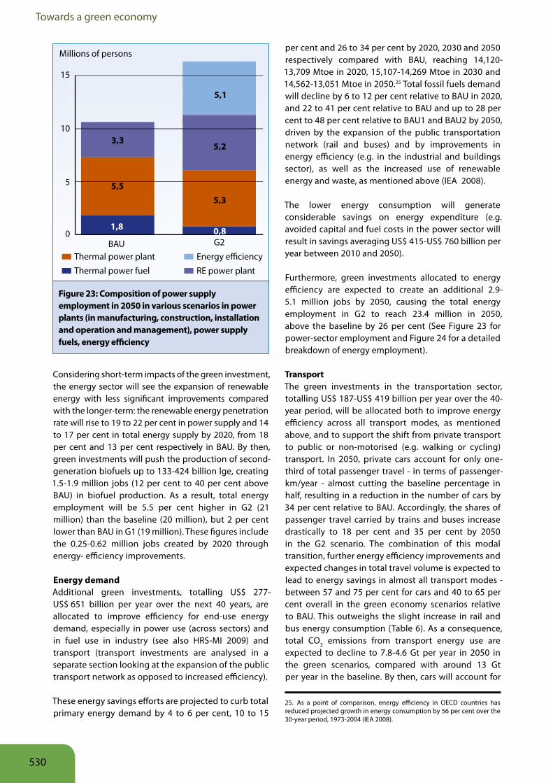
Towards a green economy
Considering short-term impacts of the green investment, the energy sector will see the expansion of renewable energy with less significant improvements compared with the longer-term: the renewable energy penetration rate will rise to 19 to 22 per cent in power supply and 14 to 17 per cent in total energy supply by 2020, from 18 per cent and 13 per cent respectively in BAU. By then, green investments will push the production of second-generation biofuels up to 133-424 billion lge, creating 1.5-1.9 million jobs (12 per cent to 40 per cent above BAU) in biofuel production. As a result, total energy employment will be 5.5 per cent higher in G2 (21 million) than the baseline (20 million), but 2 per cent lower than BAU in G1 (19 million). These figures include the 0.25-0.62 million jobs created by 2020 through energy- efficiency improvements.
Energy demandAdditional green investments, totalling US$ 277- US$ 651 billion per year over the next 40 years, are allocated to improve efficiency for end-use energy demand, especially in power use (across sectors) and in fuel use in industry (see also HRS-MI 2009) and transport (transport investments are analysed in a separate section looking at the expansion of the public transport network as opposed to increased efficiency).
These energy savings efforts are projected to curb total primary energy demand by 4 to 6 per cent, 10 to 15
per cent and 26 to 34 per cent by 2020, 2030 and 2050 respectively compared with BAU, reaching 14,120-13,709 Mtoe in 2020, 15,107-14,269 Mtoe in 2030 and 14,562-13,051 Mtoe in 2050.25 Total fossil fuels demand will decline by 6 to 12 per cent relative to BAU in 2020, and 22 to 41 per cent relative to BAU and up to 28 per cent to 48 per cent relative to BAU1 and BAU2 by 2050, driven by the expansion of the public transportation network (rail and buses) and by improvements in energy efficiency (e.g. in the industrial and buildings sector), as well as the increased use of renewable energy and waste, as mentioned above (IEA 2008).
The lower energy consumption will generate considerable savings on energy expenditure (e.g. avoided capital and fuel costs in the power sector will result in savings averaging US$ 415-US$ 760 billion per year between 2010 and 2050).
Furthermore, green investments allocated to energy efficiency are expected to create an additional 2.9-5.1 million jobs by 2050, causing the total energy employment in G2 to reach 23.4 million in 2050, above the baseline by 26 per cent (See Figure 23 for power-sector employment and Figure 24 for a detailed breakdown of energy employment).
TransportThe green investments in the transportation sector, totalling US$ 187-US$ 419 billion per year over the 40-year period, will be allocated both to improve energy efficiency across all transport modes, as mentioned above, and to support the shift from private transport to public or non-motorised (e.g. walking or cycling) transport. In 2050, private cars account for only one-third of total passenger travel - in terms of passenger-km/year - almost cutting the baseline percentage in half, resulting in a reduction in the number of cars by 34 per cent relative to BAU. Accordingly, the shares of passenger travel carried by trains and buses increase drastically to 18 per cent and 35 per cent by 2050 in the G2 scenario. The combination of this modal transition, further energy efficiency improvements and expected changes in total travel volume is expected to lead to energy savings in almost all transport modes - between 57 and 75 per cent for cars and 40 to 65 per cent overall in the green economy scenarios relative to BAU. This outweighs the slight increase in rail and bus energy consumption (Table 6). As a consequence, total CO2 emissions from transport energy use are expected to decline to 7.8-4.6 Gt per year in 2050 in the green scenarios, compared with around 13 Gt per year in the baseline. By then, cars will account for
25. As a point of comparison, energy efficiency in OECD countries has reduced projected growth in energy consumption by 56 per cent over the 30-year period, 1973-2004 (IEA 2008).
Figure 23: Composition of power supply employment in 2050 in various scenarios in power plants (in manufacturing, construction, installation and operation and management), power supply fuels, energy efficiency
BAU G20
5
10
15
RE power plant
Energy e�ciency
Thermal power fuel
Thermal power plant
5,5
3,3
5,3
0,81,8
5,2
5,1
Millions of persons
530
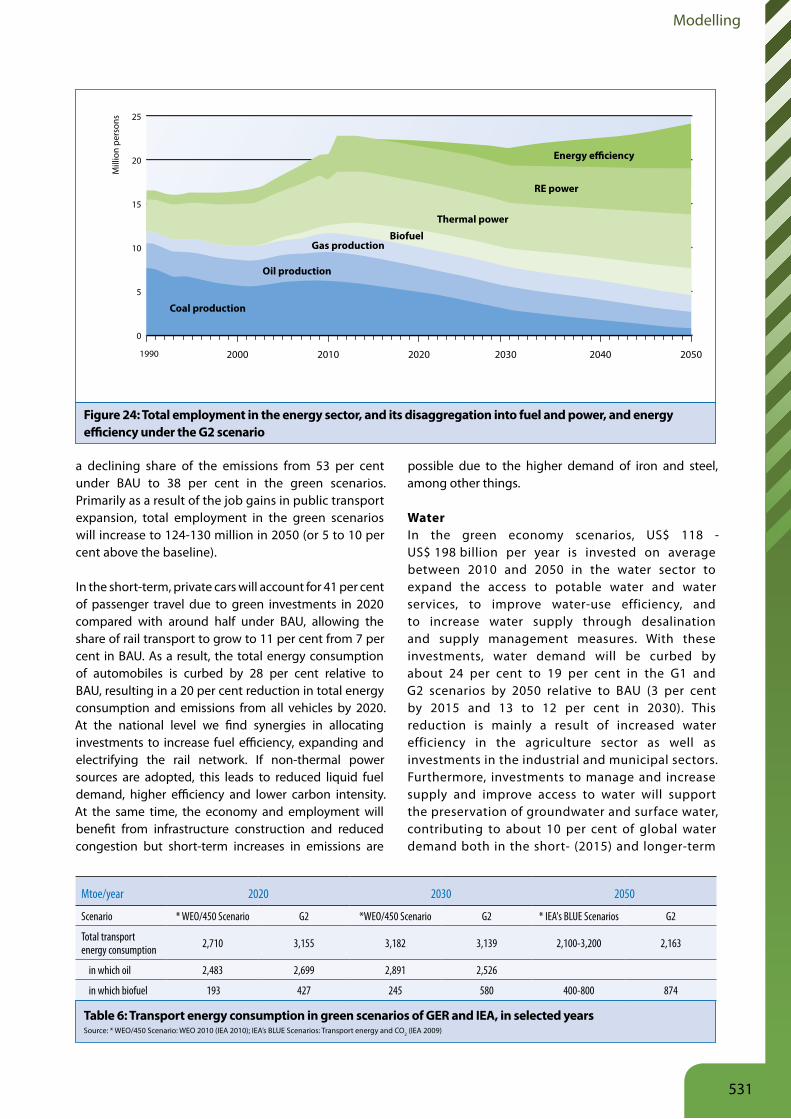
Modelling
a declining share of the emissions from 53 per cent under BAU to 38 per cent in the green scenarios. Primarily as a result of the job gains in public transport expansion, total employment in the green scenarios will increase to 124-130 million in 2050 (or 5 to 10 per cent above the baseline).
In the short-term, private cars will account for 41 per cent of passenger travel due to green investments in 2020 compared with around half under BAU, allowing the share of rail transport to grow to 11 per cent from 7 per cent in BAU. As a result, the total energy consumption of automobiles is curbed by 28 per cent relative to BAU, resulting in a 20 per cent reduction in total energy consumption and emissions from all vehicles by 2020. At the national level we find synergies in allocating investments to increase fuel efficiency, expanding and electrifying the rail network. If non-thermal power sources are adopted, this leads to reduced liquid fuel demand, higher efficiency and lower carbon intensity. At the same time, the economy and employment will benefit from infrastructure construction and reduced congestion but short-term increases in emissions are
possible due to the higher demand of iron and steel, among other things.
WaterIn the green economy scenarios, US$ 118 - US$ 198 billion per year is invested on average between 2010 and 2050 in the water sector to expand the access to potable water and water services, to improve water-use efficiency, and to increase water supply through desalination and supply management measures. With these investments, water demand will be curbed by about 24 per cent to 19 per cent in the G1 and G2 scenarios by 2050 relative to BAU (3 per cent by 2015 and 13 to 12 per cent in 2030). This reduction is mainly a result of increased water efficiency in the agriculture sector as well as investments in the industrial and municipal sectors. Furthermore, investments to manage and increase supply and improve access to water will support the preservation of groundwater and surface water, contributing to about 10 per cent of global water demand both in the short- (2015) and longer-term
Figure 24: Total employment in the energy sector, and its disaggregation into fuel and power, and energy efficiency under the G2 scenario
Mtoe/year 2020 2030 2050
Scenario * WEO/450 Scenario G2 *WEO/450 Scenario G2 * IEA's BLUE Scenarios G2
Total transport energy consumption 2,710 3,155 3,182 3,139 2,100-3,200 2,163
in which oil 2,483 2,699 2,891 2,526
in which biofuel 193 427 245 580 400-800 874
Table 6: Transport energy consumption in green scenarios of GER and IEA, in selected yearsSource: * WEO/450 Scenario: WEO 2010 (IEA 2010); IEA’s BLUE Scenarios: Transport energy and CO2 (IEA 2009)
Coal production
Oil production
Gas productionBiofuel
Thermal power
RE power
Energy e�ciency
1990 2000 2010 2020 2030 2040 2050
25
20
15
10
5
0
Mill
ion
pers
ons
531
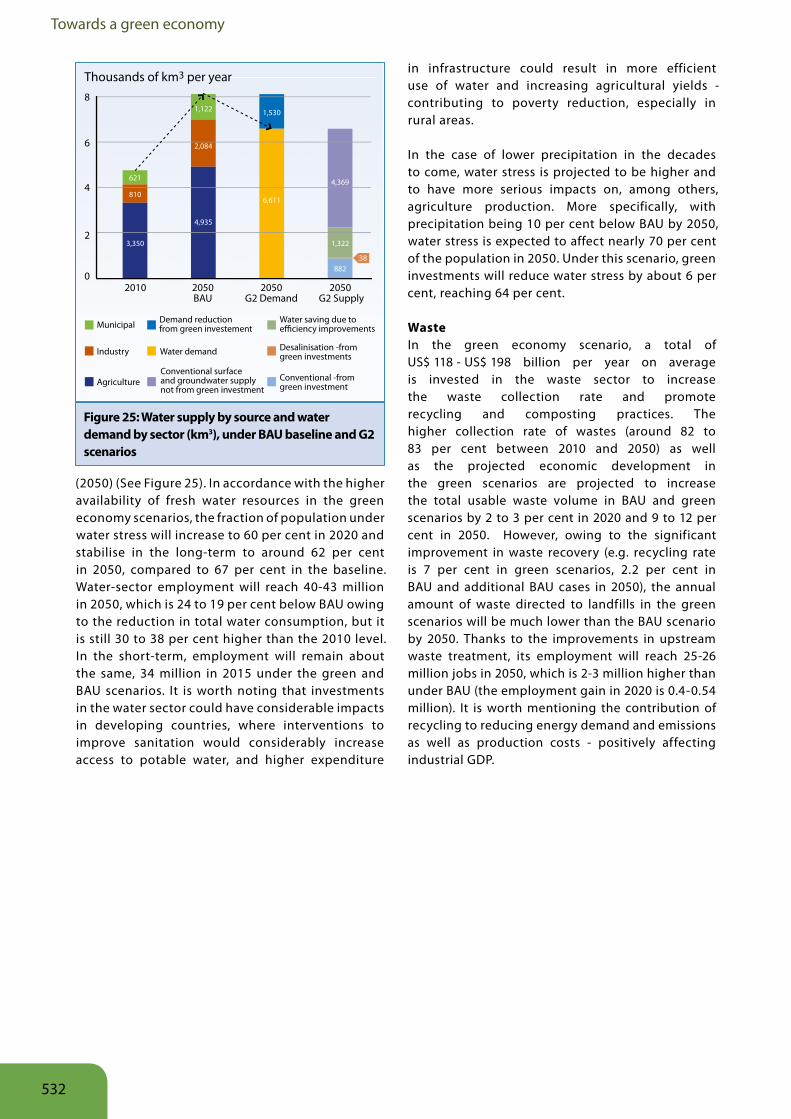
Towards a green economy
(2050) (See Figure 25). In accordance with the higher availability of fresh water resources in the green economy scenarios, the fraction of population under water stress will increase to 60 per cent in 2020 and stabilise in the long-term to around 62 per cent in 2050, compared to 67 per cent in the baseline. Water-sector employment will reach 40-43 million in 2050, which is 24 to 19 per cent below BAU owing to the reduction in total water consumption, but it is still 30 to 38 per cent higher than the 2010 level. In the short-term, employment will remain about the same, 34 million in 2015 under the green and BAU scenarios. It is worth noting that investments in the water sector could have considerable impacts in developing countries, where interventions to improve sanitation would considerably increase access to potable water, and higher expenditure
in infrastructure could result in more efficient use of water and increasing agricultural yields - contributing to poverty reduction, especially in rural areas.
In the case of lower precipitation in the decades to come, water stress is projected to be higher and to have more serious impacts on, among others, agriculture production. More specifically, with precipitation being 10 per cent below BAU by 2050, water stress is expected to affect nearly 70 per cent of the population in 2050. Under this scenario, green investments will reduce water stress by about 6 per cent, reaching 64 per cent.
WasteIn the green economy scenario, a total of US$ 118 - US$ 198 billion per year on average is invested in the waste sector to increase the waste collection rate and promote recycling and composting practices. The higher collection rate of wastes (around 82 to 83 per cent between 2010 and 2050) as well as the projected economic development in the green scenarios are projected to increase the total usable waste volume in BAU and green scenarios by 2 to 3 per cent in 2020 and 9 to 12 per cent in 2050. However, owing to the significant improvement in waste recovery (e.g. recycling rate is 7 per cent in green scenarios, 2.2 per cent in BAU and additional BAU cases in 2050), the annual amount of waste directed to landfills in the green scenarios will be much lower than the BAU scenario by 2050. Thanks to the improvements in upstream waste treatment, its employment will reach 25-26 million jobs in 2050, which is 2-3 million higher than under BAU (the employment gain in 2020 is 0.4-0.54 million). It is worth mentioning the contribution of recycling to reducing energy demand and emissions as well as production costs - positively affecting industrial GDP.
Figure 25: Water supply by source and water demand by sector (km3), under BAU baseline and G2 scenarios
2010 2050 BAU
2050 G2 Demand
2050 G2 Supply
Thousands of km3 per year8
6
4
2
0
Municipal
Industry
Agriculture
Demand reduction from green investement
Water demand
Conventional surface and groundwater supplynot from green investment
Water saving due toe�ciency improvements
Desalinisation -from green investments
Conventional -fromgreen investment
621
1,122
2,084
4,935
6,611
1,530
4,369
1,322
882
3,350
810
38
532
Modelling
6 ConclusionsThe simulation of future scenarios with an integrated cross-sectoral model highlights the characteristics of the green economy approach and provides an assessment of the global impacts of green investments, relative to BAU. These impacts are summarised below.
Undertaken at the global level, this analysis necessarily does not reflect different national or regional circumstances, which should be an area for additional work. Among other aspects, such analysis will need to pay attention to the means and ability of governments to direct investment at the scale envisaged, including necessary international financial flows.26
The projections in the additional BAU investment scenarios (BAU1 and BAU2), are for increases in GDP and employment, but accompanied by a growing depletion of natural resources. More specifically, water stress will worsen, impacting population growth, agriculture and industrial production. A larger number of vessels in the fishery sector will allow fish catch to rise in the short-term but fall in the medium- to longer-term, limited by a considerable decline of fish stocks in capture fisheries in the next 40 years. The increased use of chemical fertilisers is projected to increase yields in the agriculture sector in the short-term at the expenses of a longer-term decline of soil quality. This will require more land - converted from forest area to farmland - to feed the growing population. Moreover, the increasing use of fossil fuels projected in the additional BAU scenarios will further jeopardise energy security and tend to slow economic growth, through higher energy (especially oil) prices. As a consequence of high fossil fuel dependency and deforestation, CO2 emissions are projected to grow beyond BAU over the 40-year period. As a consequence, while GDP will still grow, its pressure on natural resources will increase, pushing our ecological footprint to over two times the available biocapacity by 2050 and atmospheric carbon concentrations to over 1,000 ppm by 2100.
In the green economy scenarios, one observes significant efficiency improvements, resource conservation and carbon mitigation, which contribute to stronger and more resilient economic growth in the medium- and long-term. The
26. Such issues are discussed in more detail in the chapters on enabling conditions and finance.
sustainable management of natural resources, resulting from a reduction in fishing capacity, a decline in deforestation, the promotion of organic fertiliser and a reduction in fossil fuel use, will allow the restoration of stocks of key natural resources, or greatly mitigate their depletion. For example, fish stocks, forestland and soil quality are estimated to increase by 64 to 106 per cent, 21 per cent and 21 to 27 per cent respectively relative to BAU by 2050, with clear benefits for the productivity of these sectors. In addition, the efficiency improvement of water and energy use in a number of sectors will considerably curb the consumption of these resources (below BAU by 34 to 50 per cent for fossil fuels and 24 to 19 per cent for water in 2050) and avoid negative consequences arising from their depletion. With increased carbon sequestration from forests, the potential sequestration from conservation agriculture (still to be estimated in detail), and the substitution of traditional energy resources with low-carbon alternatives, CO2 and GHG emissions, will be considerably lower than BAU over the next 40 years.
Increasingly decoupled from the consumption of natural resources, GDP growth under a green scenario is expected to surpass that under BAU in the medium- to long-term. Taking into account the improved maintenance of natural capital in the G1 and G2 scenarios, an adjusted measure of net domestic product would probably perform even more favourably relative to the BAU scenarios (see Box 1). Driven primarily by green investments and the subsequent push to economic development, total net direct employment in the sectors analysed in this chapter is projected to be lower than additional BAU cases in the short-term, and to then rise above all BAU scenarios in the medium to long run (2-3 per cent above BAU1 and BAU2 scenarios, respectively, and 8 to 14 per cent above BAU in 2050). When total employment is considered, the green scenarios are expected to converge to the corresponding BAU cases in the longer-term, and exceed BAU by 3 to 5 per cent in 40 years. These results point to the need for policies that recognise and manage the transition costs involved in moving towards a green economy, with a focus on an equitable distribution of costs and benefits that emerge from new opportunities.
533
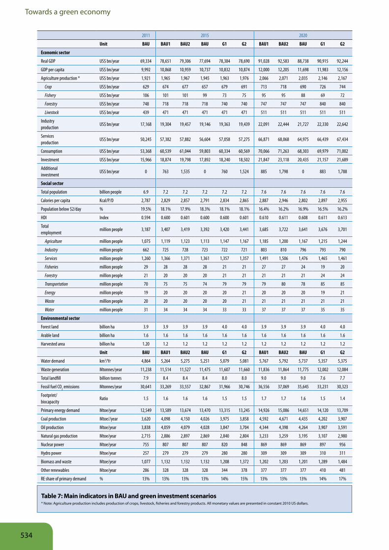
Towards a green economy
2011 2015 2020
Unit BAU BAU1 BAU2 BAU G1 G2 BAU1 BAU2 BAU G1 G2
Economic sector
Real GDP US$ bn/year 69,334 78,651 79,306 77,694 78,384 78,690 91,028 92,583 88,738 90,915 92,244
GDP per capita US$ bn/year 9,992 10,868 10,959 10,737 10,832 10,874 12,000 12,205 11,698 11,983 12,156
Agriculture production * US$ bn/year 1,921 1,965 1,967 1,945 1,963 1,976 2,066 2,071 2,035 2,146 2,167
Crop US$ bn/year 629 674 677 657 679 691 713 718 690 726 744
Fishery US$ bn/year 106 101 101 99 73 75 95 95 88 69 72
Forestry US$ bn/year 748 718 718 718 740 740 747 747 747 840 840
Livestock US$ bn/year 439 471 471 471 471 471 511 511 511 511 511
Industry production
US$ bn/year 17,168 19,304 19,457 19,146 19,363 19,439 22,091 22,444 21,727 22,330 22,642
Services production
US$ bn/year 50,245 57,382 57,882 56,604 57,058 57,275 66,871 68,068 64,975 66,439 67,434
Consumption US$ bn/year 53,368 60,539 61,044 59,803 60,334 60,569 70,066 71,263 68,303 69,979 71,002
Investment US$ bn/year 15,966 18,874 19,798 17,892 18,240 18,502 21,847 23,118 20,435 21,157 21,689
Additional investment
US$ bn/year 0 763 1,535 0 760 1,524 885 1,798 0 883 1,788
Social sector
Total population billion people 6.9 7.2 7.2 7.2 7.2 7.2 7.6 7.6 7.6 7.6 7.6
Calories per capita Kcal/P/D 2,787 2,829 2,857 2,791 2,834 2,865 2,887 2,946 2,802 2,897 2,955
Population below $2/day % 19.5% 18.1% 17.9% 18.3% 18.1% 18.1% 16.4% 16.2% 16.9% 16.5% 16.2%
HDI Index 0.594 0.600 0.601 0.600 0.600 0.601 0.610 0.611 0.608 0.611 0.613
Total employment
million people 3,187 3,407 3,419 3,392 3,420 3,441 3,685 3,722 3,641 3,676 3,701
Agriculture million people 1,075 1,119 1,123 1,113 1,147 1,167 1,185 1,200 1,167 1,215 1,244
Industry million people 662 725 728 723 722 721 803 810 796 793 790
Services million people 1,260 1,366 1,371 1,361 1,357 1,357 1,491 1,506 1,476 1,465 1,461
Fisheries million people 29 28 28 28 21 21 27 27 24 19 20
Forestry million people 21 20 20 20 21 21 21 21 21 24 24
Transportation million people 70 75 75 74 79 79 79 80 78 85 85
Energy million people 19 20 20 20 20 21 20 20 20 19 21
Waste million people 20 20 20 20 20 21 21 21 21 21 21
Water million people 31 34 34 34 33 33 37 37 37 35 35
Environmental sector
Forest land billion ha 3.9 3.9 3.9 3.9 4.0 4.0 3.9 3.9 3.9 4.0 4.0
Arable land billion ha 1.6 1.6 1.6 1.6 1.6 1.6 1.6 1.6 1.6 1.6 1.6
Harvested area billion ha 1.20 1.2 1.2 1.2 1.2 1.2 1.2 1.2 1.2 1.2 1.2
Unit BAU BAU1 BAU2 BAU G1 G2 BAU1 BAU2 BAU G1 G2
Water demand km3/Yr 4,864 5,264 5,275 5,251 5,079 5,081 5,767 5,792 5,737 5,357 5,375
Waste generation Mtonnes/year 11,238 11,514 11,527 11,475 11,607 11,660 11,836 11,864 11,775 12,002 12,084
Total landfill billion tonnes 7.9 8.4 8.4 8.4 8.0 8.0 9.0 9.0 9.0 7.6 7.7
Fossil fuel CO2 emissions Mtonnes/year 30,641 33,269 33,557 32,867 31,966 30,746 36,556 37,069 35,645 33,231 30,323
Footprint/ biocapacity
Ratio 1.5 1.6 1.6 1.6 1.5 1.5 1.7 1.7 1.6 1.5 1.4
Primary energy demand Mtoe/year 12,549 13,589 13,674 13,470 13,315 13,245 14,926 15,086 14,651 14,120 13,709
Coal production Mtoe//year 3,620 4,098 4,150 4,026 3,975 3,858 4,592 4,671 4,435 4,202 3,907
Oil production Mtoe/year 3,838 4,059 4,079 4,028 3,847 3,704 4,344 4,398 4,264 3,907 3,591
Natural gas production Mtoe/year 2,715 2,886 2,897 2,869 2,840 2,804 3,233 3,259 3,195 3,107 2,980
Nuclear power Mtoe/year 755 807 807 807 820 848 869 869 869 897 956
Hydro power Mtoe/year 257 279 279 279 280 280 309 309 309 310 311
Biomass and waste Mtoe/year 1,077 1,132 1,132 1,132 1,208 1,372 1,202 1,203 1,201 1,289 1,484
Other renewables Mtoe/year 286 328 328 328 344 378 377 377 377 410 481
RE share of primary demand % 13% 13% 13% 13% 14% 15% 13% 13% 13% 14% 17%
Table 7: Main indicators in BAU and green investment scenarios* Note: Agriculture production includes production of crops, livestock, fisheries and forestry products. All monetary values are presented in constant 2010 US dollars.
534
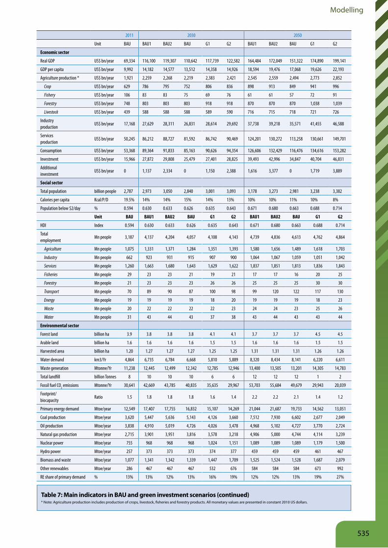
Modelling
2011 2030 2050
Unit BAU BAU1 BAU2 BAU G1 G2 BAU1 BAU2 BAU G1 G2
Economic sector
Real GDP US$ bn/year 69,334 116,100 119,307 110,642 117,739 122,582 164,484 172,049 151,322 174,890 199,141
GDP per capita US$ bn/year 9,992 14,182 14,577 13,512 14,358 14,926 18,594 19,476 17,068 19,626 22,193
Agriculture production * US$ bn/year 1,921 2,259 2,268 2,219 2,383 2,421 2,545 2,559 2,494 2,773 2,852
Crop US$ bn/year 629 786 795 752 806 836 898 913 849 941 996
Fishery US$ bn/year 106 83 83 75 69 76 61 61 57 72 91
Forestry US$ bn/year 748 803 803 803 918 918 870 870 870 1,038 1,039
Livestock US$ bn/year 439 588 588 588 589 590 716 715 718 721 726
Industry production
US$ bn/year 17,168 27,629 28,311 26,831 28,614 29,692 37,738 39,218 35,571 41,455 46,588
Services production
US$ bn/year 50,245 86,212 88,727 81,592 86,742 90,469 124,201 130,272 113,258 130,661 149,701
Consumption US$ bn/year 53,368 89,364 91,833 85,163 90,626 94,354 126,606 132,429 116,476 134,616 153,282
Investment US$ bn/year 15,966 27,872 29,808 25,479 27,401 28,825 39,493 42,996 34,847 40,704 46,831
Additional investment
US$ bn/year 0 1,137 2,334 0 1,150 2,388 1,616 3,377 0 1,719 3,889
Social sector
Total population billion people 2,787 2,973 3,050 2,840 3,001 3,093 3,178 3,273 2,981 3,238 3,382
Calories per capita Kcal/P/D 19.5% 14% 14% 15% 14% 13% 10% 10% 11% 10% 8%
Population below $2/day % 0.594 0.630 0.633 0.626 0.635 0.643 0.671 0.680 0.663 0.688 0.714
Unit BAU BAU1 BAU2 BAU G1 G2 BAU1 BAU2 BAU G1 G2
HDI Index 0.594 0.630 0.633 0.626 0.635 0.643 0.671 0.680 0.663 0.688 0.714
Total employment
Mn people 3,187 4,137 4,204 4,057 4,108 4,143 4,739 4,836 4,613 4,762 4,864
Agriculture Mn people 1,075 1,331 1,371 1,284 1,351 1,393 1,580 1,656 1,489 1,618 1,703
Industry Mn people 662 923 931 915 907 900 1,064 1,067 1,059 1,051 1,042
Services Mn people 1,260 1,663 1,680 1,643 1,629 1,622 1,837 1,851 1,813 1,836 1,843
Fisheries Mn people 29 23 23 21 19 21 17 17 16 20 25
Forestry Mn people 21 23 23 23 26 26 25 25 25 30 30
Transport Mn people 70 89 90 87 100 98 99 120 122 117 130
Energy Mn people 19 19 19 19 18 20 19 19 19 18 23
Waste Mn people 20 22 22 22 22 23 24 24 23 25 26
Water Mn people 31 43 44 43 37 38 43 44 43 43 44
Environmental sector
Forest land billion ha 3.9 3.8 3.8 3.8 4.1 4.1 3.7 3.7 3.7 4.5 4.5
Arable land billion ha 1.6 1.6 1.6 1.6 1.5 1.5 1.6 1.6 1.6 1.5 1.5
Harvested area billion ha 1.20 1.27 1.27 1.27 1.25 1.25 1.31 1.31 1.31 1.26 1.26
Water demand km3/Yr 4,864 6,735 6,784 6,668 5,810 5,889 8,320 8,434 8,141 6,220 6,611
Waste generation Mtonne/Yr 11,238 12,445 12,499 12,342 12,785 12,946 13,400 13,505 13,201 14,305 14,783
Total landfill billion Tonnes 8 10 10 10 6 6 12 12 12 1 2
Fossil fuel CO2 emissions Mtonne/Yr 30,641 42,669 43,785 40,835 35,635 29,967 53,703 55,684 49,679 29,943 20,039
Footprint/ biocapacity
Ratio 1.5 1.8 1.8 1.8 1.6 1.4 2.2 2.2 2.1 1.4 1.2
Primary energy demand Mtoe/year 12,549 17,407 17,755 16,832 15,107 14,269 21,044 21,687 19,733 14,562 13,051
Coal production Mtoe/year 3,620 5,447 5,636 5,143 4,126 3,660 7,512 7,930 6,602 2,677 2,049
Oil production Mtoe/year 3,838 4,910 5,019 4,726 4,026 3,478 4,968 5,102 4,727 3,770 2,724
Natural gas production Mtoe/year 2,715 3,901 3,951 3,816 3,578 3,218 4,906 5,000 4,744 4,114 3,239
Nuclear power Mtoe/year 755 968 968 968 1,024 1,151 1,089 1,089 1,089 1,179 1,500
Hydro power Mtoe/year 257 373 373 373 374 377 459 459 459 461 467
Biomass and waste Mtoe/year 1,077 1,341 1,342 1,339 1,447 1,709 1,525 1,524 1,528 1,687 2,079
Other renewables Mtoe/year 286 467 467 467 532 676 584 584 584 673 992
RE share of primary demand % 13% 13% 12% 13% 16% 19% 12% 12% 13% 19% 27%
Table 7: Main indicators in BAU and green investment scenarios (continued)* Note: Agriculture production includes production of crops, livestock, fisheries and forestry products. All monetary values are presented in constant 2010 US dollars.
535
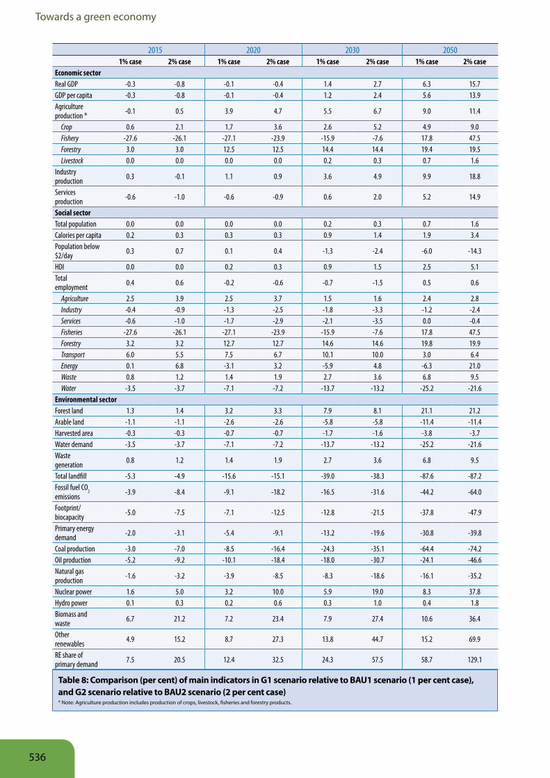
Towards a green economy
Table 8: Comparison (per cent) of main indicators in G1 scenario relative to BAU1 scenario (1 per cent case), and G2 scenario relative to BAU2 scenario (2 per cent case)* Note: Agriculture production includes production of crops, livestock, fisheries and forestry products.
2015 2020 2030 20501% case 2% case 1% case 2% case 1% case 2% case 1% case 2% case
Economic sectorReal GDP -0.3 -0.8 -0.1 -0.4 1.4 2.7 6.3 15.7GDP per capita -0.3 -0.8 -0.1 -0.4 1.2 2.4 5.6 13.9Agriculture production * -0.1 0.5 3.9 4.7 5.5 6.7 9.0 11.4
Crop 0.6 2.1 1.7 3.6 2.6 5.2 4.9 9.0 Fishery -27.6 -26.1 -27.1 -23.9 -15.9 -7.6 17.8 47.5 Forestry 3.0 3.0 12.5 12.5 14.4 14.4 19.4 19.5 Livestock 0.0 0.0 0.0 0.0 0.2 0.3 0.7 1.6Industry production 0.3 -0.1 1.1 0.9 3.6 4.9 9.9 18.8
Services production -0.6 -1.0 -0.6 -0.9 0.6 2.0 5.2 14.9
Social sectorTotal population 0.0 0.0 0.0 0.0 0.2 0.3 0.7 1.6Calories per capita 0.2 0.3 0.3 0.3 0.9 1.4 1.9 3.4Population below $2/day 0.3 0.7 0.1 0.4 -1.3 -2.4 -6.0 -14.3
HDI 0.0 0.0 0.2 0.3 0.9 1.5 2.5 5.1Total employment 0.4 0.6 -0.2 -0.6 -0.7 -1.5 0.5 0.6
Agriculture 2.5 3.9 2.5 3.7 1.5 1.6 2.4 2.8 Industry -0.4 -0.9 -1.3 -2.5 -1.8 -3.3 -1.2 -2.4 Services -0.6 -1.0 -1.7 -2.9 -2.1 -3.5 0.0 -0.4 Fisheries -27.6 -26.1 -27.1 -23.9 -15.9 -7.6 17.8 47.5 Forestry 3.2 3.2 12.7 12.7 14.6 14.6 19.8 19.9 Transport 6.0 5.5 7.5 6.7 10.1 10.0 3.0 6.4 Energy 0.1 6.8 -3.1 3.2 -5.9 4.8 -6.3 21.0 Waste 0.8 1.2 1.4 1.9 2.7 3.6 6.8 9.5 Water -3.5 -3.7 -7.1 -7.2 -13.7 -13.2 -25.2 -21.6Environmental sectorForest land 1.3 1.4 3.2 3.3 7.9 8.1 21.1 21.2Arable land -1.1 -1.1 -2.6 -2.6 -5.8 -5.8 -11.4 -11.4Harvested area -0.3 -0.3 -0.7 -0.7 -1.7 -1.6 -3.8 -3.7Water demand -3.5 -3.7 -7.1 -7.2 -13.7 -13.2 -25.2 -21.6Waste generation 0.8 1.2 1.4 1.9 2.7 3.6 6.8 9.5
Total landfill -5.3 -4.9 -15.6 -15.1 -39.0 -38.3 -87.6 -87.2Fossil fuel CO
2 emissions -3.9 -8.4 -9.1 -18.2 -16.5 -31.6 -44.2 -64.0
Footprint/ biocapacity -5.0 -7.5 -7.1 -12.5 -12.8 -21.5 -37.8 -47.9
Primary energy demand -2.0 -3.1 -5.4 -9.1 -13.2 -19.6 -30.8 -39.8
Coal production -3.0 -7.0 -8.5 -16.4 -24.3 -35.1 -64.4 -74.2Oil production -5.2 -9.2 -10.1 -18.4 -18.0 -30.7 -24.1 -46.6Natural gas production -1.6 -3.2 -3.9 -8.5 -8.3 -18.6 -16.1 -35.2
Nuclear power 1.6 5.0 3.2 10.0 5.9 19.0 8.3 37.8Hydro power 0.1 0.3 0.2 0.6 0.3 1.0 0.4 1.8Biomass and waste 6.7 21.2 7.2 23.4 7.9 27.4 10.6 36.4
Other renewables 4.9 15.2 8.7 27.3 13.8 44.7 15.2 69.9
RE share of primary demand 7.5 20.5 12.4 32.5 24.3 57.5 58.7 129.1
536
Modelling
Annex 1. Technical specifications of the Threshold 21 (T21) World modelFinding that currently available national and global planning models are either too detailed or narrowly focused, and perhaps too decision oriented and prescriptive, this study proposes an approach that a) extends and advances the policy analysis carried out with existing tools by accounting for the dynamic complexity embedded in the systems studied, and b) facilitates the investigation and understanding of the relations existing between energy and society, economy and the environment. This is crucial, since understanding the characteristics of real systems, feedback, delays and non-linearity is fundamental for the correct representation of structures, whose behaviour is outside their normal operating range (Sterman 2000; see also Figure 1). The inclusion of cross-sectoral relationships - social, economic and environmental - allows for a wider analysis of the implication of policies by identifying potential side effects or longer-term bottlenecks for development. In other words, a policy can have very positive impacts for certain sectors and create issues for others. Also, successful policies in the longer-term may have negative short-term impacts, for which mitigating actions may be designed and implemented.
As indicated earlier, the approach proposed uses System Dynamics as its foundation and incorporates various methodologies, such as optimisation (in the energy sector) and econometrics (in the economic sectors). The integrated global model is used to: (1) provide an integrated analysis and evaluation of investment choices; (2) generate projections of future developments (though acknowledging that long-term accurate projection cannot easily be produced, even when simulating a large number of endogenous key variables (Sarewitz 2000); (3) increase the understanding of the relations underlying the system analysed; and (4) and bring consistency to models.
The Threshold21 (T21) World model (T21-World) is structured to analyse medium- long-term development issues. The model integrates in a single framework the economic, the social, and the environmental aspects of development planning. T21-World modelling structure includes both monetary and physical indicators, to fully analyse the impacts of investments on natural resources, low-carbon development, economic growth and job creation. Key characteristics of the model are highlighted below.
Boundaries: Variables that are considered an essential part of the development mechanisms, object of the research, are endogenously calculated. For example, GDP and its main determinants, population and its main determinants, and the demand and supply of natural resources are endogenously determined. Variables that have an important influence on the issues are analysed, but those that are only weakly influenced by the issues analysed or that cannot be endogenously estimated with confidence are exogenously represented.
Granularity: The T21-World model presented in this chapter is a global model, with no regional or national disaggregation; although, the model is routinely developed for specific countries, and is applicable at other scales such as communities.27 Nonetheless, the main social, economic and environmental variables of T21-World are disaggregated in considerable detail. For example, population is divided into 82 age-cohorts and 2 genders, and the age-gender distinction is used in most social indicators; production is divided into industry, services and agriculture, this last further divided into crops, fishery, animal husbandry and forestry; land is divided into forest, agriculture, fallow, urban and desert. Finally, given its level of aggregation, the model is generally based on global average values for variables such as unit costs and prices.
Time horizon: T21-World is built to analyse medium- to long-term development issues. The time horizon for simulation begins in 1970 and extends to 2050. Beginning the simulation in 1970 ensures that, in most cases, the historical patterns of behaviour characterising the issues being investigated can be replicated by the model.
Modules, sectors and spheres: T21-World is a relatively large model, which includes more than 200 stock variables and several thousand feedback loops. Because of its size and level of complexity, the structure of the model has been reorganised into smaller logical units, called modules. A module is a structure, whose internal mechanisms can be understood in isolation from the rest of the model.28 The 80 modules comprising T21-
27. As it is emphasised later on in the text, although it is possible to understand the internal mechanism of a specific module in isolation from the rest of the model, the fully understanding of its functioning and relevance requires studying its role in the whole model’s structure.
28. For more information, see Bassi and Baer (2009), Bassi and Yudken (2009), Bassi and Shilling (2010), Bassi et al. (2009a, 2009b, 2010), Magnoni and Bassi (2009), Pedercini and Barney (In Press), Yudken and Bassi (2009).
537
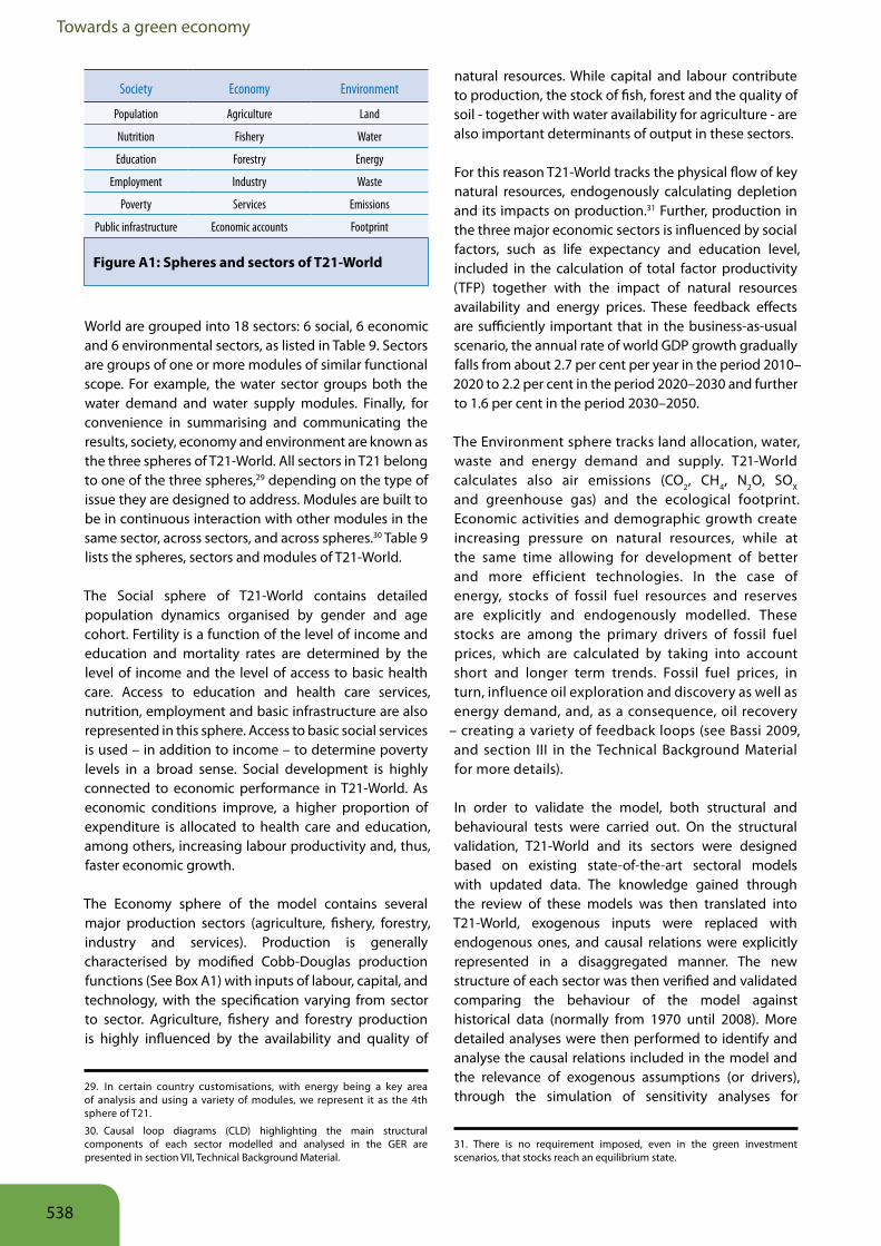
Towards a green economy
World are grouped into 18 sectors: 6 social, 6 economic and 6 environmental sectors, as listed in Table 9. Sectors are groups of one or more modules of similar functional scope. For example, the water sector groups both the water demand and water supply modules. Finally, for convenience in summarising and communicating the results, society, economy and environment are known as the three spheres of T21-World. All sectors in T21 belong to one of the three spheres,29 depending on the type of issue they are designed to address. Modules are built to be in continuous interaction with other modules in the same sector, across sectors, and across spheres.30 Table 9 lists the spheres, sectors and modules of T21-World.
The Social sphere of T21-World contains detailed population dynamics organised by gender and age cohort. Fertility is a function of the level of income and education and mortality rates are determined by the level of income and the level of access to basic health care. Access to education and health care services, nutrition, employment and basic infrastructure are also represented in this sphere. Access to basic social services is used – in addition to income – to determine poverty levels in a broad sense. Social development is highly connected to economic performance in T21-World. As economic conditions improve, a higher proportion of expenditure is allocated to health care and education, among others, increasing labour productivity and, thus, faster economic growth.
The Economy sphere of the model contains several major production sectors (agriculture, fishery, forestry, industry and services). Production is generally characterised by modified Cobb-Douglas production functions (See Box A1) with inputs of labour, capital, and technology, with the specification varying from sector to sector. Agriculture, fishery and forestry production is highly influenced by the availability and quality of
29. In certain country customisations, with energy being a key area of analysis and using a variety of modules, we represent it as the 4th sphere of T21.
30. Causal loop diagrams (CLD) highlighting the main structural components of each sector modelled and analysed in the GER are presented in section VII, Technical Background Material.
natural resources. While capital and labour contribute to production, the stock of fish, forest and the quality of soil - together with water availability for agriculture - are also important determinants of output in these sectors.
For this reason T21-World tracks the physical flow of key natural resources, endogenously calculating depletion and its impacts on production.31 Further, production in the three major economic sectors is influenced by social factors, such as life expectancy and education level, included in the calculation of total factor productivity (TFP) together with the impact of natural resources availability and energy prices. These feedback effects are sufficiently important that in the business-as-usual scenario, the annual rate of world GDP growth gradually falls from about 2.7 per cent per year in the period 2010–2020 to 2.2 per cent in the period 2020–2030 and further to 1.6 per cent in the period 2030–2050.
The Environment sphere tracks land allocation, water, waste and energy demand and supply. T21-World calculates also air emissions (CO2, CH4, N2O, SOX and greenhouse gas) and the ecological footprint. Economic activities and demographic growth create increasing pressure on natural resources, while at the same time allowing for development of better and more efficient technologies. In the case of energy, stocks of fossil fuel resources and reserves are explicitly and endogenously modelled. These stocks are among the primary drivers of fossil fuel prices, which are calculated by taking into account short and longer term trends. Fossil fuel prices, in turn, influence oil exploration and discovery as well as energy demand, and, as a consequence, oil recovery
– creating a variety of feedback loops (see Bassi 2009, and section III in the Technical Background Material for more details).
In order to validate the model, both structural and behavioural tests were carried out. On the structural validation, T21-World and its sectors were designed based on existing state-of-the-art sectoral models with updated data. The knowledge gained through the review of these models was then translated into T21-World, exogenous inputs were replaced with endogenous ones, and causal relations were explicitly represented in a disaggregated manner. The new structure of each sector was then verified and validated comparing the behaviour of the model against historical data (normally from 1970 until 2008). More detailed analyses were then performed to identify and analyse the causal relations included in the model and the relevance of exogenous assumptions (or drivers), through the simulation of sensitivity analyses for
31. There is no requirement imposed, even in the green investment scenarios, that stocks reach an equilibrium state.
Figure A1: Spheres and sectors of T21-World
Society Economy Environment
Population Agriculture Land
Nutrition Fishery Water
Education Forestry Energy
Employment Industry Waste
Poverty Services Emissions
Public infrastructure Economic accounts Footprint
538
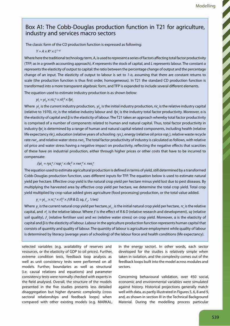
Modelling
selected variables (e.g. availability of reserves and resources, or the elasticity of GDP to oil prices). Further, extreme condition tests, feedback loop analysis as well as unit consistency tests were performed on all models. Further, boundaries as well as structural (i.e. causal relations and equations) and parameter consistency tests were normally checked with experts in the field analysed. Overall, the structure of the models presented in the five studies presents less detailed disaggregation but higher dynamic complexity (cross sectoral relationships and feedback loops) when compared with other existing models (e.g. MARKAL,
in the energy sector). In other words, each sector developed for the studies is relatively simple when taken in isolation, and the complexity comes out of the feedback loops built into the model across modules and sectors.
Concerning behavioural validation, over 450 social, economic and environmental variables were simulated against history. Historical projections generally match well with data, as partly illustrated in Figures 5, 6, 8 and 9, and, as shown in section III in the Technical Background Material. During the modelling process particular
Box A1: The Cobb-Douglas production function in T21 for agriculture, industry and services macro sectors
The classic form of the CD production function is expressed as following:
Y = A × Kα × L(1-α)
Where here the traditional technology term, A, is used to represent a series of factors affecting total factor productivity (TFP; as in a growth accounting approach), K represents the stock of capital, and L represents labour. The constant α represents the elasticity of output to capital: the ratio between the percentage change of output and the percentage change of an input. The elasticity of output to labour is set to 1-α, assuming that there are constant returns to scale (the production function is thus first order, homogeneous). In T21 the standard CD production function is transformed into a more transparent algebraic form, and TFP is expanded to include several different elements.
The equation used to estimate industry production is as shown below:
yit = yi0 × rictα × rilt
β × fpit
Where yit is the current industry production, yi0 is the initial industry production, rict is the relative industry capital (relative to 1970), ricl is the relative industry labour and fpit is the industry total factor productivity. Moreover, α is the elasticity of capital and β is the elasticity of labour. The T21 takes an approach whereby total factor productivity is comprised of a number of components related to human and natural capital. Thus, total factor productivity in industry fpit is determined by a range of human and natural capital related components, including health (relative life expectancy rlet), education (relative years of schooling ryst), energy (relative oil price ropt ), relative waste recycle rate rwrt , and relative water stress rwst. The total factor productivity of industry is calculated as follows, with relative oil price and water stress having a negative impact on productivity, reflecting the negative effects that scarcities of these have on industrial production, either through higher prices or other costs that have to be incurred to compensate:
ƒpit = rystα / ropt
c × rletβ × rwrt
d × rwste
The equation used to estimate agricultural production is defined in terms of yield, still determined by a transformed Cobb-Douglas production function, uses different inputs for TFP. The equation below is used to estimate natural yield per hectare. Effective crop yield is the natural crop yield per hectare minus yield lost due to pest diseases. By multiplying the harvested area by effective crop yield per hectare, we determine the total crop yield. Total crop yield multiplied by crop value added gives agriculture (food processing) production, or the total value added.
yt = yit-1 × rctα × rlt
β × ƒ(R & D, sq, ƒt, , 1/ws)
Where yt is the current natural crop yield per hectare, yit-1 is the initial natural crop yield per hectare, rct is the relative
capital, and rlt is the relative labour. Where ƒ is the effect of R & D (relative research and development), sq (relative
soil quality), ƒt (relative fertiliser use) and ws (relative water stress) on crop yield. Moreover, α is the elasticity of capital and β is the elasticity of labour. Labour in the agriculture production function represents human capital that consists of quantity and quality of labour. The quantity of labour is agriculture employment while quality of labour is determined by literacy (average years of schooling) of the labour force and health conditions (life expectancy).
539
Towards a green economy
emphasis was given to the analysis of the performance of aggregated indicators, and details were added and more carefully addressed in the models of the specific sectors analysed in the GER - where adding granularity was useful to provide insights on the impact of selected investments. Furthermore, future projections were compared with those from other organisations, as shown in section III of the Technical Background Material, including among others, the IEA, FAO, World Bank, UNIDO, United Nations Population Division, United Nations Statistics Divsion, and McKinsey & Company.
Finally, it is worth mentioning at the outset that the model has several limitations relative to the breadth of the GER. T21-World is a global model (with no regional or national disaggregation, and no explicit representation of trade) that focuses on medium- to longer term trends. In addition, T21-World includes only a limited amount of feedbacks linking GHG emissions to health and economic activity, and accounts for a limited number of natural resources (e.g. details on stock of non-fuel minerals are not included in the model). Further, the model does not quantify biodiversity and does not fully capture a number of important features of the labour market (while labour force, employment figures and income are calculated endogenously, disaggregated real wages by sector are not estimated and the quality of work, or “decent work”, could not be determined with confidence). Finally, the capital and financial markets are not specifically modelled, and T21-World uses a supply-side approach to production, although in many cases both demand and supply are calculated at the sectoral level.32 33
32. Other existing models used to support medium- to longer term planning exercises and analysis face similar issues, and often have very narrow boundaries compared to T21-World. OECD models employed to project scenarios presented in their environmental outlook do not explicitly account for the labour market and unemployment, and World Bank budgetary frameworks often do not single out capital and financial markets. Sectoral models - normally based on case studies - exist, but there is little agreement on the extent to which these relate to other sectors and dynamic projections of future trends are normally missing. More details on model specifications are provided in various sections of the Technical Background Material.
33. More information on T21, and several customizations and country applications can be found at www.millennium-institute.org. Selected publications include: Bassi (2010a, 2011), Bassi and Baer (2009), Bassi and Yudken, (2009, Forthcoming), Bassi and Shilling (2010), Bassi et al. (2009a, 2009b, 2010), Cimren et al. (2010), Magnoniand Bassi (2009), Yudken and Bassi (2009).
540
Modelling
ReferencesAssociation for the Study of Peak Oil and Gas ASPO-USA. “Peak Oil
Basics”. Available at: www.aspousa.org/index.php/peak-oil/peak-oil-202/. Badiou, A. (2000). “Ethics; An Essay on the Understanding of Evil.”,
translated by Peter Hallward. New York, Verso.Barlas, Y. (1996). “Formal Aspects of Model Validity and Validation
in System Dynamics.” System Dynamics Review.Bassi, A.M., (2010a). “Evaluating the use of an integrated approach
to support energy and climate policy formulation and evaluation”, Energies 3(9):1604-1621. doi:10.3390/en3091604
Bassi, A.M. (2011). “A Context-Inclusive Approach to Support Energy Policy Formulation and Evaluation”. Regional Environmental Change, 11(2), Page 285-295. DOI 10.1007/s10113-010-0139-z
Bassi, A.M. (2009). An Integrated Approach to Support Energy Policy Formulation and Evaluation. PhD Dissertation, System Dynamics Group, Department of Geography, University of Bergen, Norway. 2009. ISBILLION: 978-82-308-0908-2.
Bassi, A.M. (2010b). “Reflections on the Validity of System Dynamics Integrated Simulation Models: the case of T21 and MCM.” Currently submitted to Sustainability.
Bassi, A.M., Baer, A.E. (2009). “Quantifying Cross-Sectoral Impacts of Investments in Climate Change Mitigation in Ecuador.” Energy for Sustainable Development, 13(2009)116-123.
Bassi, A.M., J.S. Yudken (Forthcoming). “Climate Policy and Energy-Intensive Manufacturing: A Comprehensive Analysis of the Effectiveness of Cost Mitigation Provisions in the American Energy and Security Act of 2009”. Energy Policy, doi:10.1016/j.enpol.2011.06.023
Bassi, A.M., and Yudken, J.S. (2009). “Potential Challenges Faced by the U.S. Chemicals Industry Under a Carbon Policy.” Sustainability, 1(2009)592-611. Special issue on “Energy Policy and Sustainability”.
Bassi, A.M., and Shilling, J.D. (2010). “Informing the US Energy Policy Debate with Threshold 21.” Technological Forecasting & Social Change, 77 (2010) 396–410.
Bassi, A.M., Harrison J., Mistry, R. (2009a). “Using an Integrated Participatory Modelling Approach to Assess Water Management Options and Support Community Conversations on Maui.” Sustainability, 1(4), 1331-1348. Special issue on “Sustainable Water Management”.
Bassi, A.M., Schoenberg, W., Powers, R. (2010). “An integrated approach to energy prospects for North America and the Rest of the World.” Energy Economics, 32 (2010) 30–42.
Bassi, A.M., Z. Tan and S. Goss, (2010). “An Integrated Assessment of Investments to Improve Global Water Sustainability”. Water, 2(4), 726-741. doi:10.3390/w2040726
Bassi, A.M., Yudken, J.S., Ruth, M. (2009b). Climate policy impacts on the competitiveness of energy-intensive manufacturing sectors.
“Energy Policy” 37(2009)3052–3060Bio Economic Research Associates BIO-ERA. (February 2009).
“U.S. Economic Impact of Advanced Biofuels Production: Perspectives to 2030.”
Brown, S. P. A., and Huntington, H. G. (2008). “Energy Security and Climate Change Protection: Complementarity or Tradeoff?” Energy Policy, (2008) Vol. 36, No. 9.
Bussolo, M., Medvedev, D. (2007). “Challenges to MDG achievement in low income countries: lessons from Ghana and Honduras”. World Bank Policy Research Working Paper 4383, Washington DC.
Cimren, E., A.M. Bassi, J. Fiksel, (2010). “T21-Ohio, a System Dynamics Approach to Policy Assessment for Sustainable Development: A Waste to Profit Case Study.” Sustainability 2(9), 2814-2832. doi:10.3390/su2092814
CNA Corporation (2007). “National Security and the Threat of Climate Change”. Alexandria, VA.
DeGeus, A.P. (1992). “Modelling to Predict or to Learn?” European Journal of Operational Research, 59(1), p. 1-5.
Dreyfus, H. (2001). On the Internet: Thinking in Action. Routledge Press.
Evaert, L., Garcia-Pinto, F., and Venutre, J. (1990). A RMSM-X model for Turkey, Volume 1. Policy, Research, and External Affairs working paper no. WPS 486, The World Bank.
Fair, R. C. (1993). “Testing Macroeconometric Models”. The American Economic Review, 83(2): 287-293.
Fishbone, L.G., Giesen, G., Goldstein, G., Hymmen, H. A., Stocks, K. J., Vos, H., Wilde, D., Zöcher, R., Balzer, C., Abilock, H. (1983). User’s Guide for MARKAL. IEA Energy Technology Systems Analysis Programme, Upton, NY.
Food and Agriculture Organization of the United Nations FAO (2008). The State of World Fisheries and Aquaculture, 2008. Rome.
Food and Agriculture Organization of the United Nations FAO (2009). The State of World’s Forests, 2009. Rome.
Food and Agriculture Organization of the United Nations FAO (2009). World agriculture: Towards 2030/2050. Rome.
Food and Agriculture Organization of the United Nations FAO (2010). “FAOSTAT”. Rome.
Forrester, J. W. (1961). Industrial Dynamics. Productivity Press, Cambridge, MA.
Forrester, J. W. (2002). Road Maps: A Guide to Learning System Dynamics. System Dynamics Group, Sloan School of Management, MIT, Cambridge, MA.
Forrester, J. W. (2008). System Dynamics – The Next Fifty Years. System Dynamics Review.
Global Footprint Network (GFN). Available at: www.footprintnetwork.org/en/index.php/GFN .
High Road Strategies and Millennium Institute HRS-MI (2009). “Climate Policy and Energy - Intensive Manufacturing: the Competitiveness Impacts of the American Energy and Security Act of 2009”. Arlington, VA.
Howarth, R. B. and Monahan, P.A. (1996). “Economics, Ethics and Climate Policy: Framing the Debate”. Global and Planetary Change, Vol. 11, No. 4, p. 187-199.
Intergovernmental Panel on Climate Change IPCC (2007). “Fourth Assessment Report (AR4)”. Geneva.
International Energy Agency IEA. (2004). World Energy Outlook 2004. Annex C – World Energy Model. Paris.
International Energy Agency IEA. (2008). Energy Technology Perspectives (ETP) 2008. Paris.
International Energy Agency IEA. (2009). Transport, Energy and CO2: Moving Toward Sustainability. Paris.
International Energy Agency IEA. (2009). World Energy Outlook 2009. Paris.
International Energy Agency IEA. (2010). Energy Technology Perspectives (ETP) 2010. Paris.
International Energy Agency IEA. (2010). World Energy Outlook 2010. Paris.International Energy Agency IEA, and OECD. (2010). Sustainable
Production of Second-Generation Biofuels. Paris.International Labour Organization ILO. (January 2009). Global
Employment Trends Report 2009. Geneva.International Institute for Applied Systems Analysis IIASA. (2001).
Model MESSAGE. Command Line User Manual, Version 0.18.International Institute for Applied Systems Analysis IIASA. (2002).
“Achieving a Sustainable Energy System.”Haque, N.U., Khan, M.S., and Montiel, P. (1990). “Adjustment with
Growth: Relating the Analytical Approaches of the IMF and the World Bank.” Journal of Development Economics, 32: 155–79.
Lewis, W.A. (2003/1966). Development Planning: The Essentials of Economic Policy. New York, Routledge.
Goldstein, G., Loulou, R., Noble, K. (2004). “Documentation for the MARKAL Family of Models.” IEA Energy Technology Systems Analysis Programmeme.
Magnoni, S. and Bassi, A.M. (2009). “Creating Synergies from Renewable Energy Investments, a Community Success Story on Lolland, Denmark.” Energies 2009, 2(4), 1151-1169. Special issue on
“Energy Economics”.McKinsey & Company and 2030 Water Resources Group. (2009).
Charting Our Water Future. Washington, DC.Meadows, D. (1980). “The Unavoidable A Priori.” Excerpt from
Randers. Elements of the System Dynamics Method.Millennium Institute. (2005). “Threshold 21 (T21) Overview.”
Arlington, VA.
541
Towards a green economy
Morecroft, J.D.W. (1992). “Executive Knowledge, Models and Learning.” European Journal of Operational Research, 59(1), p. 70-74.
Müller, A. and Davis, J. S. (2009) “Reducing Global Warming: The Potential of Organic Agriculture.” Policy Brief, no.31.5.2009, Rodale Institute.
Nelson, G.C., Rosegrant, M.W., Koo, J., Robertson, R., Sulser, T., Zhu, T., Ringler, C., Msangi, S., Palazzo, A., Batka, M., Magalhaes, M., Valmonte-Santos, R., Ewing, M., Lee, D. (2009). Climate Change: Impact on agriculture and costs of adaptation 2009. Food Policy Report 21. Washington, D.C. International Food Policy Research Institute (IFPRI).
Organisation for Economic Cooperation and Development OECD (2008). Environment Outlook to 2030. Paris.
Pedercini, M. (2009). Modelling Resource-Based Growth for Development Policy Analysis. PhD Thesis, University of Bergen, Norway, 2009.
Pedercini, M. and Barney, G.O. (2010). “Dynamic analysis of interventions designed to achieve Millennium Development Goals (MDG): The Case of Ghana.” Socio-Economic Planning Sciences, 44 (2), 89-99.
Pretty, J. N., Noble, A.D, Bossio, D., Dixon, J., Hine, R.E., Penning de Vries, F.W.T., and Moriso, J.I.L. (2006). “Resource-Conserving Agriculture Increases Yields in Developing Countries.” Environmental Science and Technology, Vol. 40, No. 4.
Roberts, N., Andersen, D.F., Choate, J., Deal, R.M., Garet, M.S. and Shaffer, W.A. (1983). Introduction to Computer Simulation. Addison-Wesley, p. 16, Reading, MA.
Robinson, S., Yunes-Naude, A., et al. (1999). “From stylized to applied models: Building multisector CGE models for policy analysis.” The North American Journal of Economics and Finance, 10(1): 5-38.
Saeed, K. (1998). Towards Sustainable Development: Essays on System Analysis of National Policy, Aldershot, UK, Ashgate Publishing Company.
Sarewitz, D. (2000). Science and Environmental Policy: An Excess of Objectivity. Columbia University, Center for Science, Policy, and Outcomes. Also in Earth Matters: The Earth Sciences, Philosophy, and the Claims of Community. Prentice Hall, p. 79-98, edited by Robert Frodemen (2000), New Jersey.
Sterman, J. D. (1988). “A Skeptic’s Guide to Computer Models.” in Barney, G. O. et al. (eds.), Managing a Nation: The Microcomputer Software Catalog. Boulder, CO: Westview Press, 209- 229, 1988.
Sterman, J. D. (2000). Business Dynamics: Systems Thinking and Modelling for a Complex World. Irwin/McGraw-Hill, Boston.
Stern, N. H. and Great Britain Treasury. (2007). The Economics of Climate Change: the Stern review. Cambridge University Press, Cambridge, UK; New York, NY.
United Nations Development Programmeme UNDP, UNDESA and World Energy Council. (2000). World Energy Assessment 2000. New York.
United Nations Environment Programmeme, UNEP. (2009). Global Green New Deal Policy Brief. Available at: www.unep.ch/etb.
United Nations Population Division UNPD. (2009). World Population Prospects: The 2008 Revision. New York, NY.
US Department of Energy, Energy Information Administration EIA. (2009). “International Energy Statistics.” Available at: http://tonto.eia.doe.gov/cfapps/ipdbproject/IEDIndex3.cfm. Accessed on October 2009.
World Bank. (2009). “World Development Indicators Database (WDI).”Worm, B., Boris Worm, B. Barbier, E.B., Beaumont, N., Duffy, J.E.,
Folke, C. Halpern, B.S., Jackson, J.B, Lotze, H.K., Micheli, F.., Palumbi, S.R., Sala, E., Selkoe, K.A., Stachowicz, J.J., Watson R. (2006). “Impacts of Biodiversity Loss on Ocean Ecosystem Services.” Science, 314: 787–790.
Yudken, J.S., and Bassi, A.M. (2009). “Climate Change and US Competitiveness.” Issues in Science and Technology, Fall Issue 2009.
542

Modelling
543