Embed Size (px)
Citation preview
Mobius Transformations of Matrix Polynomials
D. Steven Mackey∗ Niloufer Mackey∗
Christian Mehl† Volker Mehrmann†
May 19, 2014
Dedicated to Leiba Rodman on the occasion of his 65th birthday
Abstract
We discuss Mobius transformations for general matrix polynomials over arbitraryfields, analyzing their influence on regularity, rank, determinant, constructs such as com-pound matrices, and on structural features including sparsity and symmetry. Results onthe preservation of spectral information contained in elementary divisors, partial multiplic-ity sequences, invariant pairs, and minimal indices are presented. The effect on canonicalforms such as Smith forms and local Smith forms, on relationships of strict equivalenceand spectral equivalence, and on the property of being a linearization or quadratificationare investigated. We show that many important transformations are special instancesof Mobius transformations, and analyze a Mobius connection between alternating andpalindromic matrix polynomials. Finally, the use of Mobius transformations in solvingpolynomial inverse eigenproblems is illustrated.
Key words. Mobius transformation, generalized Cayley transform, matrix polynomial, matrix pencil,Smith form, local Smith form, elementary divisors, partial multiplicity sequence, Jordan character-istic, Jordan chain, invariant pair, compound matrices, minimal indices, minimal bases, structuredlinearization, palindromic matrix polynomial, alternating matrix polynomial.
AMS subject classification. 65F15, 15A18, 15A21, 15A54, 15A57
1 Introduction
The fundamental role of functions of the form f(z) = (az + b)/(cz + d) in the theory ofanalytic functions of a complex variable is well-established and classical. Such functions arevariously known as fractional linear rational functions [1, 17, 58], bilinear transformations[7, 54, 55, 56] or more commonly, Mobius functions. A particularly important example is theCayley transformation, see e.g., [54] or the variant in [28, 50], which extends easily to matrixpencils or polynomials. The Cayley transformation is widely used in many areas, such as inthe stability analysis of continuous and discrete-time linear systems [33, 36], in the analysisand numerical solution of discrete-time and continuous-time linear-quadratic optimal controlproblems [50, 59], and in the analysis of geometric integration methods [34].
The main goal of this paper is to present a careful study of the influence of Mobius trans-formations on properties of general matrix polynomials over arbitrary fields. These include
∗Department of Mathematics, Western Michigan University, Kalamazoo, MI 49008, USA, Emails:[email protected], [email protected]. Supported by National Science Foundation grants DMS-0713799 and DMS-1016224. Support from Deutsche Forschungsgemeinschaft through DFG Research CenterMatheon during research visits to TU Berlin is gratefully acknowledged.†Institut fur Mathematik, MA 4-5, Technische Universitat Berlin, 10623 Berlin, Germany, Emails:
[email protected], [email protected]. Supported by Deutsche Forschungsgemeinschaftthrough DFG Research Center Matheon, ‘Mathematics for key technologies’ in Berlin.
1
regularity, rank, determinant, constructs such as the compounds of matrix polynomials, andstructural properties such as sparsity and symmetry. We show when spectral informationcontained in elementary divisors, partial multiplicity sequences, invariant pairs, minimal in-dices, and minimal bases is preserved, or how its change can be tracked. We study the effecton canonical forms such as Smith forms and local Smith forms, on the relations of strictequivalence and spectral equivalence, and on the property of being a linearization or quadrat-ification. Many of the results presented here are fundamental in that they hold for all matrixpolynomials, regular and singular, square and rectangular.
A variety of transformations exploited in the literature [2, 16, 18, 29, 35, 44, 45, 46, 47, 51]will be seen to be special instances of Mobius transformations. The broader theory we presenthere generalizes and unifies results that were hitherto observed for particular transformations,and provides a more versatile tool for investigating fundamental aspects of matrix polynomi-als. Important applications include determining the relationships between various classes ofstructured matrix polynomials (alternating and palindromic, for example), investigating thedefiniteness of Hermitian matrix polynomials [2], numerical methods for the solution of struc-tured eigenvalue problems and continuous-time Riccati equations via doubling algorithms,(see e.g., [31, 32, 52] and the references therein), the modeling of quantum entanglementvia matrix pencils [16], and the triangularization of matrix polynomials [62]. Our resultsgeneralize and unify recent and classical results on how Mobius transformations change thefinite and infinite elementary divisors of matrix pencils and matrix polynomials [5, 15, 65, 66];see also [53] for an extension to more general rational transformations. We note that Mobiustransformations are also used to study proper rational matrix-valued functions and the Smith-McMillan form [4, 6, 24, 64], but we do not discuss this topic here.
After introducing some definitions and notation in Section 2, Mobius transformations aredefined and their fundamental properties established in Section 3. We then investigate thebehavior of the Smith form and Jordan characteristic of a matrix polynomial under a Mobiustransformation in Sections 4 and 5. The effect of Mobius transformations on invariant pairs isstudied in Section 6, on minimal indices and minimal bases in Section 7, and on linearizationsand quadratifications of matrix polynomials in Section 8. Section 9 discusses the preservationof sparsity patterns, realization theorems, and the Mobius connection between alternatingand palindromic matrix polynomials.
2 Preliminaries
We use N to denote the set of non-negative integers, F for an arbitrary field, F[λ] for thering of polynomials in one variable with coefficients from the field F, and F(λ) for the field ofrational functions over F.
A matrix polynomial of grade k has the form P (λ) =∑k
i=0 λiAi, where A0, . . . , Ak ∈
Fm×n. Here we allow any of the coefficient matrices, including Ak, to be the zero matrix. Incontrast to the degree of a nonzero matrix polynomial, which retains its usual meaning as thelargest integer j such that the coefficient of λj in P (λ) is nonzero, the grade indicates thatthe polynomial P (λ) is to be interpreted as an element of the F-vector space of all matrixpolynomials of degree less than or equal to k, equivalently, of all m×n matrix polynomials ofgrade k. Matrix polynomials that are considered with respect to grade, will be called gradedmatrix polynomials. The notion of grade is crucial in the investigation of spectra of matrixpolynomials. As an example consider the matrix with polynomial entries
Q(λ) =
[λ+ 1 0
0 λ+ 1
].
Viewed as a matrix polynomial of grade one or, in other words, as a matrix pencil , Q(λ) =λI2 + I2 has a nonsingular leading coefficient and thus does not have infinite eigenvalues. By
2
contrast, viewing Q(λ) = λ20 + λI2 + I2 as a matrix polynomial of grade two, the leadingcoefficient is now singular and infinity is among the eigenvalues ofQ(λ). Therefore, throughoutthis paper a matrix polynomial P must always be accompanied by a choice of grade, denotedgrade(P ). When the grade is not explicitly specified, then it is to be understood that anychoice of grade will suffice.
A polynomial P (λ) is said to be regular if it is square and invertible when viewed as amatrix over F(λ), equivalently if detP (λ) 6≡ 0; otherwise it is said to be singular. The rankof P (λ), sometimes called the normal rank, is the rank of P (λ) when viewed as a matrix withentries in the field F(λ), or equivalently, the size of the largest nonzero minor of P (λ).
2.1 Compound matrices and their properties
For references on compound matrices, see [37, Section 0.8], [49, Chapter I.2.7], [57, Section 2and 28]. We use a variation of the notation in [37] for submatrices of an m × n matrixA. Let η ⊆ {1, . . . ,m} and κ ⊆ {1, . . . , n} be arbitrary ordered index sets of cardinality1 ≤ j ≤ min(m,n). Then Aηκ denotes the j × j submatrix of A in rows η and columns κ,and the ηκ-minor of order j of A is detAηκ. Note that A has
(mj
)·(nj
)minors of order j.
Definition 2.1 (Compound matrices).Let A be an m×n matrix with entries in an arbitrary commutative ring, and let ` ≤ min(m,n)be a positive integer. Then the `th compound matrix (or the `th adjugate) of A, denoted byC`(A), is the
(m`
)×(n`
)matrix whose (η, κ)-entry is the `× ` minor detAηκ of A. Here, the
index sets η ⊆ {1, . . . ,m} and κ ⊆ {1, . . . , n} of cardinality ` are ordered lexicographically.
Observe that we always have C1(A) = A, and, if A is square, Cn(A) = detA. Basicproperties of C`(A) that we need are collected in the next theorem.
Theorem 2.2 (Properties of compound matrices).Let A be an m× n matrix with entries in a commutative ring K, and let ` ≤ min(m,n) be apositive integer. Then
(a) C`(AT ) =(C`(A)
)T;
(b) C`(µA) = µ` C`(A), where µ ∈ K;
(c) det C`(A) = (detA)β, where β =(n−1`−1), provided that m = n;
(d) C`(AB) = C`(A) C`(B), provided that B ∈ Kn×p and ` ≤ min(m,n, p);
(e) if A is a diagonal matrix, then so is C`(A).
When the m × n matrix polynomial P (λ) has grade k, our convention will be that its`th compound C`(P (λ)) has grade k`. This is because the degree of the `th compound of Pcan be at most k`, so the smallest a priori choice for its grade that is guaranteed to work isk`. In particular, when m = n, the scalar polynomial det(P (λ)) will have grade kn, sincethis determinant is identical to Cn(P (λ)). In general, it will be advantageous to view C` as afunction from the vector space of m × n matrix polynomials of grade k to the vector spaceof(m`
)×(n`
)matrix polynomials of grade k`. This will become clear in Section 3.4 when we
investigate the effect of Mobius transformations on compounds of matrix polynomials.
3
3 Mobius Transformations
In complex analysis, it is useful to define Mobius functions not just on C, but on the extendedcomplex plane C ∪ {∞}, which can be thought of as the Riemann sphere or the complexprojective line. We begin therefore with a brief development of F ∪ {∞} := F∞, where F isan arbitrary field. The construction parallels that of C ∪ {∞}, and is included here for theconvenience of the reader.
On the punctured plane F2 \{
(0, 0)}
=: F2 define an equivalence relation: (e, f) ∼ (g, h)if (e, f) = s(g, h) for some nonzero scalar s ∈ F, equivalently if eh = fg. Elements of thequotient space F2/∼ can be bijectively associated with the 1-dimensional subspaces of F2.This quotient space is often referred to as the “projective line” over F, and the mapping
F2 −−→ F∞[ef
]7−→
{e/f ∈ F if f 6= 0
∞ if f = 0 .
induces a well-defined bijection φ : F2/∼ −→ F∞.
3.1 Mobius Functions over Arbitrary Fields F
It is a classical result that Mobius functions can be characterized via the action of 2 × 2matrices [12, 63] with entries in F. When A ∈ F2×2 is nonsingular, i.e., in GL(2,F), its actionon F2 can be naturally viewed as mapping 1-dimensional subspaces of F2 to one another, andhence as mapping elements of F∞ to one another. This can be formally expressed by thecomposition
F∞φ−1
−−−→ F2/∼ A−−→ F2/∼ φ−→ F∞ , (3.1)
which we denote by mA(λ). One can show that mA is well-defined for all λ ∈ F∞ if and onlyif A is nonsingular. Therefore we will restrict our attention to nonsingular matrices A, anduse the phrase “Mobius function” only for functions mA induced by such A, giving us thefollowing definition.
Definition 3.1. Let F be an arbitrary field, and A ∈ GL(2,F). Then the Mobius functionon F∞ induced by A is the function mA : F∞ → F∞ defined by the composition (3.1), that is,mA(λ) := φ
(Aφ−1(λ)
).
It immediately follows from the definition that the Mobius functions induced by A and A−1
are inverses of each other. We collect some additional useful properties of Mobius functionsthat follow directly from (3.1).
Proposition 3.2 (Properties of Mobius functions).Let A,B ∈ GL(2,F), and I be the 2× 2 identity matrix.
(a) mI is the identity function on F∞.
(b) mA ◦mB = mAB.
(c) (mA)−1 = mA−1.
(d) mβA = mA, for any nonzero β ∈ F.
Properties (a) – (c) of Proposition 3.2 say that the set M(F∞) of all Mobius functionsdefined on F∞ is a group. Indeed, one can show that the mapping ψ : GL(2,F)→M(F∞) de-fined by ψ(A) = mA is a surjective group homomorphism with kerψ = {βI : β ∈ F}, see [12].
4
Thus the “Mobius group”M(F∞) is isomorphic to the quotient group GL(2,F)/ kerψ, whichis often referred to as the “projective linear group” PGL(2,F).
Consequently, two matrices induce the same Mobius function if and only if they are scalarmultiples of each other. For example, recall that when A is nonsingular, the classical adjointsatisfies adj(A) = (detA)A−1. For 2× 2 matrices, the adjoint is simple to calculate,
A =
[a bc d
]=⇒ adj(A) =
[d −b−c a
].
It follows that the Mobius functions associated with A and adj(A) are inverses of each other.
3.2 Mobius Rational Expressions
It is also useful to be able to work with and manipulate Mobius functions as formal algebraicexpressions. In particular, for a matrix A we can view mA(λ) not just as a function F∞ → F∞,but also as the rational expression
mA(λ) =aλ+ b
cλ+ d, where A =
[a bc d
]. (3.2)
Such expressions can be added, multiplied, composed, and simplified in a consistent wayby viewing them as formal elements of the field of rational functions F(λ). One can alsostart with the formal expression (3.2) and use it to generate a function on F∞ by invokingstandard conventions such as 1/∞ = 0, 1/0 = ∞, (a · ∞ + b)/(c · ∞ + d) = a/c, etc.Straightforward manipulations show that the function on F∞ thus obtained is the same asthe function mA(λ) : F∞ → F∞ in Definition 3.1. This correspondence between rationalexpressions (3.2) and functions mA makes it reasonable to use the name Mobius function andthe notation mA(λ) interchangeably for both functions and expressions, over arbitrary fields.The context will make clear which interpretation is intended.
As a first example illustrating the use of mA(λ) as a formal rational expression, we statea simple result that will be needed later. The straightforward proof is omitted.
Lemma 3.3. Let R be the 2× 2 reverse identity matrix
R =
[0 11 0
], with associated Mobius function mR(λ) =
1
λ.
Then for any A ∈ GL(2,F) we have
mRAR
(1
λ
)=
1
mA(λ). (3.3)
3.3 Mobius Transformations of Matrix Polynomials
One of the main motivations for our work is the study of the relationships between differentclasses of structured matrix polynomials. Clearly such a study can be greatly aided byfashioning transformations that allow results about one structured class to be translatedinto results about another structured class. Indeed, this has been done using particularMobius transformations in a number of instances [44, 51]. The development of general Mobiustransformations in this section will bring several previously unrelated techniques under oneumbrella, and set the stage for the main new results presented in later sections.
Definition 3.4 (Mobius Transformation).Let V be the vector space of all m× n matrix polynomials of grade k over the field F, and let
5
A ∈ GL(2,F). Then the Mobius transformation on V induced by A is the map MA : V → Vdefined by
MA
(k∑i=0
Biλi
)(µ) =
k∑i=0
Bi (aµ+ b)i(cµ+ d)k−i, where A =
[a bc d
].
It is worth pointing out that a Mobius transformation acts on graded polynomials, re-turning polynomials of the same grade (although the degree may increase, decrease, or staythe same, depending on the polynomial). In fact, MA is a linear operator on V .
Proposition 3.5. For any A ∈ GL(2,F), MA is an F-linear operator on the vector space Vof all m× n matrix polynomials of grade k, that is,
MA(P +Q) = MA(P ) + MA(Q), and MA(βP ) = βMA(P ),
for any β ∈ F and for all P,Q ∈ V .
Proof. The proof follows immediately from Definition 3.4.As in the case of a Mobius function mA on F∞, a Mobius transformation MA on V can
also be formally calculated via a rational expression:
(MA(P )) (µ) = (cµ+ d)kP
(aµ+ b
cµ+ d
), where A =
[a bc d
], (3.4)
or equivalently,(MA(P )) (µ) = (cµ+ d)kP (mA(µ)) . (3.5)
We now present several examples. The first example shows that a Mobius transformationcan change the degree of the matrix polynomial it acts on. The other examples illustrate howoperators previously used in the literature are special instances of Mobius transformations.
Example 3.6. Consider the Mobius transformation
MA : V → V, where A =
[1 11 0
]and V is the real vector space of all 2 × 2 matrix polynomials of grade 2. Computing theaction of MA on three polynomials in V ,
P = λI, Q = (λ2 + λ− 2)I, and S = λ2I,
we findMA(P ) = λ(λ+ 1)I, MA(Q) = (3λ+ 1)I, MA(S) = (λ+ 1)2I.
Thus the degree of an input polynomial can increase, decrease, or stay the same under aMobius transformation. Note, however, that if the degree and grade of P are equal, thendeg MA(P ) ≤ degP .
Example 3.7. The reversal of a (matrix) polynomial is an important notion used to defineinfinite elementary divisors and strong linearizations of matrix polynomials [29, 41, 45]. Thereversal operation revk , that reverses the order of the coefficients of a matrix polynomial withrespect to grade k, was defined and used in [47]. When viewed as an operator on the vectorspace of all m × n matrix polynomials of grade k, revk is just the Mobius transformationinduced by the 2× 2 reverse identity matrix R :
R =
[0 11 0
]=⇒ (MR(P ))(µ) =
k∑i=0
Biµk−i = µkP
(1
µ
)= (revkP )(µ).
This can be seen directly from Definition 3.4, or from the rational expression (3.4).
6
Example 3.8. The map P (λ) 7→ P (−λ) used in defining T -even and T -odd matrix polyno-mials [46] is a Mobius transformation, induced by the matrix
[−1 00 1
].
Example 3.9. Any translation P (λ) 7→ P (λ + b) where b 6= 0, is a Mobius transformationinduced by the matrix
[1 b0 1
].
Example 3.10. The classical Cayley transformation is a useful device to convert one matrixstructure (e.g., skew-Hermitian or Hamiltonian) into another (unitary or symplectic, respec-tively). It was extended from matrices to pencils [42, 51], and then generalized to matrixpolynomials in [44]. Observe that the Mobius transformations induced by
A+1 =
[1 1−1 1
]and A−1 =
[1 −11 1
](3.6)
are the Cayley transformations
C+1(P )(µ) := (1− µ)kP
(1 + µ
1− µ
)and C−1(P )(µ) := (µ+ 1)kP
(µ− 1
µ+ 1
), (3.7)
respectively, introduced in [44], where they were used to relate palindromic with T - even andT -odd matrix polynomials.
Example 3.11. Recall that one of the classical Cayley transforms of a square matrix Sis S := (I + S)(I − S)−1, assuming I − S is nonsingular. This can be viewed as formallysubstituting S for λ in the Mobius function mA+1
(λ) = λ+1−λ+1 , or as evaluating the function
mA+1at the matrix S. Now if we consider the Mobius transformation MA−1 applied to the
pencil naturally associated with the matrix S, i.e., λI − S, then we obtain
MA−1(λI − S) = (λ+ 1)[mA−1
(λ)I − S]
= (λ− 1)I − (λ+ 1)S = λ(I − S)− (I + S) .
When I − S is nonsingular, this pencil is strictly equivalent (i.e., under pre- and post-multiplication with nonsingular constant matrices) to the pencil λI − S naturally associatedwith the classical Cayley transform S = mA+1
(S). Thus the matrix Cayley transform asso-ciated with A+1 is intimately connected to the pencil Cayley transformation associated withA−1.
More generally, for any matrix A =[a bc d
]∈ GL(2,F), we define mA(S) to be the matrix
naturally obtained from the formal expression aS+bcS+d
, i.e.,
mA(S) := (aS + bI)(cS + dI)−1 , (3.8)
as long as (cS + dI) is invertible. A straightforward calculation shows that the pencils
MA(λI − S) and λI −mA−1(S) (3.9)
are strictly equivalent, as long as the matrix (aI − cS) is nonsingular.
Example 3.12. Mobius transformations MA induced by rotation matrices
A =
[cos θ − sin θsin θ cos θ
]for some θ ∈ R
were called homogeneous rotations in [2, 35], where they played an important role in theanalysis and classification of Hermitian matrix polynomials with spectrum contained in theextended real line R∞.
Example 3.13. To facilitate the investigation of the pseudospectra of matrix polynomials,[18] introduces and exploits a certain Mobius transformation named reversal with respect toa Lagrange basis.
7
Example 3.14. The phenomenon of quantum entanglement is modelled in [16] using matrixpencils. In this model the properties of Mobius transformations of pencils play a key role inunderstanding the equivalence classes of quantum states in tripartite quantum systems.
Several basic properties of Mobius transformations follow immediately from Definition 3.4and the following simple consequence of that definition — any Mobius transformation actsentry-wise on a matrix polynomial P (λ), in the sense that[
MA(P )]ij
= MA
(Pij). (3.10)
Here it is to be understood that the scalar polynomial Pij(λ) has the same grade k as itsparent polynomial P (λ), and the Mobius transformations MA in (3.10) are both taken withrespect to that same grade k. This observation extends immediately to arbitrary submatrices,so that [
MA(P )]ηκ
= MA
(Pηκ), (3.11)
for any row and column index sets η and κ. As a consequence it is easy to see that any MA
is compatible with direct sums, transposes, and conjugation, using the following definitionsand conventions.
Definition 3.15. Suppose P and Q are matrix polynomials (not necessarily of the same size)over an arbitrary field F, and P (λ) =
∑kj=0Bjλ
j. Then
(a) the transpose of P is the polynomial P T (λ) :=∑k
j=0BTj λ
j ,
(b) for the field F = C, the conjugate of P is the polynomial P (λ) :=∑k
j=0Bjλj, and
hence the conjugate transpose of P is P ∗(λ) =∑k
j=0B∗jλ
j,
(c) if P and Q both have grade k, then P ⊕Q := diag(P,Q) has the same grade k.
Proposition 3.16 (Properties of Mobius transformations).Let P and Q be any two matrix polynomials (not necessarily of the same size) of grade k overan arbitrary field F, and let A ∈ GL(2,F). Then
(a) MA(P T ) =(MA(P )
)T,
(b) if F = C and A ∈ GL(2,C), then MA(P ) = MA
(P ) and(MA(P )
)∗= M
A(P ∗) ,
(c) MA(P ⊕Q) = MA(P )⊕MA(Q) .
Proof. The proofs are straightforward, and hence omitted.
Remark 3.17. Note that from Proposition 3.16(b) it follows that Hermitian structure of amatrix polynomial is preserved by any Mobius transformation induced by a real matrix. Inother words, when P ∗ = P and A ∈ GL(2,R), then (MA(P ))∗ = MA(P ). Over an arbitraryfield F, it follows immediately from Proposition 3.16(a) and Proposition 3.5 that symmetricand skew-symmetric structure is preserved by any Mobius transformation. That is, whenP T = ±P and A ∈ GL(2,F), then (MA(P ))T = ±MA(P ).
We saw in Section 3.1 that the collection of all Mobius functions on F∞ forms a group thatis isomorphic to a quotient group of GL(2,F). It is then natural to ask whether an analogousresult holds for the set of Mobius transformations on matrix polynomials.
Theorem 3.18 (Further properties of Mobius transformations).Let V be the vector space of all m× n polynomials of grade k, over an arbitrary field F. LetA,B ∈ GL(2,F), and let I be the 2× 2 identity matrix. Then
8
(a) MI is the identity operator on V.
(b) MA ◦MB = MBA.
(c) (MA)−1 = MA−1, so MA is a bijection on V .
(d) MβA = βk MA, for any β ∈ F.
Proof. Parts (a) and (d) are immediate from Definition 3.4. Part (c) follows directly from (b)and (a), so all that remains is to demonstrate part (b). Letting
A =
[a bc d
]and B =
[e fg h
],
we see that
MA
(MB(P )
)(µ) = MA
[(gλ+ h)kP
(mB (λ)
)](µ)
= (cµ+ d)k[(gmA(µ) + h
)kP(mB(mA(µ))
)]=
[(cµ+ d)
(gmA(µ) + h
)]kP(mBA(µ)
)=
[(ga+ hc)µ+ (gb+ hd)
]kP(mBA(µ)
)= MBA(P )(µ) ,
as desired.
The properties in Theorem 3.18 say that the set of all Mobius transformations on Vforms a group under composition. Property (b) shows this group is an anti-homomorphicimage of GL(2,F), while (d) implies that A and βA usually do not define the same Mobiustransformation, by contrast with Mobius functions (see Proposition 3.2(d)).
We now revisit some of the examples presented earlier in this section, in the light ofTheorem 3.18.
Example 3.19. Observe that the matrix R associated with the reversal operator (see Ex-ample 3.7) satisfies R2 = I. Thus the property
revk (revk (P )) = P for k ≥ deg(P )
used in [47] can be seen to be a special case of Theorem 3.18(b).
Example 3.20. Notice that the product of the matrices A+1 and A−1 introduced in (3.6) isjust 2I. Hence by Theorem 3.18,
MA+1 ◦MA−1 = M2I = 2k(MI).
When expressed in terms of the associated Cayley transformations, this yields the identityC+1(C−1(P )) = C−1(C+1(P )) = 2kP , which was derived in [44]. The calculation presentedhere is both simpler and more insightful.
Example 3.21. Since the set of rotation matrices in Example 3.12 is closed under multipli-cation, then by Theorem 3.18 so are the corresponding Mobius transformations. Thus the setof all homogeneous rotations forms a group under composition.
Remark 3.22. As illustrated in Example 3.6, a Mobius transformation can alter the degreeof its input polynomial. If Mobius transformations were always defined with respect to degree,then the fundamental property in Theorem 3.18(b) would sometimes fail, as an examinationof its proof will show. By defining Mobius transformations with respect to grade, we obtaina property of uniform applicability.
9
We now bring two types of matrix polynomial products into play.
Proposition 3.23 (Mobius transforms of products).Let P and Q be matrix polynomials of grades k and `, respectively, over an arbitrary field.
(a) If PQ is defined and of grade k + `, then MA(PQ) = MA(P )MA(Q).
(b) If P ⊗Q has grade k + `, then MA(P ⊗Q) = MA(P )⊗MA(Q).
Proof. (a) Recall that by definition, each Mobius transformation is taken with respect to thegrade of the corresponding polynomial. Thus, using (3.5) we have
MA(P )(µ) = (cµ+ d)kP (mA(µ)) and MA(Q)(µ) = (cµ+ d)`Q(mA(µ)).
Taking their product yields
MA(P )(µ) ·MA(Q)(µ) = (cµ+ d)k+`P (mA(µ))Q(mA(µ))
= (cµ+ d)k+`PQ(mA(µ))
= MA(PQ)(µ) , (3.12)
as desired.
(b) The proof is formally the same as for part (a); just replace ordinary matrix multiplicationeverywhere by Kronecker product.
These results motivate the adoption of two conventions: that the grade of the Kroneckerproduct of any two graded matrix polynomials is equal to the sum of their individual grades,and if those polynomials are conformable for multiplication, then the grade of their ordinaryproduct is also equal to the sum of their individual grades. A subtle point worth mentioningis that the equality in (3.12) can fail if Mobius transformations are taken with respect todegree, rather than grade. When P , Q are matrix polynomials (as opposed to scalar ones) ofdegree k and ` respectively, the degree of their product PQ can drop below the sum of thedegrees of P and Q. If Mobius transformations were taken only with respect to degree, thenwe would have instances when
MA(PQ)(µ) = (cµ+ d)jPQ(mA(µ)) with j < k + `
6= MA(P )MA(Q) .
In contrast to this, for scalar polynomials we always have equality.
Corollary 3.24 (Multiplicative and divisibility properties).Let p, q be nonzero scalar polynomials over F, with grades equal to their degrees, and letA ∈ GL(2,F). Then
(a) MA(pq) = MA(p)MA(q).
(b) p | q =⇒ MA(p) |MA(q).
(c) p is F-irreducible =⇒ MA(p) is F-irreducible.
(d) p, q coprime =⇒ MA(p) and MA(q) are coprime.
For each of the implications in (b), (c), and (d ), the converse does not hold.
10
Proof. Part (a) is a special case of Proposition 3.23. For part (b), since p|q, there exists apolynomial r such that q = pr. Then (a) implies MA(q) = MA(p)MA(r), from which thedesired result is immediate.
To prove (c) we show the contrapositive, i.e., if MA(p) has a nontrivial factor over F, thenso does p. So let
MA(p) = r(λ)s(λ) with 1 ≤ deg r, deg s < deg MA(p) , (3.13)
and observe that deg MA(p) ≤ deg p by the remark in Example 3.6. Applying MA−1 withrespect to grade MA(p) = deg p (rather than with respect to deg MA(p)) to both sides of theequation in (3.13) then yields p(λ) = MA−1(r(λ)s(λ)), or equivalently
p(λ) = (eλ+ f)deg p−degMA(p)MA−1(r)MA−1(s) , (3.14)
where (eλ + f) is the denominator of the Mobius function mA−1 , and the transformationsMA−1 on the right-hand side of (3.14) are once again taken with respect to degree. Since thefirst factor on the right-hand side of (3.14) has degree at most deg p− deg MA(p), we have
deg(MA−1(r)MA−1(s)
)≥ deg MA(p) = deg r + deg s ≥ 2 .
But deg MA−1(r) ≤ deg r and deg MA−1(s) ≤ deg s by the remark in Example 3.6, so wemust have the equalities deg MA−1(r) = deg r and deg MA−1(s) = deg s. Thus both MA−1(r)and MA−1(s) are nontrivial factors of p, and the proof of (c) is complete.
For part (d) we again show the contrapositive; if MA(p) and MA(q) have a nontrivialcommon factor r(λ), then from the proof of (c) we know that MA−1(r) will be a nontrivialcommon factor for p and q, and we are done.
Finally, it is easy to build counterexamples to show that the converses of (b), (c), and (d)fail to hold. For all three cases take p(λ) = λ2 + λ and MA = rev; for (b) let q(λ) = λ2 − 1,but for (d) use instead q(λ) = 2λ2 + λ.
Remark 3.25. It is worth noting that alternative proofs for parts (c) and (d) of Corollary 3.24can be fashioned by passing to the algebraic closure F and using Lemma 5.6.
Example 3.26. The multiplicative property of reversals acting on scalar polynomials [47,Lemma 3.9]
revj+` (pq) = revj (p) · rev` (q)
where j ≥ deg p, and ` ≥ deg q, is just a special case of Proposition 3.23.
3.4 Interaction of Mobius Transformations with Rank and Compounds
The first step in understanding how Mobius transformations affect rank and compounds ofmatrix polynomials is to see how they interact with determinants. The next propositionshows that determinants commute with any Mobius transformation.
Proposition 3.27. Let P be any n× n matrix polynomial of grade k. Then
det(MA(P )
)= MA(detP ) (3.15)
for any A ∈ GL(2,F).
Proof. Recall that det(P ) is a polynomial of grade kn, by the convention established at theend of Section 2.1. Thus the operators MA on the two sides of (3.15) operate with respect
11
to different grades in general, grade k on the left hand side, and grade kn on the right handside. Then we have
det(MA(P )
)= det
[(cµ+ d)kP (mA(µ))
]= (cµ+ d)kn det
[P (mA(µ))
]= (cµ+ d)kn(detP )(mA(µ)) = MA(detP ) ,
and the proof is complete.
As an immediate corollary we see that regularity of a matrix polynomial is preserved byMobius transformations.
Corollary 3.28. Let P be any n × n matrix polynomial of grade k, and let A ∈ GL(2,F).Then P is regular if and only if MA(P ) is regular.
More generally, Mobius transformations preserve the normal rank of a matrix polynomial.
Proposition 3.29. Let P be any m × n matrix polynomial of grade k. Then for any A ∈GL(2,F),
rank MA(P ) = rank(P ).
Proof. Consider a general `×` submatrix Pηκ of P and the corresponding submatrix(MA(P )
)ηκ
of MA(P ), where η and κ are row and column index sets, respectively, of cardinality `.Since MA acts entry-wise, by (3.11) we have
(MA(P )
)ηκ
= MA(Pηκ). Taking determi-nants and then using Proposition 3.27 we get
det(MA(P )
)ηκ
= det(MA(Pηκ)
)= MA
(det(Pηκ)
). (3.16)
Thus by Theorem 3.18(c) we have
det(MA(P )
)ηκ
= 0 ⇔ MA
(det(Pηκ)
)= 0 ⇔ det(Pηκ) = 0 ,
and we conclude that nonsingular submatrices (i.e., matrices that are nonsingular over thefield F(λ)) occur in exactly the same locations in P and MA(P ). Since rank is the size of thelargest nonsingular submatrix, the desired conclusion now follows.
We saw earlier in Proposition 3.27 that Mobius transformations and determinants com-mute. The observation that the determinant of an n×n matrix is its nth compound promptsone to investigate whether this commuting property holds for other compounds.
Theorem 3.30. Let P be an m × n matrix polynomial of grade k, and let A ∈ GL(2,F).Then
C`(MA(P )
)= MA
(C`(P )
)for ` = 1, 2, . . . ,min{m,n}. (3.17)
Proof. Recall from Section 2.1 that the `th compound C`(P ) has grade k`. This means thatin (3.17), the Mobius transformation on the right hand side is with respect to grade k`, whilethe one on the left hand side is with respect to grade k. We will establish (3.17) by showingthat corresponding entries of the matrices in question are equal.
Consider arbitrary row and column index sets η and κ, respectively, of cardinality `.Then by definition the (η, κ)-entry of C`(MA(P )) is just det
(MA(P )
)ηκ
, and by (3.16) we
have det(MA(P )
)ηκ
= MA
(det(Pηκ)
). Since det(Pηκ) is the (η, κ)-entry of C`(P ), we see
that (C`(MA(P ))
)ηκ
= MA
((C`(P ))ηκ
)=(MA(C`(P ))
)ηκ,
by the observation in (3.10). Thus the matrices on each side in (3.17) agree entry-by-entry,and the proof is complete.
12
We remarked at the end of Section 2.1 that a priori, the only sensible choice for the gradeof the `th compound of a grade k matrix polynomial was k`. The results of this subsectionreinforce that choice, demonstrating that rank, determinant and compounds cohere nicelywith Mobius transformations once we use the framework of graded polynomials; and theymake a case, in hindsight, for defining the grade of detP and C`(P ) as kn and k` respectively,where k is the grade of P .
4 Jordan Characteristic of Matrix Polynomials
In this section we introduce the Jordan characteristic of a matrix polynomial, develop sometools for calculating this invariant, and see how the Jordan characteristic of a polynomial Pis related to that of its reversal revP .
4.1 Smith Form and Jordan Characteristic
Recall that an n×n matrix polynomial E(λ) is said to be unimodular if detE(λ) is a nonzeroconstant. Two m× n matrix polynomials P (λ), Q(λ) are said to be unimodularly equivalent,denoted by P ∼ Q, if there exist unimodular matrix polynomials E(λ) and F (λ) of size m×mand n× n, respectively, such that
Q(λ) = E(λ)P (λ)F (λ) . (4.1)
If E(λ) and F (λ) in (4.1) are nonsingular constant matrices, then P and Q are said to bestrictly equivalent.
Theorem 4.1 (Smith form (Frobenius, 1878)[26]).Let P (λ) be an m×n matrix polynomial over an arbitrary field F. Then there exists r ∈ N, andunimodular matrix polynomials E(λ) and F (λ) over F of size m×m and n×n, respectively,such that
E(λ)P (λ)F (λ) = diag(d1(λ), . . . , dmin {m,n}(λ)) =: D(λ),
where dr+1(λ), . . . , dmin {m,n}(λ) are identically zero, while d1(λ), . . . , dr(λ) are monic andsatisfy the divisibility chain property, i.e., dj(λ) is a divisor of dj+1(λ) for j = 1, . . . , r − 1.Moreover, D(λ) is unique.
The nonzero diagonal elements dj(λ), j = 1, . . . , r in the Smith form of P (λ) are called theinvariant factors or invariant polynomials of P (λ).
Observe that the uniqueness of the Smith form over a field F implies that the Smith formis insensitive to field extensions. In particular, the Smith form of P over F is the same asthat over F, the algebraic closure of F. It will sometimes be more convenient to work overF, where each invariant polynomial can be completely decomposed into a product of linearfactors.
Definition 4.2 (Partial multiplicity sequences).Let P (λ) be an m×n matrix polynomial over a field F, with rank(P ) = r and grade(P ) = k.For any λ0 ∈ F, the invariant polynomials di(λ) of P for 1 ≤ i ≤ r can each be uniquelyfactored as
di(λ) = (λ− λ0)αi pi(λ) with αi ∈ N , pi(λ0) 6= 0 .
The sequence of exponents (α1, α2, . . . , αr), which satisfies the condition 0 ≤ α1 ≤ α2 ≤ · · · ≤αr by the divisibility chain property of the Smith form, is called the partial multiplicity se-quence of P at λ0, denoted J (P , λ0). For λ0 =∞, the partial multiplicity sequence J (P ,∞)is defined to be identical with J (revkP , 0) = J
(MR(P ), 0
), where R is as in Example 3.7.
13
Note that since rank(revkP ) = rank(P ) = r by Proposition 3.29, we see that the sequenceJ (P ,∞) is also of length r.
Remark 4.3. Note that the sequence J (P , λ0) may consist of all zeroes; indeed, this occursfor all but a finite subset of values λ0 ∈ F∞. An eigenvalue of P is an element λ0 ∈ F∞such that J (P , λ0) does not consist of all zeroes. The spectrum of P , denoted by σ(P ), isthe collection of all the eigenvalues of P . If an eigenvalue λ0 has J (P , λ0) = (α1, α2, . . . , αr),then the algebraic multiplicity of λ0 is just the sum α1 + α2 + · · · + αr, while the geometricmultiplicity of λ0 is the number of positive terms αj in J (P , λ0). The elementary divisorsassociated with a finite λ0 are the collection of all powers
{(λ − λ0)αj : αj > 0
}, including
repetitions, while the elementary divisors associated with the eigenvalue∞ are the elementarydivisors of revkP associated with the eigenvalue 0, where the reversal is taken with respectto the grade k of P .
It is worth stressing the importance of viewing the partial multiplicities of a fixed λ0as a sequence. In a number of situations, especially for matrix polynomials with structure[46, 47, 48], it is essential to consider certain subsequences of partial multiplicities, whichcan be subtly constrained by the matrix polynomial structure. Indeed, even the zeroes in thepartial multiplicity sequences of structured matrix polynomials can sometimes have nontrivialsignificance [46, 47, 48].
In the next definition we gather together all of the partial multiplicity sequences of P(one for each element of F∞) into a single object called the Jordan characteristic of P .
Definition 4.4 (Jordan characteristic of a matrix polynomial).Suppose P (λ) is an m×n matrix polynomial over a field F with rank(P ) = r. Let N r
≤ denotethe space of all ordered sequences of natural numbers of length r, i.e.,
N r≤ :=
{(α1, α2, . . . , αr) : αj ∈ N and 0 ≤ α1 ≤ α2 ≤ · · · ≤ αr
}.
Then the Jordan characteristic of P over the field F is the mapping J (P , F) defined by
J (P , F) : F∞ −→ N r≤
λ0 7−→ J (P , λ0)(4.2)
If the field F is not algebraically closed, then we denote by J (P , F ) the Jordan characteristicof P over the algebraic closure F . When the field F is clear from context, then for simplicitywe use the more concise notation J (P ).
There are a number of useful properties of Jordan characteristic that follow almost im-mediately from properties of the Smith form. We collect some of these properties in the nextresult, together with some brief remarks on their straightforward proofs.
Lemma 4.5 (Basic properties of Jordan characteristic).Suppose P (λ) and Q(λ) are m× n matrix polynomials over an arbitrary field F. Then
(a) J (βP , F) = J (P , F) for any nonzero β ∈ F,
(b) J (P T , F) = J (P , F),
(c) if F = C, then J (P ∗ , λ0) = J (P , λ0) = J (P , λ0) for any λ0 ∈ C∞ ,
(d) if P and Q are strictly equivalent, then J (P , F) = J (Q, F),
(e) if P and Q are unimodularly equivalent, then J (P , λ0) = J (Q, λ0) for all λ0 ∈ F (butnot necessarily for λ0 =∞).
14
Further suppose that P (λ) has grade k, and P (λ) is identical to P (λ) except that P (λ) hasgrade k + ` for some ` ≥ 1. Then
(f) J (P , λ0) = J (P , λ0) for all λ0 ∈ F, and J (P ,∞) = J (P ,∞) + (`, `, . . . , `) .
Proof. Unimodularly equivalent polynomials certainly have the same Smith forms, so (e)follows; the fact that elementary divisors of unimodularly equivalent polynomials may differat ∞ is discussed in [41]. Strictly equivalent polynomials are unimodularly equivalent, andso are their reversals, so (d) follows from (e). Part (a) is a special case of (d). For parts (b)and (c), note that if D(λ) is the Smith form of P (λ), then DT (λ) is the Smith form of P T (λ),D(λ) is the Smith form of P (λ), and similarly for the reversals, so (b) and (c) follow.
All that remains is to understand the effect of the choice of grade on the Jordan charac-teristic, as described in part (f). The first part of (f) is clear, since P has the same Smithform as P . To see the effect of grade on the elementary divisors at ∞, note that for P wemust consider revk+` P , while for P the relevant reversal is revkP . But it is easy to see thatrevk+` P (λ) = revk+`P (λ) = λ`revkP (λ). Thus the Smith forms of the reversals also differ bythe factor λ`, and the second part of (f) now follows.
Remark 4.6. Clearly the Smith form of P determines the finite part of the Jordan charac-teristic, i.e., the part of the mapping J (P ) restricted to F ⊂ F∞. When F is algebraicallyclosed it is easy to see that the converse is also true; the Smith form of P can be uniquelyreconstructed from the finite part of the Jordan characteristic. For fields F that are not alge-braically closed, though, the Jordan characteristic J (P , F) over F will not always suffice touniquely determine the Smith form of P over F. Indeed, J (P , λ0) can be the zero sequencefor all λ0 ∈ F when F is not algebraically closed, as the simple example of the real 1 × 1polynomial P (λ) = λ2 + 1 shows; thus the Jordan characteristic J (P , F) may not containany information at all about the Smith form. However, because the Smith form of P over Fis the same as the Smith form of P over the algebraic closure F , the Jordan characteristicJ (P , F ) will uniquely determine the Smith form over F, and not just over F .
There are many cases of interest where two matrix polynomials, e.g., a polynomial andany of its linearizations, have the same elementary divisors but different ranks, thus prevent-ing the equality of their Jordan characteristics. In order to address this issue, it is convenientto introduce a truncated version of the Jordan characteristic in which all zeroes are dis-carded. For example, suppose P is a matrix polynomial whose Jordan characteristic at λ0is J (P , λ0) = (0, 0, 0, 0, 1, 3, 4). Then the truncated Jordan characteristic of P at λ0 will bejust (1, 3, 4). We define this formally as follows.
Definition 4.7 (Truncated Jordan characteristic).Suppose P is a matrix polynomial over the field F, and J (P , λ0) is the Jordan characteristicof P at λ0 ∈ F∞. Then the truncated Jordan characteristic at λ0, denoted J (P , λ0), is thenonzero subsequence of J (P , λ0), i.e., the subsequence of J (P , λ0) consisting of all of itsnonzero entries. If J (P , λ0) has only zero entries, then J (P , λ0) is taken to be the emptysequence.
Note that just as for the Jordan characteristic, it is natural to view the truncated Jordancharacteristic over the field F as a mapping J (P ) with domain F∞. Clearly the values of thismapping are sequences whose lengths can vary from one element of F∞ to another, and canbe anything from zero up to r = rank(P ).
Remark 4.8. The key feature of J (P , λ0) is that it records only the information aboutthe elementary divisors of P at λ0, indeed, it is essentially the Segre characteristic of Pat λ0. Thus for any pair of matrix polynomials P and Q, regardless of their size, grade,or rank, the statement that P and Q have the same elementary divisors at λ0 can now be
15
precisely captured by the equation J (P , λ0) = J (Q, λ0). It also follows that the followingtwo statements are equivalent:
1) J (P , λ0) = J (Q, λ0)
2) J (P , λ0) = J (Q, λ0) and rank(P ) = rank(Q) .
4.2 Tools for Calculating Jordan Characteristics
It is well known that for any λ0 ∈ F, any scalar polynomial f(λ) over F can be uniquelyexpressed as f(λ) = (λ − λ0)αg(λ), where α ∈ N and g(λ0) 6= 0. (Note that α = 0 ∈ Nis certainly allowed here.) An analogous factorization for matrix polynomials is describedin the following definition, which is well known for F = C, but also applicable for matrixpolynomials over arbitrary fields.
Definition 4.9 (Local Smith representation).Let P (λ) be an m× n matrix polynomial over a field F, and λ0 ∈ F. Then a factorization
P (λ) =[Eλ0(λ)
]m×m ·
[Dλ0(λ)
]m×n ·
[Fλ0(λ)
]n×n (4.3)
is called a local Smith representation of P at λ0 ∈ F if Eλ0(λ), Fλ0(λ) are matrix polynomialsover F that are both invertible at λ = λ0, and Dλ0(λ) is a diagonal m× n matrix polynomialof the form
Dλ0(λ) =
r n− r
r
m− r
(λ− λ0)κ1
. . .
(λ− λ0)κr0
, (4.4)
where(κ1, κ2, . . . , κr
)are integer exponents satisfying 0 ≤ κ1 ≤ κ2 ≤ · · · ≤ κr.
As the name might suggest, local Smith representations of P are closely connected to theSmith form of P . Indeed, they can be viewed as weaker versions of the Smith form thatfocus attention on the behavior of P (λ) near one constant λ0 at a time. We will use them todevelop tools for determining partial multiplicity sequences of P (λ).
Because the polynomials Eλ0(λ), Fλ0(λ) in a local Smith representation do not need tobe unimodular, only invertible at λ0, tools based on local Smith representations can be muchmore flexible than the Smith form itself. The basic existence and uniqueness properties of localSmith representations, as well as their precise connection to the Smith form, are establishedin the following theorem.
Theorem 4.10 (Local Smith representations).Let P (λ) be any m×n matrix polynomial, regular or singular, over an arbitrary field F. Thenfor each λ0 ∈ F, there exists a local Smith representation (4.3) for P at λ0. Moreover, in anytwo such representations (4.3) the diagonal factor Dλ0(λ) is the same, and so it is uniquelydetermined by P and λ0. In particular, the number r of nonzero entries in Dλ0(λ) is alwaysequal to rankP (λ), and the sequence of exponents
(κ1, κ2, . . . , κr
)is identical to the partial
multiplicity sequence J (P , λ0) =(α1, α2, . . . , αr
)determined by the Smith form of P (λ).
Proof. The existence of a local Smith representation for P (λ) at λ0 follows easily from theSmith form itself, by doing a little extra factorization. Let P (λ) = E(λ)D(λ)F (λ), whereE(λ), F (λ) are unimodular and
D(λ) =
d1(λ)
. . .dr(λ)
0
m×n
16
is the Smith form of P (λ). Each di(λ) factors uniquely as di(λ) = (λ − λ0)αi di(λ) whereαi ≥ 0 and di(λ0) 6= 0, so D(λ) can be expressed as
D(λ) =
(λ− λ0)α1
. . .(λ− λ0)αr
0
m×n
· D(λ) ,
where 0 ≤ α1 ≤ α2 ≤ · · · ≤ αr and D(λ) = diag[d1(λ), d2(λ), . . . , dr(λ), 1, . . . , 1
]is an n× n
diagonal matrix polynomial such that D(λ0) is invertible. Thus
P (λ) = Eλ0(λ) ·
(λ− λ0)α1
. . .(λ− λ0)αr
0
m×n
· Fλ0(λ) , (4.5)
with Eλ0(λ) := E(λ) and Fλ0(λ) := D(λ)F (λ) both invertible at λ0, displays a local Smithrepresentation for P (λ) at λ0.
Next we turn to the uniqueness part of the theorem. Suppose that we have two local Smithrepresentations for P (λ) at λ0, given by Eλ0(λ)Dλ0(λ)Fλ0(λ) and Eλ0(λ)Dλ0(λ)Fλ0(λ), i.e.,
Eλ0(λ)Dλ0(λ)Fλ0(λ) = P (λ) = Eλ0(λ)Dλ0(λ)Fλ0(λ) . (4.6)
Let(κ1, κ2, . . . , κr
)and
(κ1, κ2, . . . , κr
)be the exponent sequences of Dλ0(λ) and Dλ0(λ),
respectively. We first show that the lengths r and r of these two sequences are the same. Byhypothesis the constant matrices Eλ0(λ0), Fλ0(λ0), Eλ0(λ0), and Fλ0(λ0) are all invertible.Hence the corresponding square matrix polynomials Eλ0(λ), Fλ0(λ), Eλ0(λ), and Fλ0(λ) eachhave full rank when viewed as matrices over the field of rational functions F(λ). Thus (4.6)implies that r = rankDλ0(λ) = rankP (λ) = rank Dλ0(λ) = r.
To prove that the exponent sequences(κ1, κ2, . . . , κr
)and
(κ1, κ2, . . . , κr
)are identical,
and hence that Dλ0(λ) ≡ Dλ0(λ), consider the partial sums sj := κ1 + κ2 + · · · + κj andsj := κ1 + κ2 + · · · + κj for j = 1, . . . , r. If we can show that sj = sj for every j = 1, . . . , r,then the desired identity of the two exponent sequences would follow.
Start by multiplying (4.6) on the left and right by the classical adjoint matrix polynomials
E#λ0
(λ) and F#λ0
(λ), respectively, to obtain[detEλ0(λ) detFλ0(λ)
]·Dλ0(λ) = Eλ0(λ)Dλ0(λ)Fλ0(λ) , (4.7)
where Eλ0(λ) = E#λ0
(λ)Eλ0(λ) and Fλ0(λ) = Fλ0(λ)F#λ0
(λ) are square matrix polynomials.For any fixed 1 ≤ j ≤ r, taking the jth compound of both sides of (4.7) now yields[
detEλ0(λ) detFλ0(λ)]j · Cj(Dλ0(λ)
)= Cj
(Eλ0(λ)
)Cj(Dλ0(λ)
)Cj(Fλ0(λ)
), (4.8)
using the basic properties of compound matrices as described in Theorem 2.2. The jthcompound of a diagonal matrix is also diagonal, and in particular
Cj(Dλ0(λ)
)=
(λ− λ0)sj. . .
and Cj(Dλ0(λ)
)=
(λ− λ0)sj. . .
.Note that every nonzero diagonal entry of Cj
(Dλ0(λ)
)is of the form (λ − λ0)` with ` ≥ sj ,
so Cj(Dλ0(λ)
), and hence also the right-hand side of (4.8), may be factored as
(λ− λ0)sjQ(λ),
17
where Q(λ) is a matrix polynomial. Hence, every entry of the left-hand side of (4.8) must
be divisible by (λ − λ0)sj , in particular the (1, 1)-entry[
detEλ0(λ) detFλ0(λ)]j
(λ − λ0)sj .But the invertibility of Eλ0(λ) and Fλ0(λ) at λ0 means that neither detEλ0(λ) nor detFλ0(λ)are divisible by (λ − λ0). Thus (λ − λ0)sj divides (λ − λ0)sj , and hence sj ≤ sj for eachj = 1, . . . , r. Interchanging the roles of the left and right sides of (4.6), we see by the sameargument, mutatis mutandis, that sj ≤ sj for j = 1, . . . , r. Thus sj = sj for each j = 1, . . . , r,and therefore the exponent sequences
(κ1, κ2, . . . , κr
)and
(κ1, κ2, . . . , κr
)are identical.
Finally, the existence of the particular local Smith representation (4.5) generated from theSmith form shows that the exponent sequence
(κ1, κ2, . . . , κr
)from every local Smith represen-
tation is always the same as the partial multiplicity sequence J (P , λ0) =(α1, α2, . . . , αr
).
Definition 4.11 (Local Smith form).The uniquely determined diagonal factor Dλ0(λ) in (4.3) will be referred to as the local Smithform of P (λ) at λ0.
Remark 4.12. The proof of Theorem 4.10 presented here has been designed to be valid forgeneral matrix polynomials over arbitrary fields, and also to take advantage of the propertiesof compound matrices. With some modifications, an earlier proof [30, Theorem S1.10] forregular matrix polynomials over C can be made valid for general matrix polynomials overarbitrary fields. Further extensions of the concept of local Smith form (at least for F = C)can also be found in the literature. For example, the conditions in Definition 4.9 can berelaxed as in [40] to allow Eλ0(λ) and Fλ0(λ) to be any matrix functions that are invertibleat λ0 and analytic in a neighborhood of λ0 (e.g., rational matrices whose determinants haveno zeroes or poles at λ0). This extension was used in [3] to study linearizations.
As a consequence of the uniqueness of the local Smith form and Theorem 4.10, we obtainthe following useful tool for determining partial multiplicity sequences.
Lemma 4.13. Suppose P (λ) and Q(λ) are m× n matrix polynomials, and let λ0 ∈ F. If
Gλ0(λ)P (λ)Hλ0(λ) = Kλ0(λ)Q(λ)Mλ0(λ) ,
where Gλ0(λ), Hλ0(λ),Kλ0(λ),Mλ0(λ) are matrix polynomials invertible at λ0, then the partialmultiplicity sequences J (P , λ0) and J (Q, λ0) are identical.
Proof. Define R(λ) := Gλ0(λ)P (λ)Hλ0(λ), and let P (λ) := Eλ0(λ)Dλ0(λ)Fλ0(λ) be a localSmith representation for P (λ) as in Theorem 4.10. Then
R(λ) = Gλ0(λ)P (λ)Hλ0(λ) =[Gλ0(λ)Eλ0(λ)
]Dλ0(λ)
[Fλ0(λ)Hλ0(λ)
]displays a local Smith representation for R(λ) at λ0. Since the local Smith form at λ0 isunique, we see that J (P , λ0) must be identical to J (R, λ0). The same argument applies toJ (Q, λ0) and J (R, λ0), which implies the desired result.
Remark 4.14. An extension of Lemma 4.13 in which the matrix polynomials Gλ0(λ), Hλ0(λ),Kλ0(λ), Mλ0(λ) are replaced by rational matrices invertible at λ0 follows easily as a corollaryof Lemma 4.13. Although this extension does not in fact provide any greater generality thanLemma 4.13, it may certainly at times be more convenient to use.
4.3 Jordan Characteristic and Smith Form of revkP
As a first illustration of the use of Lemma 4.13, we show how the Jordan characteristic ofa matrix polynomial P (λ) is related to that of its reversal polynomial revkP . Recall fromProposition 3.29 that rank(revkP ) = rankP = r, so all partial multiplicity sequences of bothP and revkP have length r, and hence can be compared to each other.
18
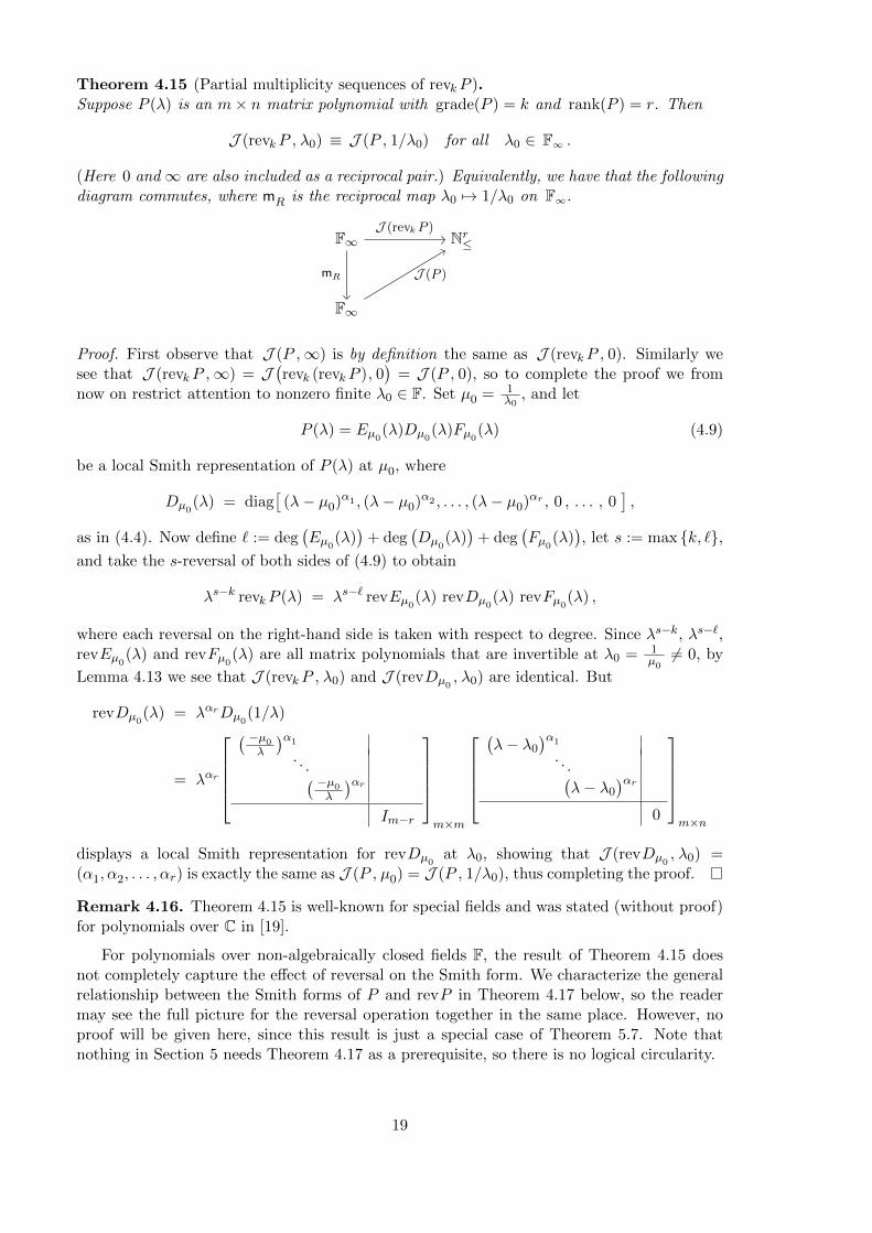
Theorem 4.15 (Partial multiplicity sequences of revkP ).Suppose P (λ) is an m× n matrix polynomial with grade(P ) = k and rank(P ) = r. Then
J (revkP , λ0) ≡ J (P , 1/λ0) for all λ0 ∈ F∞ .
(Here 0 and∞ are also included as a reciprocal pair.) Equivalently, we have that the followingdiagram commutes, where mR is the reciprocal map λ0 7→ 1/λ0 on F∞.
F∞ Nr≤
F∞
J (revkP )
mR J (P )
Proof. First observe that J (P ,∞) is by definition the same as J (revkP , 0). Similarly wesee that J (revkP ,∞) = J
(revk (revkP ), 0
)= J (P , 0), so to complete the proof we from
now on restrict attention to nonzero finite λ0 ∈ F. Set µ0 = 1λ0
, and let
P (λ) = Eµ0(λ)Dµ0(λ)Fµ0(λ) (4.9)
be a local Smith representation of P (λ) at µ0, where
Dµ0(λ) = diag
[(λ− µ0)α1 , (λ− µ0)α2 , . . . , (λ− µ0)αr , 0 , . . . , 0
],
as in (4.4). Now define ` := deg(Eµ0(λ)
)+ deg
(Dµ0
(λ))
+ deg(Fµ0(λ)
), let s := max {k, `},
and take the s-reversal of both sides of (4.9) to obtain
λs−k revkP (λ) = λs−` revEµ0(λ) revDµ0(λ) revFµ0(λ) ,
where each reversal on the right-hand side is taken with respect to degree. Since λs−k, λs−`,revEµ0(λ) and revFµ0(λ) are all matrix polynomials that are invertible at λ0 = 1
µ06= 0, by
Lemma 4.13 we see that J (revkP , λ0) and J (revDµ0, λ0) are identical. But
revDµ0(λ) = λαrDµ0
(1/λ)
= λαr
( −µ0
λ
)α1
. . .( −µ0λ
)αr
Im−r
m×m
(λ− λ0
)α1
. . .(λ− λ0
)αr
0
m×n
displays a local Smith representation for revDµ0at λ0, showing that J (revDµ0
, λ0) =(α1, α2, . . . , αr) is exactly the same as J (P , µ0) = J (P , 1/λ0), thus completing the proof.
Remark 4.16. Theorem 4.15 is well-known for special fields and was stated (without proof)for polynomials over C in [19].
For polynomials over non-algebraically closed fields F, the result of Theorem 4.15 doesnot completely capture the effect of reversal on the Smith form. We characterize the generalrelationship between the Smith forms of P and revP in Theorem 4.17 below, so the readermay see the full picture for the reversal operation together in the same place. However, noproof will be given here, since this result is just a special case of Theorem 5.7. Note thatnothing in Section 5 needs Theorem 4.17 as a prerequisite, so there is no logical circularity.
19
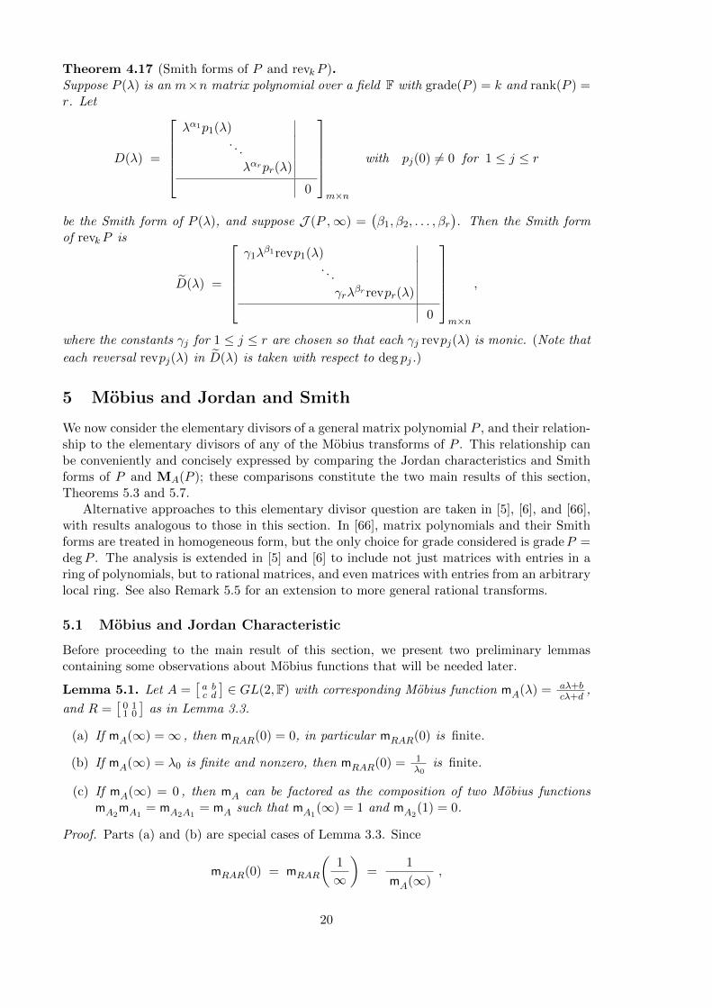
Theorem 4.17 (Smith forms of P and revkP ).Suppose P (λ) is an m×n matrix polynomial over a field F with grade(P ) = k and rank(P ) =r. Let
D(λ) =
λα1p1(λ)
. . .
λαrpr(λ)
0
m×n
with pj(0) 6= 0 for 1 ≤ j ≤ r
be the Smith form of P (λ), and suppose J (P ,∞) =(β1, β2, . . . , βr
). Then the Smith form
of revkP is
D(λ) =
γ1λ
β1revp1(λ). . .
γrλβrrevpr(λ)
0
m×n
,
where the constants γj for 1 ≤ j ≤ r are chosen so that each γj revpj(λ) is monic. (Note that
each reversal revpj(λ) in D(λ) is taken with respect to deg pj.)
5 Mobius and Jordan and Smith
We now consider the elementary divisors of a general matrix polynomial P , and their relation-ship to the elementary divisors of any of the Mobius transforms of P . This relationship canbe conveniently and concisely expressed by comparing the Jordan characteristics and Smithforms of P and MA(P ); these comparisons constitute the two main results of this section,Theorems 5.3 and 5.7.
Alternative approaches to this elementary divisor question are taken in [5], [6], and [66],with results analogous to those in this section. In [66], matrix polynomials and their Smithforms are treated in homogeneous form, but the only choice for grade considered is gradeP =degP . The analysis is extended in [5] and [6] to include not just matrices with entries in aring of polynomials, but to rational matrices, and even matrices with entries from an arbitrarylocal ring. See also Remark 5.5 for an extension to more general rational transforms.
5.1 Mobius and Jordan Characteristic
Before proceeding to the main result of this section, we present two preliminary lemmascontaining some observations about Mobius functions that will be needed later.
Lemma 5.1. Let A =[a bc d
]∈ GL(2,F) with corresponding Mobius function mA(λ) = aλ+b
cλ+d,
and R =[0 11 0
]as in Lemma 3.3.
(a) If mA(∞) =∞ , then mRAR(0) = 0, in particular mRAR(0) is finite.
(b) If mA(∞) = λ0 is finite and nonzero, then mRAR(0) = 1λ0
is finite.
(c) If mA(∞) = 0 , then mA can be factored as the composition of two Mobius functionsmA2
mA1= mA2A1
= mA such that mA1(∞) = 1 and mA2
(1) = 0.
Proof. Parts (a) and (b) are special cases of Lemma 3.3. Since
mRAR(0) = mRAR
(1
∞
)=
1
mA(∞),
20
for part (a) we have mRAR(0) = 1∞ = 0 , and for part (b) we have mRAR(0) = 1
λ0.
For part (c), it suffices to find an appropriate factorization A2A1 for A. First observe thatmA(∞) = 0 implies that A
[10
]=[0c
]for some nonzero c; hence A =
[0 bc d
]with b 6= 0 and
c 6= 0, since A is nonsingular. Then
A2A1 =
[−b bc− d d
] [1 01 1
]=
[0 bc d
]= A
is one such factorization, since A1
[10
]=[11
]implies that mA1
(∞) = 1, and A2
[11
]=[0c
]with c 6= 0 implies that mA2
(1) = 0.
Lemma 5.2. Suppose A =[a bc d
]∈ GL(2,F), with corresponding Mobius function mA(λ) =
aλ+bcλ+d
. If µ0 and mA(µ0) are both finite elements of F∞, then we have the following identity
in the field of rational functions F(µ):
(cµ+ d)[mA(µ)−mA(µ0)
]=
detA
(cµ0 + d)(µ− µ0) .
Proof. Since mA(µ0) is finite, the quantity cµ0+d is nonzero. Thus from the simple calculation
(cµ0 + d)(cµ+ d)[mA(µ)−mA(µ0)
]=
[(aµ+ b)(cµ0 + d)− (aµ0 + b)(cµ+ d)
]=
[(ad− bc)µ− (ad− bc)µ0
]= (detA) (µ− µ0) ,
the result follows immediately.
Theorem 5.3 (Partial multiplicity sequences of Mobius transforms).Let P (λ) be an m×n matrix polynomial over a field F with grade(P ) = k and rank(P ) = r,and let A ∈ GL(2,F) with associated Mobius transformation MA and Mobius function mA.Then for any µ0 ∈ F∞,
J(MA(P ), µ0
)≡ J
(P ,mA(µ0)
). (5.1)
Equivalently, we may instead write
J(MA(P ),mA−1(µ0)
)≡ J
(P , µ0
), (5.2)
or assert that the following diagram commutes.
F∞ Nr≤
F∞
J(MA(P )
)
mA J (P )mA−1
Proof. The proof proceeds in five cases, depending on various combinations of the numbers µ0and λ0 := mA(µ0) being finite, infinite, or nonzero. Throughout the proof we have A =
[a bc d
].
Case 1 [µ0 and λ0 = mA(µ0) are both finite ]: First observe that mA(µ0) being finite meansthat cµ0 + d 6= 0, a fact that will be used implicitly throughout the argument. Now let
P (λ) = Eλ0(λ)Dλ0(λ)Fλ0(λ) (5.3)
be a local Smith representation for P (λ) at λ0, where Dλ0(λ) is as in (4.4); hence by The-orem 4.10 we have (κ1, κ2, . . . , κr) = J (P, λ0) = (α1, α2, . . . , αr) is the partial multiplicity
21
sequence of P at λ0, and degDλ0(λ) = αr. Now define ` := deg(Eλ0(λ)
)+ deg
(Dλ0(λ)
)+
deg(Fλ0(λ)
), and let s := max {k, `}. Then by substituting λ = mA(µ) in (5.3) and pre-
multiplying by (cµ+ d)s we obtain
(cµ+ d)sP(mA(µ)
)= (cµ+ d)sEλ0
(mA(µ)
)Dλ0
(mA(µ)
)Fλ0(mA(µ)
),
or equivalently
(cµ+ d)s−k[MA(P )(µ)
]=[(cµ+ d)s−` MA
(Eλ0
)(µ)]·[(cµ+ d)αrDλ0
(mA(µ)
)]·[MA
(Fλ0)(µ)],
where the Mobius transforms MA
(Eλ0
)and MA
(Fλ0)
are taken with respect to degree ineach case. Since (cµ + d)s−k, (cµ + d)s−`, MA
(Eλ0
)(µ), and MA
(Fλ0)(µ) are all matrix
polynomials that are invertible at µ = µ0, we see by Lemma 4.13 that
J(MA(P ), µ0
)≡ J
((cµ+ d)αrDλ0
(mA(µ)
), µ0
).
We can now simplify (cµ+ d)αrDλ0
(mA(µ)
)even further using Lemma 5.2 and obtain
(cµ+ d)αrDλ0
(mA(µ)
)= (cµ+ d)αr
(mA(µ)− λ0
)α1
. . .(mA(µ)− λ0
)αr
0
m×n
= (cµ+ d)αr
(mA(µ)−mA(µ0)
)α1
. . .(mA(µ)−mA(µ0)
)αr
0
m×n
= G(µ)
(µ− µ0
)α1
. . .(µ− µ0
)αr
0
m×n
, (5.4)
where G(µ) is the diagonal matrix polynomial
G(µ) =
βα1(cµ+ d)αr−α1
βα2(cµ+ d)αr−α2
. . .
βαr(cµ+ d)αr−αr
Im−r
m×m
with β =detA
(cµ0 + d).
Since G(µ) is invertible at µ = µ0, we can now read off from the local Smith representation(5.4) that
J((cµ+ d)αrDλ0
(mA(µ)
), µ0)
= (α1, α2, . . . , αr)
= J (P , λ0) = J (P ,mA(µ0)) ,
and the proof for Case 1 is complete.
22
Case 2 [µ0 and λ0 = mA(µ0) are both ∞ ]:Using the fact that R as in Example 3.7, Definition 4.2, and Lemma 5.1(a) satisfies R2 = I,
we have
J(MA(P ),∞
)= J
(MR
(MA(P )
), 0)
= J(MAR(P ), 0
)= J
(MRAR
(MR(P )
), 0)
= J(MR(P ),mRAR(0)
)= J
(MR(P ), 0
)= J
(P ,∞
)= J (P ,mA(µ0)) .
The first equality is by Definition 4.2, the second and third by Theorem 3.18(b) together withR2 = I, the fourth and fifth by Case 1 together with Lemma 5.1(a), and the last equality byDefinition 4.2.
Case 3 [µ0 =∞, but λ0 = mA(µ0) is finite and nonzero ]:
J(MA(P ),∞
)= J
(MRAR
(MR(P )
), 0)
= J(MR(P ),mRAR(0)
)= J
(MR(P ), 1/λ0
)= J (P , λ0) = J
(P ,mA(µ0)
).
The first equality condenses the first three equalities of Case 2, the second and third are byLemma 5.1(b) together with Case 1, the fourth equality is by Theorem 4.15, and the lastequality just uses the definition of λ0 for this case.
Case 4 [µ0 = ∞ and λ0 = mA(µ0) = 0 ]: This case uses Lemma 5.1(c), which guaranteesthat any mA with the property that mA(∞) = 0 can always be factored as a compositionof Mobius functions mA2
mA1= mA such that mA1
(∞) = 1 and mA2(1) = 0. Using such a
factorization we can now prove Case 4 as a consequence of Case 3 and Case 1.
J(MA(P ), µ0
)= J
(MA2A1
(P ),∞)
= J(MA1
(MA2
(P )),∞)
= J(MA2(P ),mA1
(∞))
= J(MA2(P ), 1
)= J
(P ,mA2
(1))
= J (P , 0) = J(P ,mA(µ0)
).
The first equality invokes the factorization, the second is by Theorem 3.18(b), the thirdequality is by Case 3, the fifth equality is by Case 1, and the last equality uses the definitionof λ0 for this case.
Case 5 [µ0 is finite, and λ0 = mA(µ0) = ∞ ]: For this final case we first need to observethat mA(µ0) =∞ implies that mA−1(∞) = µ0.
J(MA(P ), µ0
)= J
(MA(P ),mA−1(∞)
)= J
(MA−1
(MA(P )
),∞)
= J(P ,∞
)= J
(P ,mA(µ0)
).
The first equality invokes the observation, the second uses Case 3 and 4, the third followsfrom Theorem 3.18(c), and the last equality uses the definition of λ0 for this case.
Theorem 5.3 provides a beautiful and substantial generalization of Theorem 4.15, since thereversal operator revkP is just the particular Mobius transformation induced by the matrixR, as described in Example 3.7.
23
Remark 5.4. It should be noted that the relationship proved in Theorem 5.3 also holds fortruncated Jordan characteristic, i.e.,
J(MA(P ), λ0
)= J
(P ,mA(λ0)
)for every λ0 ∈ F∞ ,
for any matrix polynomial P and any Mobius transformation MA. This follows immediatelyby applying Remark 4.8 to the corresponding result in Theorem 5.3 for the “ordinary” Jordancharacteristic.
Remark 5.5. In view of the results in this section, we suggested that the Jordan characteristicmay behave in a manner analogous to (5.1) under more general rational transforms of matrixpolynomials. This topic has been considered in work by V. Noferini [53].
5.2 Mobius and the Smith Form
The results of Section 5.1 now enable us to find explicit formulas for the Smith form of anyMobius transform of a matrix polynomial P in terms of the Smith form of P itself. To derivethese we will make use of the following lemma.
Lemma 5.6 (Mobius transforms of scalar polynomials).Suppose A =
[a bc d
]∈ GL(2,F), with corresponding Mobius function mA(λ) = aλ+b
cλ+d. Con-
sider any scalar polynomial of the form p(λ) = (λ−λ1)α1(λ−λ2)α2 · · · (λ−λk)αk where λj ∈ Fare distinct finite numbers. Let r = α1 +α2 + · · ·+αk , and define µj to be the unique distinctelements of F∞ so that λj = mA(µj) for j = 1, . . . , k.
(a) If λj 6= mA(∞) for j = 1, . . . , k, then[MA(p)
](µ) = γ(µ− µ1)α1(µ− µ2)α2 · · · (µ− µk)αk ,
where MA is taken with respect to degree, and
γ =(detA)r
(cµ1 + d)α1(cµ2 + d)α2 · · · (cµk + d)αk,
is a finite nonzero constant. (Note that all terms in the denominator of γ are nonzerosince each mA(µj) = λj is finite.)
(b) If λ1 = mA(∞), and so λj 6= mA(∞) for all j = 2, . . . , k, then[MA(p)
](µ) = γ (µ− µ2)α2 · · · (µ− µk)αk ,
where MA is taken with respect to degree, and
γ =(detA)r
(−c)α1(cµ2 + d)α2 · · · (cµk + d)αk,
is a nonzero constant. (Note that all terms in the denominator of γ are nonzero sinceeach mA(µj) = λj is finite. Also mA(∞) = λ1 being finite implies that c 6= 0.)
Observe that in this case deg MA(p) is strictly less than deg p, since the term (λ−λ1)α1
is effectively swallowed up by the Mobius transform MA .
Proof. (a) First consider the case where p(λ) consists of a single linear factor (λ− λj). Thenby the definition of MA and Lemma 5.2 we have
MA(λ− λj) = (cµ+ d)[mA(µ)− λj
]= (cµ+ d)
[mA(µ)−mA(µj)
]=
detA
(cµj + d)(µ− µj).
24
The result of part (a) now follows by applying the multiplicative property of Mobius trans-formations as described in Corollary 3.24(a).
(b) First observe that λ1 being finite with λ1 = mA(∞) means that λ1 = a/c with c 6= 0.Then we have
MA(λ− λ1) = (cµ+ d)[ aµ+ b
cµ+ d− a
c
]= (aµ+ b)− a
c(cµ+ d) = b− ad
c=
detA
−c.
The strategy of part (a) can now be used, mutatis mutandis, to yield the desired result.
Theorem 5.7 (Smith form of Mobius transform).Let P (λ) be an m× n matrix polynomial over a field F with k = grade(P ) and r = rank(P ).Suppose
D(λ) =
λα1p1(λ)
. . .
λαrpr(λ)
0
m×n
with pj(0) 6= 0 for 1 ≤ j ≤ r
is the Smith form of P (λ), and J (P ,∞) = (β1, β2, . . . , βr). Then for A =[a bc d
]∈ GL(2,F)
with associated Mobius function mA(µ) = aµ+bcµ+d
and Mobius transformation MA , the Smith
form of the m× n matrix polynomial MA(P )(µ) is
DA(µ) =
γ1(aµ+ b)α1(cµ+ d)β1MA(p1)(µ)
. . .
γr(aµ+ b)αr(cµ+ d)βrMA(pr)(µ)
0
m×n
, (5.5)
where the constants γj are chosen so that each invariant polynomial di(µ) in DA(µ) is monic.Here each scalar Mobius transform MA(pj) is taken with respect to deg(pj).
Proof. First we show that DA(µ) in (5.5) is a Smith form over the field F for some matrix
polynomial. Since the diagonal entries dj(µ) of DA(µ) are monic polynomials in F[µ] by
definition, we only need to establish the divisibility chain property dj(µ)| dj+1(µ) for j =1, . . . , r−1. Clearly we have α1 ≤ α2 ≤ · · · ≤ αr and β1 ≤ β2 ≤ · · · ≤ βr, since (α1, α2, . . . , αr)and (β1, β2, . . . , βr) are both partial multiplicity sequences for P . Also MA(pj) |MA(pj+1)
follows from pj |pj+1 by Corollary 3.24. Thus dj | dj+1, and hence DA is a Smith form.
It remains to show that DA(µ) is the Smith form of the particular matrix polynomialMA(P ). Recall from Remark 4.6 that a Smith form of a polynomial over a field F is completelydetermined by the finite part of its Jordan characteristic over the algebraic closure F. Thusthe proof will be complete once we show that DA and MA(P ) have the same finite Jordancharacteristic, i.e.,
J(DA , µ0
)= J
(MA(P ), µ0
)(5.6)
for all finite µ0 ∈ F.Since the partial multiplicity sequences of any matrix polynomial are trivial for all but
finitely many µ0, (5.6) will automatically be satisfied for almost all µ0 ∈ F. Our strategy,therefore, is to focus on the sets
SD
:={µ0 ∈ F : J
(DA , µ0
)is nontrivial
}and SM :=
{µ0 ∈ F : J
(MA(P ), µ0
)is nontrivial
},
25
and show that (5.6) holds whenever µ0 ∈ SD ∪ SM. Consequently, SD
= SM and (5.6) holds
for all µ0 ∈ F.
We begin with µ0 ∈ SD. In order to calculate partial multiplicity sequences of DA, first
observe that in each diagonal entry dj(µ) of (5.5), the terms (aµ+b)αj , (cµ+d)βj , and MA(pj)are pairwise relatively prime, and hence share no common roots. Consequently, contributionsto any particular nontrivial partial multiplicity sequence for DA can come either
• from just the (aµ+ b)αj -terms,
• from just the (cµ+ d)βj -terms,
• or from just the MA(pj)-terms.
That (aµ + b) is relatively prime to (cµ + d) follows from the nonsingularity of A. If either(aµ+ b) or (cµ+ d) were a factor of MA(pj), then by Lemma 5.6, pj(λ) would have to haveeither mA(−ba ) or mA(−dc ) as a root; however, neither of these is possible, since mA(−ba ) = 0
and mA(−dc ) =∞.
Now consider the possible values of µ0 ∈ SD . Clearly µ0 = −ba is one such possibility, but
only if a 6= 0 and if (α1, α2, . . . , αr) is nontrivial; otherwise all the terms (aµ+b)αj are nonzeroconstants, and are effectively absorbed by the normalizing constants γj . So if µ0 = −b
a ∈ SD,then we have
J(DA ,
−ba
)= (α1, . . . , αr) = J
(D, 0
)= J
(P , 0
)= J
(MA(P ),m−1A (0)
)= J
(MA(P ), −ba
),
and (5.6) holds for µ0 = −ba . Note that the fourth equality is an instance of Theorem 5.3,
which we will continue to use freely throughout the remainder of this argument. Anotherpossible µ0-value in S
Dis µ0 = −d
c , but again only if c 6= 0 and if (β1, β2, . . . , βr) is nontrivial;otherwise all (cµ + d)βj -terms are nonzero constants that get absorbed by the constants γj .If µ0 = −d
c ∈ SD, then we have
J(DA ,
−dc
)= (β1, . . . , βr) = J
(P ,∞
)= J
(MA(P ),m−1A (∞)
)= J
(MA(P ), −dc
),
and (5.6) holds for µ0 = −dc . The only other µ0-values in S
Dare the roots of the polynomial
MA(pr), so suppose µ0 is one of those roots. Then by Lemma 5.6 we have J(DA , µ0
)=
J(D,mA(µ0)
)with a finite mA(µ0), and thus
J(DA , µ0
)= J
(D,mA(µ0)
)= J
(P ,mA(µ0)
)= J
(MA(P ), µ0
),
completing the proof that (5.6) holds for all µ0 ∈ SD.Finally we turn to the µ0-values in SM. By Theorem 5.3 we certainly have
J(MA(P ), µ0
)= J
(P ,mA(µ0)
)for any µ0 ∈ SM. The remainder of the argument depends on whether mA(µ0) is finite orinfinite.
(1) If mA(µ0) is finite, then J(MA(P ), µ0
)= J
(P ,mA(µ0)
)= J
(D,mA(µ0)
), since D is
the Smith form of P . This partial multiplicity sequence is nontrivial since µ0 ∈ SM, soeither mA(µ0) = 0, or λ0 = mA(µ0) 6= 0 is a root of pr(λ). If mA(µ0) = 0, then sinceµ0 is finite we must have a 6= 0 and µ0 = −b
a , and hence J(D,mA(µ0)
)= J
(D, 0
)=
(α1, α2, . . . , αr) = J(DA ,
−ba
)= J
(DA , µ0
), so (5.6) holds. If on the other hand
λ0 = mA(µ0) 6= 0, then since λ0 = mA(µ0) is a root of pr(λ), we have by Lemma 5.6
that J(D,mA(µ0)
)= J
(DA , µ0
), and so once again (5.6) holds.
26
(2) If mA(µ0) =∞, then because µ0 is finite we must have c 6= 0 and µ0 = −dc . In this case
J(MA(P ), µ0
)= J
(P ,∞
)= (β1, β2, . . . , βr) by our choice of notation; this sequence
is nontrivial since µ0 ∈ SM. But (β1, β2, . . . , βr) is equal to J(DA ,
−dc
)when c 6= 0, by
our definition of DA, and so (5.6) holds for this final case.
Thus (5.6) holds for all µ0 ∈ SM, and the proof is complete.
Using the fact that the reversal operator can be viewed as a Mobius transformation, an im-mediate corollary of Theorem 5.7 is the complete characterization of the relationship betweenthe Smith forms of P and revkP , as described earlier (without proof) in Theorem 4.17.
6 Mobius and Invariant Pairs
It is common knowledge, see e.g., [13, 50] for the case of Hamiltonian and symplectic matricesand pencils, that invariant subspaces of matrices and deflating subspaces of matrix pencilsremain invariant under Cayley transformations. In this section, we investigate the analogousquestion for regular matrix polynomials under general Mobius transformations, using theconcept of invariant pair. Introduced in [10] and further developed in [9], this notion extendsthe well-known concepts of standard pair [30] and null pair [8]. Just as invariant subspacesfor matrices or deflating subspaces for pencils can be seen as a generalization of eigenvectors,we can think of invariant pairs of matrix polynomials as a generalization of eigenpairs (x, λ0),consisting of an eigenvector x together with its associated eigenvalue λ0. The concept ofinvariant pair can be a more flexible and useful tool for computation in the context of matrixpolynomials than either eigenpair, null pair, or standard pair [9].
Definition 6.1 (Invariant pair).Let P (λ) =
∑kj=0 λ
jBj be a regular n×n matrix polynomial of grade k over a field F, and let
(X,S) ∈ Fn×m× Fm×m. Then (X,S) is said to be an invariant pair for P (λ) if the followingtwo conditions hold:
(a) P (X,S) :=∑k
j=0BjXSj = 0 , and
(b) Vk(X,S) :=
XXS...
XSk−1
has full column rank.
Example 6.2. The following provides a variety of examples of invariant pairs:
(a) The simplest example of an invariant pair is an eigenpair: with m = 1, a vector-scalarpair (x, λ0) with nonzero x ∈ Fn and λ0 ∈ F is an invariant pair for P if and only if(x, λ0) is an eigenpair for P .
(b) Standard pairs in the sense of [30] are the same as invariant pairs of monic matrixpolynomials over F = C with k = degP and m = nk.
(c) If F = C and S is a single Jordan block associated with the eigenvalue λ0, then thecolumns of the matrix X in any invariant pair (X,S) form a Jordan chain for P (λ)associated with the eigenvalue λ0 . It is worth noting that Jordan chains constitutean alternative to the Smith form as a means of defining the Jordan characteristic of amatrix polynomial at an eigenvalue λ0 ∈ F. See [30] for more on Jordan chains.
27
(d) If F = C, then a right null pair for P (in the sense of [8]) associated with λ0 ∈ C is thesame as an invariant pair (X,S), where the spectrum of S is just {λ0} and the size mcoincides with the algebraic multiplicity of λ0 as an eigenvalue of P .
(e) For regular pencils, invariant pairs are closely related to the notion of deflating subspace.
Recall that for an n×n pencil L(λ) = λA+B, an m-dimensional subspace X ⊆ Fn is adeflating subspace for L(λ), see e.g., [11, 39, 60], if there exists another m-dimensionalsubspace Y ∈ Fn such that AX ⊆ Y and BX ⊆ Y. Letting the columns of X,Y ∈ Fn×mform bases for X and Y, respectively, it follows that these containment relations can beequivalently expressed as AX = YWA and BX = YWB, for some matrices WA,WB ∈Fm×m.
Now if AX = Y, i.e., if X ∩kerA = {0}, then WA is invertible, so that Y = AXW−1A andBX = AXW−1A WB. Letting S := −W−1A WB, we see that L(X,S) = AXS + BX = 0,and hence (X,S) is an invariant pair for L(λ). Similarly if X ∩ kerB = {0}, thenWB is invertible, and (X, S) with S := −W−1B WA is an invariant pair for the pencil
revL(λ) = λB + A. Later (in Definition 6.7) we will refer to such a pair (X, S) as areverse invariant pair for L(λ).
Conversely, if (X,S) is an invariant pair for L(λ), then X , the subspace spanned by thecolumns of X, will be a deflating subspace for L(λ). To see why this is so, first observethat L(X,S) = AXS +BX = 0 implies that BX ⊆ AX . Thus if dimX = m, then anym-dimensional subspace Y ∈ Fn such that AX ⊆ Y will witness that X is a deflatingsubspace for L.
Remark 6.3. Definition 6.1 follows the terminology in [10], where both conditions (a) and(b) are required for a pair (X,S) to be an invariant pair for P . A weaker notion is introducedin [9], where condition (a) alone suffices for (X,S) to be called an invariant pair; if conditions(a) and (b) are both met, then (X,S) is called a minimal invariant pair. This weaker notionof invariant pair has several drawbacks that significantly detract from its usefulness. First,weak invariant pairs may contain redundant information, and even be arbitrarily large; forexample, if (x, λ0) is any eigenpair for P , then X = [x x . . . x ]n×m with S = λ0Im givesweak invariant pairs for P of unbounded size. The full column rank condition (b), though,forces m ≤ kn since Vk(X,S) has only kn rows. A more significant drawback of weakinvariant pairs (X,S) concerns the spectrum σ(S) and its relationship to σ(P ). The intendedpurpose of S is to capture some portion of the eigenvalues of P (λ), i.e., σ(S) ⊆ σ(P ), whileeigenvector information corresponding to this subset σ(S) is captured in X. We will see inProposition 6.6 that any invariant pair in the sense of Definition 6.1 does indeed have thedesired containment property σ(S) ⊆ σ(P ). However, a weak invariant pair may includemany spurious eigenvalues, that is, eigenvalues of S that are not in σ(P ). In particular,a weak invariant pair (X,S) with nonzero X and m × m matrix S may have up to m − 1spurious eigenvalues; in general S and P (λ) can only be guaranteed to have one eigenvaluein common. For these reasons we have reserved the more concise term invariant pair for themore important notion, as specified in Definition 6.1.
For polynomials of the special form P (λ) = λIn − B0, the condition in Definition 6.1(a)reduces to P (X,S) = XS − B0X = 0, equivalently to B0X = XS, which is satisfied ifand only if the columns of X span an invariant subspace X of the matrix B0. In this case,condition (b) just means that the columns of X are linearly independent, and thus form abasis for X . The eigenvalues of S are then the eigenvalues of B0 associated with the subspaceX . Certainly an invariant subspace is independent of the choice of basis, and so can also berepresented by the columns of any matrix XT , where T is an invertible m×m transformationmatrix. This observation motivates the following definition.
28
Definition 6.4 (Similarity of pairs).Two pairs (X,S), (X, S) ∈ Fn×m×Fm×m, where F is an arbitrary field, are said to be similarif there exists a nonsingular matrix T ∈ Fm×m such that X = XT and S = T−1ST .
The following basic property of similar pairs is straightforward to prove from the definitions.
Lemma 6.5. If the pairs (X,S) and (X, S) are similar, then one is an invariant pair for aregular matrix polynomial P (λ) if and only if the other one is, too.
This simple observation has an important consequence: if (X,S) is an invariant pair forP (λ), then every eigenvalue of the matrix S is also an eigenvalue of the matrix polynomialP (λ), i.e., S has no spurious eigenvalues as discussed in Remark 6.3. More generally, anyinvariant subspace for S induces an invariant pair for P (λ) that is in a certain sense “con-tained” in (X,S); this is made precise in the following proposition. Here for a matrix Y , weuse Col(Y ) to denote the space spanned by the columns of Y .
Proposition 6.6. Let (X,S) ∈ Fn×m × Fm×m be an invariant pair for the regular matrixpolynomial P (λ) =
∑kj=0 λ
jBj.
(a) Suppose that U ⊆ Fm is an `-dimensional invariant subspace for the matrix S, andT =
[T1 T2
]∈ Fm×m is any nonsingular matrix such that the columns of T1 form a
basis for U , so that
S := T−1ST =
[S11 S120 S22
], where S11 ∈ F`×`.
Then (XT1, S11) is an invariant pair for P (λ) that is “contained” in (X,S) in the sensethat
Col(XT1) ⊆ Col(X) and σ(S11) ⊆ σ(S) .
(b) σ(S) ⊆ σ(P ).
Proof. (a) First observe that (XT, S) is an invariant pair for P (λ), since it is similar to the
invariant pair (X,S). But Sj =
[Sj11 ∗0 ∗
]for all j ≥ 0, so we have
XTSj = X[T1 T2
] [ Sj11 ∗0 ∗
]=[XT1S
j11 ∗
](6.1)
for all j ≥ 0. Hence
0 = P (XT, S) =
k∑j=0
BjXTSj =
k∑j=0
[Bj(XT1)S
j11 ∗
]=[P (XT1, S11) ∗
],
and so P (XT1, S11) = 0, i.e., the pair (XT1, S11) satisfies condition (a) of Definition 6.1.The containments Col(XT1) ⊆ Col(X) and σ(S11) ⊆ σ(S) are immediate; all that remainsis to see why the full column rank condition holds for (XT1, S11). From (6.1) we see thatVk(XT, S) =
[Vk(XT1, S11) ∗
], so the full column rank of Vk(XT1, S11) follows from the
full column rank of Vk(XT, S).
(b) Suppose that λ0 ∈ σ(S), with corresponding eigenvector y ∈ Fm. Then by part (a) with` = 1 we know that (Xy, λ0) is an invariant pair for P . Thus (Xy, λ0) is an eigenpair for Pby Example 6.2, and so λ0 ∈ σ(P ).
29
This proposition shows that invariant pairs enable us to focus on any specific part ofthe finite spectrum of P (λ). Unfortunately, though, invariant pairs can never contain anyinformation about eigenvalues at ∞. To address this deficiency, we introduce the followingconcept, which builds on the correspondence between the eigenvalue ∞ for P (λ) and theeigenvalue zero for revP (λ).
Definition 6.7 (Reverse invariant pairs).Let P (λ) =
∑kj=0 λ
jBj be a regular n × n matrix polynomial with grade k over a field F.
Then a pair (X,S) ∈ Fn×m × Fm×m is called a reverse invariant pair for P (λ) if (X,S) isan invariant pair for revkP (λ), i.e., if
revkP (X,S) :=
k∑j=0
Bk−jXSj = 0 ,
and Vk(X,S) as in Definition 6.1(b) has full column rank.
The next example and proposition provide two simple sources of reverse invariant pairs.
Example 6.8. A nonzero vector x ∈ Fn is an eigenvector associated with the eigenvalue ∞of P (λ) if and only if (x, 0) is a reverse invariant pair for P (λ).
Recall from Theorem 4.15 that reversal has a simple effect on nonzero eigenvalues and theirJordan characteristics, i.e., J (P , λ0) ≡ J (revkP , 1/λ0) for any nonzero λ0. This suggeststhe following connection between invariant pairs and reverse invariant pairs for P .
Proposition 6.9. Suppose P (λ) =∑k
j=0 λjBj is a regular n × n matrix polynomial with
grade k over a field F, and let (X,S) ∈ Fn×m × Fm×m be a matrix pair with nonsingular S.Then (X,S) is an invariant pair for P if and only if (X,S−1) is a reverse invariant pair forP .
Proof. First observe that
P (X,S) · S−k =
k∑j=0
BjXSj−k =
k∑j=0
Bk−jXS−j = revkP (X,S−1)
and
Vk(X,S) · S−(k−1) = (Rk ⊗ In) · Vk(X,S−1) , where Rk :=
[1
. ..
1
]k×k
is the k × k reverse identity. From these relations it is clear that P (X,S) = 0 if and only ifrevkP (X,S−1) = 0, and that Vk(X,S) has full column rank if and only if Vk(X,S−1) does,too. The desired conclusion now follows.
We are now in a position to address the main issue of this section — how Mobius trans-formations interact with invariant pairs. In particular, given an invariant pair (X,S) for P ,is there a naturally corresponding invariant pair for the Mobius transform MA(P )? FromTheorem 5.3 we know that an eigenvalue µ0 of P corresponds to an eigenvalue mA−1(µ0)of MA(P ). But Proposition 6.6 shows that σ(S) ⊆ σ(P ) for any invariant pair (X,S),and hence mA−1
(σ(S)
)⊆ σ
(MA(P )
). Now as long as the matrix mA−1(S) is defined, then
σ(mA−1(S)
)= mA−1
(σ(S)
), and hence σ
(mA−1(S)
)⊆ σ
(MA(P )
). Thus it is reasonable to
conjecture that an invariant pair (X,S) for P will induce an invariant pair (X,mA−1(S)) forthe Mobius transform MA(P ), whenever the matrix mA−1(S) is defined. This conjecture,along with several related variations, is proved in Theorem 6.11. We begin with the followinglemma, whose straightforward proof is only sketched.
30
Lemma 6.10. Suppose φj(λ) ∈ F[λ] for j = 0, . . . , k are arbitrary scalar polynomials over
F, and P (λ) =∑k
j=0 φj(λ)Bj is any n× n matrix polynomial expressed in terms of the φj’s.
If (X,S) ∈ Fn×m × Fm×m is any matrix pair, then P (X,S) =∑k
j=0BjXφj(S).
Proof. First show that the additive property (P+Q)(X,S) = P (X,S)+Q(X,S) holds for anypolynomials P and Q of the same size, by expressing P and Q in the standard basis and thenusing the defining formula given in Definition 6.1(a). Then show that P (X,S) = BXφ(S)for any polynomial of the special form P (λ) = φ(λ)B. Combining the additive property withthe special case gives the desired result.
Theorem 6.11 (Invariant pairs of Mobius transforms).Let P (λ) =
∑kj=0 λ
jBj be an n × n matrix polynomial over a field F and let (X,S) be a
matrix pair in Fn×m × Fm×m. Furthermore, let
A =
[a bc d
]∈ GL(2,F) , mA(λ) =
aλ+ b
cλ+ d, and R =
[0 11 0
].
(a) Suppose that either c = 0, or c 6= 0 and ac 6∈ σ(S). Then
(X,S) is an invariant pair for P ⇐⇒ (X,mA−1(S)) is an invariant pair for MA(P ).
(b) Suppose that either d = 0, or d 6= 0 and bd 6∈ σ(S). Then
(X,S) is an invariant pair for P ⇐⇒ (X,m(AR)−1(S)) is a reverse invariant pair for
MA(P ).
(c) Suppose that either a = 0, or a 6= 0 and ca 6∈ σ(S). Then
(X,S) is a reverse invariant pair for P ⇐⇒ (X,m(RA)−1(S)) is an invariant pair for
MA(P ).
(d) Suppose that either b = 0, or b 6= 0 and db 6∈ σ(S). Then
(X,S) is a reverse invariant pair for P ⇐⇒ (X,m(RAR)−1(S)) is a reverse invariant
pair for MA(P ).
Proof. (a) The given hypothesis on A and S (i.e., either that c = 0 (and hence a, d 6= 0), orthat c 6= 0 with a
c not an eigenvalue of S) is exactly the condition needed to guarantee that
the matrix (−cS + aI) is nonsingular, and thus that S := mA−1(S) = (dS − bI)(−cS + aI)−1
introduced in (3.8) is well defined. Now mA( −dc ) =∞, so the invertibility of Mobius functions
implies that mA−1(∞) = −dc . But ∞ is not an eigenvalue of the matrix S, so −d
c is not
an eigenvalue of mA−1(S) = S; thus under these conditions the matrix (cS + dI) is also
nonsingular, no matter whether c is zero or nonzero. Consequently, mA(S) = (aS + bI)(cS +dI)−1 is well defined and equal to S.
To show the equivalence of (X,S) and (X, S) being invariant pairs, we consider the twodefining conditions in turn. A direct calculation using Lemma 6.10 first establishes a generalrelationship between MA(P )(X, S) and P (X,S):
MA(P )(X, S) =
k∑j=0
BjX(aS + bI)j(cS + dI)k−j
=
k∑j=0
BjX((aS + bI)(cS + dI)−1
)j · (cS + dI)k
= P(X,mA(S)
)· (cS + dI)k
= P (X,S) · (cS + dI)k .
31
Then the nonsingularity of (cS+dI) implies that MA(P )(X, S) = 0 if and only if P (X,S) = 0,so Definition 6.1(a) is satisfied either for both pairs or for neither of them.
For condition (b) in Definition 6.1, we first see how Vk(X,S) and Vk(X, S) are related.Since S = mA(S), we have
Vk(X,S) · (cS + dI)k−1 =
X
XmA(S)...
XmA(S)k−1
(cS + dI)k−1 =
Xq1(S)
Xq2(S)...
Xqk(S)
, (6.2)
where each qi is a scalar polynomial of degree at most k − 1. Assembling all the coefficientsof the qi polynomials (row-wise) into a k × k matrix Q, we see that the last matrix in (6.2)can be expressed as (Q ⊗ In)Vk(X, S), and so
(Q ⊗ In) · Vk(X, S) = Vk(X,S) · (cS + dI)k−1 (6.3)
gives a general relationship between Vk(X, S) and Vk(X,S). The nonsingularity of (cS + dI)now implies that
rankVk(X, S) ≥ rankVk(X,S) .
Interchanging the roles of S and S, and using that S = mA−1(S), a similar argument showsthat
(Q⊗ In) · Vk(X,S) = Vk(X, S) · (−cS + aI)k−1
for some k × k matrix of coefficients Q. Then the nonsingularity of (−cS + aI) implies that
rankVk(X, S) ≤ rankVk(X,S) ,
and thus rankVk(X, S) = rankVk(X,S). Consequently Definition 6.1(b) is satisfied eitherfor both or for neither of the two pairs. This completes the proof of part (a).
(b) Consider the Mobius transformation induced by the matrix B = AR =[b ad c
]. Then the
given hypothesis on d and b allows us to use part (a) to conclude that
(X,S) is an invariant pair for P ⇐⇒ (X,mB−1(S)) is an invariant pair for MB(P ).
But an invariant pair for MB(P ) = MAR(P ) = MR
(MA(P )
)= revkMA(P ) is a reverse
invariant pair for MA(P ), so the result is proved.
(c) By definition, (X,S) is a reverse invariant pair for P if and only if (X,S) is an invariantpair for revkP . Applying (a) to the polynomial revkP , with Mobius transformation inducedby the matrix RA =
[c da b
], we obtain that (X,S) is an invariant pair for revkP if and only
if (X,m(RA)−1(S)) is an invariant pair for MRA(revkP ) = MA
(MR(revkP )
)= MA(P ), and
the result is proved.
(d) The argument is analogous to that for (c). Apply (a) to the polynomial revkP , usingthe Mobius transformation induced by the matrix RAR =
[d cb a
]. Then we obtain that
(X,S) is an invariant pair for revkP if and only if (X,m(RAR)−1(S)) is an invariant pair for
MRAR(revkP ) = MR
(MA
(MR(revkP )
))= revkMA(P ).
Remark 6.12. From Theorem 6.11, it is straightforward to show that if (x, λ0) is anyeigenpair of the regular matrix polynomial P , including any eigenpair with λ0 = ∞, then(x,mA−1(λ0)) will always be an eigenpair of MA(P ). Thus we see that eigenvectors of matrixpolynomials are preserved by any Mobius transformation. Are Jordan chains also preservedby Mobius transformations? Approaching this question via the usual definition of Jordanchains [30] leads to technical difficulties; the invariant pair point of view, though, provides a
32
clearer view of the situation. Recall from Example 6.2(c) that if (X,S) is an invariant pairfor P (λ) and S = Jm(λ0) is the m×m Jordan block associated with the eigenvalue λ0, thenthe columns of X form a Jordan chain for P (λ) associated with the eigenvalue λ0. Now byTheorem 6.11 we know that (X,mA−1(S)) is the corresponding invariant pair for MA(P ), aslong as mA−1(S) is defined. But the matrix mA−1(S) will in general not be in Jordan form,although it will always be upper triangular and Toeplitz, with mA−1(λ0) on the diagonal.Consequently the columns of X will usually not form a Jordan chain for MA(P ) associatedwith the eigenvalue mA−1(λ0). One notable exception is when m = 2; in this case the 2 × 2matrix mA−1(S) is always close enough to Jordan form that a simple scaling suffices to recovera Jordan chain of length two for MA(P ) from the two columns of X. In summary, then, wesee that Jordan chains are not in general preserved under Mobius transformations. Thus it isreasonable to expect that invariant pairs will usually be a more natural and convenient toolthan Jordan chains in situations where Mobius transformations are involved.
An intrinsic limitation of any invariant pair of a matrix polynomial P is that it can onlycontain information about the finite spectrum of P , since that spectral information is recordedin a matrix S. A reverse invariant pair for P overcomes this limitation, but at the cost ofnot being able to contain information about the eigenvalue 0. These limitations make itclear, for example, why the notion of a deflating subspace of a regular pencil, as described inExample 6.2(e), is (for pencils) more general than either invariant pair or reverse invariantpair; deflating subspaces have no trouble in simultaneously accommodating both zero andinfinite eigenvalues.
The “forbidden eigenvalue” phenomenon of Theorem 6.11 is another setting in which theseintrinsic limitations of (reverse) invariant pairs manifest themselves. For example, suppose wehave an invariant pair (X,S) for a matrix polynomial P , and we wish to find an invariant pairwith the same first component X for a Mobius transform MA(P ). Since such an invariantpair for MA(P ) would have to include all of mA−1
(σ(S)
)among its associated eigenvalues,
we must make sure that mA−1
(σ(S)
)does not contain ∞, equivalently that mA(∞) 6∈ σ(S).
This mA(∞) is the “forbidden eigenvalue” ac of Theorem 6.11(a). Analogous considerations
account for the “forbidden eigenvalues” in each of the other parts of Theorem 6.11.Suppose now that we have an invariant pair (X,S) for P , where S contains both of the
forbidden eigenvalues in parts (a) and (b) of Theorem 6.11. Then it seems that nothing canbe said about the effect of the Mobius transformation MA on the invariant pair; Theorem 6.11cannot be used to find either an invariant or a reverse invariant pair for MA(P ) with firstcomponent X. However, if we can “separate” the two forbidden eigenvalues from each other,then it is possible to say something useful about the effect of MA on the invariant pair(X,S). This procedure is illustrated in the following remark. An analogous procedure can beformulated if we start instead with a reverse invariant pair for P .
Remark 6.13. Let P (λ) =∑k
j=0 λjBj be a regular n× n matrix polynomial over a field F,
and let
A =
[a bc d
]∈ GL(2,F) and mA(λ) =
aλ+ b
cλ+ d, with a, c, d 6= 0 .
Suppose (X,S) ∈ Fn×m×Fm×m is an invariant pair for P with ac ,
bd ∈ σ(S), so that the spec-
trum of S contains the two “forbidden” eigenvalues from Theorem 6.11(a) and (b). Observethat a
c = mA(∞) and bd = mA(0) must be distinct elements of F, since mA is a bijection on
F∞. Now there exists a nonsingular matrix T ∈ Fm×m such that
X := XT =[X1 X2
]and S := T−1ST =
[S1 00 S2
],
where X1 ∈ Fn×`, X2 ∈ Fn×(m−`), S1 ∈ F`×`, S2 ∈ F(m−`)×(m−`) for some 1 ≤ ` < m,and where a
c 6∈ σ(S1) and 0, bd 6∈ σ(S2). Thus the eigenvalues bd and a
c are separated into
33
distinct blocks S1 and S2, respectively, where S2 can even be chosen to be invertible. (Onepossible way to do this separation is to bring S into rational canonical form [37, Sect. 3.4]over the field F, with one Frobenius companion block for each F-elementary divisor of S; thengather all companion blocks associated with eigenvalues 0 and b
d in S1, all companion blocksassociated with a
c in S2, and distribute all other companion blocks arbitrarily among S1 and
S2.) Then (X, S) is an invariant pair for P by Lemma 6.5, and (X1, S1) and (X2, S2) areinvariant pairs for P by Proposition 6.6. Furthermore, Theorem 6.11 can now be applied to(X1, S1) and (X2, S2) individually to conclude that (X1,mA−1(S1)) is an invariant pair forMA(P ) and (X2,m(AR)−1(S2)) is a reverse invariant pair for MA(P ).
An alternative approach to this situation is to organize the data X1, X2, S1, S2 from theprevious paragraph in a slightly different way. We still view (X1, S1) as an invariant pairfor P , but now note that (X2, S
−12 ) is a reverse invariant pair for P , by the discussion in
Example 6.8(b). Then consider the pair (X, S), where
X := X =[X1 X2
]and S :=
[S1 0
0 S−12
];
clearly (X, S) will in general be neither an invariant pair nor a reverse invariant pair for P .However, the matrix
Wk
((X1, S1), (X2, S
−12 ))
:=
X1 X2
(S−12
)k−1X1S1 X2
(S−12
)k−2...
...
X1Sk−11 X2
= Vk(X, S) ·
[I` 0
0(S−12
)k−1]
(6.4)has full column rank, since (X, S) being an invariant pair implies that Vk(X, S) has fullcolumn rank. Thus the pair (X, S) can be viewed as a natural generalization of the notionof a decomposable pair for P , as introduced in [30]. Such a “generalized decomposable pair”consists of an invariant pair together with a reverse invariant pair, satisfying a full rankcondition for a matrix Wk as in (6.4).
Now since ac 6∈ σ(S1) and d
b 6∈ σ(S−12 ), we can apply Theorem 6.11 to the individual pairs(X1, S1) and (X2, S
−12 ) to conclude that (X1,mA−1(S1)) is an invariant pair for MA(P ) and
(X2,m(RAR)−1(S−12 )) is a reverse invariant pair for MA(P ). Then with
M :=
[mA−1(S1) 0
0 m(RAR)−1(S−12 )
],
we claim that (X, M) is a “generalized decomposable pair” for MA(P ) in the same senseas (X, S) is a generalized decomposable pair for P . Letting S1 := mA−1(S1) and S2 :=
m(RAR)−1(S−12 ), all that remains is to see why the matrix
Wk
((X1, S1), (X2, S2)
)=
X1 X2m(RAR)−1(S−12 )k−1
X1mA−1(S1) X2m(RAR)−1(S−12 )k−2
......
X1mA−1(S1)k−1 X2
(6.5)
has full column rank. To do this we employ a strategy analogous to the one used in the proofof Theorem 6.11.
First observe that mA( −dc ) =∞, and hence mA−1(∞) = −dc . But ∞ is not an eigenvalue
of the matrix S1, so −dc is not an eigenvalue of mA−1(S1) = S1, and therefore the matrix
34
(cS1 + dI) is nonsingular. Thus mA(S1) = (aS1 + bI)(cS1 + dI)−1 is well defined and equal to
S1. A similar argument shows that the matrix (bS2 + aI) is also nonsingular, and hence thatmRAR(S2) = (dS2 + cI)(bS2 + aI)−1 = S−12 . Now we use these facts to develop a relationship
between the matrices Wk
((X1, S1), (X2, S
−12 ))
and Wk
((X1, S1), (X2, S2)
).
Wk
((X1, S1), (X2, S
−12 ))·[
(cS1 + dI)k−1 0
0 (bS2 + aI)k−1
]
= Wk
((X1,mA(S1)), (X2,mRAR(S2))
)·[
(cS1 + dI)k−1 0
0 (bS2 + aI)k−1
]
=
X1 (cS1 + dI)k−1 X2 (dS2 + cI)k−1
X1 (cS1 + dI)k−2(aS1 + bI) X2 (dS2 + cI)k−2(bS2 + aI)
X1 (cS1 + dI)k−3(aS1 + bI)2 X2 (dS2 + cI)k−3(bS2 + aI)2...
...
X1 (aS1 + bI)k−1 X2 (bS2 + aI)k−1
=
X1 q1(S1) X2 (revk−1 q1)(S2)
X1 q2(S1) X2 (revk−1 q2)(S2)...
...
X1 qk(S1) X2 (revk−1 qk)(S2)
,where each qi is a scalar polynomial of grade k − 1. Assembling the coefficients of all the qipolynomials row-wise into a k × k matrix Q, then the last matrix can be expressed as
(Q ⊗ In) ·
X1 X2 S
k−12
X1 S1 X2 Sk−22
......
X1 Sk−11 X2
= (Q ⊗ In) · Wk
((X1, S1), (X2, S2)
).
Letting B be the invertible block-diagonal matrix B = diag((cS1 + dI)k−1, (bS2 + aI)k−1
),
we have thus shown that
(Q ⊗ In) · Wk
((X1, S1), (X2, S2)
)= Wk
((X1, S1), (X2, S
−12 ))·B . (6.6)
Observe that the relationship in (6.6) is the analog of that developed in (6.3) for the proof ofTheorem 6.11. From (6.6) it is now immediate that
rankWk
((X1, S1), (X2, S2)
)≥ rankWk
((X1, S1), (X2, S
−12 )),
and hence that Wk
((X1, S1), (X2, S2)
)has full column rank, as desired. Finally, although we
did not need this fact here, it is worth noting that the ranks can be shown to always be equal,by an argument analogous to the one used in the proof of Theorem 6.11.
7 Mobius and Minimal Indices
An important aspect of the structure of a singular matrix polynomial is captured by itsminimal indices and bases. This section investigates the relationship between these quantitiesfor a singular polynomial P and any of its Mobius transforms MA(P ). For the convenienceof the reader, we begin by recalling the definition and basic properties of minimal indices andbases, and then proceed in Section 7.2 to establish the main results.
35
7.1 Minimal Indices and Bases – Definition and Basic Properties
Let F(λ) denote the field of rational functions over F, and F(λ)n the vector space of all n-vectors with entries in F(λ). In this section, elements of F(λ)n will be denoted by notationlike ~x(λ), in order to maintain a clear visual distinction between vectors in F(λ)n and scalarsin F(λ).
An m × n singular matrix polynomial P (λ) has nontrivial right and/or left null vectors,that is, vectors ~x(λ) ∈ F(λ)n and ~y(λ) ∈ F(λ)m such that P (λ)~x(λ) ≡ 0 and ~y(λ)TP (λ) ≡ 0,where ~y(λ)T denotes the transpose of ~y(λ). This leads to the following definition.
Definition 7.1. The right and left nullspaces of the m×n matrix polynomial P (λ), denotedrespectively by Nr(P ) and N`(P ), are the subspaces
Nr(P ) :={~x(λ) ∈ F(λ)n : P (λ)~x(λ) ≡ ~0
},
N`(P ) :={~y(λ) ∈ F(λ)m : ~y(λ)TP (λ) ≡ ~0T
},
respectively.
A vector polynomial is a vector all of whose entries are polynomials in the variable λ.For any subspace of F(λ)n, it is always possible to find a basis consisting entirely of vectorpolynomials; simply take an arbitrary basis and multiply each vector by the denominators ofits entries. The degree of a vector polynomial is the largest degree of its components, and theorder of a polynomial basis is defined as the sum of the degrees of its vectors [25, p. 494].Then we have the following definition of a minimal basis for a rational subspace.
Definition 7.2. Let S be a subspace of F(λ)n. The order of S, denoted ord(S), is theleast order among all vector polynomial bases of S, and a minimal basis of S is any vectorpolynomial basis of S that attains this least order.
In [25] it is shown that for any given subspace S of F(λ)n, the ordered list of degrees of thevector polynomials in any minimal basis of S is always the same; these degrees are the minimalindices of S. Specializing S to be the left and right nullspaces of a singular matrix polynomialgives Definition 7.3; here the degree of a vector polynomial ~p(λ) is denoted deg ~p(λ).
Definition 7.3 (Minimal indices and bases of a singular matrix polynomial).For a singular matrix polynomial P (λ), let the sets
{~y1(λ), . . . , ~yq(λ)
}and
{~x1(λ), . . . , ~xp(λ)
}be minimal bases, respectively, of the left and right nullspaces of P (λ), ordered such thatdeg(~y1) ≤ deg(~y2) ≤ · · · ≤ deg(~yq) and deg(~x1) ≤ · · · ≤ deg(~xp). Let ηi = deg(~yi) fori = 1, . . . , q and εj = deg(~xj) for j = 1, . . . , p. Then η1 ≤ η2 ≤ · · · ≤ ηq and ε1 ≤ ε2 ≤ · · · ≤ εpare, respectively, the left and right minimal indices of P (λ). For the sake of brevity, we callminimal bases of the left and right nullspaces of P (λ) simply left and right minimal bases ofP (λ).
It is not hard to see that the minimal indices of a singular polynomial P (λ) are invari-ant under strict equivalence, i.e., under pre- and post-multiplication of P (λ) by nonsingularconstant matrices. However, unimodular equivalence can change any (even all) of the min-imal indices, as illustrated in [14, 20, 21]. Note that in the case of matrix pencils, the left(right) minimal indices can be read off from the sizes of the left (right) singular blocks of theKronecker canonical form of the pencil [27, Chap. XII].
We refer the reader to [20, Section 2] for a more complete discussion, and to [43] for analternative formulation that gives additional insight into the notions of minimal indices andbases.
36
7.2 Effect of Mobius on Minimal Indices and Bases
In this section the simple relationship between the minimal indices and bases of a matrixpolynomial P (λ) and those of any of its Mobius transforms MA(P ) is established. For con-venience we discuss only right minimal indices and bases; the story for left minimal indicesand bases is essentially the same.
We begin by observing that minimal indices and bases of a Mobius transform MA(P ) areindependent of the choice of grade for P (λ). Computing formally in F(λ)n, we have
MA(P ) ~y(λ) = 0 ⇔ (cλ+ d)kP(mA(λ)
)~y(λ) = 0 ⇔ P
(mA(λ)
)~y(λ) = 0 . (7.1)
Thus the right nullspace of the matrix polynomial MA(P ) is identical to the right nullspace ofthe rational matrix P
(mA(λ)
), and so it is independent of the grade k chosen for P (λ). Since
minimal indices and bases are properties of rational subspaces themselves, we also see from(7.1) that to find these quantities for MA(P ) it suffices to work directly with the rationalmatrix P
(mA(λ)
). The equivalence
P (λ) ~x(λ) = 0 ⇔ P(mA(λ)
)~x(mA(λ)
)= 0 (7.2)
further suggests that the following “rational substitution” map RA will be useful in analyzinghow the minimal indices of P and MA(P ) are related. Letting V := F(λ)n throughout thissection, we define the map
RA : V −→ V~v(λ) 7−→ ~v
(mA(λ)
).
(7.3)
If the map RA was F(λ)-linear, then many of the properties listed in the next theorem wouldfollow immediately. However, RA is not F(λ)-linear, so we present the proof.
Theorem 7.4 (Basic properties of RA).Let A ∈ GL(2,F). Then the map RA defined on the F(λ)-vector space V := F(λ)n as in (7.3)enjoys the following properties:
(a) RA is additive, i.e., RA(~v+ ~w) = RA(~v)+RA(~w) for all ~v, ~w ∈ V, but is not compatiblewith multiplication by scalars from F(λ).
(b) RA is a bijection on V that maps subspaces to subspaces. In other words, for anyF(λ)-subspace S ⊆ V, the image RA(S) is also an F(λ)-subspace of V.
(c) RA preserves linear independence; i.e., if{~v1(λ), . . . , ~v`(λ)
}are linearly independent
in V, then so are{RA(~v1), . . . ,RA(~v`)
}.
(d) RA preserves dimension; if S ⊆ V is any subspace, then dimF(λ)
RA(S) = dimF(λ)
S .
Furthermore,{~v1(λ), . . . , ~vk(λ)
}is a basis for S if and only if
{RA(~v1), . . . ,RA(~vk)
}is a basis for RA(S).
(e) Suppose{~v1(λ), . . . , ~vk(λ)
}is any vector polynomial basis for a rational subspace S ⊆ V.
Then{
MA(~v1), . . . , MA(~vk)}
, where each MA(~vj) is taken with respect to the degree of~vj, is a vector polynomial basis for RA(S), with deg MA(~vj) ≤ deg~vj for j = 1, . . . , k.
(f) RA preserves the order and the minimal indices of rational subspaces; if S ⊆ V is anysubspace, then ord
(RA(S)
)= ord(S), and the minimal indices of the subspaces RA(S)
and S are identical. Indeed, if{~v1(λ), . . . , ~vk(λ)
}is a minimal basis for the subspace
S, then{MA(~v1), . . . , MA(~vk)
}is a minimal basis for the subspace RA(S); here as in
part (e) each Mobius transform MA(~vj) is taken with respect to the degree of ~vj.
37
Proof. (a) The additive property of RA is immediate from the definition. For scalar multi-plication, clearly RA
(α(λ)~v(λ)
)= RA
(α(λ)
)RA
(~v(λ)
)always holds, but this will be equal
to α(λ)RA
(~v(λ)
)only if RA
(α(λ)
)= α
(mA(λ)
)and α(λ) are equal as elements of F(λ),
which will not be true in general. Thus, in general, RA is incompatible with F(λ)-scalarmultiplication.(b) That RA is a bijection follows from the existence of an inverse map, which is easily seento be just RA−1 . To see that RA(S) is a subspace whenever S ⊆ V is, we directly verifythe two closure conditions. First suppose that ~v, ~w ∈ RA(S), so that ~v(λ) = RA
(~x(λ)
)and
~w(λ) = RA
(~y(λ)
)for some ~x, ~y ∈ S. Then ~v + ~w = RA(~x+ ~y) by the additivity of RA from
part (a), and so the additive closure of RA(S) follows from the additive closure of S.To verify that RA(S) is closed under multiplication by scalars from the field F(λ), consider
an arbitrary scalar α(λ) ∈ F(λ) and vector ~v(λ) ∈ RA(S). Let ~x ∈ S be such that ~v = RA(~x),and let β(λ) := α
(mA−1(λ)
)∈ F(λ). Then β(λ)~x(λ) ∈ S since S is an F(λ)-subspace, and
it is easily seen that α(λ)~v(λ) = α(λ)RA
(~x(λ)
)= RA
(β(λ)~x(λ)
)∈ RA(S). Thus RA(S) is
closed under scalar multiplication, and hence is an F(λ)-subspace.(c) Suppose
∑`j=1 αj(λ)RA(~vj) = 0. Then by part (a) we have
RA−1
(∑j=1
αj(λ)RA(~vj)
)=∑j=1
RA−1
(αj(λ)
)· ~vj = 0 ,
and so RA−1
(αj(λ)
)= 0 for each j = 1, . . . , `, since
{~v1(λ), . . . , ~v`(λ)
}are linearly indepen-
dent. But by part (b) for the case n = 1, RA−1 is a bijection, so αj(λ) = 0 for j = 1, . . . , `.Thus
{RA(~v1), . . . ,RA(~v`)
}are also linearly independent.
(d) If{~v1(λ), . . . , ~vk(λ)
}is a basis for S, then
{RA(~v1), . . . ,RA(~vk)
}is linearly independent
in RA(S) by part (c), sodimRA(S) ≥ k = dimS .
Exchanging the roles of S and RA(S), and replacing RA by RA−1 , the same argument showsthat dimS ≥ dimRA(S) . Hence dimRA(S) = dimS, and
{~v1(λ), . . . , ~vk(λ)
}is a basis for
S if and only if{RA(~v1), . . . ,RA(~vk)
}is a basis for RA(S).
(e) If{~v1(λ), . . . , ~vk(λ)
}is a vector polynomial basis for S, then certainly each MA(~vi) is
a vector polynomial by definition of MA. Choosing the grade of each ~vi to be equal todeg~vi, we then also have deg MA(~vi) ≤ grade MA(~vi) = deg~vi. By part (d) we know that{RA(~v1), . . . ,RA(~vk)
}is a rational basis for RA(S). But each MA(~vi) is just a nonzero F(λ)-
scalar multiple of RA(~vi), so{
MA(~v1), . . . , MA(~vk)}
must also be a basis for RA(S).(f) Suppose
{~v1(λ), . . . , ~vk(λ)
}is a minimal basis for S. Then using part (e) we can see that
ord(RA(S)
)≤ ord(S), since
ord(RA(S)
)≤
k∑j=1
deg MA(~vj) ≤k∑j=1
deg~vj(λ) = ord(S) . (7.4)
Applying this result to RA(S) in place of S, and to the rational substitution map RA−1 ,shows that
ord(S) = ord(RA−1
(RA(S)
))≤ ord
(RA(S)
),
and so we have ord(RA(S)
)= ord(S), as desired. Furthermore we must have equalities
everywhere in (7.4). Since deg MA(vj) ≤ deg(vj) for each j = 1, . . . , k by part (e), we canonly have equality in (7.4) if deg MA(vj) = deg(vj) for every j = 1, . . . , k. Therefore theminimal indices of RA(S) must be identical to those of S, and
{MA(~v1), . . . , MA(~vk)
}must
be a minimal basis for RA(S).
From Theorem 7.4 we can now easily obtain the main result of this section, which in briefsays that any Mobius transformation preserves the singular structure of a singular polynomial.
38
Theorem 7.5 (Mobius transformations preserve minimal indices).If P is a singular matrix polynomial over F and A ∈ GL(2,F), then the minimal indices ofP and MA(P ) are identical. Furthermore, if
{~x1(λ), . . . , ~xp(λ)
}and
{~y1(λ), . . . , ~yq(λ)
}are
right and left minimal bases for P , then{
MA(~x1), . . . , MA(~xp)}
and{
MA(~y1), . . . , MA(~yq)}
are right and left minimal bases, respectively, for MA(P ), where each Mobius transformMA(~v) of a vector polynomial ~v is taken with respect to the degree of ~v.
Proof. We consider only the right minimal indices and bases; the argument for the left minimalindices and bases is entirely analogous. The key step is to show that the right nullspace ofMA(P ) can be characterized as
Nr(MA(P )
)= RA
(Nr(P )
). (7.5)
Then applying Theorem 7.4(f) to the subspace S = Nr(P ) will imply the desired results.First observe that we have already proved a substantial part of (7.5). From (7.1) we
can immediately conclude that Nr(MA(P )
)= Nr
(RA(P )
), and (7.2) is equivalent to the
containment RA
(Nr(P )
)⊆ Nr
(RA(P )
). All that remains to complete the proof of (7.5), and
hence of the theorem, is to establish the reverse containment Nr(RA(P )
)⊆ RA
(Nr(P )
).
So suppose that ~y ∈ Nr(RA(P )
), i.e., that P
(mA(λ)
)· ~y(λ) = 0. Substituting mA−1(λ)
for λ gives0 = P
(mA(mA−1(λ))
)· ~y(mA−1(λ)
)= P (λ) · ~x(λ) ,
where ~x(λ) := ~y(mA−1(λ)
). Clearly ~x(λ) ∈ Nr(P ) and ~y(λ) = RA
(~x(λ)
), so ~y(λ) ∈
RA
(Nr(P )
), and the containment Nr
(RA(P )
)⊆ RA
(Nr(P )
)is established, thus completing
the proof.
Remark 7.6. As a final observation, it is interesting to note that the results in this sec-tion provide an alternative (and independent) proof of the rank preservation property ofMobius transformations, proved earlier in Proposition 3.29. Since the dimensions of Nr(P )and Nr
(MA(P )
)are equal by equation (7.5) and Theorem 7.4(d), or by Theorem 7.5 itself,
the ranks of P and MA(P ) must be the same by the rank-nullity theorem.
8 Mobius and Linearizations
In this section we investigate the effect of Mobius transformations on matrix polynomials andtheir linearizations. In particular, our aim is to characterize those Mobius transformationsthat preserve linearizations; that is, if a pencil L is a linearization for a matrix polynomialP , then when is MA(L) a linearization for MA(P )? To aid in this investigation we begin byrecalling two recently introduced equivalence relations and their properties.
8.1 Spectral Equivalence of Matrix Polynomials
Recently the relations of extended unimodular equivalence and spectral equivalence havebeen introduced [23] to facilitate the comparison of matrix polynomials of different sizesand/or grades. The underlying goal in [23] is to investigate the extent to which it is possiblefor matrix polynomials of different grades to have the same elementary divisors and thesame minimal indices. Motivating this investigation is the classical technique for solving theeigenproblem for a polynomial P (λ) by the use of a linearization, i.e., a matrix pencil withthe same elementary divisors as P (λ). Taking the standard definitions of linearization andstrong linearization [29, 30, 41, 45] as prototypes leads to the following.
39
Definition 8.1 (Extended unimodular equivalence and spectral equivalence).Consider matrix polynomials P and Q, of any sizes and grades, over an arbitrary field F.
(a) P and Q are said to be extended unimodular equivalent, denoted P ` Q, if thereexist some r, s ∈ N such that diag[P, Ir ] ∼ diag[Q, Is ], i.e., such that diag[P, Ir ] anddiag[Q, Is ] are unimodularly equivalent over F.
(b) P and Q are said to be spectrally equivalent, denoted P � Q, if both P ` Q andMR(P ) ` MR(Q).
(Recall that MR(P ) denotes reversal with respect to the grade of the polynomial P , as describedin Example 3.7.)
It is not hard to see that Definitions 8.1(a) and (b) do indeed define equivalence relations.Also note two key features of these definitions: the flexibility in what sizes are allowed forequivalent polynomials, as well as the almost complete absence of any mention of degree orgrade. Indeed, grade and degree play no role at all in the definition of extended unimodularequivalence, and appear only implicitly in the use of reversals in the definition of spectralequivalence.
Justification for the name “spectral equivalence” is provided by the following theorem,which characterizes each of these equivalence relations in terms of spectral data.
Theorem 8.2 (Characterization of spectral equivalence [23]).
Let P and Q be any pair of matrix polynomials over a field F, and let F denote the algebraicclosure of F. Consider the following properties:
(a) J (P , λ0) = J (Q, λ0) for every λ0 ∈ F, i.e., P and Q have the same (finite) elementarydivisors over F,
(b) J (P ,∞) = J (Q,∞), i.e., P and Q have the same infinite elementary divisors,
(c) the dimensions of corresponding nullspaces are equal, that is,dimN`(P ) = dimN`(Q) and dimNr(P ) = dimNr(Q).
Then P ` Q if and only if (a) and (c) hold, while P � Q if and only if (a), (b), and (c) hold.
Note that condition (c) of Theorem 8.2 is equivalent to saying that P and Q have the samenumber of left minimal indices, and the same number of right minimal indices. Thus for twomatrix polynomials to have any chance of having the same elementary divisors and minimalindices, Theorem 8.2 makes it clear that a necessary first step is that they be spectrallyequivalent.
8.2 Linearizations and Quadratifications
The classical notions of linearization and strong linearization were used as models for thedefinitions of extended unimodular equivalence and spectral equivalence. We now come fullcircle, using these equivalence relations to extend the classical notions of linearization toconcepts that are more flexible and easier to use.
Definition 8.3 (Linearizations and Quadratifications [23]).Let P be a matrix polynomial of any size and grade, over an arbitrary field F.
(a) A linearization for P is a pencil L (i.e., a polynomial of grade one) such that L ` P ,while a strong linearization is a pencil L such that L � P .
(b) A quadratification for P is a quadratic polynomial Q (i.e., a polynomial of grade two)such that Q ` P , while a strong quadratification is a quadratic polynomial Q such thatQ � P .
40
Clearly any linearization or strong linearization in the classical sense is still one according tothis definition. By contrast, linearizations and quadratifications in the sense of Definition 8.3(strong or not) are no longer restricted a priori to one fixed size, but are free to take onany size that “works”, i.e., that makes L ` P , or L � P , or Q ` P , or Q � P . This is inaccord with the known situation for rectangular matrix polynomials, where there always existlinearizations of many possible sizes [22], and with the recent development of the notion of“trimmed” linearizations [14].
However, for regular polynomials P it turns out that only one size, the classical size, canactually occur for strong linearizations in this new sense, even though Definition 8.3 allowsthe a priori possibility of other sizes.
Theorem 8.4 (Size of strong linearizations for regular polynomials [23]).Suppose P is a regular matrix polynomial of size n × n and grade k. Then any strong lin-earization for P must have the classical size kn× kn.
Thus in the regular case the new definition is equivalent to the classical one, and so ina certain sense can be viewed as a conservative extension of the classical definition. Thesituation for singular polynomials is rather different, however; in this case there are alwaysmany possible sizes for linearizations and strong linearizations in the sense of Definition 8.3[23].
8.3 Mobius and Spectral Equivalence
We now present the main results of Section 8, showing that every Mobius transformation pre-serves the relation of spectral equivalence, and consequently that every strong linearization ispreserved by Mobius transformations. Finally we consider the effect of Mobius transforma-tions on linearizations that are not strong.
Theorem 8.5 (Mobius preserves spectral equivalence).Let P and Q be any two matrix polynomials over an arbitrary field F, and A ∈ GL(2,F).Then P � Q if and only if MA(P ) �MA(Q).
Proof. (⇒): Suppose that P � Q. Since MA preserves size of matrix polynomials bydefinition, and rank by Proposition 3.29, we see that dimNr
(MA(P )
)= dimNr(P ) by the
rank-nullity theorem. Thus we have
dimNr(MA(P )
)= dimNr(P ) = dimNr(Q) = dimNr
(MA(Q)
),
where the middle equality is by condition (c) in Theorem 8.2. A similar argument shows thatdimN`
(MA(P )
)= dimN`
(MA(Q)
).
On the other hand, conditions (a) and (b) in Theorem 8.2 imply that P and Q have thesame elementary divisors. But from Theorem 5.3 and Remark 5.4 we know that MA trans-forms the elementary divisors of P and Q in the same way, so that MA(P ) and MA(Q)must also have the same elementary divisors. Thus by Theorem 8.2 we conclude thatMA(P ) �MA(Q).
(⇐): Apply (⇒) to the relation MA(P ) �MA(Q) using the Mobius transformation MA−1 ,to conclude that P � Q.
Corollary 8.6 (Mobius preserves strong linearizations and quadratifications).Suppose P is any matrix polynomial (regular or singular), over an arbitrary field F, andA ∈ GL(2,F). Then:
(a) L is a strong linearization for P if and only if MA(L) is a strong linearization forMA(P ).
41
(b) Q is a strong quadratification for P if and only if MA(Q) is a strong quadratificationfor MA(P ).
Proof. Both (a) and (b) are just special cases of Theorem 8.5.
From Corollary 8.6 we now know that any strong linearization is preserved by every Mobiustransformation. But what about linearizations that are not strong, sometimes referred to as“weak” linearizations [41]? When are they preserved by Mobius transformations? The fol-lowing result completely answers this question, by characterizing the Mobius transformationsthat preserve any given weak linearization.
Theorem 8.7 (Mobius and weak linearizations).Let P be a matrix polynomial over an arbitrary field F, and A ∈ GL(2,F). Suppose L is alinearization for P that is not strong, i.e., L ` P but L 6� P . Then MA(L) is a linearizationfor MA(P ) if and only if A is upper triangular, that is, if and only if the associated Mobiusfunction mA(λ) can be expressed in the form mA(λ) = aλ+ b.
Proof. To see when MA(L) is a linearization for MA(P ), we determine when conditions (a)and (c) of Theorem 8.2 are satisfied. From Theorem 7.5 we see that condition (c) for L andP immediately implies that condition (c) also holds for MA(L) and MA(P ), for any Mobiustransformation MA. It only remains, then, to consider the elementary divisor conditions inTheorem 8.2.
For L to be a linearization that is not strong means that condition (a) in Theorem 8.2holds, but condition (b) does not, i.e., that J (L,∞) 6= J (P ,∞). This implies that the chainof equalities
J(MA(L), λ
)= J
(L,mA(λ)
)= J
(P ,mA(λ)
)= J
(MA(P ), λ
)will hold at all λ with a single exception, the unique λ0 ∈ F∞ such that mA(λ0) =∞. Thuscondition (a) will hold for MA(L) and MA(P ) if and only if λ0 =∞. But a Mobius functionmA has the property mA(∞) = ∞ if and only if A is upper triangular, so the theorem isproved.
9 Mobius and Structure
The interaction of Mobius transformations with various aspects of matrix polynomial struc-ture has been a central theme throughout this paper. We have seen that many structuralfeatures and relationships are preserved by any Mobius transformation, e.g.:
• regularity, singularity, rank
• symmetry and skew-symmetry
• minimal indices
• the relations of strict equivalence ≈ , and spectral equivalence � , i.e.,
P ≈ Q ⇔ MA(P ) ≈MA(Q) , and P � Q ⇔ MA(P ) �MA(Q)
• the property of being a strong linearization or strong quadratification.
42
A variety of other structural features are not preserved by Mobius transformations, but insteadchange in a simple and predictable way. Examples of this include:
• determinants and compound matrices
• Jordan characteristic and Smith form
• invariant pairs
• minimal bases.
We now illustrate the usefulness of Mobius transformations with two examples that focuson structured matrix polynomials. In Section 9.1 we consider the problem of realizing agiven list of elementary divisors by a regular matrix polynomial, in particular by a regularpolynomial that is upper triangular ; here the emphasis is on the preservation of yet anotherkind of structure by Mobius transformations – sparsity patterns. Next, in Section 9.2 werevisit the Cayley transformation, one of the primary examples originally motivating the workin this paper. Using the basic properties of general Mobius transformations established inSection 3, the connection between palindromic and alternating matrix polynomial structure,first established in [44], will now be made transparent. Finally, the parallelism between theSmith forms and elementary divisor structures of alternating and palindromic polynomials[46, 47] will be seen as a special case of the results in Section 5.
9.1 Sparsity and a Realization Theorem
Recall the observation made in Section 3.3 (immediately after Example 3.14), that Mobiustransformations act entry-wise on matrix polynomials. An immediate consequence is thatMobius transformations preserve sparsity patterns in the following sense.
Remark 9.1. Let P (λ) be a matrix polynomial of grade k, let i, j ∈ N be fixed, and letA ∈ GL(2,F). If the (i, j)-entry of P (λ), viewed as a polynomial matrix, is zero, then the(i, j)-entry of MA(P )(λ) is also zero. In particular:
• MA(P )(λ) is diagonal if and only if P (λ) is diagonal.
• MA(P )(λ) is upper triangular if and only if P (λ) is upper triangular.
This seemingly minor observation has an important impact on inverse polynomial eigen-value problems. In [62], the authors ask whether any regular quadratic matrix polynomial canbe transformed to an upper triangular quadratic matrix polynomial having the same finiteand infinite elementary divisors. A partial answer to this problem was implicit in the proofof [30, Theorem 1.7], providing the solution to an inverse problem for linearizations. Theargument used in [30] actually proves a stronger result that is valid over any algebraicallyclosed field. This stronger result appears explicitly in [61, Lemma 3.2]; we restate it here inslightly modified form.
Lemma 9.2 (Realization lemma).Let F be an algebraically closed field, and let D(λ) be a regular n × n matrix polynomialover F that is in Smith form. Suppose deg
(detD(λ)
)= nk for some k ∈ N. Then there
exists an n×n upper triangular matrix polynomial P (λ) of degree k, with nonsingular leadingcoefficient, such that P (λ) := E(λ)D(λ)F (λ) where E(λ) and F (λ) are unimodular n × nmatrix polynomials.
43
For the sake of completeness and for the convenience of the reader, we establish a slightlystronger result in Lemma 9.3. Setting m = 0 gives Lemma 9.2 as a special case.
Lemma 9.3. Let F be an algebraically closed field, and let D(λ) = diag(d1(λ), . . . , dn(λ)) bea regular n × n matrix polynomial over F that is in Smith form. Suppose deg
(detD(λ)
)=
nk for some k ∈ N. Further, let B(λ) =[bij(λ)
]be any n × m matrix polynomial with
deg bij(λ) ≤ min(k, deg di(λ)
)for all j = 1, . . . ,m, i = 1, . . . , n. Then there exists an upper
triangular matrix polynomial P (λ) of degree k, with nonsingular leading coefficient, such thatP (λ) := E(λ)D(λ)F (λ), where E(λ) and F (λ) are unimodular n×n matrix polynomials suchthat the degree of E(λ)B(λ) does not exceed k.
Proof. We proceed by induction on n, using the construction from [30, Theorem 1.7].
Assume that n > 1, as there is nothing to prove when n = 1. For convenience, let usabbreviate deg di(λ) =: ki. Since D(λ) is in Smith form, we have 0 ≤ k1 ≤ · · · ≤ kn, and byhypothesis
n∑i=1
ki = deg(
detD(λ))
= nk .
If all ki are equal, then they are all equal to k and we are done. So suppose that not all kiare equal. Then k1 < k and k < kn, and hence k1 < k1 + (kn − k) < kn. Therefore thereexists an index j ≥ 2 such that kj−1 ≤ k1 + (kn − k) < kj , or equivalently,
kj−1 − k1 ≤ kn − k < kj − k1 . (9.1)
Our first goal is to show that there exists a monic scalar polynomial p(λ) of degree kn−k suchthat dj−1(λ) divides d1(λ)p(λ), and d1(λ)p(λ) divides dj(λ). Since D(λ) is in Smith form,d1(λ) divides dj−1(λ) and dj−1(λ) divides dj(λ), i.e., there exist monic scalar polynomialsp1(λ) and p2(λ) such that
dj−1(λ) = d1(λ)p1(λ) and dj(λ) = d1(λ)p1(λ)p2(λ) .
Now observe that p1(λ) has degree kj−1 − k1 and p1(λ)p2(λ) has degree kj − k1; also observethat p2(λ) decomposes into a product of linear factors, since F is algebraically closed. Thusby (9.1) we can remove linear factors of p2(λ) in the product p1(λ)p2(λ), until the remainingpolynomial p(λ) has degree kn− k; this p(λ) has the desired properties. Now since d1(λ)p(λ)also divides dn(λ), let q(λ) be a monic polynomial such that d1(λ)p(λ)q(λ) = −dn(λ). Thend1(λ)q(λ) has degree k.
Next, perform the following elementary operations on the matrix polynomial[D(λ), B(λ)
]:
(1) add the first column multiplied by p(λ) to the nth column;
(2) add the first row multiplied by q(λ) to the last row;
(3) interchange the first and nth columns;
(4) permute the rows such that row i+ 1 goes to i for i = 1, . . . , j − 2 and row one goes torow j − 1;
(5) permute the columns such that column i + 1 goes to i for i = 1, . . . , j − 2 and columnone goes to column j − 1.
44

Then the resulting matrix polynomial P (λ) has the form
P (λ) =
[D(λ) D(λ) B1(λ)
0 d1(λ)q(λ) B2(λ)
]
:=
d2 b21 . . . b2m. . .
.... . .
...dj−1 bj−1,1 . . . bj−1,m
d1p d1 b11 . . . b1mdj bj1 . . . bjm
. . ....
. . ....
dn−1 bn−1,1 . . . bn−1,md1q bn1 + b11q . . . bnm + b1mq
,
where D(λ) is (n−1)×(n−1) and where for convenience we have suppressed the dependency onλ in the entries. Observe that only elementary row operations have been performed on B(λ),so the transformations performed on the polynomial
[D(λ), B(λ)
]result in the existence of
unimodular matrix polynomials E(λ) and F (λ) such that
E(λ)D(λ)F (λ) =
[D(λ) D(λ)
0 d1(λ)q(λ)
]and E(λ)B(λ) =
[B1(λ)B2(λ)
].
Since deg b1j(λ) ≤ deg d1(λ) for j = 1, . . . ,m, and since the degree of each entry of B(λ) doesnot exceed k, it follows that the degree of B2(λ) does not exceed k either. By construction,dj−1(λ) divides d1(λ)p(λ) which in turn divides dj(λ), so D(λ) is in Smith form. Moreover,
d1(λ)q(λ) has degree k which implies that deg(
det D(λ))
= (n − 1)k. Observe that D(λ)
and the (n − 1) × (m + 1) matrix polynomial B(λ) =[D(λ), B1(λ)
]satisfy the hypotheses
of the claim, so by the induction hypothesis there exist unimodular matrix polynomials E(λ)and F (λ) of size (n− 1)× (n− 1) such that E(λ)D(λ)F (λ) is upper triangular with degree kand nonsingular leading coefficient, and the degree of E(λ)B(λ) does not exceed k. Setting
E(λ) =
[E(λ) 0
0 1
]E(λ) and F (λ) = F (λ)
[F (λ) 0
0 1
]then completes the proof.
The sparsity preservation property of Mobius transformations described in Remark 9.1,together with the controlled effect of Mobius transformations on Jordan characteristic givenby Theorem 5.3, makes it possible to extend the realization result of Lemma 9.2 to situationswhere both finite and infinite elementary divisors may be present. To handle this in a simplefashion, we assume we are given a list of elementary divisors rather than a matrix polynomial;indeed, it is convenient to express this list in the form of a specified Jordan characteristicthat we wish to realize by some regular matrix polynomial. The following theorem then givesnecessary and sufficient conditions for a list of finite and infinite elementary divisors to berealizable by a regular matrix polynomial.
45
Theorem 9.4 (Regular realization theorem).Let F be an algebraically closed field. Furthermore, let λ1, . . . , λm ∈ F ∪ {∞} be pairwisedistinct and let
(α1,i, α2,i, . . . , αn,i) ∈ Nn≤
for i = 1, . . . ,m be given. Then the following statements are equivalent.
(a)m∑i=1
n∑j=1
αj,i = kn.
(b) There exists a regular matrix polynomial P (λ) of size n× n and grade k such that
J (P, λi) = (α1,i, α2,i, . . . , αn,i) for i = 1, . . . ,m ,
and J (P, λ) is the zero sequence for all λ ∈ F∞ with λ 6= λi, i = 1, . . . ,m. Moreover,the realizing polynomial P (λ) may always be taken to be upper triangular.
Proof. (a ⇒ b): Let A ∈ GL(2,F) be chosen such that the corresponding Mobius functionmA has mA(λi) 6=∞ for all i = 1, . . . ,m. (Note that if none of λ1, . . . , λm is ∞, then one cansimply choose A = I2.) Letting µi := mA(λi), set
dj(λ) :=
m∏i=1
(λ− µi)αj,i , j = 1, . . . , n
and D(λ) := diag(d1(λ), . . . , dn(λ)
). Then D(λ) is in Smith form, and by (a) we have
deg(detD(λ)
)= nk, so by Lemma 9.2 there exist unimodular matrix polynomials E(λ) and
F (λ) such that Q(λ) := E(λ)D(λ)F (λ) is upper triangular, regular, and has degree (andgrade) k, with nonsingular leading coefficient. Since D(λ) is the Smith form of Q(λ), we seethat
J(Q,mA(λi)
)= (α1,i, α2,i, . . . , αn,i)
for i = 1, . . . ,m, and that J (Q,µ) is the zero sequence for all µ ∈ F∞ with µ 6= mA(λi),i = 1, . . . ,m. Then the grade k matrix polynomial P (λ) := MA(Q)(λ) is upper triangular byRemark 9.1, regular by Corollary 3.28, and has the desired Jordan characteristic
J (P, λi) = J(MA(Q), λi
)= J
(Q,mA(λi)
)= (α1,i, α2,i, . . . , αn,i)
by Theorem 5.3, thus showing that (b) holds.
(b ⇒ a): That the sum of the (finite and infinite) partial multiplicities of any regular n× nmatrix polynomial is kn seems to be a well-known fact when grade is chosen to be equalto degree. An elementary proof that this sum is kn, valid for any choice of grade k and forregular n×n matrix polynomials over an arbitrary field, can be found in [23, Lemma 6.1].
The result of Theorem 9.4 is also presented in [38] and [61], and extended in each paperto an even more general result. We have included the regular realization theorem and an al-ternative proof in this paper primarily to highlight the importance of Mobius transformationsas a tool for the solution of polynomial inverse eigenproblems.
9.2 Linking Alternating and Palindromic Matrix Polynomials
In [46] and [47] the possible Smith forms of alternating and palindromic matrix polynomialswere investigated. Comparing the results of these two papers, an interesting parallelism canbe observed. On the one hand, if D(λ) = diag(d1(λ), . . . , dn(λ)) is the Smith form of someT -alternating matrix polynomial, then every di(λ) is alternating and all elementary divisors
46
corresponding to zero and infinity satisfy certain pairing conditions [46, Theorem 3.10 andTheorem 3.11]. Similarly, if D(λ) is the Smith form of some T -palindromic matrix polynomial,then every di(λ) is palindromic and all elementary divisors corresponding to +1 and −1 satisfycertain pairing conditions [47, Theorem 7.6]. Although slightly different arguments were usedto prove these results, the parallelism in the results themselves is not really a surprise, giventhe previously known fact [44] that T -alternating and T -palindromic matrix polynomials arelinked via the Cayley transformation, a special type of Mobius transformation. With thetheory developed in this paper, this parallelism is now easy to understand in detail; indeedthe main results of [46] can be deduced from the corresponding results in [47], and viceversa, a fact whose simple verification is left to the reader. Instead, we examine the Cayleytransformation link between alternating and palindromic matrix polynomials observed in[44], from a slightly different angle. We start by recalling the definitions given in [44] for theconvenience of the reader.
Definition 9.5 ([44]). An n× n matrix polynomial P (λ) of grade k is
(a) T -palindromic if P T (λ) = revkP (λ),
(b) T -anti-palindromic if P T (λ) = −revkP (λ),
(c) T -even if P T (λ) = P (−λ),
(d) T -odd if P T (λ) = −P (−λ),
(e) T -alternating if it is T -even or T -odd.
As seen in Section 3.1, revk is a special case of a Mobius transformation. The same istrue for the transformation that maps P (λ) to P (−λ). Indeed, let
R =
[0 11 0
]and S =
[−1 0
0 1
].
Then MR(P )(λ) = revkP (λ) and MS(P )(λ) = P (−λ). Therefore the structures in Defini-tion 9.5 can be alternatively expressed in the following manner.
Definition 9.6. An n× n matrix polynomial P (λ) of grade k is
(a) T -palindromic if and only if P T = MR(P ),
(b) T -anti-palindromic if and only if P T = −MR(P ),
(c) T -even if and only if P T = MS(P ),
(d) T -odd if and only if P T = −MS(P ).
Next we recall the theorem from [44] that links T -alternating and T -(anti-)palindromicpolynomials via the Cayley transformations C+1 and C−1, introduced in Example 3.10.
Theorem 9.7 ([44], Theorem 2.7). Let P (λ) be a matrix polynomial of grade k ≥ 1. Thenthe correspondence between structure in P (λ) and in its Cayley transforms is as stated inTable 9.1.
Keeping in mind that the Cayley transformations C+1 and C−1 correspond to the Mobiustransformations MA+1 and MA−1 , where A+1 and A−1 are as in (3.6), we claim that the
47
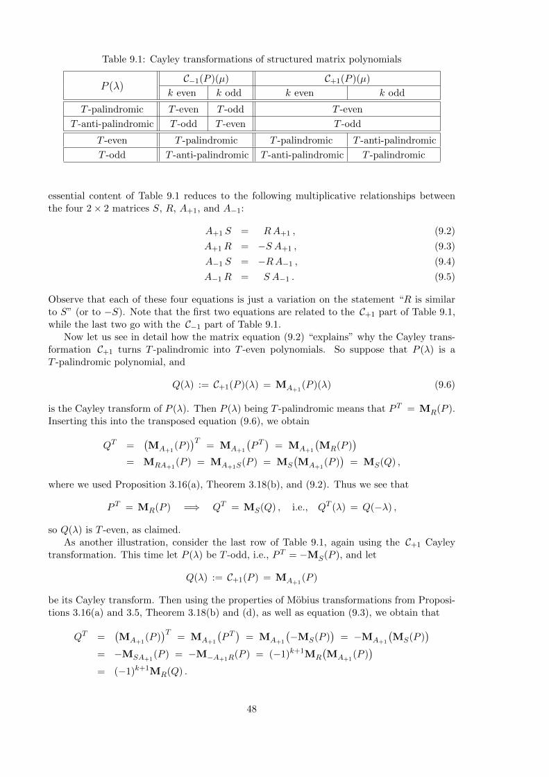
Table 9.1: Cayley transformations of structured matrix polynomials
C−1(P )(µ) C+1(P )(µ)P (λ)
k even k odd k even k odd
T -palindromic T -even T -odd T -even
T -anti-palindromic T -odd T -even T -odd
T -even T -palindromic T -palindromic T -anti-palindromic
T -odd T -anti-palindromic T -anti-palindromic T -palindromic
essential content of Table 9.1 reduces to the following multiplicative relationships betweenthe four 2× 2 matrices S, R, A+1, and A−1:
A+1 S = RA+1 , (9.2)
A+1R = −S A+1 , (9.3)
A−1 S = −RA−1 , (9.4)
A−1R = S A−1 . (9.5)
Observe that each of these four equations is just a variation on the statement “R is similarto S” (or to −S). Note that the first two equations are related to the C+1 part of Table 9.1,while the last two go with the C−1 part of Table 9.1.
Now let us see in detail how the matrix equation (9.2) “explains” why the Cayley trans-formation C+1 turns T -palindromic into T -even polynomials. So suppose that P (λ) is aT -palindromic polynomial, and
Q(λ) := C+1(P )(λ) = MA+1(P )(λ) (9.6)
is the Cayley transform of P (λ). Then P (λ) being T -palindromic means that P T = MR(P ).Inserting this into the transposed equation (9.6), we obtain
QT =(MA+1
(P ))T
= MA+1
(P T)
= MA+1
(MR(P )
)= MRA+1
(P ) = MA+1S(P ) = MS
(MA+1
(P ))
= MS(Q) ,
where we used Proposition 3.16(a), Theorem 3.18(b), and (9.2). Thus we see that
P T = MR(P ) =⇒ QT = MS(Q) , i.e., QT (λ) = Q(−λ) ,
so Q(λ) is T -even, as claimed.As another illustration, consider the last row of Table 9.1, again using the C+1 Cayley
transformation. This time let P (λ) be T -odd, i.e., P T = −MS(P ), and let
Q(λ) := C+1(P ) = MA+1(P )
be its Cayley transform. Then using the properties of Mobius transformations from Proposi-tions 3.16(a) and 3.5, Theorem 3.18(b) and (d), as well as equation (9.3), we obtain that
QT =(MA+1
(P ))T
= MA+1
(P T)
= MA+1
(−MS(P )
)= −MA+1
(MS(P )
)= −MSA+1
(P ) = −M−A+1R(P ) = (−1)k+1MR
(MA+1
(P ))
= (−1)k+1MR(Q) .
48
Thus we easily recover the T -anti-palindromicity ofQ when k is even, and the T -palindromicityof Q when k is odd. Analogous calculations produce all the other entries in Table 9.1.
In summary, then, the perspective afforded by our results about general Mobius trans-formations enables us to transparently see the Cayley connection between alternating andpalindromic structure as a straightforward consequence of simple relations between 2 × 2matrices.
10 Conclusions
The wide range of properties established in this paper for Mobius transformations actingon general matrix polynomials over an arbitrary field F make them a potent tool for bothdiscovering and proving nontrivial results.
Since a Mobius transformation can alter the degree of a polynomial, we have used poly-nomials of fixed grade as the domain of discourse. We can then view Mobius transformationsas a group of F-linear operators on a finite-dimensional vector space, and consequently de-velop a theory that is simpler and more unified than it would otherwise be. Many importanttransformations are now seen to be special instances of Mobius transformations.
We have shown that a number of structural features of matrix polynomials are preservedby Mobius transformations, for example, regularity, rank, minimal indices, the location ofzero entries, as well as symmetry and skew-symmetry. The relations of strict equivalence andspectral equivalence and the property of being a strong linearization or strong quadratificationare also preserved. Other important features like the determinant, Jordan characteristic,Smith form, invariant pairs and minimal bases have each been shown to change in a simpleand predictable way.
By linking palindromic and alternating matrix polynomials via Mobius transformations,the parallelism between the pairing conditions on their elementary divisors can be understoodand even predicted. Mobius transformations are thus shown to be an efficient device fortransferring results between matrix polynomial structures.
Finally, their role in yielding necessary and sufficient conditions for a given list of finiteand infinite elementary divisors to be realizable by a regular matrix polynomial highlights thepotential of Mobius transformations as effective tools for solving inverse polynomial eigenvalueproblems.
Acknowledgments
We thank the referee for many useful suggestions for improving the paper, and especially forcatching a mistake in the proof of Theorem 9.4.
References
[1] L.V. Ahlfors. Complex Analysis. McGraw-Hill, New York, 3rd edition, 1979.
[2] M. Al-Ammari and F. Tisseur. Hermitian matrix polynomials with real eigenvalues ofdefinite type. Part I: Classification. Linear Algebra Appl., 436:3954–3973, 2012.
[3] A. Amiraslani, R. M. Corless, and P. Lancaster. Linearization of matrix polynomialsexpressed in polynomial bases. IMA J. Numer. Anal., 29:141–157, 2009.
[4] A. Amparan, S. Marcaida, and I. Zaballa. An interpretation of Rosenbrock’s theorem vialocal rings. In Hassan Abid Yasser, editor, Linear Algebra - Theorems and Applications.InTech, 2012. DOI: 10.5772/46483. Available from:
49
http://www.intechopen.com/books/linear-algebra-theorems-and-applications/an-interpretation-of-rosenbrock-s-theorem-via-local-rings.
[5] A. Amparan, S. Marcaida, and I. Zaballa. On the structure invariants of proper rationalmatrices with prescribed finite poles. Linear Multilin. Algebra, 61:1464–1486, 2013.
[6] A. Amparan, S. Marcaida, and I. Zaballa. Finite and infinite structures of rationalmatrices: a local approach. Submitted for publication, 2014.
[7] K.J. Astrom. Computer Controlled Systems, Theory and Design. Prentice-Hall, Engle-wood Cliffs, New Jersey, second edition, 1999.
[8] J. Ball, I. Gohberg, and L. Rodman. Interpolation of rational matrix functions, volume 45of Operator Theory: Advances and Applications. Birkhauser, Basel, Switzerland, 1990.
[9] T. Betcke and D. Kressner. Perturbation, extraction and refinement of invariant pairsfor matrix polynomials. Linear Algebra Appl., 435:514–536, 2011.
[10] W.-J. Beyn and V. Thummler. Continuation of invariant subspaces for parameterizedquadratic eigenvalue problems. SIAM J. Matrix Anal. Appl., 31:1361–1381, 2009.
[11] D. Bini, B. Iannazzo, and B. Meini. Numerical Solution of Algebraic Riccati Equations.Fundamentals of Algorithms 09. SIAM, Philadelphia, PA, 2012.
[12] G. Birkhoff and S. MacLane. A Survey of Modern Algebra. MacMillan, New York, 2ndedition, 1953.
[13] R. Byers. Hamiltonian and Symplectic Algorithms for the Algebraic Riccati Equation.PhD thesis, Cornell University, Dept. Comp. Sci., Ithaca, NY, 1983.
[14] R. Byers, V. Mehrmann, and H. Xu. Trimmed linearizations for structured matrixpolynomials. Linear Algebra Appl., 429:2373–2400, 2008.
[15] I. Cabral and F. C. Silva. Unified theorems on completions of matrix pencils. LinearAlgebra Appl., 159:43–54, 1991.
[16] E. Chitambar, C. Miller, and Y. Shi. Matrix pencils and entanglement classification. J.Math. Physics, 51:072205, 2010.
[17] J. B. Conway. Functions of one complex variable. Springer-Verlag, New York, 2ndedition, 1978.
[18] R. M. Corless, N. Rezvani, and A. Amiraslani. Pseudospectra of matrix polynomialsthat are expressed in alternative bases. Math. in Computer Sci., 1:353–374, 2007.
[19] F. De Teran and F. Dopico. Sharp lower bounds for the dimension of linearizations ofmatrix polynomials. Electron. J. Linear Algebra, 17:518–531, 2008.
[20] F. De Teran, F. Dopico, and D. S. Mackey. Linearizations of singular matrix polynomialsand the recovery of minimal indices. Electron. J. Linear Algebra, 18:371–402, 2009.
[21] F. De Teran, F. Dopico, and D. S. Mackey. Fiedler companion linearizations and therecovery of minimal indices. SIAM J. Matrix Anal. Appl., 31:2181–2204, 2010.
[22] F. De Teran, F. Dopico, and D. S. Mackey. Fiedler companion linearizations for rectan-gular matrix polynomials. Linear Algebra Appl., 437:957–991, 2012.
50
[23] F. De Teran, F. Dopico, and D. S. Mackey. Spectral equivalence of matrix polynomi-als and the index sum theorem. To appear in Linear Algebra Appl. Also available asMIMS EPrint 2013.47, Manchester Institute for Mathematical Sciences, The Universityof Manchester, UK., 2013.
[24] J. Dion and C. Commault. Smith-McMillan factorizations at infinity of rational matrixfunctions and their control interpretation. Sys. Control Lett., 1:312–320, 1982.
[25] G. D. Forney. Minimal bases of rational vector spaces, with applications to multivariablelinear systems. SIAM J. Cont., 13:493–520, 1975.
[26] G. Frobenius. Theorie der linearen Formen mit ganzen Coefficienten. J. Reine Angew.Math. (Crelle), 86:146–208, 1878.
[27] F. R. Gantmacher. Theory of Matrices. Chelsea, New York, 1959.
[28] J. D. Gardiner and A. J. Laub. A generalization of the matrix-sign-function solution foralgebraic Riccati equations. Internat. J. Control, 44:823–832, 1986.
[29] I. Gohberg, M. A. Kaashoek, and P. Lancaster. General theory of regular matrix poly-nomials and band Toeplitz operators. Integral Equations Operator Theory, 11:776–882,1988.
[30] I. Gohberg, P. Lancaster, and L. Rodman. Matrix Polynomials. Academic Press, NewYork, 1982.
[31] C.-H. Guo, B. Iannazzo, and B. Meini. On the doubling algorithm for a (shifted) non-symmetric algebraic Riccati equation. SIAM J. Matrix Anal. Appl., 29:1083–1100, 2008.
[32] C.-H. Guo and W.-W. Lin. Solving a structured quadratic eigenvalue problem by astructure-preserving doubling algorithm. SIAM J. Matrix Anal. Appl., 31:2784–2801,2010.
[33] W. Hahn. Stability of Motion. Springer-Verlag, Heidelberg, 1967.
[34] E. Hairer, C. Lubich, and G. Wanner. Numerical Geometric Integration. Springer-Verlag,Heidelberg, 2002.
[35] N. J. Higham, D. S. Mackey, and F. Tisseur. Definite matrix polynomials and theirlinearizations by definite pencils. SIAM J. Matrix Anal. Appl., 31:478–502, 2009.
[36] D. Hinrichsen and A. J. Pritchard. Mathematical Systems Theory I: Modelling, StateSpace Analysis, Stability and Robustness. Springer-Verlag, Heidelberg, 2005.
[37] R. A. Horn and C. R. Johnson. Matrix Analysis. Cambridge University Press, Cambridge,1985.
[38] S. Johansson, B. Kagstrom, and P. Van Dooren. Stratification of full rank polynomialmatrices. Linear Algebra Appl., 439:1062–1090, 2013.
[39] B. Kagstrom and A. Ruhe, editors. Matrix Pencils, volume 973 of Lecture Notes in Math.Springer-Verlag, Berlin, 1983.
[40] P. Lancaster. Linearization of regular matrix polynomials. Electron. J. Linear Algebra,17:21–27, 2008.
51
[41] P. Lancaster and P. Psarrakos. A note on weak and strong linearizations of regular matrixpolynomials. MIMS EPrint 2006.72, Manchester Institute for Mathematical Sciences,The University of Manchester, UK, 2005.
[42] P. Lancaster and L. Rodman. The Algebraic Riccati Equation. Oxford University Press,Oxford, 1995.
[43] D.S. Mackey. Minimal indices and minimal bases via filtrations. MIMS EPrint 2012.82,Manchester Institute for Mathematical Sciences, The University of Manchester, UK,2012. Submitted for publication.
[44] D.S. Mackey, N. Mackey, C. Mehl, and V. Mehrmann. Structured polynomial eigen-value problems: Good vibrations from good linearizations. SIAM J. Matrix Anal. Appl.,28:1029–1051, 2006.
[45] D.S. Mackey, N. Mackey, C. Mehl, and V. Mehrmann. Vector spaces of linearizations formatrix polynomials. SIAM J. Matrix Anal. Appl., 28:971–1004, 2006.
[46] D.S. Mackey, N. Mackey, C. Mehl, and V. Mehrmann. Jordan structures of alternatingmatrix polynomials. Linear Algebra Appl., 432:867–891, 2010.
[47] D.S. Mackey, N. Mackey, C. Mehl, and V. Mehrmann. Smith forms for palindromicmatrix polynomials. Electron. J. Linear Algebra, 22:53–91, 2011.
[48] D.S. Mackey, N. Mackey, C. Mehl, and V. Mehrmann. Skew-symmetric matrix polyno-mials and their Smith forms. Linear Algebra Appl., 438:4625–4653, 2013.
[49] M. Marcus and H. Minc. A Survey of Matrix Theory and Matrix Inequalities. Allyn andBacon, Boston, 1964.
[50] V. Mehrmann. The Autonomous Linear Quadratic Control Problem, Theory and Nu-merical Solution. Number 163 in Lecture Notes in Control and Information Sciences.Springer-Verlag, Heidelberg, July 1991.
[51] V. Mehrmann. A step toward a unified treatment of continuous and discrete time controlproblems. Linear Algebra Appl., 241–243:749–779, 1996.
[52] V. Mehrmann and F. Poloni. A generalized structured doubling algorithm for the nu-merical solution of linear quadratic optimal control problems. Numer. Lin. Alg. Appl.,20:112–137, 2013.
[53] V. Noferini. The behaviour of the complete eigenstructure of a polynomial matrix undera generic rational transformation. Electron. J. Linear Algebra, 23:607–624, 2012.
[54] R. Ober and S. Montgomery-Smith. Bilinear transformation of infinite dimensional statespace systems and balanced realizations of nonrational transfer functions. SIAM J. Cont.Optim., 28:438–465, 1990.
[55] A. Oppenheim. Discrete Time Signal Processing. Pearson Higher Education, UpperSaddle River, New Jersey, third edition, 2010.
[56] G. Polya and G. Latta. Complex Variables. Wiley, New York, 1974.
[57] V. V. Prasolov. Problems and Theorems in Linear Algebra. American MathematicalSociety, Providence, 1994.
52
[58] R. Remmert. Theory of Complex Functions, volume 122 of Graduate Texts in Mathe-matics. Springer-Verlag, New York, 1991.
[59] V. Sima. Algorithms for Linear-Quadratic Optimization, volume 200 of Pure and AppliedMathematics. Marcel Dekker, Inc., New York, NY, 1996.
[60] G. W. Stewart. On the sensitivity of the eigenvalue problem Ax = λBx. SIAM J. Numer.Anal., 9(4):669–686, 1972.
[61] L. Taslaman, F. Tisseur, and I. Zaballa. Triangularizing matrix polynomials. LinearAlgebra Appl., 439:1679–1699, 2013.
[62] F. Tisseur and I. Zaballa. Triangularizing quadratic matrix polynomials. SIAM J. MatrixAnal. Appl., 34:312–337, 2013.
[63] K. Vahlen. Uber Bewegungen und complexe Zahlen. Math. Ann, 55:585–593, 1902.
[64] A. I. G. Vardulakis. Linear Multivariable Control. Wiley, New York, 1991.
[65] H. K. Wimmer. The structure of nonsingular polynomial matrices. Math. SystemsTheory, 14:367–379, 1981.
[66] I. Zaballa and F. Tisseur. Finite and infinite elementary divisors of matrix polynomials: aglobal approach. MIMS EPrint 2012.78, Manchester Institute for Mathematical Sciences,The University of Manchester, UK, 2012.
53


![Some applications of the spectral theory of …1.1 Hyperbolic geometry and M¨obius transformations This overview takes most of its inspiration from [9], [10] and [11]. Throughout](https://img.pdfslide.net/doc/110x75/5ecafbd3e7aa29671b3b2909/some-applications-of-the-spectral-theory-of-11-hyperbolic-geometry-and-mobius.jpg)