m ul reentry capsul aero dynami sti cal si m ul ati on of reentry capsul e aero dynami cs i n hyp ersoni c near-conti n uum ﬂows Mikhail S. Ivanov Computational Aerodynamics Laboratory,

Stati sti cal si mul ati on of reentry capsul e aero dynami cs

i n hyp ersoni c near-conti nuum flows

Mikhail S. IvanovComputational Aerodynamics Laboratory,

Khristianovich Institute of Theoretical and Applied Mechanics (ITAM),Siberian Branch of the Russian Academy of Sciences,

Institutskaya 4/1, Novosibirsk 630090, Russia

24-28 January 2011

Summary

Current challenges and problems pertaining to the development and application of theDSMC method for high-altitude aerodynamics are discussed. Attention is paid to issuesrelated to the efficiency and accuracy of the method in the near-continuum regime, aswell as its use for modeling of rarefied flows with real gas effects. Accurate predictionof force and heat aerodynamic characteristics of reentry vehicles and spacecraft requirescomprehensive investigation of hypersonic flows in the near-continuum regime. A pow-erful software system SMILE, which uses the direct simulation Monte Carlo method asa numerical approach and is built basing on the contemporary knowledge in this field,is developed to solve advanced problems of high-altitude aerothermodynamics. Effectivenumerical algorithms and physically grounded models of real gas effects are implementedin SMILE. Aerodynamics of promising reentry capsule in the near-continuum regime isconsidered as an example.

RTO-EN-AVT-194 18 - 1

Report Documentation Page Form ApprovedOMB No. 0704-0188

Public reporting burden for the collection of information is estimated to average 1 hour per response, including the time for reviewing instructions, searching existing data sources, gathering andmaintaining the data needed, and completing and reviewing the collection of information. Send comments regarding this burden estimate or any other aspect of this collection of information,including suggestions for reducing this burden, to Washington Headquarters Services, Directorate for Information Operations and Reports, 1215 Jefferson Davis Highway, Suite 1204, ArlingtonVA 22202-4302. Respondents should be aware that notwithstanding any other provision of law, no person shall be subject to a penalty for failing to comply with a collection of information if itdoes not display a currently valid OMB control number.

1. REPORT DATE JAN 2011

2. REPORT TYPE N/A

3. DATES COVERED -

4. TITLE AND SUBTITLE Statistical simulation of reentry capsule aerodynamics in hypersonicnear-continuum flows

5a. CONTRACT NUMBER

5b. GRANT NUMBER

5c. PROGRAM ELEMENT NUMBER

6. AUTHOR(S) 5d. PROJECT NUMBER

5e. TASK NUMBER

5f. WORK UNIT NUMBER

7. PERFORMING ORGANIZATION NAME(S) AND ADDRESS(ES) Computational Aerodynamics Laboratory, Khristianovich Institute ofTheoretical and Applied Mechanics (ITAM), Siberian Branch of theRussian Academy of Sciences, Institutskaya 4/1, Novosibirsk 630090, Russia

8. PERFORMING ORGANIZATIONREPORT NUMBER

9. SPONSORING/MONITORING AGENCY NAME(S) AND ADDRESS(ES) 10. SPONSOR/MONITOR’S ACRONYM(S)

11. SPONSOR/MONITOR’S REPORT NUMBER(S)

12. DISTRIBUTION/AVAILABILITY STATEMENT Approved for public release, distribution unlimited

13. SUPPLEMENTARY NOTES See also ADA579248. Models and Computational Methods for Rarefied Flows (Modeles et methodes decalcul des coulements de gaz rarefies). RTO-EN-AVT-194

14. ABSTRACT Current challenges and problems pertaining to the development and application of the DSMC method forhigh-altitude aerodynamics are discussed. Attention is paid to issues related to the efficiency and accuracyof the method in the near-continuum regime, as well as its use for modeling of rarefied flows with real gaseffects. Accurate prediction of force and heat aerodynamic characteristics of reentry vehicles andspacecraft requires comprehensive investigation of hypersonic flows in the near-continuum regime. Apowerful software system SMILE, which uses the direct simulation Monte Carlo method as a numericalapproach and is built basing on the contemporary knowledge in this field, is developed to solve advancedproblems of high-altitude aerothermodynamics. Effective numerical algorithms and physically groundedmodels of real gas effects are implemented in SMILE. Aerodynamics of promising reentry capsule in thenear-continuum regime is considered as an example.

15. SUBJECT TERMS

16. SECURITY CLASSIFICATION OF: 17. LIMITATION OF ABSTRACT

SAR

18. NUMBEROF PAGES

38

19a. NAME OFRESPONSIBLE PERSON

a. REPORT unclassified

b. ABSTRACT unclassified

c. THIS PAGE unclassified

Standard Form 298 (Rev. 8-98) Prescribed by ANSI Std Z39-18

CONTENTS CONTENTS

Contents

1 Introduction 3

2 Conceptual issues of the DSMC method 4

3 Real gas effect models for DSMC 6

4 DSMC versus continuum CFD 9

5 Numerical accuracy of the DSMC method 11

6 High-altitude aerothermodynamics of a promising capsule 14

7 Prospects for the DSMC method 20

8 Acknowledgments 20

A Appendix 1. Majorant collision frequency schemes 21

A Appendix 2. Gas/surface interaction models 31

References 35

18 - 2 RTO-EN-AVT-194

1 INTRODUCTION

1 Introduction

The study of physical phenomena in rarefied nonequilibrium flows is a challengingproblem directly related to the development of new aerospace technologies. Rarefied gasdynamics, that deals with these phenomena, is the synthesis of a great number of funda-mental problems such as molecular collision dynamics and energy transfer phenomena incollisions, gas-surface interactions, condensation and evaporation, plume and expansionflows, and many others. All these problems are in close connection with applied, prac-tical issues that can be conventionally divided into two groups. The first group coversthe questions related to aerodynamic calculations of hypersonic flight of vehicles at highaltitudes, the second group being mainly represented by the problems that involve thecalculation of nozzle flows in thrusters and jets exhausting into vacuum and interactingwith the surface of space objects.

Substantial difficulties arising in the study of such flows are caused by both the prob-lems related to rarefaction and physico-chemical effects. It is commonly known thatexperimental simulation of nonequilibrium low-density flows is rather problematic andexpensive. The difficulties of experimental modeling have stimulated an intense develop-ment of various approaches for numerical simulation of these flows. Presently there arenumerous numerical approaches for solving the problems of rarefied gas dynamics, andthe choice of this or that approach depends usually on the flow rarefaction, the problemdimension and the presence of real gas effects.

The choice of the numerical approach to be used to model rarefied nonequilibriumflows greatly depends on the extent of flow rarefaction. For near-continuum flows, it isusually sufficient to take into account the initial effects of rarefaction through the bound-ary conditions of slip velocity and temperature jump on the surface. The Navier-Stokesor viscous shock layer equations are commonly used with these boundary conditions. TheNavier-Stokes equations can be derived from the Boltzmann equation under the assump-tion of small deviation of the distribution function from equilibrium. Therefore, theybecome unsuitable for studying rarefied flows where the distribution function becomesconsiderably nonequilibrium.

To study rarefied flows with a significant degree of nonequilibrium, the Direct Simu-lation Monte Carlo (DSMC) method is usually employed. This method has become themain technique for studying complex multidimensional rarefied flows. It has been success-fully applied over the last four decades to model various flow phenomena and gas dynamicproblems. The method has gradually evolved to the stage where its application to cal-culate complex three- dimensional flows is almost straightforward. The extended area ofapplicability of the DSMC method is from the near-continuum regime where it overlapswith that of the continuum approaches, to the free-molecular regime. In practice, theDSMC method is computationally intensive compared with its continuum counterparts.However, with increasing capabilities of modern parallel computers this method acquiresnew areas of application, such as modeling of internal and external near-continuum flows,detailed study of different three-dimensional problems with real gas effects, and others.

The Laboratory of Computational Aerodynamics from the Khristianovich Institute ofTheoretical and Applied Mechanics of the Siberian Branch of the Russian Academy ofSciences has more than decade-long experience in the development of the DSMC method.

RTO-EN-AVT-194 18 - 3

2 CONCEPTUAL ISSUES OF THE DSMC METHOD

The result of these efforts is a computational system called SMILE (Statistical ModelingIn Low-Density Environment) capable of solving a very wide range of basic and appliedproblems. The SMILE system provides a complete lifecycle of computations starting froma geometry model, pre-processing, going through the computation proper, and finishingwith post-processing and presentation of results. All SMILE subsystems have a GraphicUser Interface (GUI), which makes them user-friendly and easy to use. The SMILEcore code is written in FORTRAN90 and has no memory limitations specific to staticFORTRAN programs. The user interface of the system is written in C++ and uses afree cross-platform wxWidgets GUI library. The same theoretical basis (majorant colli-sion frequency schemes) is used to develop more advanced software systems RGDAS andSMILE++.

The principal objectives of the paper are to analyze the modern status of the DSMCmethod, outline promising directions of method development, discuss problems that maybe encountered, and give possible ways to overcome these problems. The paper discussesmodeling of real gas effects, the numerical accuracy issues for the DSMC method, andapplication of the SMILE software system for studying promising capsule aerodynamics.

2 Conceptual issues of the DSMC method

The DSMC method is traditionally considered as a method of statistical simulationof the behavior of a great number of simulated gas molecules. Usually the number ofsimulated particles is large enough (∼ 105 − 108), but this is extremely small in com-parison with the number of real molecules. Each simulated particle is then regarded asrepresenting an appropriate number of actual molecules, Fnum.

The main principle of DSMC is the splitting of continuous process of molecular motionand collisions into two successive stages at the time step ∆t. The computational domainis divided into cells of size ∆x such that the variation of the flow parameters in every cellis small. The time step ∆t should be small as compared with the mean collision time τλ.Free motion of molecules and their collisions are considered successively at this time step∆t:

1. Collisions of particles belonging to the given cell in each cell of are carried out inde-pendently in each cell of physical space, i.e. the collisions of particles in the neighboringcells are not considered. Since the distribution function variation is supposed small in thecell, when a pair of particles for collision is chosen the relative distance between them isnot taken into account. The post-collision velocities are calculated in accordance with theconservation laws of linear momentum and energy.

2. All molecules located in the computational domain are displaced by the distancedetermined by their velocities at the moment and by the time step ∆t. If a molecule leavesthe computational domain, then its velocity is recomputed according to the boundaryconditions. At the same step ∆t new particles entering the computational domain aregenerated in accordance with the distribution function specified at the domain boundaries.

Thus, the following principals steps are specified in the DSMC procedure:

• entering new molecules

18 - 4 RTO-EN-AVT-194

2 CONCEPTUAL ISSUES OF THE DSMC METHOD

• molecular motion

• gas/surface collisions

• indexing of molecules over collision cells

• collisions

• sampling of macroparameters

After finishing computation, the results of computations are processed to obtain theflowfields of gas dynamics parameters, total and distributed surface quantities. The mainsteps of the DSMC technique are discussed below.

The state of each simulated particle is characterized by its coordinate r and velocityv. The state of the whole system of N particles is described by a 6N -dimensional vector{R, V } = {r1, v1, ..., rN , vN}. The evolution of such a system can be represented as ajump-like motion of a point in the 6N -dimensional phase space. The DSMC method canbe then treated as statistical simulation of the 6N -dimensional random jump-like process.

In the traditional approach Bird [1] of constructing numerical schemes of the DSMCmethod, the description of procedures for trajectory simulation of the random process isbased on physical concepts of rarefied gas and on physical assumptions that create thebasis for the phenomenological derivation of the Boltzmann equation.

A different approach was proposed by Ivanov and Rogasinsky [2] who constructednumerical schemes for simulating a 6N -dimensional, continuous in time, random processof spatially nonuniform evolution of a system of N particles. Majorant collision frequency(MCF) schemes of the DSMC method were derived from the Kac [3] and Leontovich[4] master kinetic equations (MKE). This is a linear integro-differential equation thatdescribes the time behavior of an N -particle gas model with binary collisions on the levelof the N -particle distribution function fN . The linear MKE may be transformed intothe nonlinear Boltzmann equation when N → ∞ and the molecular chaos condition issatisfied (see, e.g., [5]). Since a finite number of simulated particles is used in the DSMCsimulations, it is natural to directly use MKE for constructing numerical schemes of theDSMC method. The procedure of constructing MCF schemes is described in detail inAppendix 1.

The extension of the majorant collision frequency schemes obtained from MKE to thecase of multispecies chemically reacting mixtures is straightforward. It implies the changein cross-sections of the corresponding inelastic processes and, hence, the change in thecollision algorithm only in the part that is related to the collision mechanics.

The procedures of modeling gas-surface interaction for two reflection models (specular-diffuse and Nocilla models) can be found in Appendix 2.

Currently used numerical schemes of the DSMC method (NTC [1], NCT [6], MCF [2,7]) are very close both in terms of efficiency and numerical implementation. At present,there are no essential internal resources for increasing the efficiency of the collision stageof the DSMC method. The main effort in improving the method efficiency is directed tothe study of influence of the grid type, the use of multi-zone approaches, variable timestep, grid adaption procedures, etc [8,9,38].

RTO-EN-AVT-194 18 - 5

3 REAL GAS EFFECT MODELS FOR DSMC

3 Real gas effect models for DSMC

An accurate prediction of high-temperature rarefied flows, such as those behind theshock wave formed about a space vehicle at high altitudes, requires the use of adequatemodels of physical and chemical processes - so-called real gas effects, and effective numer-ical procedures. An example of the impact of these processes on the flow is given in Fig.1 where the translational temperature fields about the Soyuz capsule at an altitude of 85km are shown for nonreacting and reacting gases [9].

Two most important effects of chemical reactions are the decrease in temperature inthe shock front and a smaller shock stand-off distance. In conventional continuum gas

Figure 1: Translational temperature fields about a reentry capsule, al-titude 85 km, velocity 8 km/s. Nonreacting (left) and reacting (right)air.

dynamics the real gas effects are usually understood as such high-temperature phenomenaas molecular vibration, dissociation, ionization, surface chemical reactions, and radiation.In describing the problems of rarefied gas dynamics, with a typical large, often of theorder of the reference flow scale, shock wave width and rarefaction effects exerting thedetermining effect on the flow structure, it is convenient to consider the “real gas effects”in a wider sense. As applied to kinetic methods based on the microscopic approach andused for studying RGD problems, it seems natural to relate the real gas effects with allphenomena associated with molecular collisions, namely, molecular interaction potential,rotational degrees of freedom, vibrational degrees of freedom, chemical reactions in gas,ionization, and radiation.

One of the most challenging problems remaining in terms of the method developmentand improvement is related to the need to effectively and reliably simulate processes ofenergy transfer between internal and translational modes, chemical reactions, ionization,and radiation. The presence of one or more of these processes drastically changes flowproperties such as density and temperature, and the development of adequate models istherefore very important. A number of DSMC techniques and models were suggested

18 - 6 RTO-EN-AVT-194


and used in the last decade that cover different aspects of the problem (see, for example,Refs. [10]-[14] and references therein). Currently, there is a lack of models that aregeneral enough to treat various molecular interactions and processes, sufficiently accurateto capture complex flow physics, easy to implement, and computationally efficient to beapplied to calculate near-continuum flows.

In what follows we would like to mention the collision models that are both compu-tationally efficient, easy to implement, and sufficiently general to be applied for any typeof interactions between atoms and diatomic and polyatomic molecules. The Variable SoftSphere (VSS) model [15] is one of the most widely used models of intermolecular inter-action. In this model the total collision cross-section depends on the relative collisionvelocity, and two parameters of the model are determined from the condition of coinci-dence of diffusion and viscous cross-sections of the VSS and the inverse-power potentialmodels. Even though the model does not include the attractive part of the potential, it isapplicable for most conditions where the DSMC is used. Rotational energy distributionis conventionally assumed to be continuous, which makes the energy transfer algorithmssimpler, especially for polyatomic molecules.

The discrete description was suggested in [16] for different types of polyatomic molecules.The traditional Larsen-Borgnakke (LB) model [17] is most widely used in the DSMCmethod to describe the energy exchange between the translational and rotational modesof colliding particles. In this model, the energy spectrum of rotational mode is assumedcontinuous, and some fraction ϕ = 1/ZR of the total number of collisions takes placewith the energy exchange between translational and rotational degrees of freedom. Thepost-collision rotational and relative translational energies are simulated in accordancewith the local equilibrium distribution functions and are proportional to the number ofdegrees of freedom of the mode. Several improvements were suggested for the LB modelto make the rotational relaxation rate in the DSMC modeling correspond to the contin-uum and experimental rates. First, temperature-dependent rotational collision numberwas suggested [12]. Then, a correction factor was derived that establishes a relation ofZR employed in the DSMC method with a continuum analog used in the Jeans relax-ation equation [18]. Finally, a particle selection methodology was proposed [19], whichprohibits multiple relaxation events during a single collision, and matches Jeans equationfor general gas mixtures. In contrast to the traditional LB model, the particle selectionmethodology prohibiting multiple relaxation events does not include directly rotational-rotational energy transfer. Note that this type of energy transfer has not been studiedseparately in the DSMC method. Since the translational-rotational energy transfer is fast,and rotational distribution is usually less important for chemical reactions and radiativeprocesses than vibrational distribution, accurate modeling of the translational-rotationalenergy transfer is sufficient for most cases.

The spacing between rotational energy levels is small, and the continuum model of ro-tational mode approximates well the discrete distribution [20]. It is therefore reasonable touse the continuum Larsen-Borgnakke model with the temperature-dependent relaxationnumber, the correction factor [18] and a selection methodology that prohibits multiplerelaxation events. Two models for the vibrational energy distributions, continuous anddiscrete, are traditionally used in the DSMC method. Generally, the continuity of thevibrational energy mode may be a too rough allowance, since the vibrational spectrum ofreal molecules is characterized by large gaps between the neighboring energy levels. Be-

RTO-EN-AVT-194 18 - 7


sides the physical reason, there are several numerical problems connected with the use ofthe continuum vibrational energy spectra. These are the need for special cut-off parame-ters for the LB model when the number of vibrational degrees of freedom is less than two,additional assumptions that have to be used in the LB collision energy transfer modeling,and an inaccurate shape of the internal energy distribution functions at equilibrium [20].The last point is important for reactions whose cross-sections directly depend on vibra-tional states (such as vibrationally favored reactions). Also, internal energy distributionstrongly affects the flow radiation. The discrete internal energy model does not have thesedrawbacks, but requires a special correction procedure to be used for the chemical reac-tion rates to follow the experimental rates expressed in the Arrhenius form. Many discretemodels for the translation-vibration energy transfer were suggested in the literature. Theydiffer considerably in the way of determining the vibrationally inelastic cross-sections. Adiscrete version of the LB model is presented in [21]. In the model [22], the probabilityof VT transitions is determined using the inverse Laplace transformation for a simpleharmonic oscillator from the temperature-dependent relaxation rate [23]. The approach[24] is based on the use of the information theory for determining post-collision states. Inthe model [25] the cross-sections for vibration-translation transitions are used, obtainedfor an anharmonic oscillator from a quasi-classical approximation of the scattering theory.

The vibration-vibration energy transfer was also modeled in the DSMC method. Wemention here the model [26] where both vibration-translation and vibration-vibrationtransitions for a simple harmonic oscillator have been considered. The vibration-vibrationenergy exchange model based on the quasiclassical approach was developed in [25]. Thisenergy transfer process was found to be important for the vibrational populations inhypersonic flows at high altitudes. All these and many other models have been developedonly for diatomic molecules. Because of this, it seems most reasonable at present touse the LB model with particle selection. Temperature-dependent vibrational relaxationrate has to be specified using vibrational mode characteristic temperatures of polyatomicmolecules. A correction factor [27] has to be used that enables one to match the vibrationalrelaxation rates in the DSMC modeling to the relaxation rate given by the Landau-Tellerequation. Note that the LB model was not yet applied to vibration-vibration energytransfer. Such an application would require to specify the corresponding collision numbersthat may not be known for many molecular systems.

The DSMC method has been used for calculating rarefied hypersonic chemically re-acting flows for more than two decades. The major problem in generating the modelof chemical reactions is the determination of energy-dependent cross-sections of chemi-cal reactions. Note here that the temperature dependences of chemical reaction rates,traditional for the continuum approach, cannot be applied to the DSMC method, andenergy-dependent reaction cross-sections have to be used. As the exact expressions forthese cross-sections are not available now even for simple dissociation reactions in air,some approximations have to be employed. The first simplistic models have been replacedby the total collision energy (TCE) model [28] built on the basis of collision theory forchemical reactions. This model is efficient and is used presently for calculating two- andthree-dimensional flows. It employs the major assumption that the reaction probabilitydepends on the total collision energy. A specific form of this dependence is assumed thatallows analytic determination of unknown coefficients. The derivation uses the reactionrate coefficient in Arrhenius form and the Hinshelwood expression for the equilibrium en-

18 - 8 RTO-EN-AVT-194

4 DSMC VERSUS CONTINUUM CFD

ergy distribution function that implies continuous distribution of internal modes [28]. Theproblems inherent in continuous vibrational energy models that were discussed above leadto the conclusion that the use of discrete models in the DSMC method is preferable. Oneproblem related to the use of discrete energy levels is that the existing chemical reactionmodels derived for continuous internal energies need special modifications to be appliedfor discrete energies. In this case, a correction procedure is necessary for the reaction ratesin the DSMC method match available experimental data. Such a correction procedurewas developed in [20]. It utilizes a Monte Carlo approach to find modified constants inthe reaction cross-section energy dependence, the use of which enables one to match theoriginal reaction rates at equilibrium.

The procedure is applied to the total collision energy model, but is generally applicableto any reaction model based on the collision theory for chemical reactions. Several modelsthat include a direct dependence of the reaction cross-sections on the collider vibrationalenergy (so-called vibration-dissociation coupling) were proposed earlier [10, 13, 14]. Thedeficiency of these models is that they imply some fixed or variable parameters thatdetermine the extent of vibrational favoring. These parameters are extracted or verifiedthrough comparison with available experimental data. Note that some reactions may nothave vibrational favoring, and therefore the model [28] may turn to be reasonable [29].

4 DSMC versus continuum CFD

The areas where the continuum and kinetic approaches are currently applied over-lap in the regime of low Knudsen numbers. The recent experimental and computationalactivity related to accurate prediction of laminar flow separation in the near-continuumregime shows that even for non-reacting gases there are still problems of validation andverification of numerical approaches that need to be resolved. Numerical analysis of suchflows is traditionally performed using Navier-Stokes (NS) equations, with the initial ef-fects of rarefaction taken into account through the slip velocity and temperature jump.The use of slip conditions is caused by the fact that rarefaction effects can be observedfor slender bodies even for rather high Reynolds numbers (Re = 20, 000 − 30, 000). Thestate-of-the-art algorithms of the DSMC method (adaptive grids, variable time step, etc.)allow one to simulate flows at such high Reynolds numbers. This makes realistic thestudy of the applicability area of the continuum approach to model laminar separatedflows. The study was started in [30] and continued in [31] where a detailed numericalmodeling of an axisymmetric shock wave / laminar boundary layer interaction was per-formed by the continuum (NS) and kinetic (DSMC) approaches for the ONERA R5Chwind tunnel conditions. The DSMC results showed the presence of a high slip velocityand temperature jump near the wall. The application of slip conditions for the NS solverhas a substantial effect on the entire flow field and allows one to decrease the differencebetween the continuum and DSMC results. The left part of Fig. 2 shows that the profileof the gas velocity at the wall Ug obtained by the DSMC method is in excellent agreementwith the Ug profile calculated from the NS slip velocity using the solution for the velocitydistribution across the Knudsen layer [32]. However, the NS solver with slip conditionspredicts a larger length of the separation region than the DSMC method. To eliminate

RTO-EN-AVT-194 18 - 9

4 DSMC VERSUS CONTINUUM CFD

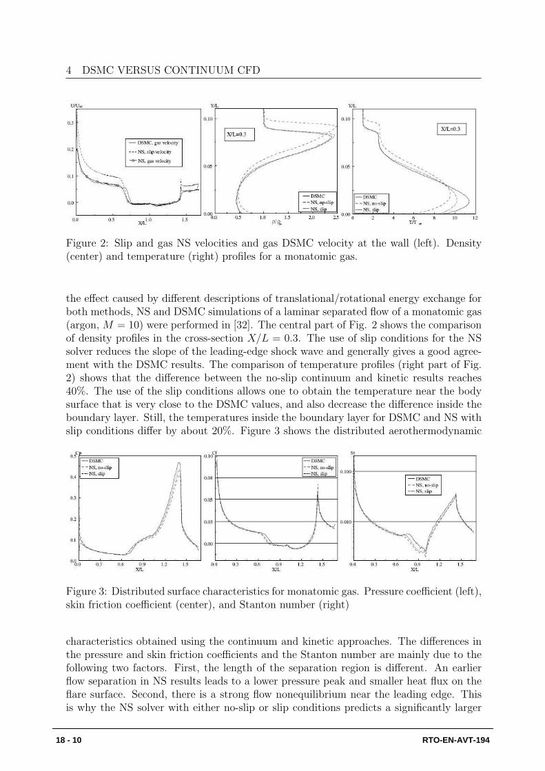
Figure 2: Slip and gas NS velocities and gas DSMC velocity at the wall (left). Density(center) and temperature (right) profiles for a monatomic gas.

the effect caused by different descriptions of translational/rotational energy exchange forboth methods, NS and DSMC simulations of a laminar separated flow of a monatomic gas(argon, M = 10) were performed in [32]. The central part of Fig. 2 shows the comparisonof density profiles in the cross-section X/L = 0.3. The use of slip conditions for the NSsolver reduces the slope of the leading-edge shock wave and generally gives a good agree-ment with the DSMC results. The comparison of temperature profiles (right part of Fig.2) shows that the difference between the no-slip continuum and kinetic results reaches40%. The use of the slip conditions allows one to obtain the temperature near the bodysurface that is very close to the DSMC values, and also decrease the difference inside theboundary layer. Still, the temperatures inside the boundary layer for DSMC and NS withslip conditions differ by about 20%. Figure 3 shows the distributed aerothermodynamic

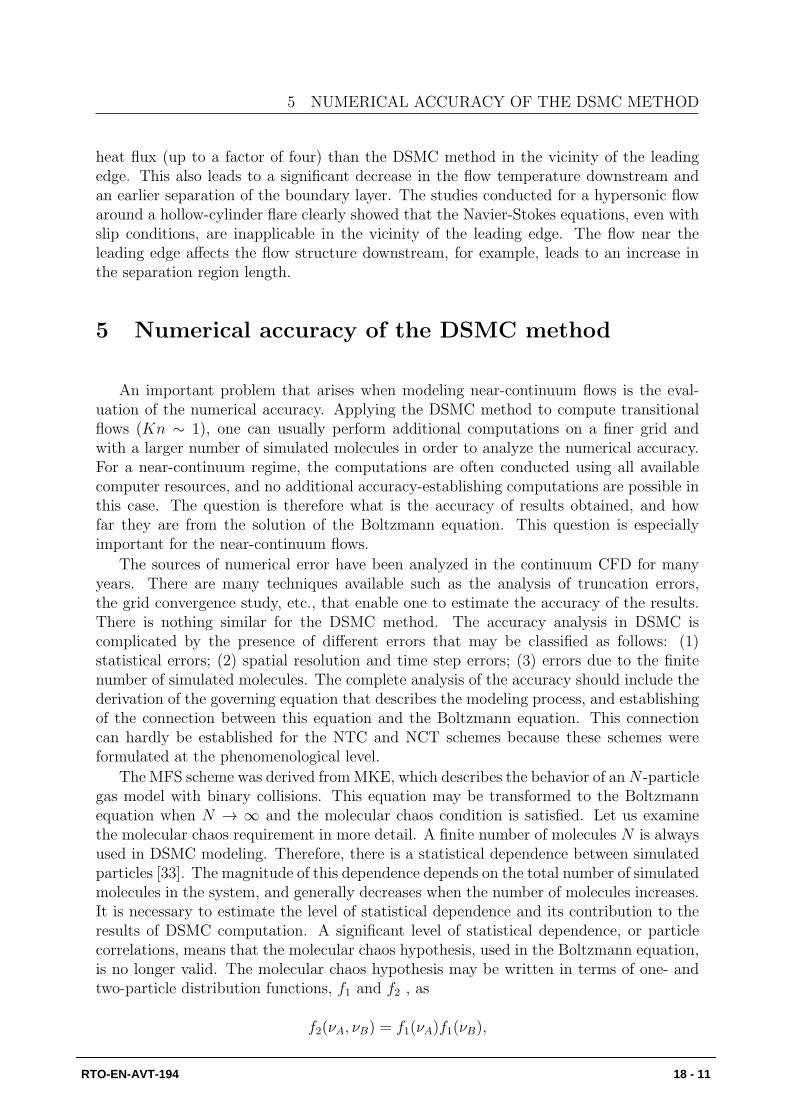
Figure 3: Distributed surface characteristics for monatomic gas. Pressure coefficient (left),skin friction coefficient (center), and Stanton number (right)

characteristics obtained using the continuum and kinetic approaches. The differences inthe pressure and skin friction coefficients and the Stanton number are mainly due to thefollowing two factors. First, the length of the separation region is different. An earlierflow separation in NS results leads to a lower pressure peak and smaller heat flux on theflare surface. Second, there is a strong flow nonequilibrium near the leading edge. Thisis why the NS solver with either no-slip or slip conditions predicts a significantly larger

18 - 10 RTO-EN-AVT-194

5 NUMERICAL ACCURACY OF THE DSMC METHOD

heat flux (up to a factor of four) than the DSMC method in the vicinity of the leadingedge. This also leads to a significant decrease in the flow temperature downstream andan earlier separation of the boundary layer. The studies conducted for a hypersonic flowaround a hollow-cylinder flare clearly showed that the Navier-Stokes equations, even withslip conditions, are inapplicable in the vicinity of the leading edge. The flow near theleading edge affects the flow structure downstream, for example, leads to an increase inthe separation region length.

5 Numerical accuracy of the DSMC method

An important problem that arises when modeling near-continuum flows is the eval-uation of the numerical accuracy. Applying the DSMC method to compute transitionalflows (Kn ∼ 1), one can usually perform additional computations on a finer grid andwith a larger number of simulated molecules in order to analyze the numerical accuracy.For a near-continuum regime, the computations are often conducted using all availablecomputer resources, and no additional accuracy-establishing computations are possible inthis case. The question is therefore what is the accuracy of results obtained, and howfar they are from the solution of the Boltzmann equation. This question is especiallyimportant for the near-continuum flows.

The sources of numerical error have been analyzed in the continuum CFD for manyyears. There are many techniques available such as the analysis of truncation errors,the grid convergence study, etc., that enable one to estimate the accuracy of the results.There is nothing similar for the DSMC method. The accuracy analysis in DSMC iscomplicated by the presence of different errors that may be classified as follows: (1)statistical errors; (2) spatial resolution and time step errors; (3) errors due to the finitenumber of simulated molecules. The complete analysis of the accuracy should include thederivation of the governing equation that describes the modeling process, and establishingof the connection between this equation and the Boltzmann equation. This connectioncan hardly be established for the NTC and NCT schemes because these schemes wereformulated at the phenomenological level.

The MFS scheme was derived fromMKE, which describes the behavior of anN -particlegas model with binary collisions. This equation may be transformed to the Boltzmannequation when N → ∞ and the molecular chaos condition is satisfied. Let us examinethe molecular chaos requirement in more detail. A finite number of molecules N is alwaysused in DSMC modeling. Therefore, there is a statistical dependence between simulatedparticles [33]. The magnitude of this dependence depends on the total number of simulatedmolecules in the system, and generally decreases when the number of molecules increases.It is necessary to estimate the level of statistical dependence and its contribution to theresults of DSMC computation. A significant level of statistical dependence, or particlecorrelations, means that the molecular chaos hypothesis, used in the Boltzmann equation,is no longer valid. The molecular chaos hypothesis may be written in terms of one- andtwo-particle distribution functions, f1 and f2 , as

f2(νA, νB) = f1(νA)f1(νB),

RTO-EN-AVT-194 18 - 11


where νA and νB are the velocities of the two collision partners, A and B. For somefunction of velocity, h ≡ h(ν), we can write

∫ ∞

−∞

f2(νA, νB)h(νA)h(νB)dνAdνB =

∫ ∞

−∞

f1(νA)h(νA)dνA

∫ ∞

−∞

f1(νB)h(νB)dνB

This expression may be rewritten as

〈h(νA)h(νB)〉 = 〈h(νA)〉〈h(νB)〉

where 〈...〉 denotes averaging. As was mentioned above, the molecular chaos hypothesis isnot strictly valid for a finite number of particles, which means that the above expressiondoes not hold. Let us introduce the following correlator G2,

G2 =〈h(νA)h(νB)〉〈h(νA)〉〈h(νB)〉

− 1

Obviously, this correlator may serve as an indicator of the presence of molecular corre-lations. The smaller the correlations, the closer G2 is to 0. The value of G2 may bedirectly calculated in the DSMC method over all cells in the computational domain, andh(ν) = V 2

x is usually used for this purpose [34], [35]. An additional criterion that allowsfor a practical verification of the presence of the statistical dependence between simu-lated particles is the relative number of repeated collisions [34]. Repeated collisions arecollisions between the same pair of particles during their lifetime in the computationaldomain. The number of repeated collisions is directly related to the number of particlesNλ in a volume with the linear size equal to the local mean free path. If Nλ > 1, one cansay that the simulation results are close to the solution of the Boltzmann equation. Let

Figure 4: 1D shock wave, monatomic gas. Density n and parallel temperature Tx (left).Correlator G2(V 2

x ) and repeated collision fraction (right).

us consider a 1D shock wave structure as an example where the G2 correlator and therepeated collision number are used. A monatomic gas of hard sphere molecules is usedwith M = 8. The computational domain was 15 upstream mean free paths. Three caseswere considered here. 20 particles in the upstream cells was used in Case 1 (baseline case),

18 - 12 RTO-EN-AVT-194


with the cell size L of 0.25 of the upstream mean free path λ. For Case 2, 2 particles perupstream cell was used with L = 0.25λ. The number of particles for case 3 was the sameas in Case 1, but L = 0.00625λ. The average number of particles in the upstream cellswas therefore 0.5 in this case.

The density and parallel temperature distributions inside the shock wave are shownin Fig. 4 (left). The profiles are very similar for Cases 1 and 3, and somewhat differentfor Case 2. The G2 correlator and repeated collision fraction are given in Fig. 4 (right).For Case 1, the values of G2 are close to zero, being less than 0.01 even in the regionof strong nonequilibrium, and the number of repeated collisions is not greater than 2percent of the total number of collisions. The values of the correlator and repeatedcollision fraction increase about ten times for Case 2 compared to case 1, even though thecollision frequency is the same since the MFS scheme is used. The increase in the particlestatistical correlations is the reason for the difference in the macroparameters observedin Fig. 4 (left). Obviously, the difference is due to the decrease in the total number ofsimulated particles in the computational domain. We can therefore state that an accuratecalculation of the collision frequency in a cell is not sufficient for obtaining an accurateresult. An interesting fact is that the reduction of the cell size while preserving the totalnumber of molecules (Cases 1 and 3) does not change macroparameters and only slightlychanges the correlator and the number of repeated collisions. This shows that the numberof particles in cell is not a determining factor for MFS. The important parameters are thetotal number of particles in the system and Nλ.

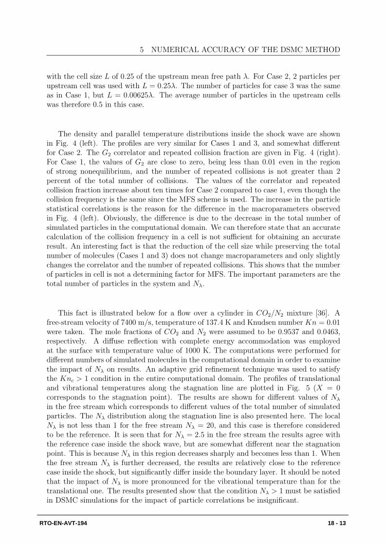
This fact is illustrated below for a flow over a cylinder in CO2/N2 mixture [36]. Afree-stream velocity of 7400 m/s, temperature of 137.4 K and Knudsen number Kn = 0.01were taken. The mole fractions of CO2 and N2 were assumed to be 0.9537 and 0.0463,respectively. A diffuse reflection with complete energy accommodation was employedat the surface with temperature value of 1000 K. The computations were performed fordifferent numbers of simulated molecules in the computational domain in order to examinethe impact of Nλ on results. An adaptive grid refinement technique was used to satisfythe Knc > 1 condition in the entire computational domain. The profiles of translationaland vibrational temperatures along the stagnation line are plotted in Fig. 5 (X = 0corresponds to the stagnation point). The results are shown for different values of Nλ

in the free stream which corresponds to different values of the total number of simulatedparticles. The Nλ distribution along the stagnation line is also presented here. The localNλ is not less than 1 for the free stream Nλ = 20, and this case is therefore consideredto be the reference. It is seen that for Nλ = 2.5 in the free stream the results agree withthe reference case inside the shock wave, but are somewhat different near the stagnationpoint. This is because Nλ in this region decreases sharply and becomes less than 1. Whenthe free stream Nλ is further decreased, the results are relatively close to the referencecase inside the shock, but significantly differ inside the boundary layer. It should be notedthat the impact of Nλ is more pronounced for the vibrational temperature than for thetranslational one. The results presented show that the condition Nλ > 1 must be satisfiedin DSMC simulations for the impact of particle correlations be insignificant.

RTO-EN-AVT-194 18 - 13

6 HIGH-ALTITUDE AEROTHERMODYNAMICS OF A PROMISING CAPSULE

Figure 5: Translational Tt (left) and vibrational Tv (center) temperatures and Nλ (right)along the stagnation line for different free stream Nλ values.

6 High-altitude aerothermodynamics of a promising

capsule

PPTS (Prospective Piloted Transport System), unofficially called Rus, is a project be-ing undertaken by the Russian Federal Space Agency to develop a new-generation mannedspacecraft. Its official name is Pilotiruemyi Transportny Korabl Novogo Pokoleniya orPTK NP meaning New Generation Piloted Transport Ship. The goal of the project is todevelop a new-generation spacecraft to replace the aging Soyuz which was developed bythe former Soviet Union more than forty years ago.

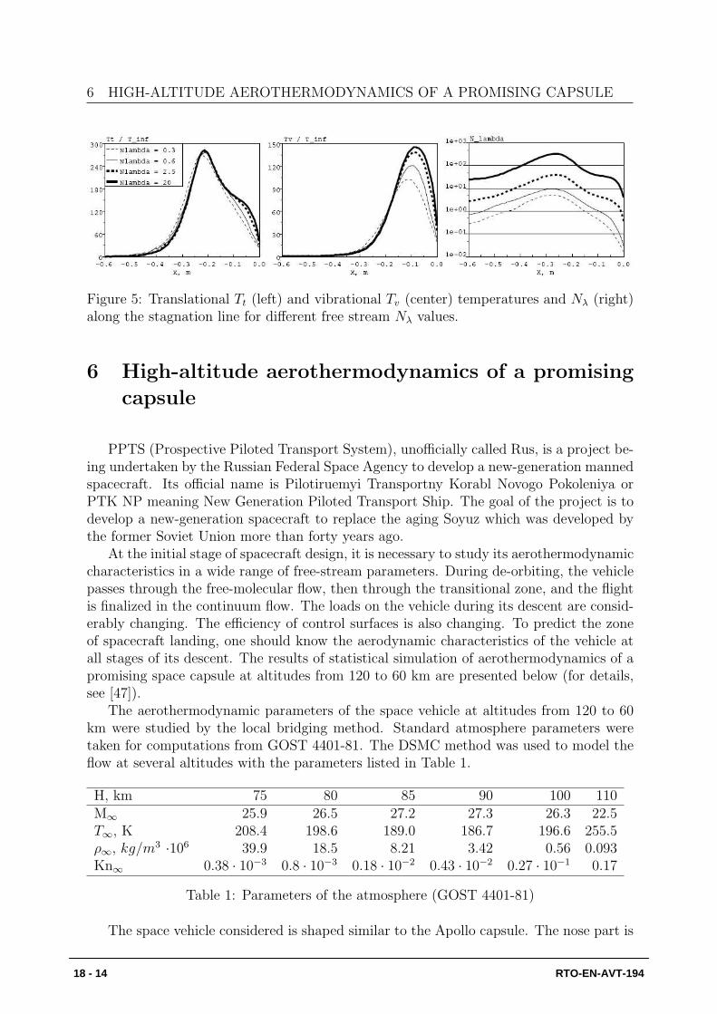
At the initial stage of spacecraft design, it is necessary to study its aerothermodynamiccharacteristics in a wide range of free-stream parameters. During de-orbiting, the vehiclepasses through the free-molecular flow, then through the transitional zone, and the flightis finalized in the continuum flow. The loads on the vehicle during its descent are consid-erably changing. The efficiency of control surfaces is also changing. To predict the zoneof spacecraft landing, one should know the aerodynamic characteristics of the vehicle atall stages of its descent. The results of statistical simulation of aerothermodynamics of apromising space capsule at altitudes from 120 to 60 km are presented below (for details,see [47]).

The aerothermodynamic parameters of the space vehicle at altitudes from 120 to 60km were studied by the local bridging method. Standard atmosphere parameters weretaken for computations from GOST 4401-81. The DSMC method was used to model theflow at several altitudes with the parameters listed in Table 1.

H, km 75 80 85 90 100 110M∞ 25.9 26.5 27.2 27.3 26.3 22.5T∞, K 208.4 198.6 189.0 186.7 196.6 255.5ρ∞, kg/m3 ·106 39.9 18.5 8.21 3.42 0.56 0.093Kn∞ 0.38 · 10−3 0.8 · 10−3 0.18 · 10−2 0.43 · 10−2 0.27 · 10−1 0.17

Table 1: Parameters of the atmosphere (GOST 4401-81)

The space vehicle considered is shaped similar to the Apollo capsule. The nose part is

18 - 14 RTO-EN-AVT-194


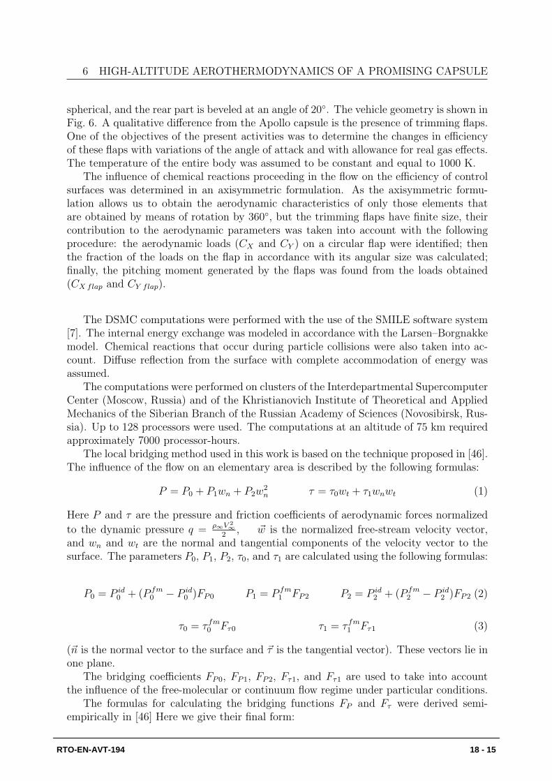
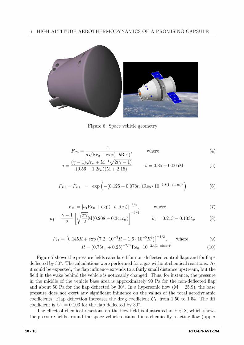
spherical, and the rear part is beveled at an angle of 20◦. The vehicle geometry is shown inFig. 6. A qualitative difference from the Apollo capsule is the presence of trimming flaps.One of the objectives of the present activities was to determine the changes in efficiencyof these flaps with variations of the angle of attack and with allowance for real gas effects.The temperature of the entire body was assumed to be constant and equal to 1000 K.

The influence of chemical reactions proceeding in the flow on the efficiency of controlsurfaces was determined in an axisymmetric formulation. As the axisymmetric formu-lation allows us to obtain the aerodynamic characteristics of only those elements thatare obtained by means of rotation by 360◦, but the trimming flaps have finite size, theircontribution to the aerodynamic parameters was taken into account with the followingprocedure: the aerodynamic loads (CX and CY ) on a circular flap were identified; thenthe fraction of the loads on the flap in accordance with its angular size was calculated;finally, the pitching moment generated by the flaps was found from the loads obtained(CX flap and CY flap).

The DSMC computations were performed with the use of the SMILE software system[7]. The internal energy exchange was modeled in accordance with the Larsen–Borgnakkemodel. Chemical reactions that occur during particle collisions were also taken into ac-count. Diffuse reflection from the surface with complete accommodation of energy wasassumed.

The computations were performed on clusters of the Interdepartmental SupercomputerCenter (Moscow, Russia) and of the Khristianovich Institute of Theoretical and AppliedMechanics of the Siberian Branch of the Russian Academy of Sciences (Novosibirsk, Rus-sia). Up to 128 processors were used. The computations at an altitude of 75 km requiredapproximately 7000 processor-hours.

The local bridging method used in this work is based on the technique proposed in [46].The influence of the flow on an elementary area is described by the following formulas:

P = P0 + P1wn + P2w2n τ = τ0wt + τ1wnwt (1)

Here P and τ are the pressure and friction coefficients of aerodynamic forces normalized

to the dynamic pressure q = ρ∞V 2∞

2, ~w is the normalized free-stream velocity vector,

and wn and wt are the normal and tangential components of the velocity vector to thesurface. The parameters P0, P1, P2, τ0, and τ1 are calculated using the following formulas:

P0 = P id0 + (P fm

0 − P id0 )FP0 P1 = P fm

1 FP2 P2 = P id2 + (P fm

2 − P id2 )FP2 (2)

τ0 = τ fm0 Fτ0 τ1 = τ fm1 Fτ1 (3)

(~n is the normal vector to the surface and ~τ is the tangential vector). These vectors lie inone plane.

The bridging coefficients FP0, FP1, FP2, Fτ1, and Fτ1 are used to take into accountthe influence of the free-molecular or continuum flow regime under particular conditions.

The formulas for calculating the bridging functions FP and Fτ were derived semi-empirically in [46] Here we give their final form:

RTO-EN-AVT-194 18 - 15


Figure 6: Space vehicle geometry

FP0 =1

a√Re0 + exp(−bRe0)

, where (4)

a =(γ − 1)

√tw +M−1

√

2(γ − 1)

(0.56 + 1.2tw)(M + 2.15)b = 0.35 + 0.005M (5)

FP1 = FP2 = exp(

−(0.125 + 0.078tw)Re0 · 10−1.8(1−sinαl)2

)

(6)

Fτ0 = [a1Re0 + exp(−b1Re0)]−3/4 , where (7)

a1 =γ − 1

2

[√

πγ

2M(0.208 + 0.341tw)

]−3/4

b1 = 0.213− 0.133tw (8)

Fτ1 =[

0.145R + exp(

7.2 · 10−3R− 1.6 · 10−5R2)]−1/2

, where (9)

R = (0.75tw + 0.25)−2/3 Re0 · 10−2.4(1−sinαl)3

(10)

Figure 7 shows the pressure fields calculated for non-deflected control flaps and for flapsdeflected by 30◦. The calculations were performed for a gas without chemical reactions. Asit could be expected, the flap influence extends to a fairly small distance upstream, but thefield in the wake behind the vehicle is noticeably changed. Thus, for instance, the pressurein the middle of the vehicle base area is approximately 90 Pa for the non-deflected flapand about 50 Pa for the flap deflected by 30◦. In a hypersonic flow (M = 25.9), the basepressure does not exert any significant influence on the values of the total aerodynamiccoefficients. Flap deflection increases the drag coefficient CD from 1.50 to 1.54. The liftcoefficient is CL = 0.103 for the flap deflected by 30◦.

The effect of chemical reactions on the flow field is illustrated in Fig. 8, which showsthe pressure fields around the space vehicle obtained in a chemically reacting flow (upper

18 - 16 RTO-EN-AVT-194


P, Pa

3.254e+006.779e+001.061e+011.479e+011.937e+012.440e+012.997e+013.616e+014.307e+015.084e+015.966e+016.973e+018.135e+019.491e+011.109e+021.302e+021.537e+021.830e+022.208e+022.712e+023.417e+024.474e+026.237e+029.762e+02

Figure 7: Pressure fields. Altitude 75 km. Chemically inert gas. Non-deflected flap(upper) and flap deflected by 30◦(downer).

figure) and in a chemically inert gas (lower figure) for the flap deflected by 30◦. Thecalculations were performed for an altitude of 75 km. It is seen that the flow fields aredrastically different in the entire computational domain. Indeed, as the major part of thefree-stream energy is spent on dissociation of diatomic molecules, the flow temperature inthe case of a chemically reacting gas is substantially lower than the temperature obtainedwith the chemical reactions being ignored. In addition to temperature fields, the Machnumber fields are also essentially different. Therefore, we can conclude that the entireflow structure and the shock waves near the vehicle are formed in a different manner.

P, Pa

3.246e+006.762e+001.058e+011.475e+011.932e+012.434e+012.989e+013.606e+014.296e+015.071e+015.950e+016.955e+018.114e+019.467e+011.106e+021.298e+021.533e+021.826e+022.202e+022.705e+023.408e+024.463e+026.221e+029.737e+02

Figure 8: Pressure fields. Altitude 75 km. Flap deflection angle 30◦. Chemically reactinggas (upper figure) and chemically inert gas (lower figure).

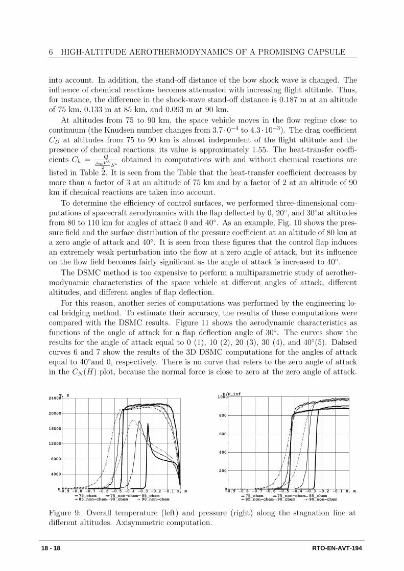
Figure 9 shows the distributions of temperature and pressure normalized to the free-stream pressure over the stagnation lines at altitudes of 75, 85, and 90 km. The plotsshow the stagnation lines obtained for chemically reacting and chemically inert gases.The plots on the left show the free-stream parameters, and the plots on the right showthe situation with the body located at X = 0. It is seen that the temperature of theflow behind the bow shock wave is substantially lower if chemical reactions are taken

RTO-EN-AVT-194 18 - 17


into account. In addition, the stand-off distance of the bow shock wave is changed. Theinfluence of chemical reactions becomes attenuated with increasing flight altitude. Thus,for instance, the difference in the shock-wave stand-off distance is 0.187 m at an altitudeof 75 km, 0.133 m at 85 km, and 0.093 m at 90 km.

At altitudes from 75 to 90 km, the space vehicle moves in the flow regime close tocontinuum (the Knudsen number changes from 3.7 ·0−4 to 4.3 ·10−3). The drag coefficientCD at altitudes from 75 to 90 km is almost independent of the flight altitude and thepresence of chemical reactions; its value is approximately 1.55. The heat-transfer coeffi-cients Ch = Q

ρ∞V 3

2S∗

obtained in computations with and without chemical reactions are

listed in Table 2. It is seen from the Table that the heat-transfer coefficient decreases bymore than a factor of 3 at an altitude of 75 km and by a factor of 2 at an altitude of 90km if chemical reactions are taken into account.

To determine the efficiency of control surfaces, we performed three-dimensional com-putations of spacecraft aerodynamics with the flap deflected by 0, 20◦, and 30◦at altitudesfrom 80 to 110 km for angles of attack 0 and 40◦. As an example, Fig. 10 shows the pres-sure field and the surface distribution of the pressure coefficient at an altitude of 80 km ata zero angle of attack and 40◦. It is seen from these figures that the control flap inducesan extremely weak perturbation into the flow at a zero angle of attack, but its influenceon the flow field becomes fairly significant as the angle of attack is increased to 40◦.

The DSMC method is too expensive to perform a multiparametric study of aerother-modynamic characteristics of the space vehicle at different angles of attack, differentaltitudes, and different angles of flap deflection.

For this reason, another series of computations was performed by the engineering lo-cal bridging method. To estimate their accuracy, the results of these computations werecompared with the DSMC results. Figure 11 shows the aerodynamic characteristics asfunctions of the angle of attack for a flap deflection angle of 30◦. The curves show theresults for the angle of attack equal to 0 (1), 10 (2), 20 (3), 30 (4), and 40◦(5). Dahsedcurves 6 and 7 show the results of the 3D DSMC computations for the angles of attackequal to 40◦and 0, respectively. There is no curve that refers to the zero angle of attackin the CN(H) plot, because the normal force is close to zero at the zero angle of attack.

-0.9 -0.8 -0.7 -0.6 -0.5 -0.4 -0.3 -0.2 -0.1 X, m0

4000

8000

12000

16000

20000

24000 T, K

75_chem 75_non-chem 85_chem85_non-chem 90_chem 90_non-chem

-0.9 -0.8 -0.7 -0.6 -0.5 -0.4 -0.3 -0.2 -0.1 X, m0

200

400

600

800

1000 P/P_inf

75_chem 75_non-chem 85_chem85_non-chem 90_chem 90_non-chem

Figure 9: Overall temperature (left) and pressure (right) along the stagnation line atdifferent altitudes. Axisymmetric computation.

18 - 18 RTO-EN-AVT-194


Altitude, km 75 80 85 90Chemically reacting flow 1.30 · 10−2 2.11 · 10−2 3.38 · 10−2 6.18 · 10−2

Chemically inert flow 4.30 · 10−2 6.22 · 10−2 9.47 · 10−2 1.36 · 10−1

Table 2: Heat-transfer coefficient Ch of the vehicle. DSMC results. Non-deflected flaps.Axisymmetric model

Figure 10: Pressure field and surface distribution of the pressure coefficient. Altitude 80km. Flap deflection angle 30◦. Angle of attack: 0 (left) and 40◦(right)

The moment characteristic differs from zero, because the center of gravity is shifted downon 0.156 m from the spacecraft axis. The curves obtained by the engineering methoddescribe the aerodynamic coefficients in the range of altitudes between 120 and 60 km.The difference from the DSMC results is approximately 5% for the force characteristics.The accuracy of the moment characteristics is lower, especially at an angle of attack of40◦at altitudes of 100 and 110 km (about 50%). It should be mentioned, however, that thevalue of the pitching moment coefficient is close to zero, and the large relative differenceactually means insignificant absolute difference in the pitching moment coefficient. TheDSMC computations reveal a significant effect of chemical reactions on the flow fieldsaround the spacecraft and on the heat-transfer coefficient at altitudes below 90 km. Be-cause of considerable changes in the flow structure near the base surface of the spacecraft,

60 70 80 90 100 110 H, km0.8

1.0

1.2

1.4

1.6

1.8

2.0

2.2CA

1 2 3 4 5 6 7

60 70 80 90 100 110 H, km0.0

0.2

0.4

0.6

0.8

1.0

1.2CN

1 2 3 4 5 6

60 70 80 90 100 110 H, km-0.08

-0.04

0.00

0.04

0.08

0.12

0.16Cm

1 2 3 4 5 6 7

Figure 11: Axial and normal force coefficients and pitching moment coefficient versusaltitude for different angles of attack. Flap deflection angle 30◦. Angle of attack 0◦(1),10◦(2), 20◦(3), 30◦(4), and 40◦(5); DSMC results for the angle of attack equal to 40◦(6)and 0◦(7).

RTO-EN-AVT-194 18 - 19

8 ACKNOWLEDGMENTS

there is a several-fold difference in the values of the pitching moment and the lift force ofthe vehicle with deflected control surfaces, which were obtained with and without chem-ical reactions. Simultaneously, chemical reactions proceeding in the gas exert practicallyno effect on the drag coefficient. The changes in the aerodynamic characteristics withvariations of the angle of attack and the angle of flap deflection at altitudes from 80 to110 km were computed by the DSMC method. The aerodynamic characteristics of thespacecraft at altitudes from 120 to 60 km were also calculated by the engineering localbridging method. Comparisons with the DSMC results showed that the axial and normalforce coefficients are calculated rather accurately (within 5%). The results obtained canbe used to design the thermal protection system of the space vehicle and to construct itsde-orbiting trajectory.

7 Prospects for the DSMC method

In conclusion, let us mention the directions for the DSMC method development thatwe believe will be important in the next several years.

• near-continuum flows: modeling of flows at relatively high Reynolds numbers (20,000and higher) using both conventional DSMC method and computationally efficienthybrid approaches

• real gas effects: development of general models applicable for any type of moleculesthat would accurately predict the energy transfer processes and chemical reactions

• numerical accuracy check: use of available and development of new criteria thatenable one to evaluate the numerical accuracy of results obtained, especially in thenear-continuum regime

• extensive validation of models and algorithms: comparison of DSMC results withexperimental data and continuum results in different gas dynamic situations forinert and reacting gases

• efficient parallel algorithms with dynamic load balancing: these are critical for mod-eling of computationally intensive two- and three-dimensional problems

8 Acknowledgments

The author would like to thank the research team of the Computational AerodynamicsLaboratory of the Institute of Theoretical and Applied Mechanics, Siberian Branch ofthe Russian Academy of Sciences. Our special thanks to Yevgeniy Bondar, AlexanderKashkovsky, Dmitry Khotyanovsky, Alexei Kudryavtsev, Gennady Markelov, AlexanderShevyrin, Alina Alexeenko and Pavel Vashchenkov, who provided results of computationsand participated in discussions and preparation of this paper. This work was supportedby the Russian Foundation for Basic Research (Grant No. 10-08-01203-a).

18 - 20 RTO-EN-AVT-194

A APPENDIX 1. MAJORANT COLLISION FREQUENCY SCHEMES

A Appendix 1. Majorant collision frequency schemes

The DSMC method is traditionally considered as a method of statistical simulation ofthe behavior of a great number of model gas molecules. Usually the number of simulatedparticles is large enough (∼ 105−108), but this is extremely small in comparison with thenumber of molecules that would be present in the real gas flow. Each simulated particleis then regarded as representing an appropriate number of real molecules.

The state of each simulated particle is characterized by its coordinate r and velocity v.The state of the whole system of N particles is described by the 6N -dimensional vector{R, V } = {r1, v1, ..., rN , vN}. The evolution of such a system can be represented as ajump-like motion of a point in the 6N -dimensional phase space. The DSMC method canbe then treated as statistical simulation of the 6N -dimensional random jump-like process.For such a simulation, it is necessary to generate the trajectory of the random process.To this end, it is needed to determine a technique for simulation of the initial trajectorypoint of the random process (t0, R0, V0), transition in time between subsequent collisions(free motion) from the state (t0, R0, V0) to the state (t1, R1, V0), and the changes in particlevelocities after collisions, i.e. the transition from the state (t1, R1, V0) to (t1, R1, V1). Thentransitions from state 1 to state 2, etc. are considered. The trajectory is terminated whentn > T where T is the modeling time.

In the traditional approach of constructing numerical schemes of the DSMC method[1], the description of procedures for trajectory simulation of the random process is basedon physical concepts of rarefied gas and on physical assumptions that form the basis forthe phenomenological derivation of the Boltzmann equation.

The kinetic theory of gases makes use of the so-called“master”kinetic equations (MKE)[3,4] which describe the behavior of an N -particle gas model with binary collisions. Theselinear MKE transform to the nonlinear Boltzmann equation when N → ∞ and molecularchaos conditions are satisfied (see, e.g., [5] ). Since a finite number of simulated particlesis used in numerical simulation, it is natural to utilize directly these MKE equations forconstructing numerical schemes of the DSMC method. Such an approach to the derivationof numerical schemes of the DSMC method was presented in [2,33,37].

First, let us consider a spatially-uniform rarefied gas flow, and present the main stepsof constructing numerical schemes directly from the MKE. In this case, it is possible touse the Kac master equation [3]:

∂

∂tfN(t, V ) =

n

N

∑

i<j

∫ 2π

0

dǫij

∫ ∞

0

bijdbij|vi − vj|{fN(t, V ′ij)− fN(t, V )}, (1)

where V = (v1, . . . , vN) is a 3N -dimensional vector of particle velocities; V ′ij = (v1, . . . ,

v′i, . . . , v′j , . . . , vN); bij and ǫij are the impact parameters; (v′i, v

′j) and (vi, vj) are the pre-

and post-collisional velocities of i, j molecules, n is the number density, and the sum overi < j means the summation over N(N − 1)/2 collision pairs.

This is a linear integro-differential equation that describes the time behavior of theN -particle distribution function fN(t, V ),

∫

fN(t, V )dV = 1.In accordance with the general theory of Monte Carlo methods [39,40], the following

approach is used: the transition from an integro-differential form of the master kinetic

RTO-EN-AVT-194 18 - 21


equation to a linear integral equation whose probability treatment serves as the basis forconstructing an appropriate random process of direct simulation.

Using a function w – the probability density of transition of a pair of particles from(v′i, v

′j) to (vi, vj), eqn (1) is written as

∂

∂tfN(t, V ) + ν(V )fN(t, V ) =

n

N

∑

i<j

∫

fN(t, V′ij)w(v

′i, v

′j → vi, vj)dv

′idv

′j, (2)

where ν(V ) is the total collision frequency

ν(V ) =n

N

∑

i<j

∫

w(v′iv′j → vi, vj)dv

′idv

′j =

n

N

N∑

l=j

∫

σ (gij, ξij) δ3(

vi + vj − v′i − v′j)

×

×δ1(

(vi − vj)2 −

(

v′i − v′j)2

2

)

dv′idv′j =

n

N

∑

i<j

σt(gij)gij <∞ (3)

and g is the relative collision velocity, σt(gij) and σ(gij, ξij) are the total and differentialcollision cross-sections, and χij is the deflection angle.

The total collision frequency (3) determines the time of the next collision in the systemand depends on velocities of all particles, and it is necessary to recalculate its value aftereach collision. This is rather time-consuming if the number of particles N is large, sincethe summation is performed over all possible N(N − 1)/2 collision pairs.

Let us introduce the majorant collision frequency [33]

νm =N(N − 1)

2[gσt(g)]max ≥ ν(V ). (4)

Then we add to the both sides of eqn (2) the corresponding sides of the equality

[νm − ν(V )]fN(t, V ) =n

N

∑

i<j

∫

fN(t, V′){

[gσt(g)]max − g′ijσt(g′ij)}

δ(V − V ′)dV ′

and join the right-side integrals to have

∂

∂tfN(t, V ) + νmfN(t, V ) =

=n

N

∑

i<j

∫

fN(t, V′)

{

[

[gσt(g)]max − g′ijσt(g′ij)]

δ(vi−v′i)δ(vj−v′j)+w(v′i, v′j → vi, vj)

}

dv′idv′j.

(5)Here δ denotes Dirac’s delta-function.

Let us introduce the function ψ(t, V ) as

fN(t, V )ν(V ) =

∫ ∞

0

K2(t′ → t|V )ψ(t′, V )dt′,

where K2 is the kernel

K2(t′ → t|V ) = θ(t− t′)ν(V ) exp

{

−ν(V )(t− t′)}

18 - 22 RTO-EN-AVT-194


and θ is the Heaviside function, then eqn (5) may be transformed to an integral form

ψ(t, V ) =

∫ ∞

0

∫

K21ψ(t′, V ′)dV ′dt′ + δ(t)f 0

N(V ) (6)

with the kernelK21 = K2(t

′ → t|V ′)K1(V′ → V ).

HereK2(t

′ → t|V ′) = θ(t− t′)νm exp{−νm(t− t′)},

K1(V′ → V ) =

∑

i<j

2

N(N − 1)×

×{

[

1−g′ijσt(g

′ij)

[gσt(g)]max

]

δ(vi− v′i)δ(vj− v′j)+g′ijσt(g

′ij)

[gσt(g)]max

w(v′i, v′j → vi, vj)

g′ijσt(g′ij)

}

N∏

m=1

m 6=i,j

δ(vm− v′m).

The probability treatment of eqn (6) enables one to construct a random process thatdescribes the behavior of the N -particle gas model. To calculate the initial trajectorypoint of this process, the free term from eqn (6) is used as the probability density, whilethe kernel K21 yields the probability density of the transition from

the state (t′, V ′) to the state (t, V ).

This transition is modeled sequentially from

the state (t′, V ′) to (t, V ′)

in accordance with the distribution density K2(t′ → t|V ′).

Then, in compliance with the kernel K1(V′ → V ) the transition (t, V ′) → (t, V ) occurs.

For this purpose, a collisional pair (i, j) is uniformly chosen from N(N − 1)/2 pairs(this is evidenced by the presence of the factor 2/N(N − 1) in the kernel K1). A collisionof this pair occurs with the probability

P =g′ijσt(g

′ij)

[gσt(g)]max,

and with the probability (1 − P ) the velocities will not change (this is evidenced by thepresence of the product of two delta-functions in the first term of the kernel K1), i.e. afictitious collision occurs. The product of delta-functions inK1 (the last factor) shows thatafter a collision of the pair (i, j) velocities of other particles remain unchanged, whereasvelocities (v′i, v

′j) for real collisions are replaced by post-collisional velocities (vi, vj).

Collision impact parameters are selected with the probability

w(v′i, v′j → vi, vj)

g′ijσt(g′ij)

,

and the presence of two delta-functions δ3 and δ1 in w (see (3)) shows that new velocitiesare calculated in accordance with momentum and energy conservation laws.

RTO-EN-AVT-194 18 - 23


Thus, all required procedures for trajectory simulation of the random process arespecified, and the numerical scheme of the DSMC method is constructed for a spatiallyuniform case. Its computer cost is proportional to the number of simulated particles [2].

Usually in problems of rarefied gas dynamics it is required to determine gas parametersat the time moment tk, which have the form

Ih(tk) =

∫

h(v)f1(tkv)dv =

∫

H(V )fNdV ,

where h(v) is the function of velocity, and

H =1

N

∑

h(v).

To calculate functionals, such as Ih(tk), it is possible to use the estimates knownfrom the general theory of Monte-Carlo methods [40]. In particular, a counterpart of thenon-biased absorption estimate has the form

ξψ = H(Vs), s = max{n : tn < ti, n = 0, 1, ...}.

Approximate values Ih(tk) of the functionals Ih(tk) are given by

Ih(tk) = L−1

L∑

l=1

ξψ(l),

where L is the number of independent N -particle trajectories of a random process. Fol-lowing [33], it can be shown that the mathematical expectation is

E[ξψ] = Ih(tk),

and the variance of random variable ξψ is

V ar [ξΨ] = N−1

{∫

h2 (v) f1 (t, v) dv − I2h (tk)

}

+

+N − 1

N

∫

h (v1)h (v2) {f2 (t, v1, v2)− f1 (t, v1) f (t, v2)} dv1dv2. (7)

It is known [39] that the variance of absorption estimate is limited and, by the centrallimit theorem, the following inequality is valid:

∣

∣

∣

∣

∣

L−1

L∑

l=1

ξlΨ − Ih (tk)

∣

∣

∣

∣

∣

≤ 3

√

V ar [ξΨ]

L

It is commonly believed that the statistical error of the DSMC method is determinedonly by the overall volume of the sampling, (N · L). It follows from (7) that under thecondition of molecular chaos (f2 = f1f1) the second term vanishes, and the statisticalerror is proportional to

1/√N · L.

18 - 24 RTO-EN-AVT-194


For finite N , however, there is always a statistical dependence of particles (see [33] formore detail); and, hence, the statistical error is proportional to

1/√L.

To analyze the relationship between simulation results and the solution of the Boltz-mann equation, it is necessary to consider the kinetic equation for the one-particle distri-bution function

f1(t, v1) =

∫

fN(t, VN)dv2...dvN .

If Kac MKE equation (1) is integrated over (N−1) variables v2, ..., vN , then we obtaina kinetic equation for the one-particle distribution function

∂

∂tf1 =

N − 1

Nn

∫ 2π

0

dǫ

∫ ∞

0

b db×

×∫

dv2|v1 − v2|(f1(v′1)f1(v′2)− f1(v1)f1(v2))+

+N − 1

Nn

∫ 2π

0

dǫ

∫ ∞

0

b db

∫

dv2|v1 − v2|(g′2 − g2), (8)

where g2 = f2 − f1f1. In the general case the solution of equation (8) differs consider-ably from the solution of the Boltzmann equation, since it depends on the variation ofthe two-particle correlation function g2(t, v1, v2). Examples of the influence of statisticaldependence of particles on the simulation results were presented in [33]. Equation (8) istransformed into the Boltzmann equation [41] when N → ∞ and the molecular chaoshypothesis is valid. Strictly speaking, only under these conditions the results of statisticalsimulation precisely correspond to the solution of the Boltzmann equation.

It is shown therefore, that the use of the MKE allows one to obtain not only a prob-abilistic procedure for simulation of the random process and statistical estimates for cal-culating the gas parameters, but also to assess the statistical error of results. In addition,the relationship between the results of simulation of the N -particle gas model and thesolution of the Boltzmann equation has become more transparent.

The next step is to illustrate how the approach described can be extended to a spa-tially nonuniform case. The traditional approach [1] employs the discretization of spatial-temporal evolution of the N -particle gas model. A continuous process of motion andcollisions of molecules is uncoupled, the computational domain is divided into cells, andthe following processes are sequentially simulated at each step ∆t:

• spatially uniform relaxation of the gas in each cell;

• free-molecular movement of simulated particles over the distances appropriate to ∆twith regard for boundary conditions.

A different approach was proposed by Ivanov and Rogasinsky [2] who constructednumerical schemes for simulating a 6N -particle, continuous in time, random process of

RTO-EN-AVT-194 18 - 25


spatially nonuniform evolution of a system of N particles. These schemes were deriveddirectly from the Leontovich master kinetic equation [4]:

∂fN∂t

+N∑

i=1

vi∂fN∂ri

fN =∑

i<j

δ(ri − rj)

∫

{f ′N − fN}|vi − vj|bijdbijdǫij. (9)

Here fN = fn(t, R, V ), f ′N = fn(t, R, V

′ij) are the N -particle distribution functions, and

∫

fNdV dR = 1.

The relationship between this equation and spatially nonuniform Boltzmann equationwas studied in [5].

The presence of the delta-function in collision integral (9) indicates the collision “lo-cality”, i.e. identical coordinates of colliding particles, like in the Boltzmann equation.For numerical simulation one has to perform the regularization of collision integral (9),i.e. introduce “smeared”particle interactions. Using the function wρ, the collision integralin eqn (9) takes the form

JN =N∑

i=j

∫

(

f′

N − fN

)

wρdv′

idv′

j,

wherewρ

(

v′

i, v′

j → vi, vj|ri, rj, ρ)

is the probability density of transition of the pair (i, j) from the state (v′i, v′j) to the state

(vi, vj) with fixed values of particle coordinates (ri, rj) and regularization parameter ρ. Inthis case,

wρ

(

v′

i, v′

j → vi, vj|ri, rj, ρ)

→ δ (ri − rj)w(

v′

i, v′

j → vi, vj

)

when ρ→ 0

Let us consider the following regularization

wρ

(

v′

i, v′

j → vi, vj|ri, rj , ρ)

= h(ri, rj)w(

v′

i, v′

j → vi, vj

)

,

h(ri, rj) =

{

ω−10 , if |ri − rj| < ρ,0, if |ri − rj| > ρ,

ω0 =4

3π ρ3.

The parameter ρ defines the dimension of the “interaction region” of particles, and itsvalue depends on the required accuracy of calculation of flow parameters.

Then, the total collision frequency of an N -particle gas model is as follows

νρ(R, V ) =N∑

i<j

h(ri, rj)gijσt(gij) <∞, (10)

18 - 26 RTO-EN-AVT-194


and it depends on the particle coordinates and velocities. As in the case of a uniformgas model, the calculation of this collision frequency requires the summation of N(N −1)/2 pairs with checking the distance between the particles, which is time-consuming.Therefore, here it is again profitable to majorize the collision frequency, and contrary to(4) not only with respect to the particle velocities, but also to the coordinates of collidingparticles.

Let us choose the majorant collision frequency in the form

νm =N(N − 1)

2ω−10 [gσt(g)]max ≥ ν(R, V ), (11)

and transform the Leontovich equation, similar to the uniform case, to the following form:

∂fN∂t

+N∑

i=1

vi∂fN∂ri

fN + νmfN =

=N∑

i<j

∫

f ′N

{

h(ri, rj)ω−10 w(v′i, v

′j → vi, vj)+

+(

[gσt(g)]maxω−10 − h(ri, rj)ω

−10 gijσt(gij)

)

× δ(v′i − v′i)δ(v′j − v′j)

}

dv′idvj. (12)

The collision integral here consists of two parts corresponding to real (first term) andfictitious (second term) collisions.

The use of such a majorant collision frequency νm allows one, therefore, to trans-form the nonuniform problem under consideration to a spatially uniform problem with aconstant collision frequency.

If eqn (12) with appropriate initial and boundary conditions is transformed to a linearintegral equations (see details in [2]), then the probability treatment of the kernel and freeterm of this equation allows for formulating a new scheme of direct statistical simulationof spatially nonuniform rarefied gas flow with continuous time.

Below, the salient points in simulation of a 6N -dimensional trajectory of the randomprocess of the transition of an N -particle system from the state (t′, R′, V ′) to (t, R, V ) arebriefly described.

We shall not dwell here upon the simulation of particles entering the computationaldomain and the interaction of particles with the body surface. All details can be foundin [2].

The time of the next collision t has the probability density distribution

νm exp {−νm(t− t′)} ,

while the probability density of the transition of a system of N particles from the state(t′, R′, V ′) to (t, R, V ′) is the delta-function

δ(R− R′ − V ′(t− t′)).

This means that all simulated particles move during the time t − t′ from point R′ to Rwith velocities V ′.

RTO-EN-AVT-194 18 - 27


An examination whether the collision is real is performed as follows:if |ri− rj| > ρ then the collision is fictitious, else the collision is real with the probability

gijσt(gij)

[gσt(g)]max

and fictitious with the complementary probability.Thus, all probabilistic procedures necessary for the numerical generation of the tra-

jectories of a 6N -dimensional random process of evolution of a spatially nonuniform N -particle gas model are described.

For regularization of the collision integral in eqn (9) it is also possible to use a usualapproach of the DSMCmethod: the computational domain is divided into non-intersectingcells dk, so that

M∑

k=1

dk = V0,

and a collision may occur only between particles that belong to the same cell. Then themajorant collision frequency has the form

νm =N(N − 1)

2[gσt(g)]maxd

−1min, dmin = min(dk). (13)

A collision of the pair (i, j) randomly chosen from all N(N − 1)/2 pairs is fictitious if theparticles i and j are in different cells.

The use of the majorant collision principle for spatially nonuniform case with theregularization of the type (11) or (13) allows one, therefore, to obtain a new exact time-continuous scheme of the DSMC method.

A salient point that differs this scheme from the conventional DSMC method is thetransfer of all particles after each collision. Certainly, this is extremely expensive; there-fore, only examples of using this algorithm for 1D rarefied gas dynamic problems (shockwave structure and Couette flow) are now available. However, the mere fact that it ispossible to simulate rarefied gas flows, avoiding uncoupling of a continuous process ofmolecular motion and collisions, is of principal importance. Possibly, this approach canbe used in future when the computer performance significantly increases.

It is natural to consider an approximate simulation scheme with separated and se-quentially calculated collisions and motions of particles.

Let us introduce discrete time instants tn = n ·∆t and choose a step ∆t such that foreach τm, provided

∑

m τm ≤ ∆t, the following condition is valid:

νρ(

R + τm · V , V |ρ)

≈ νρ(

R, V |ρ)

This means that the change in collision probability of pairs due to particle displacementis ignored during the time ∆t. Then an approximate simulation scheme is as follows: thetime between consecutive collisions is chosen on the basis of the probability density

νm exp {−νm(τ)} .

If∑

τ lm < ∆t,

18 - 28 RTO-EN-AVT-194


then a collision (real or fictitious) occurs. All particles are displaced at a distance pro-portional to ∆t one time, at the end of the step ∆t.

Numerical schemes with a continuous and discrete time that make use of the majorantcollision frequency with the regularization of types (11) or (13) do not employ the sortingof particles over cells and, therefore, can be called free cell schemes. The determinationof distributed and total aerodynamic characteristics can be conducted directly using onlythe collisions of a particle with the body surface. The calculation of flowfields requires agrid for sampling the gas parameters, but this grid is not related to collision simulation.

The value of the free cell majorant can be reduced by sorting the particles over thecells. Then

νm =M∑

k=1

νkm =M∑

k=1

Nk(Nk − 1)

2

[gσt(g)]kmax

dk, (14)

where Nk is the number of molecules in the k-th cell. Obviously,

νcellm < νfreecellm

and, hence, the computational cost of the cell scheme is smaller than that of the free cellscheme. In the cell scheme, however, it is necessary to take into account the cost of particlesorting over cells. This sorting is very simple in the case of a rectangular Cartesian grid,but with using more complex adaptive body-fitted grids its cost drastically increases.

When using the cell regularization with the majorant (14), having determined the timeof the next collision τ lm at the step ∆t, one has to determine the number of the cell inwhich this collision occurs. The cell number, k, is selected with the probability νkm/νm.Then a pair (i, j) is uniformly chosen in the k-th cell from Nk particles. The collision isreal with the probability

gijσt(gij)

[gσt(g)]max

and fictitious with the complementary probability.The mean number of collisions in a system of N particles during the time ∆t is νm∆t,

and each cell is chosen with the probability νkm/νm. Consequently, during the time ∆teach cell is chosen νkm∆t times in the average. Then for νkm∆t ≫ 1 there is no need tosample the cell number, and the usual sequential computation of collisions over all cellscan be employed.

The scheme that uses the cell regularization with particle sorting and probabilisticchoice of the cell number where a collision will occur can be called a cell majorant collisionfrequency scheme.

Our experience of using the cell and free cell schemes, which has been accumulatedup to now, shows that these schemes should not be set in opposition. Vice versa, it isdesirable to use them together. For this purpose, the computational domain is dividedinto uniform Cartesian cells with the linear dimension of the order of λ∞, and the cellscheme is used there. In flow areas where the local mean free path strongly decreases andin the vicinity of the body surface, the free cell scheme is used with a small regularizationparameter in order to increase the spatial collision resolution.

Now a few words about the influence of the finite number of simulated particles onthe results of computations. In the nonuniform case, the main criterion that allows fora practical verification of the presence of a statistical dependence between the simulated

RTO-EN-AVT-194 18 - 29


particles is the relative number of repeated collisions. Here, repeated collisions are colli-sions between the same pair of particles during their lifetime in the computational domain.This number is directly related to the number of particles Nλ in a volume with linear sizeof the local mean free path. If Nλ ≥ 1, we can definitely say that the simulation resultsare close to the solution of the Boltzmann equation.

This is certainly only an intuitive, experience-based criterion. A more detailed studyof the influence of statistical dependence with the use of autocorrelation functions andthe number of repeated collisions can be found in [42].

The extension of the majorant collision frequency schemes, directly obtained from theMKE, to the case of multi-species chemically reacting mixtures is straightforward. Itimplies the change in cross-sections of the corresponding inelastic processes and, hence,the change in the collisional algorithm only in its part that refers to collision mechanics.

18 - 30 RTO-EN-AVT-194

A APPENDIX 2. GAS/SURFACE INTERACTION MODELS

A Appendix 2. Gas/surface interaction models

Calculation of aerodynamic forces by the DSMC method requires setting the veloc-ity distribution functions for molecules reflected from the object surface. A simplifiedrepresentation of this function is used, which must take into account the major featuresof gas-surface interaction which have been revealed in experiments (force action, angu-lar distribution of molecules escaped), on the one side, and it must be simple enough inapplication, on the other side.

The main requirement of the surface properties definition is to introduce for everyelement of the space object the following surface properties:

1. Wall temperature

2. Scheme of gas-surface interaction (Maxwell or Nocilla) model, accommodation andinteraction coefficients.

If a space object consists of several hundred or thousand elements it is not convenientfor user to introduce or edit the properties of each element. So a procedure was found togive the user a fast possibility for introducing and editing with a maximum flexibility:

1. Setting surface properties for the geometric model. For each compound and elementa list of surface properties can be assigned.

2. Introducing and checking the surface properties of a compound. The system showsthe actual content of this compound and to each element surface properties can be as-signed.

3. To check the correct settings of the surface properties the system provides a visu-alization tool.

One of the oldest and most widely used distribution functions for the reflected moleculesis due to Maxwell [43].

It is constructed on the assumption that a fraction 1− σ of the molecules is reflectedfrom the surface in a specular fashion, while the fraction σ is re-emitted diffusely, withthe Maxwellian distribution:

fr(~r, ~ξr) = (1− σ) fi (~r, ~ξr − 2(~ξr · ~n)~n) + σ π−3/2 c′−3r exp

{

−~ξ2rc′2r

}

where ~ξr is the reflected velocity ~n is the external normal of the surface in point ~r, c′r isthe most probable speed at the temperature Tr.

The parameter σ is called the tangential momentum accommodation coefficient. Ev-idently, for completely specular reflection, σ = 0, while for complete diffuse reflection,σ = 1.

This implementation of the specular-diffuse scheme implies either specular or diffusereflection of particles. Therefore, at first, each particle is sampled to experience a par-ticular type of reflection. If the pseudo-random number is smaller than σ, the particleexperiences diffuse reflection; otherwise, it experiences specular reflection.

In the case of specular reflection, the velocity component normal to the surface changesits sign, and the tangential components of velocity remain unchanged.

RTO-EN-AVT-194 18 - 31


The velocity of diffusely reflected molecules is sampled in the local polar coordinatesystem, directed along the outer normal of the to surface of the vehicle, in the followingmanner:

| ~ξr |= c′r√

− ln(R1R2);

cos(ψ) =√

R3;

φ = 2π R4,

where | ~ξr | - module of the velocity of reflected particle; ψ, φ - polar and azimuthal anglesand R1, R2, R3, R4 are random numbers;

Following ref.[43] an energy accommodation coefficient σE = Ei−Er

Ei−Ewis used. When

the accommodation coefficient σE = 0 then the molecules don’t exchange energy with thewall, and σE = 1 if the incident molecules reached thermal equilibrium with the wall.

If we write the energy of a molecule in terms of its velocity, Eq. A takes the form:

σE =ξ2i − V 2

r

ξ2i − c′2r;

accordingly, the value of velocity with which the particles are reflected is written as

Vr =√

(1− σE)ξ2i + σEc′2r

Thus, for each diffusely reflected molecule, the absolute value of its sampled velocity| ~ξr | should be corrected by the coefficient

k =Vrc′r

=√

(1− σE)ξ2i /c′2r + σE,

and hence

| ~ξr |= kc′r√

− ln(R1R2).

The distribution function [44-45] for the velocities of reflected particles which is oftenused in practice has the following form:

fr = nr

(

1

π

m

2kTr

)3

2

exp

{

− m

2kTr

[

~ξ − ~Ur

]2}

=

= nr

(

1

π

m

2kTr

)3

2

exp

−[

(

m

2kTr

)1

2

~ξ − ~Sr

]2

=

= nr

(

1

π

m

2kTr

)3

2

exp

{

−[

(

m

2kTr

)1

2

ξy − Snr

]2

−[

(

m

2kTr

)1

2

ξx − Sτr,x

]2

−[

(

m

2kTr

)1

2

ξz − Sτr,z

]2}

Here m and ~ξ are the mass and velocity of molecules reflected from surface, andparameters of particle number density nr, temperature Tr and speed ~Ur depend on the

18 - 32 RTO-EN-AVT-194


velocity vector of a molecule incident upon the surface, as well as on its energy, surfacecharacteristics and total mass flow of incident molecules. These dependences transformto those of five scalar parameters of function fr on the base of available experimental dataand mass conservation law.

The experiments [44] showed that the vector of the mean reflected velocity is located inthe same plane as the vector of the incident velocity. Thus, if we construct the right-handCartesian coordinate system at the point of particle reflection so that the x axis is theprojection of the incident velocity vector onto a plane tangential to the surface, the y axiscoincides with the external normal to the surface, then the side component of reflectedvelocity is Sτr,z = 0.

The four parameters of this function Snr, Sτr,x, Tr, nr are found[44,45] as follows:

Snr = 0.1− 0.652θ

π,

Sτr,x =τr,xpr

· J2(Snr)J1(Snr)

,

2k

mTr =

(

prqmr

)2 [J1(Snr)

J2(Snr)

]2

,

nr = qmr

(

2k

mTr

)− 1

2

J−11 (Snr),

τr,x = −(

aτ + bτ4θ − π

2π

)

ξ sin(θ) qmi

pr =

{

(

an + bn2θ

π

)

ξ +

(

π

2

kTwm

)1

2

}

qmi

J1(t) =1√π

∫ ∞

0

q exp[

−(q − t)2]

dq =1√2π

[

e−t2

+√π t (1 + erf(t))

]

,

J2(t) =1√π

∫ ∞

0

q2 exp[

−(q − t)2]

dq =1√2π

[

te−t2

+√π (

1

2+ t2) (1 + erf(t))

]

,

erf(t) =2√π

∫ t

0

e−s2

ds,

qmr = qmi = mq1; q1 = 1[m−2 s−1].

Here θ is the angle between the incident velocity vector and internal normal to the surface,Tw is the surface temperature, qmr and qmi are the fluxes of reflected and incident molecules,which is used to normalize the distribution function fr in the Monte-Carlo method.

The values of model parameters an, bn, aτ , and bτ depend on the type of material, andthe following values were obtained [44,45] based on experimental data:

RTO-EN-AVT-194 18 - 33


Materials an bn aτ bτ

Ceramics 0.06 0.05 -0.03 0.26White enamel 0.07 0.10 -0.01 0.16Black enamel 0.065 0.08 -0.03 0.11Scree-vacuum glass Cloth 0.07 0.03 -0.05 0.11Anodized aluminium-magnesium Alloy (AMA) 0.10 0.10 -0.06 0.04Chemically polished AMA 0.11 0.18 -0.19 -0.04Glasses 0.17 0.09 -0.10 -0.08Enamels 0.07 0.06 -0.01 0.12

Sampling of velocity with which a particular particle is reflected involves the proba-bility density of reflected molecules, which is obtained from the distribution function andis written in the following form:

Fr,x =1√π√Trexp

{

−[

(

m

2kTr

)1

2

ξx − Sτr,x

]2}

Fr,y =2√

π√Tr J1(Snr)

(

m

2kTr

)1

2

ξy exp

{

−[

(

m

2kTr

)1

2

ξy − Snr

]2}

Fr,z =1√π√Trexp

{

−[

(

m

2kTr

)1

2

ξz

]2}

The velocity ξy is simulated by the Neumann method, and the velocities ξx and ξz aresimulated on the basis of the relations

ξxc′r

=√

− ln(R1) cos(2π R2) + Sτr, x

ξzc′r

=√

− ln(R1) sin(2π R2)

where R1 and R2 are pseudo-random numbers.

18 - 34 RTO-EN-AVT-194

REFERENCES REFERENCES

References

[1] Bird, G. A., Molecular gas dynamics and the direct simulation of gas flows, Clarendonpress, Oxford, 1994.

[2] Ivanov MS, Rogasinsky SV. 1991. Theoretical analysis of traditional and modernschemes of the DSMC method. Proc. 17th Int. Symp. on Rarefied Gas Dynamics,

Aachen, pp. 629-642, ed. AE Beylich, VCH

[3] Kac M. 1959. Probability and related topics in the physical sciences, Interscience, NewYork

[4] Leontovich, M. A., Soviet Physics JETP, 5, 211-231 (1935).

[5] Klimontovich, Yu. L., Uspehi Fiz. Nauk, 139, No. 4, 689-700 (In Russian) (1983).

[6] Koura, K., Phys. Fluids, 29, 3509-3511 (1986).

[7] Ivanov, M. S. , Markelov, G. N., Gimelshein, S. F., AIAA Paper 98-2669 (1998).

[8] Markelov, G. N., Ivanov, M. S., Journal of Spacecraft and Rockets, 38, No. 6, 875-881(2001).

[9] Ivanov, M.S., Markelov, G.N., Gimelshein, S.F. Mishina, L.V. Krylov, A.N, Greckho,N.V., 1998, ‘“High Altitude Capsule Aerodynamics with Real Gas Effects”, J. of Space-craft and Rockets, Vol.35. No. 1., pp.16-22.

[10] Haas, B. L., Boyd, I. D., AIAA Paper 91-0774 (1991).

[11] Koura, K., Phys. Fluids A, 4, No. 8, 1782-1788 (1992).

[12] Boyd, I. D., Phys. Fluids A, 5, No. 9, 2278-2286 (1993).

[13] Gimelshein, S. F., Gorbachev, Yu. E., Ivanov, M. S., Kashkovsky, A. V., Proc. of19 Int. Symp. on Rarefied Gas Dynamics, Oxford University Press, 1995, Vol. 1, pp.556-563.

[14] Boyd, I. D., Phys. Fluids A, 8, No. 5, 1293-1300 (1996).

[15] Koura, K., Matsumoto, H., Phys. Fluids A, 3, No. 10, 2459-2465 (1991).

[16] Gimelshein, S. F., Boyd, I. D., Ivanov, M. S., AIAA Paper 99-3451 (1999).

[17] Borgnakke, C., and Larsen, P. S., J. Comp. Phys., 18, No. 4, 1975, 405-420 (1975).

[18] Lumpkin, F. E., Haas, B. L., Boyd, I D., Phys. Fluids A, 3, No. 9, 2282-2284 (1991).

[19] Haas, B. L, Hash, D., Bird, G. A., Lumpkin, F. E., Hassan, H., Phys. Fluids A, 6,No. 6, 2191-2201 (1994).

[20] Gimelshein, S. F., Gimelshein, N. E., Levin, D. A., Ivanov, M. S., Markelov, G. N.,AIAA Paper 2002-2759 (2002).

RTO-EN-AVT-194 18 - 35


[21] Bergemann, F., Boyd, I. D., Rarefied Gas Dynamics: Theory and Simulations, 158,1994, edited by B. D. Shizgal and D. P. Weaver, Progress in Astronautics and Aero-nautics, 1994, pp. 174-183

[22] Choquet, I., Modelisation des desequilibres thermiques dans les ecoulements de gas

rarefies, Ph.D. thesis, L’universite Paris VI, (1993).

[23] Millikan, R. C., White, D. R., J. Chem. Phys., 39, No. 12, 3209-3213 (1996).

[24] Marriott, P. M., Non-equilibrium chemical reactions in the simulation of hypersonicrarefied flows, Ph.D. thesis, Imperial College of Science, Technology and Medicine,London, (1994).

[25] Gimelshein, S. F., Ivanov, M. S., Markelov, G. N., Gorbachev, Yu. E., “QuasiclassicalVRT transitional models in the DSMC computations of reacting flows”, Proc of the20 Int. Symp. on Rarefied Gas Dynamics, Beijing (1996).

[26] Koura, K., “Rotationally and vibrationally inelastic cross-section models for direct

simulation Monte Carlo methods”, Proc. of the 20 Int. Symp. on Rarefied Gas Dy-namics, Beijing (1996).

[27] Gimelshein, N. E., Gimelshein, S. F, Levin, D. A. “Vibrational relaxation rates inthe direct simulation Monte Carlo method”, Physics of Fluids.

[28] Bird, G.A., “Simulation of Multi-Dimensional and Chemically Reacting Flows,” Rar-efied Gas Dynamics, 1, edited by R. Campargue, COMMISSARIAT A LENERGIEATOMIQUE-Paris, 1979, pp. 365-388.

[29] Wysong, I. J., Dressler, R. A., Chiu, Y. H., Boyd, I. D., AIAA Paper 2000-2359(2000).

[30] Markelov, G. N., Kudryavtsev, A. N., Ivanov, M. S., Proc. of 21 Int. Symp. onRarefied Gas Dynamics, Cepadues Editions, 1, 647 (1999).

[31] Markelov, G. N., Kudryavtsev, A. N., Ivanov, M. S., AIAA Paper 99-3527 (1999).

[32] Markelov, G. N., Kudryavtsev, A. N., Ivanov, M. S., Journal of Spacecraft andRockets, 37, No. 4, 499-506 (2000).

[33] Ivanov MS, Rogasinsky SV, Rudyak VYa. 1989. Direct statistical simulation methodand master kinetic equation. In Rarefied Gas Dynamics, vol. 118, pp. 171-181, ed.EP Muntz, D Weaver, D Campbell, Progress in Astronautics and Aeronautics

[34] Gimelshein, S. F., Ivanov, M. S., Rogasinsky, S. V., Proc. of the 17 Int. Symp. onRarefied Gas Dynamics, Aachen, 718-726 (1991).

[35] Gimelshein S.F., Levin D.A., Markelov G.N., Kudryavtsev A.N., Ivanov M.S. AIAAPaper 2002-0736.

18 - 36 RTO-EN-AVT-194


[36] Ivanov, M. S., Bondar, Ye. A., Markelov G. N., Gimelshein, S. F., and Taran, J.-P.,“Study of the shock wave structure about a body entering the Martian atmosphere”,to be published in Proc. of the 23 Int. Symp. on Rarefied Gas Dynamics, Whistler,Canada, July 2002.

[37] Ivanov MS, Rogasinsky SV. 1988. Analysis of the numerical techniques of the directsimulation Monte Carlo method in the rarefied gas dynamics. Soviet J. Numer. Anal.

Math. Modelling, 3(6):453-465

[38] Moss, J. N., Olejniczak, J., AIAA Paper 98-2668 (1998).

[39] Mikhailov GA. 1995. New Monte Carlo methods with estimating derivatives, VCP,Utrecht, The Netherlands. 186 pp.

[40] Spanier J, Gelbard EM. 1969.Monte Carlo principles and neutron transport problems,Addison-Wesley Pub Co., Reading, Mass.

[41] Kac M. 1973. Some probabilistic aspects of the Boltzmann equation. Acta Physica

Austriaca, 10:379-400

[42] Gimelshein SF, Ivanov MS, Rogasinsky SV. 1991. Investigation of shock wave struc-ture by majorant cell and free cell schemes of DSMC. Proc. 17th Int. Symp. on

Rarefied Gas Dynamics, Aachen, pp. 718-726, ed. AE Beylich, VCH

[43] Kogan M.N., Rarefied Gas Dynamics Moskow: Nauka, 1967 (transl. 1969, ed.Trilling.New York, Plenum Press)

[44] Musanov S.V., Nikiforov A.P., Omelik A.I., O.G. Freedlander, Experimental Deter-mination of Momentum Transfer Coefficients in Hypersonic Free Molecule Flow andDistribution Function Recovery of Reflected Molecules, Rarefied Gas Dynamics, Ed.O.M. Belotserkovsky et al, 1985, V. 1, pp. 669-676

[45] Freedlander O.C., Nikiforov A.P. “Modelling Aerodynamic Atmospheric Effects onthe Space Vehicle Surface Based on Test Data”, Proceedings of the 2nd Int. Symp.Environmental Testing for Space Programmes held at ESTEC, 12-15 October 1993,pp. 307-312

[46] V.M. Kotov, E.N. Lychkin, A.G. Reshetin, and A.N. Shelkonogov. An approximatemethod of aerodynamics calculation of complex shape bodies in a transition region.In Proc. 13th Int. Conf. on Rarefied Gas Dynamics, volume 1, pages 487-494. PlenumPress, 1982.

[47] P. Vashchenkov, M. Ivanov and A. Krylov, Numerical Simulations of High-AltitudeAerothermodynamics of a Promising Spacecraft Model. Proc of 27-th Internationalsymposium on Rarefied Gas Dynamics, 2010.

RTO-EN-AVT-194 18 - 37

18 - 38 RTO-EN-AVT-194


Documents

m ul reentry capsul aero dynami sti cal si m ul ati on of reentry capsul e aero dynami cs i n hyp ersoni c near-conti n uum ﬂows Mikhail S. Ivanov Computational Aerodynamics Laboratory,