NATURAL RESOURCES ECONOMICS

CHAPTER III

EXHAUSTIBLERESOURCES

T O U L O U S E S C H O O L O F E C O N O M I C S

CHAPTER THREE : EXHAUSTIBLE RESOURCES

Natural resources economics M1-TSE

INTRODUCTION

When turning to market economies, we have to consider systems of more or less decentralized decisions made by individual agents over time. As is well known, the time dimension of the decision problems faced by the agents, firms or resource consumers, may produce coordination difficulties to the realization of an equilibrium. These coordination failures may arise for many reasons : imperfect information of the agents, mistakes in anticipations, endogenous market structures, uncertainty and lack of a system of complete contingent markets for notional claims. A complete account of all these difficulties would lead us too far away from our objectives. In the following, we shall concentrate upon the simplest framework to analyse the management of an exhaustible resource inside a market economy.

More precisely, we shall consider only the case of perfect foresight equilibriums in a partial context. By “partial” analysis, we mean market systems where all commodities apart from the natural resource are traded at some dynamic perfect competition equilibrium. In particular, we shall assume that the financial markets are in perfect equilibrium for a constant interest rate. By “perfect foresight”, we mean that all traders share the same information upon the economic environment parameters influencing their decisions : the state of preferences and of the technology, the price and quantity schedules at each time. Under this assumption, the decisions rules of the traders can take the form of supply and demand plans over any time horizon (perhaps infinite) they choose to consider. Hence the outcome of the coordination game between the agents will take the form of a setting of individually efficient production and consumption plans of the natural resource.

For the sake of simplicity, we introduce more specific assumptions. First, we consider no uncertainty upon the level of the available stocks owned by the agents and full knowledge by them of the resource distribution at each time. Second, we assume that the consumers behave in a perfectly competitive way, taking the resource price as given at each time period. This will allow to represent preferences with usual direct demand and inverse demand functions at the aggregate level on the resource market. Furthermore, we shall also assume in most cases that the demand for the resource is stationary, that is preferences for the resource do not change over time and other economic forces (like price movements of other commodities, or income effects) play no role over the demand schedule for the natural resource. We shall not either introduce technical progress explicitely into the analysis, and concentrate mainly upon stationary production costs function.

In a first section, we analyse a simple version of the problem of a mining firm. Then we study the perfectly competitive case. Natural resources markets are usually characterized by strong oligopoly positions of the firms. We thus analyse the monopoly case and contrast the results with the competitive market outcome. We also consider the duopoly case contrasting Cournot Nash behaviour and Stackelberg (leader-follower models) hierarchical interaction upon exhaustible resources markets.

Part Two

MARKETECONOMIES

2

THE CASE OF A MINING FIRM

Let us start with the simplest problem that can be faced by a mining firm, as set up by Gray (1911). In the Gray model, the firm is assumed to face a constant price level for the mineral resource, let p be that constant level of the resource price. The firm owns some known given stock level S0 at period 0, conventionally the decision period of the firm. Let s t be the amount of resource extracted from the mine by the firm during the period t, and denote by S t the level of the remaining resource stock in the mine at the beginning of this time period. This remaining level is hence given by:

S t=S 0−∑x=0

t

sx

Since the mineral ore in the mine is a non renewable resource, the mining firm depletes over time the existing stock in an irreversible way. Assume no storage facilities above ground, hence the extracted resource will be transferred at each period to the market and sold at the unit price p. Let us denote by

C st ,t the total cost of production during the period t. For simplicity, we assume that the cost does not depend upon the remaining level of the reserves. The current profit of the mining firm at period t is hence:

t= p s t−C s t , t

Let us consider the case of a mining firm which tries to determine an efficient extraction plan of the resource over some given finite time horizon T. Since this plan must be efficient, the resource has to be consumed over the T periods, that is the following stock condition must be verified by an efficient extraction policy:

∑t=0

T

st=S 0

Second, the extraction plan must maximize the present value of the profits stream obtained through extraction and sales of the ressource. That is, the extraction policy must be a solution of the following optimization problem:

Max∑t=0

T

t 1

1rt

s.t. ∑t=0

T

stS0

where r is the constant level of the interest rate.

The Lagrangian of this problem reads:

L=∑t=0

T

[ pst−C st ,t ]1

1rt

S 0−∑t=0

T

s t

And an optimal choice of the extraction level should verify:

[ p−d C st , t

d st] 1

1rt

= , ∀ t∈{1,... , T }

3

This is the fundamental rule of an efficient mine extraction policy : the marginal profits at each time period in discounted terms (or in present value) should be equalized over time. Their common level should be equal to the marginal opportunity cost of the limited stock constraint, that is to the marginal scaricity rent of the mine. This scarcity rent is also called the Hotelling scarcity rent. Note that the assumption of a constant price level plays no role into the derivation of this general condition. Hence, even with a constantly varying price level, the marginal profit must be constant in discounted terms.

Using this profit maximizing condition, we can give an expression of the so called « r percent rule » or « Hotelling rule » : Along a profit maximizing extraction path, the marginal profit should increase at the rate of interest. Canceling the [1 /1r ]t term, we get for two adjacent periods:

p−d C st , t

d st= 1

1r p−

d C st1 ,t1d s t1

Transfering the (1+ r) term to the LHS, developping the LHS and rearranging, one gets:

[ p−dC st1 , t1/ d s t1]−[ p−dC st , t /d s t][ p−d C st ,t /d s t]

=r

The rate of growth of the marginal profit (the LHS of the above equation) must be equal to the interest rate for any pair of time periods. Note that this rule can determine the extraction path only if we get some extra condition determining a particular solution of the difference equation. For example we need another condition either to fix the initial extraction level s0 or equivalently the last extraction level sT . An alternative is to use the first order condition to get an implicit expression of the extraction rate as a function of the scarcity rent, say s t=s t , , and then use the stock condition to get the level of such that the stock is entirely depleted in T periods.

THE VALUE OF THE MINE

Under profit maximizing behaviour, we can compute at each time period, what would be the « value of the mine », that is the numeraire amount that the mining firm would be at least willing to receive in order to sell its property right over the resource stock. As in the case of land, this value identifies with the present value equivalent of the stream of profit from the mine starting at any period. Hence for a mining firm considering the option of selling the mine at period t (recall that S t would be the remaining level of the resource stock in this case), this value would be given in current terms (that is in numeraire equivalent at period t ) by:

V t=∑x=t

T

[ p s∗x−C s∗x , x ] 11r

x−t

Performing the same calculation but now starting from period t+1 :

V t1=∑x=t1

T

[ ps∗x−C s∗x , x] 11r

x− t1

Note that V t1V t , the stream starting from period t+1 being included into the profit stream starting from period t by construction. The shrinkage in the mine value results from the exhaustion process. The mine at period t+1 has only S t1 units of resource remaining, that is less than the S tunits remaining at the beginning of the period t. The irreversible loss of resource due to the extraction

4

occuring during the period t translates into a reduction of the mine value at each time period with the passing of time. We can give a precise expression of this value loss by substracting V t1 to V t .

Multiplying V t1 by 1/1r we obtain:

V t−V t11

1r=[ ps∗t−C s∗t , t ] ∑

x=t1

T

[ ps∗x−C s∗x , x ] 11r

x−t

−∑x=t1

T

[ ps∗x−C s∗x , x ] 11r

x−t

That is:

V t−V t11

1r=p s∗t−C s∗t ,t

Next, multiplying by (1+r), we get by approximation:

V t−V t1=1r [ p s∗t−C s∗t ,t ]−r V t≈ ps∗t−C s∗t , t −rV t

Note that this approximation comes from our accounting conditions. The value of the mine is here measured at the beginning of each time period (or accounting exercise). But the current profit is the sum of the profit stream during the period, hence evaluated at the end of the period. The interest over the investment of instantaneous elements of this flow of profits within the period t is here neglected by the approximation.

The variation over one time period of the value of the mine as an asset, that is the minimal price that the firm would accept to receive to sell its property right over the mine, is the difference between two terms : the current profit over mining operations during the period and the interest over the mine value, or mining rent. Since the mine value is a discounted sum of profits, it is reduced at each time period by the profit earned during this period. But the property right over the firm allows for an interest earning at each time period equal to r V t .

From the above formula, we can introduce the following ratio:

t=p s∗t−C s∗t ,t [V t1−V t ]

V t

This ratio is in some sense the « profit rate » from the mine. Is is called the « rate of return » upon the mining asset during period t. The numerator is the sum of two terms : the first term is the current profit at time t, the second term is the capital gain over the mine asset (here negative because of the resource depletion which depreciates the value of the mine over time). The numerator is hence the total return from the exploitation of the mine asset (current exploitation profit or net current benefit augmented by the capital gain). Divided by the value of the asset, this gives the rate of return of the mine as an asset (or a capital good).

From the previous formula, it appears that this rate of return should be equal to the rate of interest, here identified to the common rate of return over capital assets and financial bonds at the equilibrium upon the bond market. Hence t=r is the fundamental relation linking the value of the natural resource as a natural asset to artificial capital and financial commodities. This is an example of how it is possible to measure the economic value of a natural asset like an exhaustible resource with respect to the value of any other capital good, natural or not, in the economy. This shows also that from

5

a pure economic point of view, there does not exist any difference, or « specificity » of the natural assets compared to conventional financial assets. All should be evaluated by similar rules, and at any competitive equilibrium, the rate of return over the natural assets should equalize to the equilibrium rate of return over all assets in the economy.

RESOURCE EXPLOITATION BY A COMPETITIVE INDUSTRY

Note first that the « r percent rule » derived fo a single competitive firm taking the resource price as given does not depend upon the constancy assumption over the price level. For prices vaying over time, the rule should still apply, the marginal profit rising at the rate of interest. Now consider a set of competitive firms. Each firm in the industry applying the r percent rule, this should be reflected in the path of the resource price over time. Hence the Hotelling rule appears both as an efficiency condition for extraction plans by profit maximizing firm and as a necessary condition for equilibrium over the resource market.

Let us consider a firm extracting the resource at no cost. The firm has to consider the following arbitrage. Either sell one unit of the resource at time t, invest the product of the sale of this unit, that is

p t , the resource price at time t, and hence get 1r p t at period t1 , either keep the unit into the ground and extract it for a sale at the price p t1 during the period t1 . Depending upon the sign of the difference p t1−1r pt , the delayed provision of the unit to the market will be preferred (if the difference is positive) or not (if it is negative) to immediate delivery.

Now consider an industry composed of firms extracting the resource at no cost. Independently of the size of their respective stocks, they face exactly the same arbitrage problem. This means that if

p t11r pt , all firms will prefer to delay the delivery to the market at time t+1. Hence supply of the resource should be equal to zero during the period t. We have to distinguish between two possibilities.

First, the inverse demand function for the resource, we denote by Dq could be such that limq 0 D q=∞ . In such a case, the resource users would be willing to pay an infinite price to get

at least one unit of the resource. Under the condition p t11r pt , p t should be finite even if p t1=∞ and hence there cannot exist an equilibrium at period t with zero supply and an infinite level

of willingness to pay for this level of supply.

Second there could exist some finite level of the price, say p such that the demand would be zero for any price level higher or equal to this price level. Under the same condition as before, this would imply that the only possible equilibrium over the resource market at period t, would be zero trade and a price level equal to p . But this would imply that p t11r pp at period t1 . Hence the market could not clear at period t1 since the demand would be equal to zero and the firms would be willing to supply the resource in finite amount at the price p t1p .

We have made appear that producers behaving in the same way, the equilibrium must satisfy a r percent rule. That is, for any pair of successive periods:

p t1=1r pt

This is the simplest form of the Hotelling rule. Along a competitive equilibrium path, the resource price grows over time at the rate of interest :

6

p t1− pt

p t=r

in the case of no extraction cost for the mineral resource. It is important to note:

1. This basic rule admits many analogous forms in more general models. We shall oberve some of them.

2. This equilibrium property is explained by the intertemporal efficiency objective of the mining firms. That is, individual rationality constraints in the form of profit maximizing behaviour by the mine owners reduce the set of possible equilibrium paths to those satisfying the Hotelling rule.

COMPETITIVE EQUILIBRIUM

To study that, consider a continuous time version of a competitive equilibrium for the zero extraction cost case. The industry is composed of N mine owners, each mining firm owning initially a resource stock Sn , n∈{1,... , N } . Let us examine the problem of one particular firm.

Each firm extract the resource from the stock owned by the firm at a rate sn , t at each time. Let Sn ,t be the level of the remaining stock at time t, that is:

Sn ,t= Sn−∫0

t

sn , x dx

The problem of the firm is to determine a supply plan of the resource {sn ,t , t0} , taking as given the resource price trajectory {pt , t0} , a plan which would maximize the discounted stream of instantaneous profits, r being the interest rate. Since the problem formulation defines no time limit for the calculation, we must consider an unbounded time horizon. Hence the problem may be written as:

Max∫0

∞

pt sn ,t e−rt dt s.t. S n , t= S n−∫

0

t

sn , x dx0 , t0

Next, let us rewrite this problem as a standard optimal control problem.

Differentiating the constraint through time we get:

Sn ,t≡d S n ,t

dt=− ∂

∂ t∫0t

sn , x dx=−sn , t

Because of the nature of the depletion process, limt ∞ S n , t0 is a necessary and sufficient condition to satisfy the constraint Sn ,t0 , ∀ t0 . The problem may hence be rewritten:

Max∫0

∞

pt sn ,t e−rt dt s.t. S n , t=−sn , t , Sn ,0= S n , limt ∞ S n ,t0 , sn ,t0

Let us form the Lagrangian (composed of the sum of the Hamiltonian and the weighted positivity constraints):

7

Lt= pt sn , t e−rt−n , t sn ,tn ,t sn , t

From the main theorem, we obtain the following necessary condition to be satisfied by a profit maximizing supply plan of the firm n :

∂ Lt

∂ sn , t=0 pt e

−rt=n, t−n , t

n ,t=−∂ Lt

S n , t=0 n , t=n=cste

together with the complementary slackness condition:

n ,t sn , t=0 , n ,t0

For any non degenerate time interval such that sn , t0,∀ t∈ , we conclude that:

p t=n ert , t∈

Using a logarithmic differentiation, this implies:

p t

p t=r

This is the simplest form of the Hotelling rule in a continuous time version. Over any time interval during which the efficient supply would be strictly positive, the given price should grow at the rate of interest.

The supply plan is undetermined in the zero cost case, that is, the firm would be willing to supply any amount of resource. Note that the Hotelling rule is a necessary condition for strictly positive supply but not a sufficient condition. Consider for example a time interval ' where snt

=0 . Within this interval p t=n−n ,te

rt . We can choose any function n ,t0 so, take for example n ,t=0 a constant. Differentiating through time we would get the Hotelling rule (price growing

at the rate of interest) satisfied over ' even if sn , t=0 .

Let us turn to the competitive equilibrium characteristics. Let us denote by N t the set of active firms at time t, that is supplying a strictly positive amount sn , t0,∀ n∈N t . Facing some demand (that is some strictly positive willingness to pay of the consumers to get access to the resource), at least some firms will supply the market, hence N t≠∅ . From the optimality condition we obtain:

p t e−rt=n= , n∈N t . The scarcity rents should be equal for all firms producing simultaneously.

Since a firm has always an economic interest to exploit at least some part of its own resource stock, and since the firms are indifferent between producing or not, we get n= , ∀ n∈{1, ... ,N } .

Next multiplying both sides of the optimality condition by sn , t , we obtain:

p t sn , t e−rt= sn , t− n ,t sn ,t= sn ,t

using the complementary slackness condition n ,t sn , t=0 . This implies:

8

[ pt−ert ] sn , t=0 . Summing up over the N firms and denoting by s t the aggregate supply, we obtain:

[ pt−ert ]∑n=1

N

sn , t=[ p t−ert ] st=0 , p t=ert , p t= p0ert

since the aggregate supply s t0 . As before, the growth rate of the equilibrium price being equal to the rate of interest appears as a consequence of profit maximizing behaviour by the firms.

Note that if the Hotelling rule predicts the growth rate of the equilibrium path, it says nothing about the price equilibrium levels fo a given demand function. To fully characterize the equilibrium path we need to compute the initial price level p0 . For that, we must introduce the demand function. Let

p t=D st be the inverse demand function for the resource on the users side of the market. Assume that price is defined as a decreasing level of the demand amount, that is D ' s0 . By the market clearing condition along an equilibrium, we obtain from the first order condition of the firms problem:

D s t= pt=ert

which define implicitely the quantities traded at an equilibrium as some function of t and λ, s t , . Total differentiation gets:

D ' stds=d ertr ert dt

which implies:

∂ s t ,∂

= ert

D ' st0 , ∂ s t ,

∂ t=

rert

D ' s t0

The equilibrium quantities decrease over time.

Depending upon the limit properties of the demand function, we can be in two situations.

1. Either lim s 0 D s=∞ which means that the users would be willing to pay an infinite price to get access to at least one unit of the resource. It is often said that the natural resource can be condidered as essential in such a case. In this case, the mines exploitation should last an infinite time, implying an asymptotic decline of the extraction rate to zero in the long run alongside with the reserves depletion : limt ∞ st=limt ∞ S t=0 where S t denotes the total amount of remaining reserves at time t. The equilibrium price hence increases up to infinity

limt ∞ p t=∞ .

2. Either lim s 0 D s=p∞ , there exists some finite level of price above which the demand for the natural resource would be equal to zero. In this case extraction of the whole resource reserves will occur in finite time T. At time T, the resources are completely exhausted and pT=p .

Let us begin with the first case. Let us denote by C the total amount of resource consumed over an infinite time for a given value of λ, that is:

9

C =∫0

∞

s t ,dt

Note that:

lim 0 s t ,=s∞ , lim∞ s t ,=0

where s denotes the upper bound on demand for a price going to zero, perhaps infinite if demand cannot be satiated. We deduce from these limits that:

lim 0 C =∫0

∞

s dt=∞ , lim ∞ C =0

Furthermore, since we have shown that the aggregate use is a decreasing function of λ, we get:

d C d

=∫0

∞ ∂ s t ,d

dt0

Denote by S=∑n=1

NS n the total amount of initial stocks. From our previous study we conclude

that the equation C = S admits a unique solution E . This gives the value of the equilibrium initial price p0=

E .

In the second case, we must also determine the value of the exhaustion date T. Using the terminal condition, we obtain:

pT=erT=p

This determines the terminal date as a function of λ, say T . We get:

lim 0 T =∞ , lim p T =0 , d T d

=− 1r

0

Here:

C =∫0

T

s t ,dt

The limits become:

lim 0 C =∞ , lim p C =0

and:

d C d

=d T

d s T ,∫

0

T ∂ st ,∂

dt0

10

This implies that in this case also the equation C = S admits a unique solution E

determining the equilibrium period of activity of the market [0,T E ] and the level of the initial price since p0=

E .

We have shown that for a decreasing demand function and azero extraction costs industry, there exists a unique competitive equilibrium. The price rises at the rate of interest at an equilibrium, the equilibrium quantities decrease over time. Depending upon the limit properties of the demand function, either the extraction will last an inifinite time, either it will stop after a finite time. In all cases, the resource will be completely exhausted. The stock constraint determines a unique level of the costate variable associated to the law of motion of the remaining reserves over time. This costate variable is also the opportunity cost over the limited resource constraint, and also the level of the initial equilibrium price level.

Several remarks are in order at this stage:

1. Remark 1 : For any distribution of the stocks between the firms, the marginal opportunity costs n should be equal along a competitive equilibrium. Since there do not exists extraction costs, all firms are identical as suppliers of the resource market. That is, the market is indifferent between getting the resource from one firm or another. The common value of the scarcity rent is in fact the scarcity rent of the whole reserves of the industry. Introducing cost considerations will modify this result.

2. Remark 2 : One can obtain the Hotelling r percent rule even with non stationary demand functions. Note that the computation of the total supply as a function of time and the level of the scarcity rent does not depend upon the stationarity assumption upon the demand function. Of course, the level of the scarcity rent as determined by the above algorithm would be affected by demand fluctuations, and hence the initial price level would be also depending upon the demand dynamics. But the general rule of growth of the resource price at the rate of interest would remain unchanged. This is because what drives the price over time is the pure rental element embodied into the scarcity rent λ. Since the rate of return over the mines exploitation as assets should be equal to the interest rate, only a price growth at the interest rate may be compatible with a competitive equilibrium on the ressource market.

INTRODUCING EXTRACTION COSTS

Now let us assume that the firms bear an extraction cost Cn sn ,t to process to the market an amount sn , t of resource. Assume for simplicity that Cn0 =0 (no fixed costs) and take a family of strictly increasing and strictly convex cost functions C ' n sn0 , C ' ' n sn0 . The Lagrangian of the firm n problem becomes:

Lt=[ pt sn ,t−Cn sn , t]e−rt−n sn , t−n , t sn ,t

where we use directly the fact that λ should be constant since the state variable does not appear in the expression of the Lagrangian. The optimality condition becomes:

[ pt−C ' n sn , t]e−rt=n−n , t

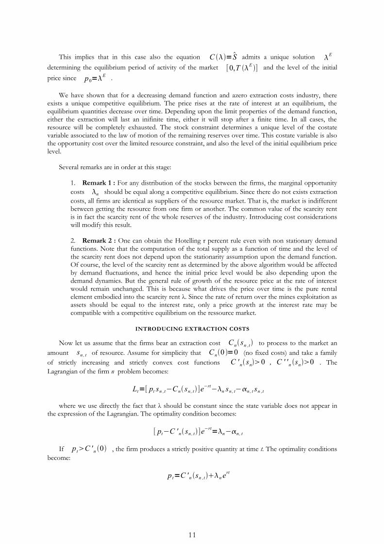
If p tC ' n 0 , the firm produces a strictly positive quantity at time t. The optimality conditions become:

p t=C ' n sn ,tn ert

11

Note that we get an extended version of the usual price-marginal cost equalization rule. Here, an efficient supply by the firm requires that the firm equalizes the price to the sum of the marginal cost of extraction and the marginal opportunity cost in current terms. This sum is sometimes called the full marginal cost of the exhaustible resource, the marginal opportunity cost standing as a depreciation cost of the mine asset to be covered at each time.

Hence the supply schedule of the firm is:

sn , t : solution of pt=C ' n sn ert if p tC ' n00 if p tC ' n0

The optimality condition defines implicitely sn , t≡sn pt ,n ,t . Now the opportunity costs of the various resources are different. The stock distribution will interfere with the determination of the scarcity rents over the different mines.

For the set of active firms N t , we get through the optimality conditions:

D ∑n∈N t

sn , t=p t=C ' n sn ,tnert

Differentiation of this relation gets:

D ' s td sn, t=C ' ' n sn, tdsn ,td n ertrn ert dt

From which we obtain:

∂ sn

∂n= ert

D ' s−C ' ' n sn , t0

∂ sn

∂ t=

r nert

D' s −C ' ' n sn ,t=r n

∂ sn

∂n0

The extraction rate of each active firm should decrease over time at the equilibrium. Hence the aggregate extraction rate should also decrease over time. Hence the equilibrium price should increase.

ds t

dt=∑

n∈N t

∂ sn

∂ t=r ert ∑

n∈N t

n

D ' s−C ' ' n sn , t0

d p t

dt=D ' s t

d st

dt=r ert ∑

n∈N t

D ' stn

D ' s−C ' ' n sn , t0

Since ∂ sn/∂ t0 , the marginal cost of extraction of each active mine should decrease over time. From the optimality conditions, we conclude that the equilibrium price should increase at a rate lower than the rate of interest. It appears that the simplest expression of the Hotelling rule, the r-percent rule, holds only in the zero extraction cost case. In more general case (for example with convex extraction costs), the equilibrium price should increase at a lower rate than the rate of interest.

Since the extraction rate decreases over time : sn , tn0=Max {sn ,t , tt n

0} where t n0 is the initial

extraction time (the beginning of the exploitation of the mine). Hence if the price is sufficiently high to

12

justify the exploitation of the mine, the same will be true thereafter, implying that each mine should be exhausted in a single phase exploitation period.

Note that there does not appear any single rule to determine the values of the marginal opportunity costs. The depend both upon costs functions and the stocks sizes distributions. An interesting exception is the linear cost case.

HERFINDHAL COST RULE

As shown by Herfindhal, under linear extraction marginal costs, the mines should be extracted in increasing marginal cost order. That is, the lowest cost mine should be exploited first followed by the second in cost order and so on. Let us consider N firms, each firm owns a stock of size Sn and extraction incurrs a unit cost cn . Index the firms by increasing cost order, that is :

c1c2...cn...c N . Price taking behavior from the firms implies that along any equilibrium;

p t=cnn ert , n∈N t⊂N

Note that if two firms n and n' produce simultaneously at the equilibrium, this should be the case that:

cn−cn '=n '−nert

Hence : cn 'cn , n 'n . The least cost deposit should have the highest rent at an equilibrium. In other words, a low cost resource deposit has a higher 'value', or a higher 'rent', than a more costly deposit.

But one notes also that such a relation cannot hold true for more than one instant. This implies that in fact, only only firm produces at a time. In other terms, the set of active firms is reduced to a singleton at each time. This may appear strange that we can speak of a competitive equilibrium where only one firm is producing at any given time. Competitive behaviour relies here heavily upon the price taking assumption. In this setting, the firms should recognize that they can act as monopolies and deviate from the price taking behavior, trying to extract more surplus from the users. If the firms behave in such a monopolistic way the equilibrium price path would be of course rather different.

Let us denote by t nn ,n1 the unique solution of:

cn1−cn=n−n1ert

this date is in fact the exhaustion date of the deposit n. That is over the time interval n≡[ t

n−1 , t n] , the firm n is the only firm supplying the resource market, until the deposit Snbecomes completely exhausted.

Let us remark that:

limt t n

d p t

dt=r n ert n

rn1ertn

=limt t n

d pt

dt

since we have shown that nn1 because cncn1 . This means that when the market forces put in use a higher cost deposit, the less costly deposit being depleted, the rate of growth of the equilibrium price should decrease at least initially. Symmetrically the rate of decrease of total ouput should also be lower in absolute terms.

13

Note also that the sizes of the stocks do not play any role in the determination of the scarcity rents. The price and total output dynamics look typically as shown on the following figure:

1: Fig Price and output dynamics in the Herfindhal model

Summary :

● A profit maximizing mining firm should organize the extraction over time in order to maintain constant in discounted terms the marginal profit of exploitation of the mine

● In current terms, the marginal profit should grow at the interest rate. This is the 'r-percent' rule for efficient mine exploitation

● Under efficient management, the value of the mine as an asset should decrease over time with the depletion of the stock. This decrease at one time period is approximatively equal to the current profit diminished by the rental value of the mine (the interest over the capital value of the mine)

● The rate of return of the mine over one time period is the ratio of the sum of current profit and rental value over the value of the mine at this time period. Under the 'r percent rule', the rate of

14

t1 t2 t3

pt = c2 + λ2 ert

price

time

st

return of the mine as a natural capital asset should be equal to the rate of return of other capital assets in the economy at an equilibrium over the financial market, that is the interest rate

● Without extraction costs, the competitive equilibrium price of the exhaustible resource should satisfy the simplest form of the Hotelling rule : the price should grow at the rate of interest.

● With convex costs (that is with increasing marginal costs functions), the equilibrium price of the resource should increase at a rate lower than the rate of interest.

● With linear unit costs function, the equilibrium order of exploitation of the mines should satisfy the Herfindhal order : the deposits must be sequentially depleted by increasing marginal cost order.

As we have seen, price taking behaviour of the firms may become conspicuous as in the case of constant unit costs, where only one firm may produce at a time along a competitive equilibrium. It is thus interesting to turn to the monopoly case.

EXTRACTION UNDER MONOPOLY

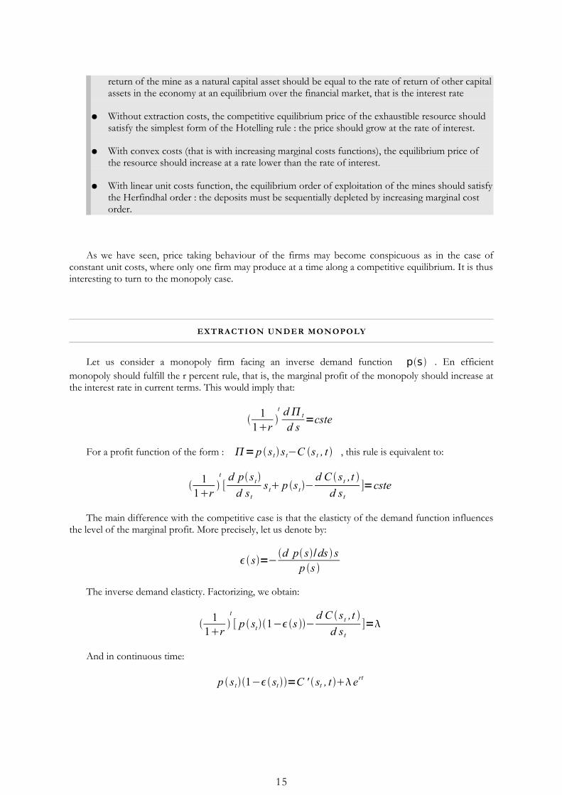
Let us consider a monopoly firm facing an inverse demand function ps . En efficient monopoly should fulfill the r percent rule, that is, the marginal profit of the monopoly should increase at the interest rate in current terms. This would imply that:

11r

t d t

d s=cste

For a profit function of the form : =p s t st−C s t , t , this rule is equivalent to:

11r

t

[d p s t

d s ts t p s t−

d C s t ,t d s t

]=cste

The main difference with the competitive case is that the elasticty of the demand function influences the level of the marginal profit. More precisely, let us denote by:

s=−d p s/ds sp s

The inverse demand elasticty. Factorizing, we obtain:

11r

t

[ p st1−s −d C s t ,t

d s t]=

And in continuous time:

p st1− st =C ' st , t ert

15

The main difference with the competitive market behaviour is that now, the equilibrium price dynamics is depending not only from the marginal cost dynamics and the scarcity rent dynamics, but also from the dynamics of the demand function elasticty.

Assume a demand function such that the elasticty is low for low levels of output and high for high levels of output. With the price rise over time, the monopoloy would face a demand lower and lower elastic. That is, the market power of the monopoly would be reduced through time. The capacity of the monopoly to contract the current supply to earn higher rents would thus be reduced. This should influence the extraction policy of the monopoly. With respect to the standard static monopoly case, the dynamic exhaustible resource monopoly earns two kinds of rents: a scarcity rent as the owner of a depletable asset and a market rent. The difficulty comes from the fact that these two sources of rents are linked together through the dynamics of the demand elasticity. This phenonomenon is particulary striking when ones considers the conservation issue.

MONOPOLY AND RESOURCE CONSERVATION

Since the usual tendancy of a monopoly is to reduce supply with respect to a competitive system, we should observe more conservative behaviour of the monopoly in resource management. By imposing higher prices for the resource than a competitive system, the monopoly should favor a lower pace of consumption of the natural resource over time, hence a lower rate of exhaustion and a more sustainable economy. In this sense, monopoly should be good for natural resource conservation.

This idea echoes recurrent debates in oil exploitation through history. In the interwar period, there were a recurrent debate in the United States about the oligopolistic behaviour of oil firms in this country. Facing a fastly growing demand, these firms were charged of being overly conservative, practicing high prices and underinvesting in exploration and the exploitation of new reserves. Some observers proposed to nationalize the oil fields for the citizen an consumer benefit. Other preferred to fight against what they judged being an « excessive » concentration in the oil sector, by dismantling existing firms and spreading their assets between a high number of small producers, favouring competition and lower prices. The oil firms answered to these critics by advocating their positive role as the best conservers of the non renewable resource asset, keeping into the ground more resources for the benefit of future generations of american people. This debate has been one of the motivation of the famous Hotelling essay (1931), the first to provide a rigourous analysis of the economic logic of exhaustible resources exploitation over time. This kind of critics appeared again during the sixties but in a rather different context. At that time, critics came from Middle East governments. For them, oil exploitation was a main opportunity to develop their countries. The anglo-american oil companies in charge of the exploitation of their reserves were accused to be overly conservative, and to systemmatically underinvest into the exploration and use of new oil fields. This is one of the argument put in front by Middle East governements to justify the nationalization of oil exploitation in their countries. The effect of the oil supply increase by the newly created national companies at the beginning of the seventies has been a price decrease. The objective behind the creation of OPEC at the same period was to counteract this adverse effect by using the monopoly power of a cartel to sustain higher prices. This resulted in the oil shocks of 1973 and 1979-80. The effect of the oil shocks has been finally to favour a demand drop, resulting in the counter oil shock. The loss of internal discipline inside the OPEC cartel followed the oil price drop. This shows that a monopoly can find an interest in producing more even in low prices periods because of an increased demand elasticty. Hence, it appears from these stylized facts, that the alleged 'conservative' behavior on the monopoly side may be at stake depending upon demand conditions.

We are going to show that if the demand function is isoelastic, the behaviour of the monopoly would be in fact exactly the same as those of a competitive industry. In other elasticity cases, many ambiguities appear, the idea of « overconservation » (or « underconservation ») being quickly blurred by different static and dynamic considerations.

16

Let us consider a monopoly which have to allocate a stock S to the supply of the market at two time periods, period 0 and period 1. Assume that the extractions costs are zero to simplify. The monopoly should equalize the discounted marginal profits over the two periods, that is set supplies

s0, s1 such that:

p s0d p s0

d s0s0=

11r

[ p s1d p s1

d s1s1]

Let R s be the marginal revenue function:

R s =p sd p sds

s=p s1− s

Assume that the marginal revenue is a decreasing function of output (note that the concavity of the inverse demand function is a sufficient but not necessary condition for that). In the case of an isoelastic demand function : s= . The profit maximizing condition of the monopoly becomes :

R s0=1

1rR s1

p s01−=1

1r p s11−

p s0=1

1r p s1

This is the canonic form of the Hotelling rule applying in a competitive context. Hence if the price levels would be different under monopoly and under competition, the output delivered to the market at the two periods would be the same in the two market structures. This is illustrated on the following graph:

2: Fig Monopoly versus competition in the isoelastic case

17

p(s)(1/(1+r))

R(s)(1/(1+r))

p(s)R(s)

pc0

pc1/(1+r)

pm1/(1+r)pm

0

Ŝsc0=sm

0 sc1=sm

1

In the competitive market structure the stock allocation over the two time periods s0,c s1

c is determined by the intersection between the demand schedule for period 0 and the discounted demand schedule for period 1. The competitive equilibrium price satisfies the Hotelling rule, that is :

p0c=1/1r p1

c . In the monopoly market structure, the stock allocation over the two time periods s0,

m s1m is determined by the intersection between the marginal revenue schedule for period 0

and the discounted marginal revenue schedule over the period 1. Since the demand has a constant elasticity, the Hotelling rule should also apply to the monopoly price (beware : this is true only in this specific case !!), hence : p0

m=1/ 1r p1m . Note that in this case, the monopoly price should be

lower than the competitive price but the quantities supplied to the market at the two periods should be the same in the competitive regime and in the monopoly regime, that is s0

c=s0m and s1

c=s1m . Of

course, the total amount of resource must be depleted over the two periods, that is : s0

cs1c=s0

ms1m=S . To check that, it is necessary and sufficient to prove that the system:

p s0=1

1r p s1

s0s1=S

admits only one solution. Using the stock constraint, this is equivalent to show that the equation:

p s= 11r

p S−s

has an unique solution. Assume that p S 1r p 0 . Let:

s =1r p s −p S−s

Since the demand function is decreasing in s, 0=1r p 0−p S p 0− p S 0and under our previous assumption : S =1r p S − p00 . Moreover:

d s ds

=1r d p s ds

d p S−s

ds0

Hence, the equation s =0 has a unique solution.

If the elasticity of the demand function varies along the demand curve, it is easily verified that:

d s ds

0 s0ms0

c , s1ms1

c

and the converse applies when the elasticity of the inverse demand function is decreasing alon the inverse demand curve. With respect to a competitive industry, the monopoly will contract its supply at the first period and this will imply to sell more than the competitive industry in the second period.

These results can be easily extended to the continuous case. As seen before the basic optimality condition for the setting of a supply plan by the monopoly in the zero extraction cost case is the following:

p st1− ste−r t=

18

A logarithmic differentiation through time gets:

p t

p t=r

d s ds

11−s

With an isoelastic demand function, we get back the familiar Hotelling rule : the monopoly price should grow at the interest rate. If the elasticity is higher for high outputs than for low outputs (increasing eleasticity), the price should grow at a higher rate, and conversely, if elasticty is lower for high outputs (decreasing elasticty), the price should grow at a lower rate than the rate of interest.

But this is not sufficient to obtain a definite conclusion with respect to the monopoly behaviour compared to a competitive situation in terms of the resource conservation. We need to give a more precise statement of what is a « more conservative behaviour ». Assume that lim s 0 D s=p∞ . This maximal level of the resource price compatible with a strictly positive level of output in equilibrium is sometimes called the choke-off price. Under this assumption, the resource should be exhausted in finite time under our cost assumptions. Using this finite time property, we can give a definition of a « conservative » behaviour. We shall define :

● A market structure is « more resource conservative » than another if the exploitation length is longer along a dynamic equilibrium.

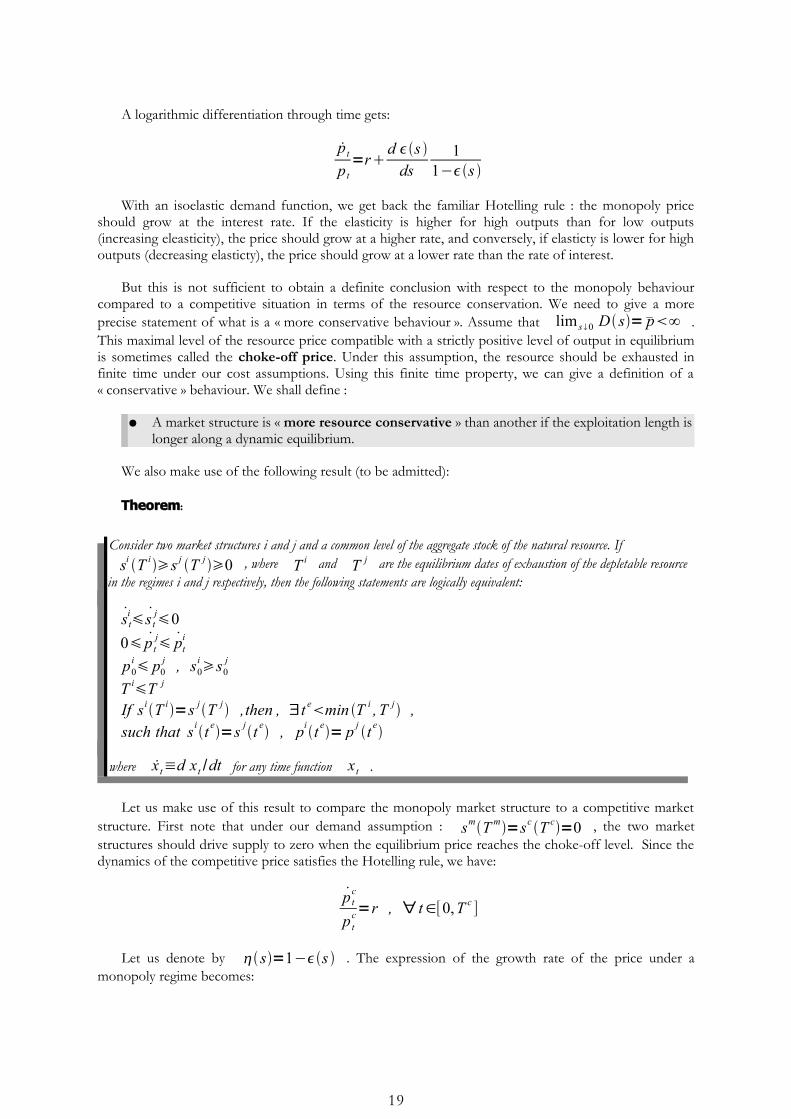
We also make use of the following result (to be admitted):

:Theorem

Consider two market structures i and j and a common level of the aggregate stock of the natural resource. If si T is j T j0 , where T i and T j are the equilibrium dates of exhaustion of the depletable resource

in the regimes i and j respectively, then the following statements are logically equivalent:

s ti s t

j00 p t

j pti

p0i p0

j , s0is0

j

T iT j

If siT i=s jT j ,then , ∃ t emin T i , T j ,such that sit e=s jt e , pit e= p j t e

where x t≡d xt /dt for any time function x t .

Let us make use of this result to compare the monopoly market structure to a competitive market structure. First note that under our demand assumption : smT m=sc T c=0 , the two market structures should drive supply to zero when the equilibrium price reaches the choke-off level. Since the dynamics of the competitive price satisfies the Hotelling rule, we have:

p tc

p tc=r , ∀ t∈[0,T c ]

Let us denote by s=1−s . The expression of the growth rate of the price under a monopoly regime becomes:

19

p tm

p tm=r−

t

t

Using the previous theorem, we know that there exists some instant t e where p tem= p te

c≡ pt e . Hence at this time:

p tem

p tem−

pt ec

pt ec =

pt em− p te

c

p te

=−t e

t e

Let us consider the case of an increasing inverse demand elasticity, that is a demand more elastic for high levels of output than for low levels of output. Since output should decrease over time along an equilibrium, this would imply that the elasticity should decrease over time and hence that t0Hence, we conclude that at time t e :

p tem− p te

c0

Using the main theorem we conclude that T cT m , the monopoly is more conservative than a competitive extractive industry. Furthermore : p0

c p0m and s0

cs0m , that is the monopoly sets an

higher initial price and produces less initially. The monopoly is more conservative initially in the static sense, contracting output. But after t e , p t

m ptc and s t

ms tc , the monopoly would be less

conservative than a competitive industry in the static sense, producing more and setting lower prices. However, as we have shown, in the dynamic sense, the monopoly appears as more conservative than a competitive system, since it depletes the resource over a longer time duration. The following graph illustrates the comparative price dynamics:

3: Fig Monopoly and competitive price dynamics when elasticity is lower for high levels of output

20

te Tc Tm time

p

pm0

pc0

pct

pmt

DUOPOLIES

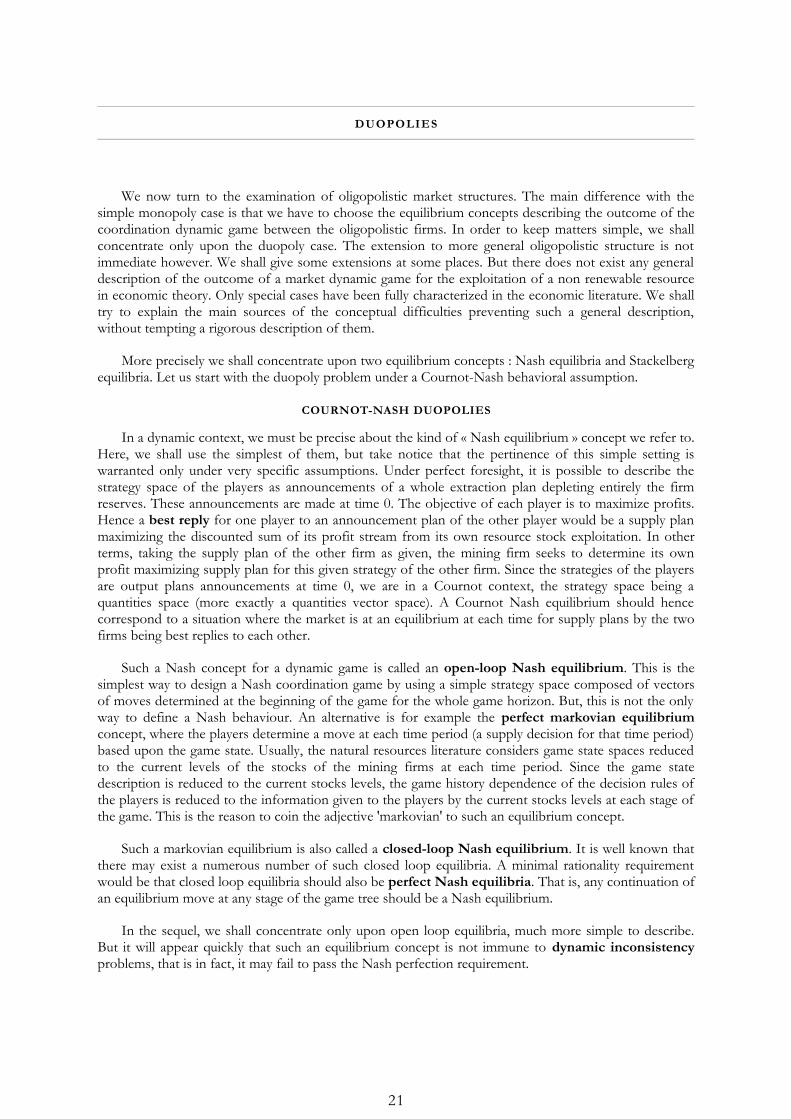
We now turn to the examination of oligopolistic market structures. The main difference with the simple monopoly case is that we have to choose the equilibrium concepts describing the outcome of the coordination dynamic game between the oligopolistic firms. In order to keep matters simple, we shall concentrate only upon the duopoly case. The extension to more general oligopolistic structure is not immediate however. We shall give some extensions at some places. But there does not exist any general description of the outcome of a market dynamic game for the exploitation of a non renewable resource in economic theory. Only special cases have been fully characterized in the economic literature. We shall try to explain the main sources of the conceptual difficulties preventing such a general description, without tempting a rigorous description of them.

More precisely we shall concentrate upon two equilibrium concepts : Nash equilibria and Stackelberg equilibria. Let us start with the duopoly problem under a Cournot-Nash behavioral assumption.

COURNOT-NASH DUOPOLIES

In a dynamic context, we must be precise about the kind of « Nash equilibrium » concept we refer to. Here, we shall use the simplest of them, but take notice that the pertinence of this simple setting is warranted only under very specific assumptions. Under perfect foresight, it is possible to describe the strategy space of the players as announcements of a whole extraction plan depleting entirely the firm reserves. These announcements are made at time 0. The objective of each player is to maximize profits. Hence a best reply for one player to an announcement plan of the other player would be a supply plan maximizing the discounted sum of its profit stream from its own resource stock exploitation. In other terms, taking the supply plan of the other firm as given, the mining firm seeks to determine its own profit maximizing supply plan for this given strategy of the other firm. Since the strategies of the players are output plans announcements at time 0, we are in a Cournot context, the strategy space being a quantities space (more exactly a quantities vector space). A Cournot Nash equilibrium should hence correspond to a situation where the market is at an equilibrium at each time for supply plans by the two firms being best replies to each other.

Such a Nash concept for a dynamic game is called an open-loop Nash equilibrium. This is the simplest way to design a Nash coordination game by using a simple strategy space composed of vectors of moves determined at the beginning of the game for the whole game horizon. But, this is not the only way to define a Nash behaviour. An alternative is for example the perfect markovian equilibrium concept, where the players determine a move at each time period (a supply decision for that time period) based upon the game state. Usually, the natural resources literature considers game state spaces reduced to the current levels of the stocks of the mining firms at each time period. Since the game state description is reduced to the current stocks levels, the game history dependence of the decision rules of the players is reduced to the information given to the players by the current stocks levels at each stage of the game. This is the reason to coin the adjective 'markovian' to such an equilibrium concept.

Such a markovian equilibrium is also called a closed-loop Nash equilibrium. It is well known that there may exist a numerous number of such closed loop equilibria. A minimal rationality requirement would be that closed loop equilibria should also be perfect Nash equilibria. That is, any continuation of an equilibrium move at any stage of the game tree should be a Nash equilibrium.

In the sequel, we shall concentrate only upon open loop equilibria, much more simple to describe. But it will appear quickly that such an equilibrium concept is not immune to dynamic inconsistency problems, that is in fact, it may fail to pass the Nash perfection requirement.

21

Let us consider a duopoly composed of two mining firms labelled 1 and 2 and endowed initially with given stocks of an homogeneous non renewable resource S1 and S2 respectively. By an « homogeneous » resource, we mean a mineral resource of a given common quality perfectly substituable at the consumption level. Assume without loss of generality that S1 S 2 . We are facing a non symmetric duopoly problem since the two initial stocks levels are different. For the sake of simplicity assume also that the extraction costs are zero, that is consider a pure rental problem of resource exploitation over time. Let us denote by si ,t the supply decision of the firm i at time t, i=1,2, and by

s t=s1, ts2, t the corresponding aggregate supply at time t. Let p= p s be the inverse demand function and assume that p ' s 0 , s0 and lim s 0 p s =p∞ . This would imply a finite time operation duration of the industry at an equilibrium.

As stated before, we want to apply the open-loop Nash equilibrium concept. That is, each firm must determine a supply plan and a termination date maximizing the discounted sum of profits from the mine exploitation taking the supply plan of the other firm as given. In the case of firm 1 for example, this problem may be written formally as such:

Max {s1, t } ,T 1∫

0

T 1

[ p s1, ts 2, t s1, t]e−rt dt

s.t. S1,t=−s1, t , S1,0= S 1 , s1, t0 , S 1, t0 , t∈[0,T 1]

The Lagrangian of this problem is the following:

Lt= p s t s1, t e−rt−1 s1, t1, t s1, t

where we exploit the fact that the state variable does not appear into the expression of the Lagrangian to impose directly that the costate variable should be a constant 1 . Performing the same calculation for the other firm, we get the following system of optimality conditions for the two firms:

p ' s t s1, t p s t=1−1, tert

p ' s t s2, t p s t=2−2, tert

Let us denote by 1, t and 2, t=1−1, t the market shares of the two firms, that is i ,t=si ,t /s t for i∈{1,2} . Let us concentrate upon a time interval where the two firms

would simultaneously produce. Introducing the direct demand elasticity 1/ s=−p ' s s / p s the system may be rewritten as:

p st1−1, t

s t=

p stst

st−1, t=1 ert

p st1−2, t

s t=

p st st

st −2, t=2 ert

We obtain through a logarithmic differentiation through time:

p t

p t−t

tt−1, t

t−1, t=r=

p t

p t−t

tt−2, t

−2, t

Identifying and recalling that since: 2, t=1−1, t , 2, t=−1, t , we obtain:

22

t {1

t−1, t− 1t−2, t

}=1, t {1

t−1, t 1t−2, t

}

t {t− 2, t−t1, t

t−1, tt−2, t}=1, t {

t−2, tt−1, t

t−1, tt− 2, t}

t1, t−2, t=1, t 2−1

THE ISOELASTIC CASE

In the isoelastic case, t=0 implies that 1,t=2,t=0 . Hence the market shares of the two firms should remain the same over . From the above relations, note also that: p t / pt=r , the equilibrium price should grow at the rate of interest, the basic formulation of the Hotelling rule. But since the market shares are constant, this implies also that the two firms should exhaust their stocks during the same time interval, that is: T 1=T 2=T . We get also:

s1, t=1 st=1

22 st=

1

2s2, t

The extraction rates should be proportional along the equilibrium path. Since the stocks must be depleted over the same time period:

S1=∫0

T

s1,t dt=1

2∫0

T

s2,t dt=1

2

S 2

which gives:

1=S1

S 1 S2

12

Since the firm 1 has a greater stock than the firm 2, its market share should be higher. Form the first order condition note that this implies that 12 , the scarcity rent of the most important firm should be lower than the scarcity rent of the smallest firm. The smallest firm enjoys a higher rent level than its competitor.

THE VARIABLE ELASTICITY

CASE

Let us suppose that 12 . This would imply from the first order conditions that:

p ' s t s1, t p st=1 ert2 ert=p ' s t s2, t p stp ' st s1, t p ' s t s2, t

s1, ts2, t

23

Furthermore, the choice of the termination date T i , i=1,2 must verify the following « transversality condition »:

H T i=0 , pT i

si ,T ie−rT i−i si ,T i

=0

This implies that: pT i=i e

rT i , i=1,2 . We conlude that if 12 we should have

pT 1e−rT 1pT 2

e−r T2 . But since the ressource price should grow at a rate lower than the rate of interest, this would imply that p t e

−rt decreases through time and hence that T 1T 2 . Hence the firm 1 should extract less during a shorter duration, which is impossible since the firm 1 has the largest stock by assumption. We conclude that :

S1 S 2 12

The scarcity rents should be ranked in inverse order with the initial stocks distribution.

But if 12 we infer that, first, 1, t2, t , t∈ , the largest firm should have a higher market share, and second, T 1T 2 , the largest firm should enjoy a monopoly position after its smaller opponent has completely depleted its own reserves. We have here a hint to an underlying dynamic consistency problem. The exploitation profile will be composed of a first duopoly phase followed by a monopoly phase. Note that the market structure is endogenous, that is the termination date of the smallest firm will be endogeneously determined by the market forces and the strategic chooses of the two firms. We see that the dominant firm has an incentive to push its opponent to exhaust quickly its own reserves in order to enjoy a monopoly position for a longer time. We shall go back to this point later. From our previous calculations we can now conclude that during the first duopoly phase:

,= ,0 1, t ,=,0

The largest firm will increase over time its market share if the elasticty increases over time. It is easily checked that total supply should decrease during the dupoly phase. Hence if the elasticity increases over time this means that the inverse demand function would become less elastic for low levels of output with respect to high levels of output.

A LINEAR DEMAND FUNCTION

EXAMPLE

Let us assume that the inverse demand function is of the linear form:

p s=a−b s , a0 , b0 , p 0=a≡p

We are in the context of our initial assumptions, the inverse demand function is a strictly decreasing function and the choke-off price is equal to a. The duopoly system at any time t∈ becomes:

−2b s1a−b s2=1 ert

−2b s2a−b s1=2 ert

24

For a given 1,2 pair, we deduce the best reply functions to the output decision of the other firm:

s1 s2, t =−12

s2a−1e

rt

2b

s2 s1, t =−12

s1a−2e

rt

2b

Note that the best reply functions are decreasing functions of the other firm decision and time.

Next, differentiate through time the first order conditions system and obtain:

−2b s1−b s2=r [−2b s1a−b s2]−2b s2−b s1=r [−2b s2a−bs1]

Multiply by (-2) the first equation, add the result to the second one and get:

s1=r s1−ar3b

a linear with constant coefficients first order ordinary differential equation in s1 only. A particular solution is s1=kert which after insertion into the previous relation gives: k t=−ar /3be−rt . Integrating over [ t ,T 1] this gives:

k T 1−k t=

a3b[e−rT 1−e−rt ]

Since we conclude that k T 1=0 . Hence we obtain:

s1, t=a3b[1−e−r T 1−t]

It remains to compute the value of T 1 . Using the stock condition we get:

S1=∫0

T1

s1, t dt= a3b∫0

T 1

1−e−r T 1−tdt= a3b[T 1−

1−e−rT 1

r]

Let f x =x−1−e−r x/r . Note that:

f 0=0 , f ' x=1−e−rx0 , f ' ' x=r e−rx0 , lim x ∞ f x =∞

Hence the stock condition defines implicitely a function T 1=T S 1 where lim S 0 T S =0, lim S ∞ T S =∞ , and d T S /dS0 . We can perform analogous computations for the other firm supply and get:

s2, t=a3b[1−e−r T 2−t ] , S 2=

a3b[T 2−

1−e−rT 2

r]

25

sT 1=k T1

erT1=0

Assume that S1 S 2 . From the properties of the function T S we conclude that T 1T 2 . Hence the equilibrium path is composed of two sucessive phases, a first duopoly phase,

terminated by the exhaustion of the stock of the firm 2, [0,T 2 ] , and a second monopoly phase [T 2, T 1] where only the firm 1 produces.

The above result requires to modify the computation of the output function s1, t . During the monopoly phase, the optimality condition implies that:

p ' s1, t s1, t p s1,t=a−2b s1, t=1ert

Since at the termination time, s1, T1=0 , we obtain : 1=ae−rT 1 . Hence the output of firm 1

during the monopoly phase is given by:

s1, t=a

2b[1−er t−T1 ] , t∈[T 2,T 1]

Next, integrating the differential equation defining the dynamics of s1, t during the initial duopoly phase [0,T 2] , we get:

k t=kT 2 a

3b[e−r t−e−rT 2]

Hence, since s1, t=k t ert :

s1, t=s1,T 2er t−T2 a

3b[1−er t−T 2] , t∈[0,T 2]

By continuity with the following monopoly phase, we obtain:

s1, T2= a

2b[1−er T2−T 1]

Hence the correct expression of s1, t during the dupoloy phase is in fact:

s1, t=a

2b[e−r T2−e−rT 1]er t a

3b[1−er t−T 2] , t∈[0,T 2]

Remember that T 2=T S 2 , hence only T 1 remains to be determined to get a complete characterization of the equilibrium path. Note that the second term of the sum is in fact equal to s2, t , hence :

s1, t=a

2b[e−r T2−e−rT 1]erts2,t

As seen before the market share of the dominant firm 1 is higher than the market share of the other firm. In this example, the differential between the outputs increases at the insterest rate and is an increasing function of the duration of the monopoly phase.

Next, introducing the stock condition, we obtain:

26

S1=∫0

T2

s1, t dt∫T 2

T 1

s1, t dt

That is:

S1=∫0

T2

[ a2b

e−rT 2−e−rT 1erts2,t]dt∫T 2

T 1 a2b

[1−er t−T1 ] dt

equivalent to:

S1=a

2b e−r T 2−e−rT 1

erT 2−1r S 2

a2b [ T 1−T 2−

1−er T2−T 1

r ]

Developping and rearranging, we get:

S1= S 2a

2b[T 1−T 2−

1−er T 2−T 1

r1−er T 2−T 1

r1−e−rT 2]

Simplifying and rearranging again:

S1= S 2a

2b[T 1−T 2

e−r T1−e−rT 2

r]

Let g T 1 be the expression appearing at the RHS of the above equation. We get for T 1=T 2 , g T 1=T 2= S 2 and:

g ' T 1=a

2b[1−e−rT 1]0 , g ' ' T 1=

a r2b

e−rT 10

Furthermore limT 1∞g T 1=∞ . Hence the equation g T = S1 admits a unique solution

T 1 S1, T S 2 .

Using the second optimality condition evaluated at t=T 2 :

−2b s2,T2a−b s1,T 2

=a−b a2b

e−rT 2−e−r T1erT 2=a−a21−er T 2−T1 =a

21er T 2−T1

Hence:

a21er T 2−T 1=2 erT 2 , 2=

a2e−r T2e−rT 1

Since T 2T 1 and 1=ae−rT 1 we obtain:

2−1=a2[e−rT 2−e−rT1]0

27

We have checked that 12 if S1 S 2 . The following system defines implicitely 1 S1,

S 2 and 2 S1,S2 .

1=a e−rT 1 S 1,S 2

2=a2e−rT 2 S2 e−rT 1 S 1,

S 2

Total differentiation gets:

d 1=−a r e−r T 1∂T 1

∂ S1

d S 1−a r e−rT 1∂T 1

∂ S 2

d S 2

d 2=a2[−r e−r T 1

∂T 1

∂ S 1

d S 1−r e−r T 2∂T 2

∂ S2

e−rT 1∂T 1

∂ S2

d S 2]

In matrix form:

[−a r e−rT 1∂T 1

d S 1

−ar e−rT 1∂T 1

∂ S 2

−a r2

e−rT1∂T 1

∂ S 1

−ar2e−rT 2

∂T 2

∂ S2

e−rT 1∂T 1

∂ S 2

][d S 1

d S 2]=[ d 1

d 2]

We must first compute the derivatives of the termination dates with respect to the initial stocks. For T 2 use the stock condition:

S2=a

3b[T 2−

1−e−rT 2

r]

Totally differentiating, we obtain:

d S2=a

3b[1−e−r T 2] d T 2

∂T 2

∂ S2

= 3ba 1−e−r T1

For T 1 , we get:

S1−a

2bT 1

e−r T1

r= S 2−

a2b

T 2e−rT 2

r

Totally differentiating results in:

d S1−a

2b1−e−rT 1d T 1=d S 2−

a2b

1−e−r T 2∂T 2

∂ S2

d S2

Inserting the expression of ∂T 2/∂ S2 we obtain:

28

d S1−a

2b1−e−rT 1d T 1=d S 2[1−

a2b

1−e−r T2 3ba 1−e−rT 2

]=−d S 2

2

Hence we get the following expressions of the partial derivatives:

∂T 1

∂ S 1

= 2ba 1−e−r T1

0 ,∂T 1

∂ S 2

= ba 1−e−rT 1

0

The determinant of the first matrix in the differntial system is:

D=ar 2

2{e−r T1T 2 ∂T 1

∂ S1

∂T 2

S 2

e−2 r T1∂T 1

∂ S 1

∂T 1

∂ S 2

−e−2 r T1∂T 1

∂ S 1

∂T 1

∂ S 2

}

D=a r 2

2e−r T 1T 2 ∂T 1

∂ S 1

∂T 2

∂ S2

0

Using the Cramer rule we obtain:

∂1 S1,S2

∂ S 1

= 1D ∣1 −

0 −∣=−D

0

∂1 S1,S2

∂ S 2

= 1D ∣− 1− 0∣=−−D

0

It appears that the scarcity rent over the stock of the firm 1 is a decreasing function of the stock size of the firm and an increasing function of the stock size of the other firm. Using the same technique for the scarcity rent of the firm 2, we get:

∂2 S1,S 2

∂ S1

= 1D∣0 −

1 −∣=−−D

0

∂2 S1,S 2

∂ S 2

= 1D∣− 0− 1∣=−

D0

Hence, we obtain the same results. It is important to keep in mind that the scarcity rents ar simultaneously determined hence they should depend upon both initial stocks. The scarcity rents do not measure some « absolute » scarcity but the relative scarcity of the resources. Hence the scarcity value of one stock should depend upon the availability of the other stock. The scarcity measure of one stock is reduced if this stock is increased (the availability is higher) and increased if the other stock is increased (the stock becomes more scarce in relative terms with respect to the increased other stock).

The following graph illustrates the determination of the spot equilibrium. The best reply functions are decreasing lines in the s1, s2 space.

29

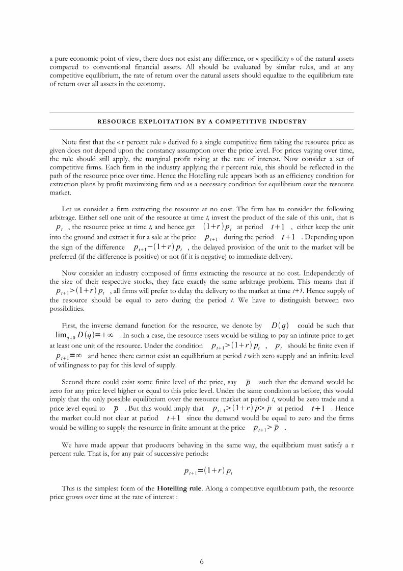
4 : Fig Cournot Nash spot equilibrium

Over time, the slopes of these lines remain the same (equal to ½ for s2(s1) and to 2 for s1(s2)). But the constant decreases over time. Hence the best reply lines translate downwards through time, their intersection describing the equilibrium path over time, as illustrated upon the following picture:

5 : Fig Dynamics of the Cournot Nash equilibrium

30

s1(s2)

s2(s1)

s*1

s*2

s1

s2

Duopoly phase [0,T2]

Monopoly phase [T1,T2]

s1

s2

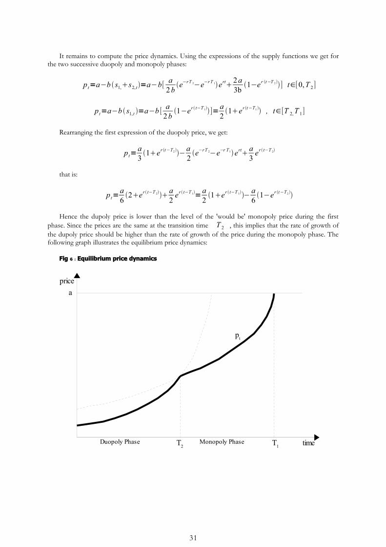
It remains to compute the price dynamics. Using the expressions of the supply functions we get for the two successive duopoly and monopoly phases:

p t=a−b s1,s2, t=a−b[ a2b

e−rT 2−e−rT 1ert2a3b

1−er t−T 2 ] t∈[0,T 2]

p t=a−b s1, t =a−b [ a2b

1−er t−T 1]=a21er t−T1 , t∈[T 2, T 1]

Rearranging the first expression of the duopoly price, we get:

p t=a31er t−T2 −a

2e−rT 2−e−r T1erta

3er t−T 2

that is:

p t=a62er t−T 2a

2er t−T 1=a

21er t−T 1− a

61−er t−T2

Hence the dupoly price is lower than the level of the 'would be' monopoly price during the first phase. Since the prices are the same at the transition time T 2 , this implies that the rate of growth of the dupoly price should be higher than the rate of growth of the price during the monopoly phase. The following graph illustrates the equilibrium price dynamics:

6 : Fig Equilibrium price dynamics

31

Duopoly Phase T2 T1Monopoly Phase

a

pt

time

price

CARTEL VERSUS COMPETITIVE FRINGE

Most attempts to modelize the oil market rely on a description involoving two main kinds of firms (or countries). On one side, major producers are cartelized inside the OPEC and coordinates their extraction policy with the objective of keeping high prices. They are under competition from minor producers, behaving in a competitive manner. The small producers form a competitive fringe reducing the monopoly power of the OPEC cartel. Historically, this was more the lack of internal discipline inside the cartel which explained the low oil prices after the counter oil shock than the competititive pressure coming from the fringe. Composed mainly of US producers and Northsea countries (Scotland, Norway), the fringe was too small with respect to the OPEC countries to have a significant impact upon price formation on the oil market. The rise of Russia and other Central Asia producers since the end of the nineties is now challenging this historical segmentation of the oil market, the « fringe » becoming more and more the market core and the OPEC being again submitted to internal pressures to increase output in a high energy price context driven by emergent countries growing demand.

As we have seen before, a dominant firm should enjoy a monopoly position after the depletion of its oppoent reserves. Instead of adopting the cautious Cournot-Nash behaviour, taking the production of the other as given, the dominant firm could adopt a more active behaviour, taking into account the reaction of the competitors to its own supply policy and incorporating this reaction as a constraint in its own profit maximization problem. Such a behaviour of the dominant firm is called a Stackelberg behaviour. In such a Stackelberg game, the cartel acts as a Stackelberg leader on the resource market, the producers inside the competitive fring being Stackelberg followers. A Stackelberg game is in fact a hierarchical Nash game, where the dominant player takes the best reply function of the other player as given, instead of taking as given any strategy profile the follower could choose.

We are going to constrast the outcome of such a Stackelberg game with the preceding analysis of a Cournot-Nash duopoly. Let us assume that there exists N producers owning initially the same individual reserve S . The cartel is composed of nc producers and the fringe of n f producers, hence

ncn f =N . Assume that ncn f , hence Sc≡ncSn f

S≡ S f , the total size of the reserves controlled by the cartel is higher than the fringe aggregate reserves.

Assume zero costs of extraction and let us take the example of a linear inverse demand function : p s=a−bs=a−b scs f where p denotes the resource price, s is total output and sc , s f

are the cartel and fringe production respectively. It may be easily checked that in such situations, the cartel should enjoy a monopoly power phase after the exhaustion of the fringe reserves. More precisely the Stackelberg equilibrium path will be composed of a first phase [0,T f ] during which the cartel and the fringe both supply the market, followed by a monopoly phase [T f , T c ] where the cartel remains the sole supplier. T f ,T c are the termination dates of the fringe and the cartel respectively.

Let us first consider the monopoly phase. As seen before, equilibrium production and price are given by the following relations:

sc ,t=a

2b1−er t−T c , t∈[T f , T c ]

p t=a21er t−Tc , t∈[T f , T c ]

Note that under our demand assumptions, the cartel policy during the monopoly phase fulfills what is called the « non reentry condition » by the fringe. Acting as a competitive producer, the fringe should determine its supply policy in order to satisfy the simple Hotelling rule, that is the equilibrium price

32

should grow at the rate of interest along any time interval the fringe would choose to supply the market. In order to prevent fringe producers to keep some fraction of their reserves into the ground after T f , the cartel should set a supply policy for which the corresponding price grows at a rate lower than the rate of interest. Doing so, the fringe producers have no incentive to come back to the market depleting their remaining reserves. This condition is the « non reentry condition » and may be simply stated as :

p tp t fer t−T f , t∈[T f ,T c ]

Under our demand framework, this condition is always verified by the optimal monopoly policy over [T f , T c ] . Let us compute c , the optimal monopoly profit over the monopoly phase.

c≡∫T f

T c

pt sc ,t e−rt dt=∫

T f

T c a21er t−Tc a

2b1−er t−T ce−rt dt

c=a2

4b∫T f

T c

1−e2r t−Tc e−rt dt= a2

4b∫T f

T c

e−rt−er t−2 T cdt

c=a2

4b[− e−rT c−e−r T f

r− e−r Tc−er T f−2T c

r]= a2

4b r[e r T f−2T c−2 e−r Tce−rT f ]

c=a2

4 bre−rT f [e2r T c−T f −2 e−r T c−T f 1]= a2

4bre−rT f [1−e−r T c−T f ]2

Let us denote by T≡T c−T f , the length of the monopoly phase. Using the stock condition:

Sc , T f=∫

T f

T c

sc ,t dt=∫T f

T c a2b

1−er t−T cdt= a2b

[T−1−e−r T

r]

This relation determines implicitely T=T S c ,T f . Hence the maximized profit over the

monopoly phase is itself determined as a function of T f and Sc , T f:

c=c T f , S c ,T f= a2

4bre−rT f [1−e−r T S c,T f

]2

such that:∂c

∂T f0 ,

∂c

∂ S c , T f

0 . The monopoly profit of the cartel is increased if the cartel

manages to have the fringe exhausting quicker in time its reserves (thus reducing T f ), or if it owns a higher level of remaining reserves at the end of the duopoly phase. But, in order to have the fringe selling more during the first phase (and thus exhaust quicker its reserves), the equilibrium price should be lower, implying that the cartel too has to increase its production. Hence there is a trade-off for the cartel between enjoying a longer monopoly position and disposing of high reserves at the beginning of this phase.

Next, examine the first duopoly phase. The cartel, as a Stackelberg leader, should internalize the reaction of the fringe to its supply decisions. But in the zero cost case, the competitive supply of the fringe is indeterminate, the only constraint being that the equilibrium price should fulfill the Hotelling rule, that is the price should grow at the rate of interest. And since the price path is a continuous function of time at the termination date T f :

33

p t=pT fer t−T f =a

21er T f−T cer t−T f = a

2e−rT f 1e−r T ert

The cartel problem is the following:

Max∫0

T f

[ p t sc , t]e−rt dtc

s.t.˙Sc , t=−sc ,t ˙S f ,t=−s pt sc , t , pt=r pt

s f ,T f=0

This is a rather complex control problem with three state variables. However, under our assumptions, this problem can be transformed into a static optimization problem in the two variables

T f and Sc , T f. Inserting the expression of the price into the profit function results in:

=∫0

T f a21e−r T e−rT f ert sc , t e

−rt dtc

That is:

=a21e−rT e−r T f∫

0

T f

sc , t dtc=a21e−r T e−rT f S c−S c ,T f

c

which allows to express the cartel objective as a function of T f , Sc ,T f :

T f , S c ,T f=a

21e−rT S c ,T f

e−rT f Sc−S c ,T f a2

4bre−rT f 1−e−r T S c,T f

2

Moreover, we obtain from the expression of the price path:

p t=a−bs t=a21e−rT er t−T f

Integrating over [0,T f ] gets:

∫0

T f

pt dt=aT f−b S c−S c ,T f S f =

a21e−r T 1−e−rT f

r

Hence the profit is equal to:

T f , S c ,T f=

br e−r T f ab

T f− S cS c ,T f− S f S c−S c ,T f

1−e−rT f

a2

4br e−rT f 1−e−r T 2

The optimal choice of Sc , T fmust verify: ∂/∂ S c ,T f

=0 hence:

34

∂∂ Sc , T f

= bre−rT f

1−e−rT f[1 S c−S c ,T f

ab

T f− S cS c ,T f− S f −1]

a2

4br e−rT f 21−e−rT r∂T∂ S c ,T f

e−r T =0

Differentiating the stock condition over the monopoly phase gets:

d Sc , T f= a

2b[1−e−r T ]dT

∂T∂ S c ,T f

= 2ba 1−e−r T

Hence we obtain:

∂∂ Sc , T f

= br e−rT f

1−e−r T f[ Sc−Sc ,T f

− a2b1e−r T 1−e−r T f

r]

a2

4b re−rT f 1−e−rT 4b r e−rT

a 1−e−r T =0

which simplifies to:

br1−e−r T f

[ S c−S c ,T f− a

2b1e−rT 1−e−rT f

r]=−a e−r T

That is:

S c−Sc , T f=− a

bre−rT 1−e−r T f a

2br1e−r T 1−e−r T f

Rearrange to obtain:

S c−Sc , T f= a

2b r1−e−r T f [−2e−rT1e−rT ]= a

2br1−e−r T f 1−e−rT

Next, coming back to the stock condition during the duopoly phase, we get:

S f=ab

T f− S c−S c , T f− a

2b1e−rT 1−e−r T f

r

which, using the expression of Sc−Sc ,T f, gives:

S f=ab

T f−a

2br1−e−rT f 1−e−r T1e−r T = a

b[T f−

1−e−rT f

r]

This relation determines in a unique way T f S f , the end time of the duopoly phase uniquely as a function of the fringe reserves. Note that d T f S f /d S f 0 , the length of the duopoly phase increases with the importance of the fringe reserves.

Next, let us consider again the stock conditions over the duopoly phase and the monopoly phase:

35

Sc−Sc ,T f= a

2b1−e−r T f 1−e−rT

r

S c ,T f= a

2b[T c−T f−

1−e−r T

r]

Sum up these two relations to obtain:

2 Sc=ab [T c−T f1−e−r T f−1 1−e−r T

r ]=ab [T c−T f −

e−rT f−e−rT cr ]

Adding and substracting 1 results in:

2 Sc=ab[T c−T f−

e−rT f−1r

−1−e−rT c

r]

but recalling the expression of T f S f :

2 Sc=ab[T c−

1−e−rT c

r]−a

b[T f−

1−e−rT f

r]=a

b[T c−

1−e−rT c

r]− S f

which gives:

2 Sc S f=ab[T c−

1−e−r T c

r]

determining in a unique way a function T c Sc , S f , both increasing in the cartel and the fringe reserves.

It is possible now to contrast the Stackelberg equilibrium and the Cournot Nash solution. Endow the cartel and the fringe with the same reserves distribution as the duopoly player of the Cournot Nash game. Let us first consider the duration of the duopoly and monopoly phases.

For the duration of the duopoly phase, we get:

S 2=abT 2

S−1−e−r T 2S

r

3 S 2=abT 2

N−1−e−rT 2N

r

implying that T 2ST 2

N , where T 2S and T 2

N denote the lengths of the duopoly phases in the Stackelberg and Cournot-Nash games respectively. If the dominant firm acts as a Stackelberg leader while the small producers do not collude and behave competitively, the length of the duopoly phase is reduced. The Stackelberg equilibrium solution leads to a quicker exhaustion of the small producers reserves with respect to a Cournot-Nash solution where the small producers collude to face the cartel of dominant producers. Second, we get from the stock condition for the Cournot Nash game:

2 S1=2 S 2ab[T 1

N−1−e−rT1N

r]−a

b[T 2

N−1−e−rT 2N

r]

36

Add S2 side to side to obtain:

2 S1 S 2=ab[T 1

N−1−e−r T1N

r]3 S 2−

ab[T 2

N−1−e−rT 2N

r]=a

b[T 1

N−1−e−rT 1N

r]

making use of the stock condition determining T 2N as a function of S2 . Identifying with the

analogous condition for the Stackelberg game, we conclude that the total duration would be the same in the Stackelberg game and in the Cournot Nash game. Hence the main effect of the Stackelberg behaviour is to reduce the duopoly phase, the competitive fringe exhausting quicker its reserves, the total exploitation length remaining the same for the two equilibriums.

Last, turn to the price paths. Since the end of the monopoly phase is the same for the two equilibrium concepts, the monopoly price path should also be the same, only the monopoly phase duration being modified. It is easily checked, however, that the initial price in the Stackelberg game should be lower than in the Cournot-Nash game. Since the fringe has to exhaust its reserves in a shorter duration, the fringe output is increased in the Stackelberg equilibrium with respect to the Cournot Nash equilibrium. But since the cartel has to supply the market over a longer monopoly phase, it has to contract output during the first phase. The combined effect lowers the initial price. The following graph compares the price dynmics in the two games:

7: Fig Equilibrium price paths in the Stackelberg game and in the Cournot game

Empirical studies of the oil market conclude to a quasi competitive behaviour (almost r-percent rule) of the market because of the low discipline inside the OPEC cartel. If this explanation appears to be the most reasonable, you should note that a Stackelberg game could also lead to the same observation about prices dynamics.

Note also that the Counot duopoly with a linear demand is more conservative than a competitive system. A Stackelberg leader should also be more conservative of its own reserves (than a Cournot player) but more profiligate of the fringe reserves. With more than one firm, the « conservation » issue becomes much intricate, the market structure itself being endogenous and depending upon the kind of equilibrium concept the analysis refers to.

37

Ts2 TN

2 TS1=TN

1

pSt

pNt