M6 channel stability handout

1

Excerpted from: Pitt, R., S. Clark, and D. Lake. Construction Site Erosion and Sediment Controls: Planning,

Design, and Performance. “Chapter 5: Channel and Slope Stability for Construction Site Erosion Control ”

DEStech Publications. Lancaster, PA. to be published 2006.

Channel Design for Stability and the Use of Soft Channel Liners

General Channel Stability Shear Stress Relationship ....................................................................................................1 Allowable Velocity and Shear Stress........................................................................................................................3

Allowable Velocity Data......................................................................................................................................3 Allowable Shear Stress Data ................................................................................................................................5

Design Steps for Maximum Permissible Velocity/Allowable Shear Stress Method...............................................11 Design of Grass-Lined Channels .................................................................................................................................15

Species Selection for Grass-Lined Channels ..........................................................................................................16 Selecting Plant Materials for Establishing Temporary Channel Covers ............................................................17 Selecting Plant Materials for Establishing Permanent Covers ...........................................................................17 Hydroseeding and Mulching ..............................................................................................................................18

Determination of Channel Design Parameters........................................................................................................18 Vegetation Parameters .......................................................................................................................................18 Soil Parameters ..................................................................................................................................................19

General Design Procedure for Grass-Lined Channels ............................................................................................23 Design using Vegetated Channel Liner Mats ..............................................................................................................23

Design of Lined Channels having Bends ................................................................................................................29 Internet Links...............................................................................................................................................................30 References ...................................................................................................................................................................30

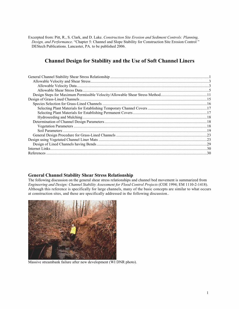
General Channel Stability Shear Stress Relationship The following discussion on the general shear stress relationships and channel bed movement is summarized from

Engineering and Design: Channel Stability Assessment for Flood Control Projects (COE 1994; EM 1110-2-1418).

Although this reference is specifically for large channels, many of the basic concepts are similar to what occurs

at construction sites, and these are specifically addressed in the following discussion..

Massive streambank failure after new development (WI DNR photo).

2

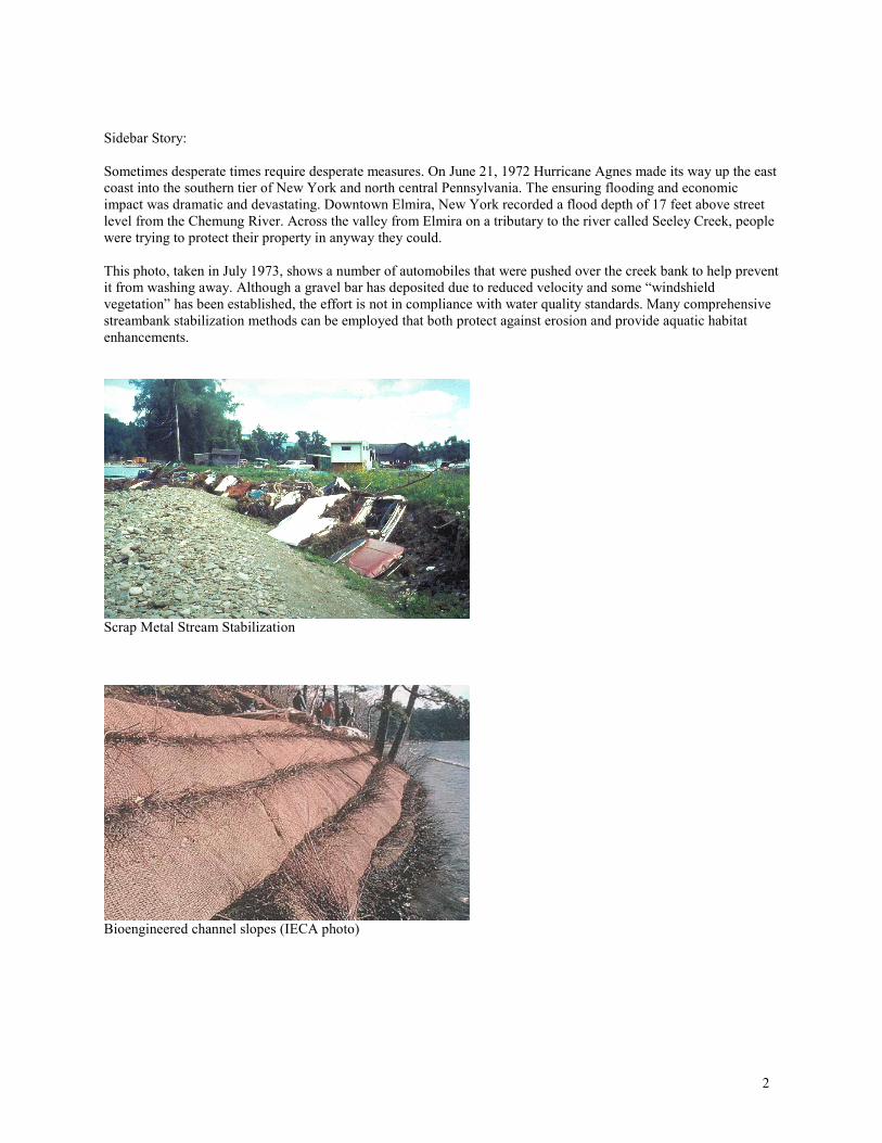
Sidebar Story:

Sometimes desperate times require desperate measures. On June 21, 1972 Hurricane Agnes made its way up the east

coast into the southern tier of New York and north central Pennsylvania. The ensuring flooding and economic

impact was dramatic and devastating. Downtown Elmira, New York recorded a flood depth of 17 feet above street

level from the Chemung River. Across the valley from Elmira on a tributary to the river called Seeley Creek, people

were trying to protect their property in anyway they could.

This photo, taken in July 1973, shows a number of automobiles that were pushed over the creek bank to help prevent

it from washing away. Although a gravel bar has deposited due to reduced velocity and some “windshield

vegetation” has been established, the effort is not in compliance with water quality standards. Many comprehensive

streambank stabilization methods can be employed that both protect against erosion and provide aquatic habitat

enhancements.

Scrap Metal Stream Stabilization

Bioengineered channel slopes (IECA photo)

3

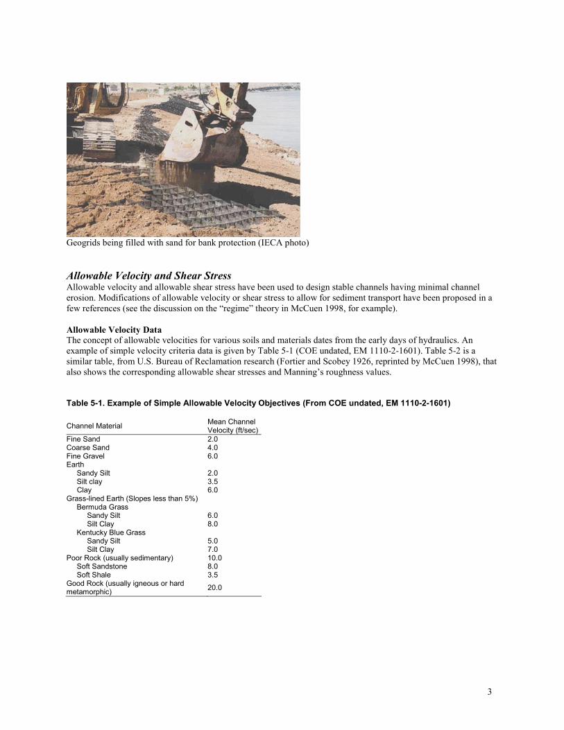
Geogrids being filled with sand for bank protection (IECA photo)

Allowable Velocity and Shear Stress Allowable velocity and allowable shear stress have been used to design stable channels having minimal channel

erosion. Modifications of allowable velocity or shear stress to allow for sediment transport have been proposed in a

few references (see the discussion on the “regime” theory in McCuen 1998, for example).

Allowable Velocity Data

The concept of allowable velocities for various soils and materials dates from the early days of hydraulics. An

example of simple velocity criteria data is given by Table 5-1 (COE undated, EM 1110-2-1601). Table 5-2 is a

similar table, from U.S. Bureau of Reclamation research (Fortier and Scobey 1926, reprinted by McCuen 1998), that

also shows the corresponding allowable shear stresses and Manning’s roughness values.

Table 5-1. Example of Simple Allowable Velocity Objectives (From COE undated, EM 1110-2-1601)

Channel Material Mean Channel Velocity (ft/sec)

Fine Sand 2.0 Coarse Sand 4.0 Fine Gravel 6.0 Earth Sandy Silt 2.0 Silt clay 3.5 Clay 6.0 Grass-lined Earth (Slopes less than 5%) Bermuda Grass Sandy Silt 6.0 Silt Clay 8.0 Kentucky Blue Grass Sandy Silt 5.0 Silt Clay 7.0 Poor Rock (usually sedimentary) 10.0 Soft Sandstone 8.0 Soft Shale 3.5 Good Rock (usually igneous or hard metamorphic)

20.0

4

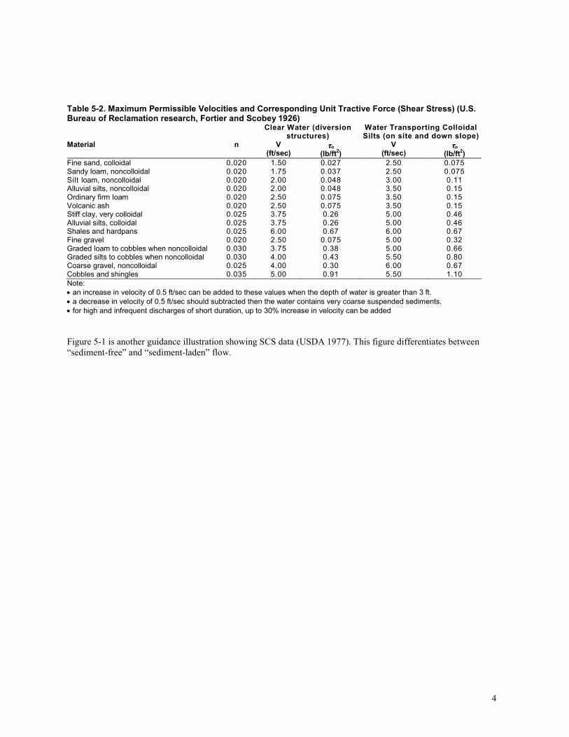
Table 5-2. Maximum Permissible Velocities and Corresponding Unit Tractive Force (Shear Stress) (U.S. Bureau of Reclamation research, Fortier and Scobey 1926)

Clear Water (diversion structures)

Water Transporting Colloidal Silts (on site and down slope)

Material n V (ft/sec)

ττττo (lb/ft

2)

V (ft/sec)

ττττo (lb/ft

2)

Fine sand, colloidal 0.020 1.50 0.027 2.50 0.075 Sandy loam, noncolloidal 0.020 1.75 0.037 2.50 0.075 Silt loam, noncolloidal 0.020 2.00 0.048 3.00 0.11 Alluvial silts, noncolloidal 0.020 2.00 0.048 3.50 0.15 Ordinary firm loam 0.020 2.50 0.075 3.50 0.15 Volcanic ash 0.020 2.50 0.075 3.50 0.15 Stiff clay, very colloidal 0.025 3.75 0.26 5.00 0.46 Alluvial silts, colloidal 0.025 3.75 0.26 5.00 0.46 Shales and hardpans 0.025 6.00 0.67 6.00 0.67 Fine gravel 0.020 2.50 0.075 5.00 0.32 Graded loam to cobbles when noncolloidal 0.030 3.75 0.38 5.00 0.66 Graded silts to cobbles when noncolloidal 0.030 4.00 0.43 5.50 0.80 Coarse gravel, noncolloidal 0.025 4.00 0.30 6.00 0.67 Cobbles and shingles 0.035 5.00 0.91 5.50 1.10

Note:

• an increase in velocity of 0.5 ft/sec can be added to these values when the depth of water is greater than 3 ft. • a decrease in velocity of 0.5 ft/sec should subtracted then the water contains very coarse suspended sediments.

• for high and infrequent discharges of short duration, up to 30% increase in velocity can be added

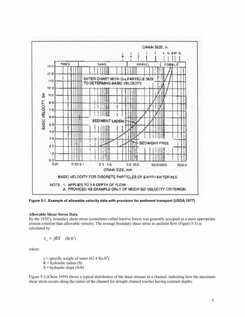
Figure 5-1 is another guidance illustration showing SCS data (USDA 1977). This figure differentiates between

“sediment-free” and “sediment-laden” flow.

5

Figure 5-1. Example of allowable velocity data with provision for sediment transport (USDA 1977)

Allowable Shear Stress Data

By the 1930’s, boundary shear stress (sometimes called tractive force) was generally accepted as a more appropriate

erosion criterion than allowable velocity. The average boundary shear stress in uniform flow (Figure 5-3) is

calculated by

RSo γτ = (lb/ft2)

where:

γ = specific weight of water (62.4 lbs/ft3)

R = hydraulic radius (ft)

S = hydraulic slope (ft/ft)

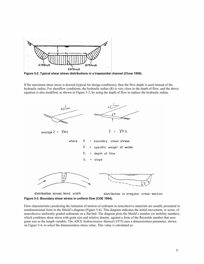
Figure 5-2 (Chow 1959) shows a typical distribution of the shear stresses in a channel, indicating how the maximum

shear stress occurs along the center of the channel for straight channel reaches having constant depths.

6

Figure 5-2. Typical shear stress distributions in a trapezoidal channel (Chow 1959).

If the maximum shear stress is desired (typical for design conditions), then the flow depth is used instead of the

hydraulic radius. For sheetflow conditions, the hydraulic radius (R) is very close to the depth of flow, and the above

equation is also modified, as shown in Figure 5-3, by using the depth of flow to replace the hydraulic radius.

Figure 5-3. Boundary shear stress in uniform flow (COE 1994).

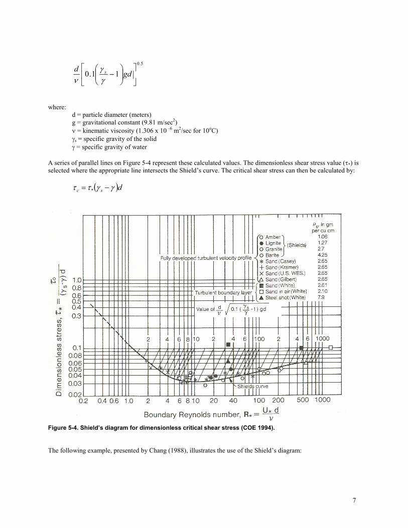
Flow characteristics predicting the initiation of motion of sediment in noncohesive materials are usually presented in

nondimensional form in the Shield’s diagram (Figure 5-4). This diagram indicates the initial movement, or scour, of

noncohesive uniformly graded sediments on a flat bed. The diagram plots the Shield’s number (or mobility number),

which combines shear stress with grain size and relative density, against a form of the Reynolds number that uses

grain size as the length variable. The ASCE Sedimentation Manual (1975) uses a dimensionless parameter, shown

on Figure 5-4, to select the dimensionless stress value. This value is calculated as:

7

5.0

11.0

− gd

d s

γγ

ν

where:

d = particle diameter (meters)

g = gravitational constant (9.81 m/sec2)

ν = kinematic viscosity (1.306 x 10 –6 m

2/sec for 10

oC)

γs = specific gravity of the solid γ = specific gravity of water

A series of parallel lines on Figure 5-4 represent these calculated values. The dimensionless shear stress value (τ*) is selected where the appropriate line intersects the Shield’s curve. The critical shear stress can then be calculated by:

( )dsc γγττ −= *

Figure 5-4. Shield’s diagram for dimensionless critical shear stress (COE 1994).

The following example, presented by Chang (1988), illustrates the use of the Shield’s diagram:

8

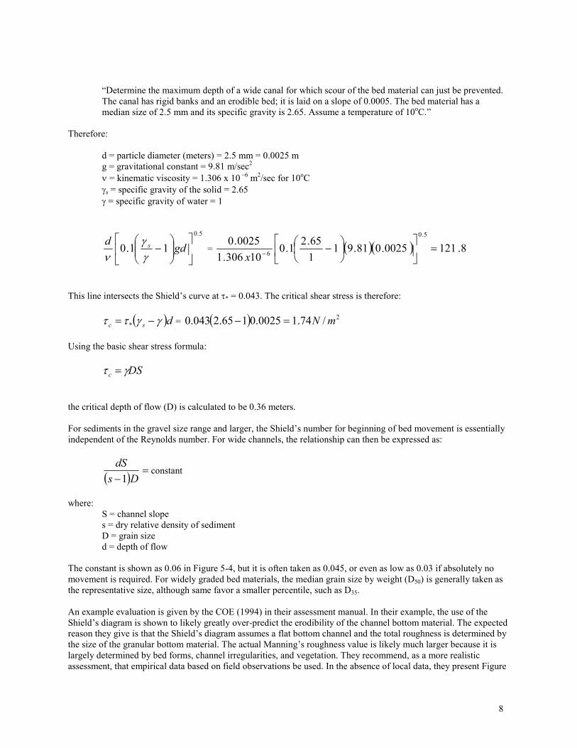
“Determine the maximum depth of a wide canal for which scour of the bed material can just be prevented.

The canal has rigid banks and an erodible bed; it is laid on a slope of 0.0005. The bed material has a

median size of 2.5 mm and its specific gravity is 2.65. Assume a temperature of 10oC.”

Therefore:

d = particle diameter (meters) = 2.5 mm = 0.0025 m

g = gravitational constant = 9.81 m/sec2

ν = kinematic viscosity = 1.306 x 10 –6 m

2/sec for 10

oC

γs = specific gravity of the solid = 2.65 γ = specific gravity of water = 1

5.0

11.0

− gd

d s

γγ

ν = ( )( ) 8.1210025.081.91

1

65.21.0

10306.1

0025.05.0

6=

−−x

This line intersects the Shield’s curve at τ* = 0.043. The critical shear stress is therefore:

( )dsc γγττ −= * = ( ) 2/74.10025.0165.2043.0 mN=−

Using the basic shear stress formula:

DSc γτ =

the critical depth of flow (D) is calculated to be 0.36 meters.

For sediments in the gravel size range and larger, the Shield’s number for beginning of bed movement is essentially

independent of the Reynolds number. For wide channels, the relationship can then be expressed as:

( )

=− Ds

dS

1constant

where:

S = channel slope

s = dry relative density of sediment

D = grain size

d = depth of flow

The constant is shown as 0.06 in Figure 5-4, but it is often taken as 0.045, or even as low as 0.03 if absolutely no

movement is required. For widely graded bed materials, the median grain size by weight (D50) is generally taken as

the representative size, although same favor a smaller percentile, such as D35.

An example evaluation is given by the COE (1994) in their assessment manual. In their example, the use of the

Shield’s diagram is shown to likely greatly over-predict the erodibility of the channel bottom material. The expected

reason they give is that the Shield’s diagram assumes a flat bottom channel and the total roughness is determined by

the size of the granular bottom material. The actual Manning’s roughness value is likely much larger because it is

largely determined by bed forms, channel irregularities, and vegetation. They recommend, as a more realistic

assessment, that empirical data based on field observations be used. In the absence of local data, they present Figure

9

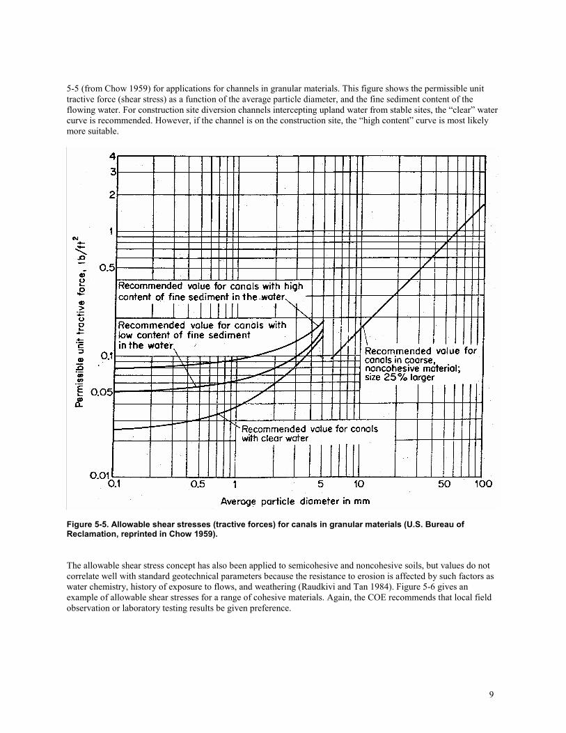
5-5 (from Chow 1959) for applications for channels in granular materials. This figure shows the permissible unit

tractive force (shear stress) as a function of the average particle diameter, and the fine sediment content of the

flowing water. For construction site diversion channels intercepting upland water from stable sites, the “clear” water

curve is recommended. However, if the channel is on the construction site, the “high content” curve is most likely

more suitable.

Figure 5-5. Allowable shear stresses (tractive forces) for canals in granular materials (U.S. Bureau of Reclamation, reprinted in Chow 1959).

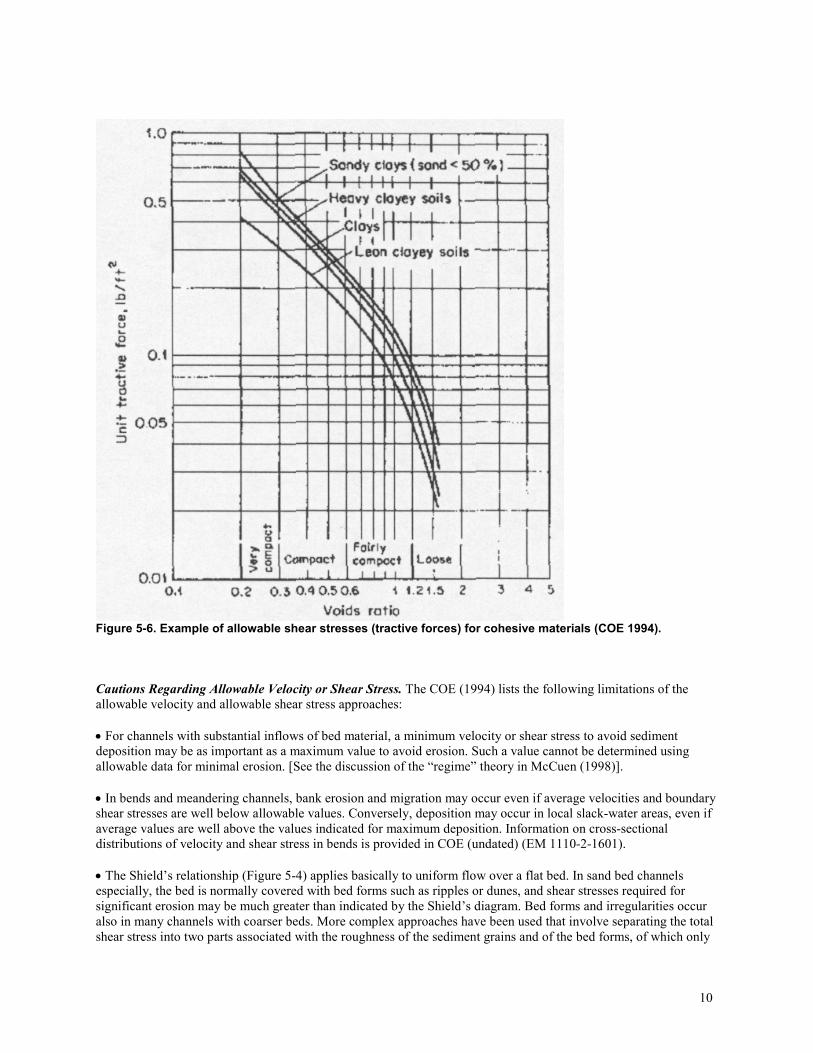
The allowable shear stress concept has also been applied to semicohesive and noncohesive soils, but values do not

correlate well with standard geotechnical parameters because the resistance to erosion is affected by such factors as

water chemistry, history of exposure to flows, and weathering (Raudkivi and Tan 1984). Figure 5-6 gives an

example of allowable shear stresses for a range of cohesive materials. Again, the COE recommends that local field

observation or laboratory testing results be given preference.

10

Figure 5-6. Example of allowable shear stresses (tractive forces) for cohesive materials (COE 1994).

Cautions Regarding Allowable Velocity or Shear Stress. The COE (1994) lists the following limitations of the

allowable velocity and allowable shear stress approaches:

• For channels with substantial inflows of bed material, a minimum velocity or shear stress to avoid sediment

deposition may be as important as a maximum value to avoid erosion. Such a value cannot be determined using

allowable data for minimal erosion. [See the discussion of the “regime” theory in McCuen (1998)].

• In bends and meandering channels, bank erosion and migration may occur even if average velocities and boundary

shear stresses are well below allowable values. Conversely, deposition may occur in local slack-water areas, even if

average values are well above the values indicated for maximum deposition. Information on cross-sectional

distributions of velocity and shear stress in bends is provided in COE (undated) (EM 1110-2-1601).

• The Shield’s relationship (Figure 5-4) applies basically to uniform flow over a flat bed. In sand bed channels

especially, the bed is normally covered with bed forms such as ripples or dunes, and shear stresses required for

significant erosion may be much greater than indicated by the Shield’s diagram. Bed forms and irregularities occur

also in many channels with coarser beds. More complex approaches have been used that involve separating the total

shear stress into two parts associated with the roughness of the sediment grains and of the bed forms, of which only

11

the first part contributes to erosion. In general, however, the Shield’s approach is not very useful for the design of

channels in fine-grained materials.

Guidelines for Applications. The following guidelines are suggested by the COE (1994) for computations and

procedures using allowable velocity and shear stress concepts:

• If cross sections and slope are reasonably uniform, computations can be based on an average section. Otherwise,

divide the project length into reaches and consider values for small, medium, and large sections.

• Determine the discharge that would cause the initiation of erosion from the stage-velocity or discharge-velocity

curve, and determine its frequency from a flood-frequency or flow-duration curve. This may give some indication of

the potential for instability. For example, if bed movement has a return period measured in years, which is the case

with some cobble or boulder channels, the potential for extensive profile instability is likely to be negligible. On the

other hand, if the bed is evidently active at relatively frequent flows, response to channel modifications may be rapid

and extensive.

Design Steps for Maximum Permissible Velocity/Allowable Shear Stress Method McCuen (1998) presents the following steps when designing a stable channel using the permissible

velocity/allowable shear stress method:

1) for a given channel material, estimate the Manning’s roughness coefficient (n), the channel slope (S), and the

maximum permissible velocity (V) (such as from Tables 5-1 or 5-2).

2) Compute the hydraulic radius (R) using Manning’s equation:

5.1

5.049.1

=S

VnR

where:

R = hydraulic radius, ft.

V = permissible velocity, ft/sec

S = channel slope, ft/ft

n = roughness of channel lining material, dimensionless

Some typical values for Manning’s n for open channels (Chow 1959) are as follows:

Very smooth surface (glass, plastic, machined metal) 0.010

Planed timber 0.011

Rough wood 0.012 – 0.015

Smooth concrete 0.012 – 0.013

Unfinished concrete 0.013 – 0.016

Brickwork 0.014

Rubble masonry 0.017

Earth channels, smooth no weeds 0.020

Firm gravel 0.020

Earth channel, with some stones and weeds 0.025

Earth channels in bad condition, winding natural streams 0.035

Mountain streams 0.040 – 0.050

Sand (flat bed), or gravel channels, d=median grain diameter, ft. 0.034d1/6

Chow (1959) also provides an extensive list of n values, along with photographs. All engineering hydrology texts

(including McCuen 1998) will also contain extensive guidance on the selection of Manning’s n values.

12

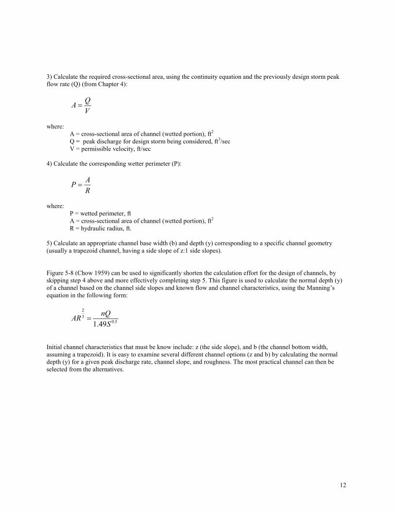
3) Calculate the required cross-sectional area, using the continuity equation and the previously design storm peak

flow rate (Q) (from Chapter 4):

V

QA =

where:

A = cross-sectional area of channel (wetted portion), ft2

Q = peak discharge for design storm being considered, ft3/sec

V = permissible velocity, ft/sec

4) Calculate the corresponding wetter perimeter (P):

R

AP =

where:

P = wetted perimeter, ft

A = cross-sectional area of channel (wetted portion), ft2

R = hydraulic radius, ft.

5) Calculate an appropriate channel base width (b) and depth (y) corresponding to a specific channel geometry

(usually a trapezoid channel, having a side slope of z:1 side slopes).

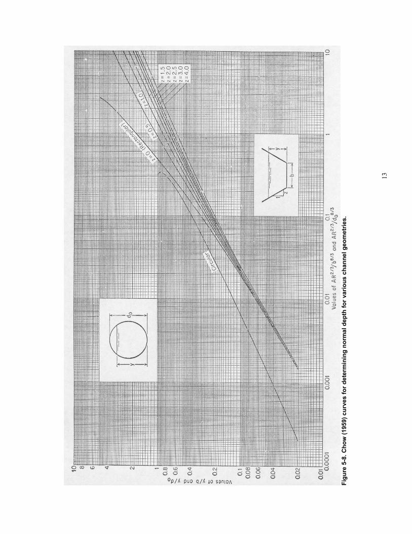
Figure 5-8 (Chow 1959) can be used to significantly shorten the calculation effort for the design of channels, by

skipping step 4 above and more effectively completing step 5. This figure is used to calculate the normal depth (y)

of a channel based on the channel side slopes and known flow and channel characteristics, using the Manning’s

equation in the following form:

5.0

3

2

49.1 S

nQAR =

Initial channel characteristics that must be know include: z (the side slope), and b (the channel bottom width,

assuming a trapezoid). It is easy to examine several different channel options (z and b) by calculating the normal

depth (y) for a given peak discharge rate, channel slope, and roughness. The most practical channel can then be

selected from the alternatives.

13

Figure 5-8. Chow (1959) curves for determining normal depth for various channel geometries.

14

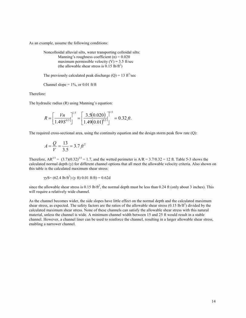
As an example, assume the following conditions:

Noncolloidal alluvial silts, water transporting colloidal silts:

Manning’s roughness coefficient (n) = 0.020

maximum permissible velocity (V) = 3.5 ft/sec

(the allowable shear stress is 0.15 lb/ft2)

The previously calculated peak discharge (Q) = 13 ft3/sec

Channel slope = 1%, or 0.01 ft/ft

Therefore:

The hydraulic radius (R) using Manning’s equation:

5.1

5.049.1

=S

VnR

( )( )

.32.001.049.1

020.05.35.1

5.0ft=

=

The required cross-sectional area, using the continuity equation and the design storm peak flow rate (Q):

V

QA = 27.3

5.3

13ft==

Therefore, AR2/3 = (3.7)(0.32)

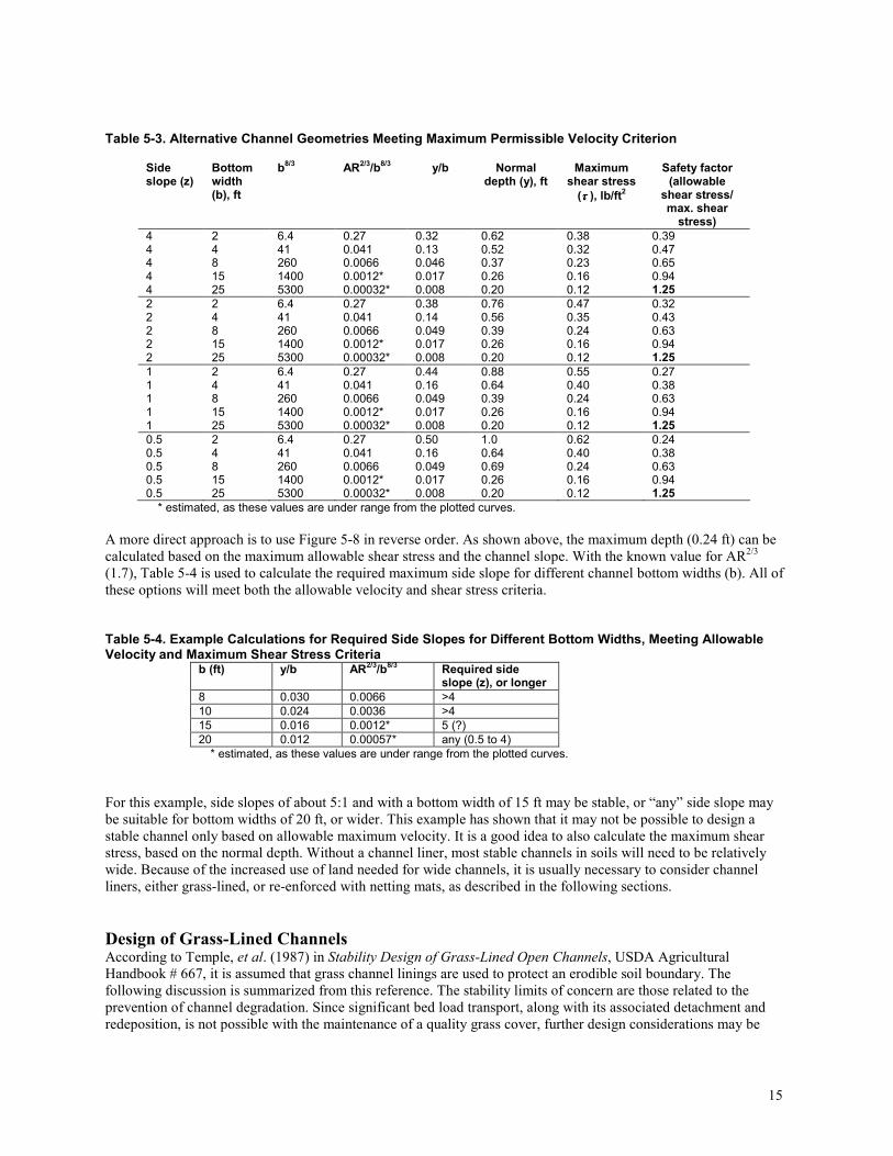
2/3 = 1.7, and the wetted perimeter is A/R = 3.7/0.32 = 12 ft. Table 5-3 shows the

calculated normal depth (y) for different channel options that all meet the allowable velocity criteria. Also shown on

this table is the calculated maximum shear stress:

γyS= (62.4 lb/ft3) (y ft) 0.01 ft/ft) = 0.62d

since the allowable shear stress is 0.15 lb/ft2, the normal depth must be less than 0.24 ft (only about 3 inches). This

will require a relatively wide channel.

As the channel becomes wider, the side slopes have little effect on the normal depth and the calculated maximum

shear stress, as expected. The safety factors are the ratios of the allowable shear stress (0.15 lb/ft2) divided by the

calculated maximum shear stress. None of these channels can satisfy the allowable shear stress with this natural

material, unless the channel is wide. A minimum channel width between 15 and 25 ft would result in a stable

channel. However, a channel liner can be used to reinforce the channel, resulting in a larger allowable shear stress,

enabling a narrower channel.

15

Table 5-3. Alternative Channel Geometries Meeting Maximum Permissible Velocity Criterion

Side slope (z)

Bottom width (b), ft

b8/3 AR

2/3/b8/3 y/b Normal

depth (y), ft Maximum shear stress

(ττττ ), lb/ft2

Safety factor (allowable shear stress/ max. shear stress)

4 2 6.4 0.27 0.32 0.62 0.38 0.39 4 4 41 0.041 0.13 0.52 0.32 0.47 4 8 260 0.0066 0.046 0.37 0.23 0.65 4 15 1400 0.0012* 0.017 0.26 0.16 0.94 4 25 5300 0.00032* 0.008 0.20 0.12 1.25

2 2 6.4 0.27 0.38 0.76 0.47 0.32 2 4 41 0.041 0.14 0.56 0.35 0.43 2 8 260 0.0066 0.049 0.39 0.24 0.63 2 15 1400 0.0012* 0.017 0.26 0.16 0.94 2 25 5300 0.00032* 0.008 0.20 0.12 1.25

1 2 6.4 0.27 0.44 0.88 0.55 0.27 1 4 41 0.041 0.16 0.64 0.40 0.38 1 8 260 0.0066 0.049 0.39 0.24 0.63 1 15 1400 0.0012* 0.017 0.26 0.16 0.94 1 25 5300 0.00032* 0.008 0.20 0.12 1.25

0.5 2 6.4 0.27 0.50 1.0 0.62 0.24 0.5 4 41 0.041 0.16 0.64 0.40 0.38 0.5 8 260 0.0066 0.049 0.69 0.24 0.63 0.5 15 1400 0.0012* 0.017 0.26 0.16 0.94 0.5 25 5300 0.00032* 0.008 0.20 0.12 1.25

* estimated, as these values are under range from the plotted curves.

A more direct approach is to use Figure 5-8 in reverse order. As shown above, the maximum depth (0.24 ft) can be

calculated based on the maximum allowable shear stress and the channel slope. With the known value for AR2/3

(1.7), Table 5-4 is used to calculate the required maximum side slope for different channel bottom widths (b). All of

these options will meet both the allowable velocity and shear stress criteria.

Table 5-4. Example Calculations for Required Side Slopes for Different Bottom Widths, Meeting Allowable Velocity and Maximum Shear Stress Criteria

b (ft) y/b AR2/3/b8/3 Required side

slope (z), or longer

8 0.030 0.0066 >4

10 0.024 0.0036 >4

15 0.016 0.0012* 5 (?)

20 0.012 0.00057* any (0.5 to 4)

* estimated, as these values are under range from the plotted curves.

For this example, side slopes of about 5:1 and with a bottom width of 15 ft may be stable, or “any” side slope may

be suitable for bottom widths of 20 ft, or wider. This example has shown that it may not be possible to design a

stable channel only based on allowable maximum velocity. It is a good idea to also calculate the maximum shear

stress, based on the normal depth. Without a channel liner, most stable channels in soils will need to be relatively

wide. Because of the increased use of land needed for wide channels, it is usually necessary to consider channel

liners, either grass-lined, or re-enforced with netting mats, as described in the following sections.

Design of Grass-Lined Channels According to Temple, et al. (1987) in Stability Design of Grass-Lined Open Channels, USDA Agricultural

Handbook # 667, it is assumed that grass channel linings are used to protect an erodible soil boundary. The

following discussion is summarized from this reference. The stability limits of concern are those related to the

prevention of channel degradation. Since significant bed load transport, along with its associated detachment and

redeposition, is not possible with the maintenance of a quality grass cover, further design considerations may be

16

needed to limit particle or aggregate detachment processes. This limitation results in the logical dominant parameter

being the boundary stress effective in generating a tractive force on detachable particles or aggregates.

For the soils most often encountered in grass-lined channel design, particle detachment begins at levels of total

stress low enough to be withstood by the vegetation without significant damage to the plants themselves. However,

when this occurs, the vegetation is undercut and the weaker vegetation is removed. This removal decreases the

density and uniformity of the cover, which in turn leads to greater stresses at the soil-water interface, resulting in an

increased erosion rate. Supercritical flow causes a more severe problem by the tendency for slight boundary or cover

discontinuities to cause flow and stress concentrations to develop during these flow conditions.

For very erosion-resistant soils, the plants may sustain damage before the effective stress at the soil-water interface

becomes large enough to detach soil particles or aggregates. Although the limiting condition in this case is the stress

on the plants, failure progresses in a similar manner: damage to the plant cover results in an increase in effective

stress on the soil boundary until conditions critical to erosion are exceeded. The ensuing erosion further weakens the

cover, and unraveling occurs.

The potential for rapid unraveling of a channel lining once a weak point has developed, combined with the

variability of vegetative covers, requires conservative design criteria. Very dense and uniform covers may withstand

stresses substantially larger than those specified for short periods without significant damage. Reducing of the

stability limits is not advised, however, unless a high level of maintenance guarantees that an unusually dense and

uniform cover will always exist. Also, unusually poor maintenance practices or nonuniform boundary conditions

should be reflected in the design.

Because the failure most often observed in the field and in the laboratory has resulted from the weakening of the

vegetal lining by removal of soil through the lining, few data exist related to the maximum stresses that plants rooted

in highly erosion-resistant materials may withstand. Observations of cover damage under high stress conditions,

however, indicate that this type of failure may become dominant when the vegetation is established on highly

erosion-resistant soils. These observations also indicate that when plant failure occurs, it is a complex process

involving removing young and weak plants, shredding and tearing of leaves, and fatigue weakening of stems. The

use of an approximate design approach is considered appropriate for most practical applications.

Species Selection for Grass-Lined Channels This following discussion is summarized from Temple, et al. (1987). This is a general discussion and does not

provide site-specific guidance for different climatic regions. However, it does describe the general problems

associated with establishing plants in a channel environment. Local guidance (such as from local USDA or

University Extension services) needs to be sought for specific recommendations for a specific location.

The selection of grass species for use in channels is based on site-specific factors: (1) soil texture, (2) depth of

underlying material, (3) management requirements of vegetation, (4) climate, (5) slope, and (6) type of structure or

engineering design. Expected flow rate, availability of seed, ease of stand establishment (germination and seedling

growth habit), species or vegetative growth habit, plant cover (aerial parts, height, and mulch), and persistence of

established species, are other factors that must be considered in selecting the appropriate grass to meet conditions

critical to channel stability.

Soil and climate of a particular area determine the best adapted grass species for erosion control in lined channels:

1) Sandy soils take water rapidly, but do not retain moisture as long as finer textured soils.

2) Moisture is more readily caught, stored, and returned to plants grown on sandy soils.

3) Fine-textured soils are more slowly permeable than sandy soils and are characterized by (a) greater

runoff, yet are less erodible; (b) less total storage capacity because of well-developed B horizons; and (c)

lower yield of water to plants due to the higher colloidal fraction.

Channel construction should be scheduled to allow establishment of the grass stand before subjecting the channel to

excessive flows. (Note: the use of modern channel lining systems, as discussed below, help alleviate this problem.)

17

Establishing permanent covers must be tailored for each location because channel stability is a site-specific problem

until vegetation is well established. Establishment involves liming and fertilizing, seed bed preparation, appropriate

planting dates, seeding rates, mulching, and plant-soil relationships. These activities must be properly planned, with

strict attention to rainfall patterns. Often the channel is completed too late to establish permanent grasses that grow

best during the optimum planting and establishment season. (Again, the use of available lining mats and vegetation

systems help reduce these problems.)

Selecting Plant Materials for Establishing Temporary Channel Covers

Based on flow tests on sandy clay channels, wheat (Triticum aestivum L.) is recommended for winter and sudangrass

[Sorghum sudanensis (Piper) Hitchc.] for late-summer temporary covers. These temporary covers have been shown

to increase the permissible discharge rate to five times that of an unprotected channel. Other annual and short-lived

perennials used for temporary seedings include:

• barley (Hordeum vulgare L.), noted for its early fall growth;

• oats (Avena) sativa L.), in areas of mild winters;

• mixtures of wheat, oats, barley, and rye (Secale cereale L.);

• field bromegrass (Bromus spp.); and

• ryegrasses (Lolium spp.).

Summer annuals, for example, German and foxtail millets (Setaria spp.), pearl millet [Pennisetum americanurn (L.)

Leeke], and certain cultivated sorghums other than sudangrass, may also be useful for temporary mid- to late-

summer covers. Since millets do not continue to grow as aggressively as sorghums after mowing, they may leave a

more desirable, uniformly thin mulch for the permanent seeding. Temporary seedings involve minimal cultural

treatment, short-lived but quick germinating species, and little or no maintenance. The temporary covers should be

close-drilled stands and not be allowed to go to seed. The protective cover should provide stalks, roots, and litter

into which grass seeds can be drilled the following spring or fall.

Selecting Plant Materials for Establishing Permanent Covers

Many grasses can be used for permanent vegetal channel linings. The most preferred warm- and cool-season grasses

for channels are the tight-sod-forming grasses; bermudagrass [Cyodon dactylon var dactylon (L.) Pers.], bahiagrass

(Paspalum notatum Fluggle), buffalograss [Buchloe dactyloides (Nutt.) Enge1m.], intermediate wheatgrass

[Agropyron intermedium (Host) Beauv.], Kentucky bluegrass (Poa ratensis L.), reed canarygrass (Phalaris

arundinacea L.), smooth bromegrass, (Bromus inermis Leyss.), vine mesquitegrass (Panicum obtusum H.B.K.), and

Western wheatgrass (Agropyron Smithii Rydb.). These grasses are among the most widely used species and grow

well on a variety of soils.

To understand the relation between different grasses and grass mixtures to grass-lined channel use, one must

consider growth characteristics and grass-climate compatibilities in the different geographic areas of the United

States. A grass mixture should include species adapted to the full range of soil moisture conditions on the channel

side slopes. The local NRCS and University Extension offices know the best soil-binding grass species adapted to

their particular areas and associated culture information including: seeding rates, dates of seeding particular grass

species, and cultural requirements for early maximum cover. The most important characteristic of the grasses

selected is its ability to survive and thrive in the channel environment.

Bermudagrass is probably the most widely used grass in the South. It will grow on many soil types, but at times it

may demand extra management. It forms a dense sod that persists if managed properly. When bermudagrass is used,

winter-hardy varieties should be obtained. Improved varieties, such as “Coastal,” “Midland,” “Greenfield,” “Tifton,”

and “Hardie,” do not produce seed, and must be established by sprigging. Where winters are mild, channels can be

established quickly with seed of “Arizona Common” bermudagrass. “Seed of bermudagrass,” a new seed-

propagated variety with greater winter hardiness than Arizona Common, should now be available commercially.

Bermudagrass is not shade tolerant and should not be used in mixtures containing tall grasses. However, the

inclusion of winter annual legumes such as hairy vetch (Vicia villosa Roth.), narrowleaf vetch [V. sativa L.

subspecies nigra (L.) Ehrh.], and/or a summer annual such as Korean lespedeza (Lespedeza stipulacea Maxim.) may

be beneficial to stand maintenance.

18

The selection of species used in channel establishment often depends on availability of seed or plant material.

Chronic national seed shortages of some warm-season grasses, especially seed of native species, have often led to

planting seed marginally suited to site situations. Lack of available seed of desired grass species and cultivars

adapted to specific problem sites is a major constraint often delaying or frustrating seeding programs. In addition to

the grass species or base mixture of grasses used for erosion control, carefully selected special-use plants may be

added for a specific purpose or situation. Desirable wildlife food plants may be included in the mixture if they do not

compete to the detriment of the base grasses used for erosion control. Locally adapted legumes are often added if

they are compatible with the grasses and noncompetitive. Additional information on establishment and maintenance

of grass-lined channels is provided in Temple, et al, (1987).

Hydroseeding and Mulching

Hydroseeding and mulching provide a method of planting on moderate to steep slopes, but require large amounts of

water. Mulches include:

(1) Long-stem wheat straw (preferred), clean prairie hay, and so forth. Straw or hay mulches are either broadcast and

“punched” in (4 to 5 inches deep) on moderate slopes with a straight disk, or broadcast along with an adhesive or

tacking agent on steep slopes. About 1.0 to 1.5 tons/acre of straw is desired. Mulches conserve surface moisture and

reduce summer soil surface temperatures and crusting. The disadvantages of hay and straw mulches are that they can

be a source of weed seed, and too much surface mulch, regardless of the type, can cause seedling disease problems.

Commercial wood fiber mulch materials are available for relatively level areas.

2) Soil retention blankets, or mats, made of various interlocking fabrics and plastic webbing can be used on

moderate to steep slopes in areas with a high potential for runoff. These erosion blankets prevent seeds from being

washed out by rain, and at the same time mulch and enhance germination and establishment.

Determination of Channel Design Parameters The conditions governing the stability of a grass-lined open channel are the channel geometry and slope, the

erodibility of the soil boundary, and the properties of the grass lining that relate to flow retardance potential and

boundary protection.

Vegetation Parameters

Stability design of a grass-lined open channel by considering the effective stress imposed on the soil layer requires

the determination of two vegetation parameters. The first is the retardance curve index (CI) which describes the

potential of the vegetal cover to develop flow resistance. The second is the vegetation cover factor (Cf) which

describes the degree to which the vegetation cover prevents high velocities and stresses at the soil-water interface.

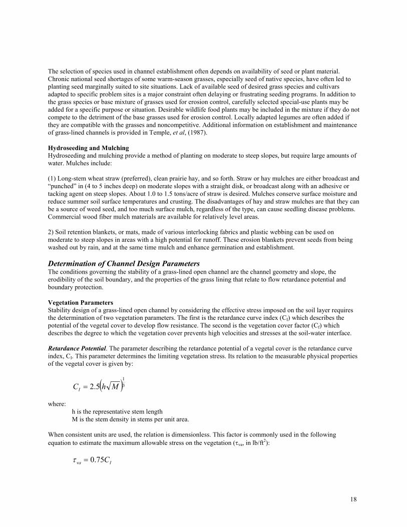
Retardance Potential. The parameter describing the retardance potential of a vegetal cover is the retardance curve

index, CI. This parameter determines the limiting vegetation stress. Its relation to the measurable physical properties

of the vegetal cover is given by:

( )31

5.2 MhCI =

where:

h is the representative stem length

M is the stem density in stems per unit area.

When consistent units are used, the relation is dimensionless. This factor is commonly used in the following

equation to estimate the maximum allowable stress on the vegetation (τva, in lb/ft2):

Iva C75.0=τ

19

The stem length will usually need to be estimated directly from knowledge of the vegetation conditions at the time

of anticipated maximum flow. When two or more grasses with widely differing growth characteristics are involved,

the representative stem length is determined as the root mean square of the individual stem lengths.

When this equation is used to estimate the retardance potential, an estimate of the stem density is also required. The

reference stem densities contained later in Table 5-5 may be used as a guide in estimating this parameter. The values

of reference stem density contained in this table were obtained from a review of the available qualitative

descriptions and stem counts reported by researchers studying channel resistance and stability.

Since cover conditions will vary from year to year and season to season, establishing an upper and a lower bound for

the curve index (CI) is often more realistic than selecting a single value. When this approach is taken, the lower

bound should be used in stability computations and the upper bound should be used in determining channel capacity.

Such an approach will normally result in satisfactory operation for lining conditions between the specified bounds.

Whatever the approach used to obtain the flow retardance potential of the lining, the values selected should

represent an average for the channel reach in question, since it will be used to infer an average energy loss per unit

of boundary area for any given flow.

Vegetation Cover Factor. The vegetation cover factor, Cf, is used to describe the degree to which the vegetation

cover prevents high velocities and stresses at the soil-water interface. Because the protective action described by this

parameter is associated with the prevention of local erosion damage which may lead to channel unraveling, the

cover factor should represent the weakest area in a reach rather than an average for the cover.

Observation of flow behavior and available data indicate that the cover factor is dominated by the density and

uniformity of density in the immediate vicinity of the soil boundary. For relatively dense and uniform covers,

uniformity of density is primarily dependent on the growth characteristics of the cover, which are in turn related to

grass type. This relationship was used in the development of Table 5-5. This table can not obviously account for

such considerations as maintenance practices or uniformity of soil fertility or moisture.

Soil Parameters

Two soil parameters are required for application of effective stress concepts to the stability design of lined or

unlined channels having an erodible soil boundary: soil grain roughness (ns) and allowable effective stress (τa). When the effective stress approach is used, the soil parameters are the same for both lined and unlined channels,

satisfying sediment transport restrictions. The relations presented here are taken from the SCS (1977) channel

stability criteria: the desired parameters, soil grain roughness and allowable stress, are determined from basic soil

parameters. Ideally, the basic parameters should be determined from tests on representative soil samples from the

site.

For effective stress design, soil grain roughness is defined as that roughness associated with particles or aggregates

of a size that may be independently moved by the flow at incipient channel failure. Although this parameter is

expressed in terms of a flow resistance coefficient (ns), its primary importance in design of vegetated channels is its

influence on effective stress, as shown below. Its contribution to the total flow resistance of a grass-lined channel is

usually negligibly small.

The allowable stress is key to the effective stress design procedure. It is defined as that stress above which an

unacceptable amount of particle or aggregate detachment would occur.

Noncohesive Soil . For purposes of determining the soil grain roughness and allowable stress, noncohesive soil is

divided into fine- or coarse-grained soil, according to the diameter for which 75 percent of the material is finer

(d75). Ideally, the point of division for hydraulic purposes would define the point at which particle submergence in

the viscous boundary layer causes pressure drag to become negligible. Strict identification of this point is

impractical for channel design applications, however. For practical application in computing soil grain roughness

and allowable effective stress, noncohesive soils are defined as fine- or coarse-grained, based on whether d75 is less

than or greater than 0.05 in. For fine-grained soils, the soil grain roughness and allowable effective stress are

20

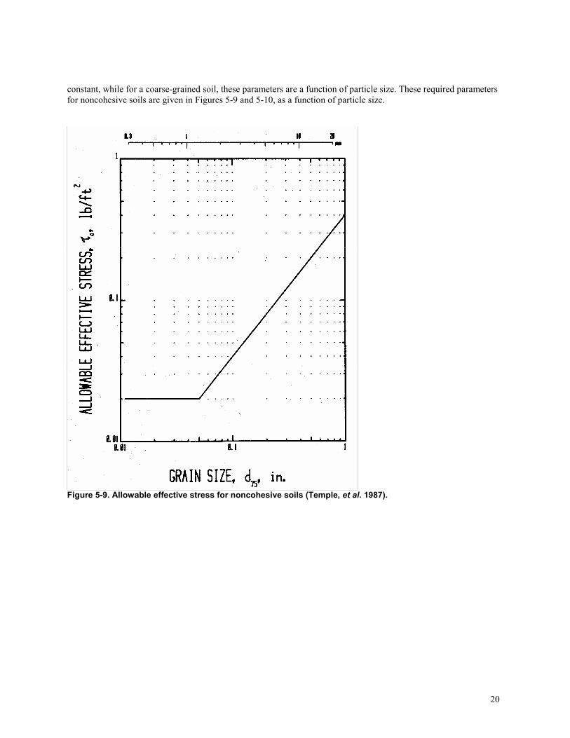
constant, while for a coarse-grained soil, these parameters are a function of particle size. These required parameters

for noncohesive soils are given in Figures 5-9 and 5-10, as a function of particle size.

Figure 5-9. Allowable effective stress for noncohesive soils (Temple, et al. 1987).

21

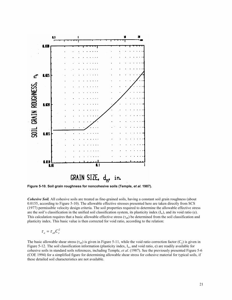
Figure 5-10. Soil grain roughness for noncohesive soils (Temple, et al. 1987).

Cohesive Soil. All cohesive soils are treated as fine-grained soils, having a constant soil grain roughness (about

0.0155, according to Figure 5-10). The allowable effective stresses presented here are taken directly from SCS

(1977) permissible velocity design criteria. The soil properties required to determine the allowable effective stress

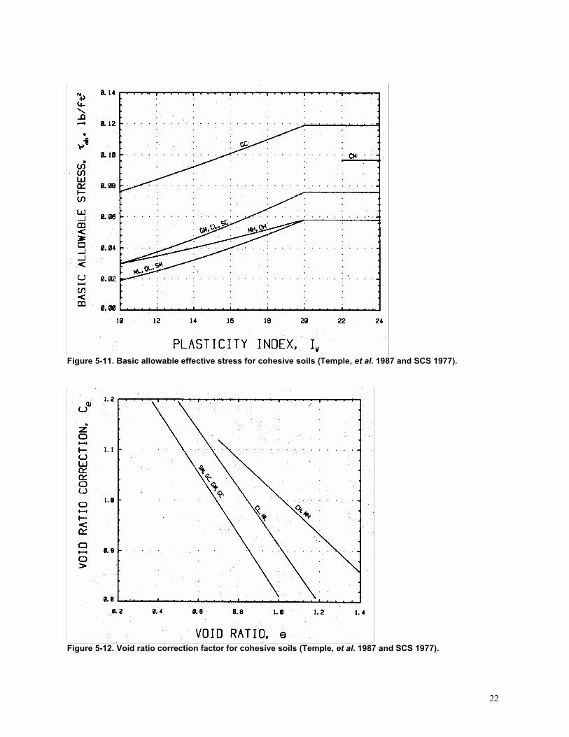
are the soil’s classification in the unified soil classification system, its plasticity index (Iw), and its void ratio (e).

This calculation requires that a basic allowable effective stress (τab) be determined from the soil classification and

plasticity index. This basic value is then corrected for void ratio, according to the relation:

2

eaba Cττ =

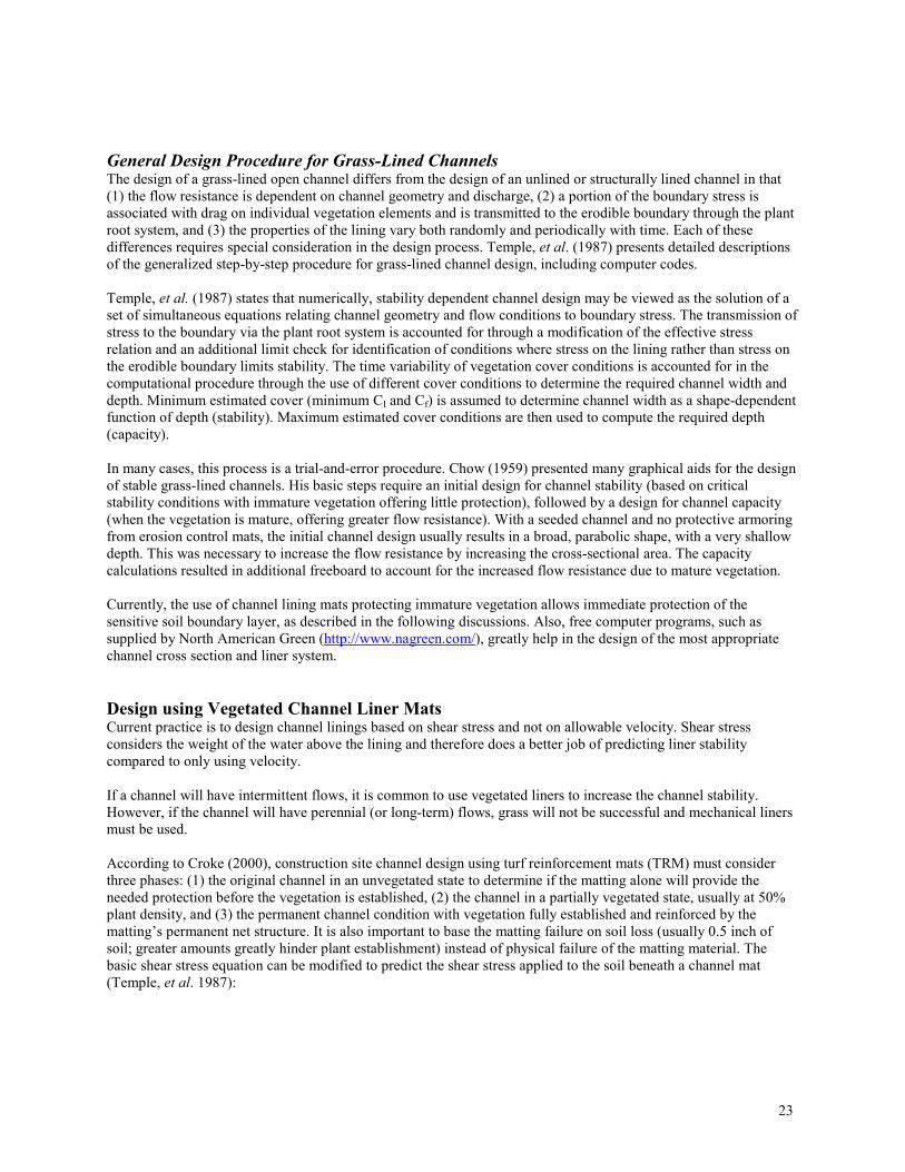
The basic allowable shear stress (τab) is given in Figure 5-11, while the void ratio correction factor (Ce) is given in

Figure 5-12. The soil classification information (plasticity index, Iw, and void ratio, e) are readily available for

cohesive soils in standard soils references, including Temple, et al. (1987). See the previously presented Figure 5-6

(COE 1994) for a simplified figure for determining allowable shear stress for cohesive material for typical soils, if

these detailed soil characteristics are not available.

22

Figure 5-11. Basic allowable effective stress for cohesive soils (Temple, et al. 1987 and SCS 1977).

Figure 5-12. Void ratio correction factor for cohesive soils (Temple, et al. 1987 and SCS 1977).

23

General Design Procedure for Grass-Lined Channels The design of a grass-lined open channel differs from the design of an unlined or structurally lined channel in that

(1) the flow resistance is dependent on channel geometry and discharge, (2) a portion of the boundary stress is

associated with drag on individual vegetation elements and is transmitted to the erodible boundary through the plant

root system, and (3) the properties of the lining vary both randomly and periodically with time. Each of these

differences requires special consideration in the design process. Temple, et al. (1987) presents detailed descriptions

of the generalized step-by-step procedure for grass-lined channel design, including computer codes.

Temple, et al. (1987) states that numerically, stability dependent channel design may be viewed as the solution of a

set of simultaneous equations relating channel geometry and flow conditions to boundary stress. The transmission of

stress to the boundary via the plant root system is accounted for through a modification of the effective stress

relation and an additional limit check for identification of conditions where stress on the lining rather than stress on

the erodible boundary limits stability. The time variability of vegetation cover conditions is accounted for in the

computational procedure through the use of different cover conditions to determine the required channel width and

depth. Minimum estimated cover (minimum CI and Cf) is assumed to determine channel width as a shape-dependent

function of depth (stability). Maximum estimated cover conditions are then used to compute the required depth

(capacity).

In many cases, this process is a trial-and-error procedure. Chow (1959) presented many graphical aids for the design

of stable grass-lined channels. His basic steps require an initial design for channel stability (based on critical

stability conditions with immature vegetation offering little protection), followed by a design for channel capacity

(when the vegetation is mature, offering greater flow resistance). With a seeded channel and no protective armoring

from erosion control mats, the initial channel design usually results in a broad, parabolic shape, with a very shallow

depth. This was necessary to increase the flow resistance by increasing the cross-sectional area. The capacity

calculations resulted in additional freeboard to account for the increased flow resistance due to mature vegetation.

Currently, the use of channel lining mats protecting immature vegetation allows immediate protection of the

sensitive soil boundary layer, as described in the following discussions. Also, free computer programs, such as

supplied by North American Green (http://www.nagreen.com/), greatly help in the design of the most appropriate

channel cross section and liner system.

Design using Vegetated Channel Liner Mats Current practice is to design channel linings based on shear stress and not on allowable velocity. Shear stress

considers the weight of the water above the lining and therefore does a better job of predicting liner stability

compared to only using velocity.

If a channel will have intermittent flows, it is common to use vegetated liners to increase the channel stability.

However, if the channel will have perennial (or long-term) flows, grass will not be successful and mechanical liners

must be used.

According to Croke (2000), construction site channel design using turf reinforcement mats (TRM) must consider

three phases: (1) the original channel in an unvegetated state to determine if the matting alone will provide the

needed protection before the vegetation is established, (2) the channel in a partially vegetated state, usually at 50%

plant density, and (3) the permanent channel condition with vegetation fully established and reinforced by the

matting’s permanent net structure. It is also important to base the matting failure on soil loss (usually 0.5 inch of

soil; greater amounts greatly hinder plant establishment) instead of physical failure of the matting material. The

basic shear stress equation can be modified to predict the shear stress applied to the soil beneath a channel mat

(Temple, et al. 1987):

24

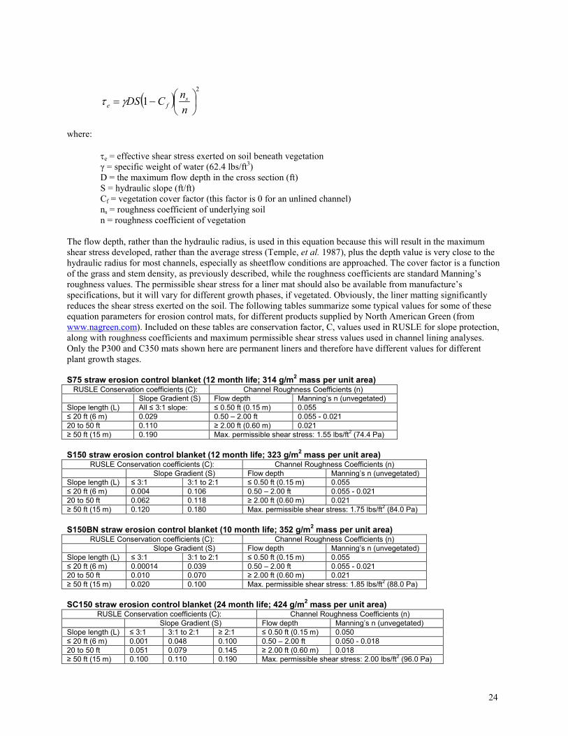
( )2

1

−=n

nCDS s

fe γτ

where:

τe = effective shear stress exerted on soil beneath vegetation γ = specific weight of water (62.4 lbs/ft

3)

D = the maximum flow depth in the cross section (ft)


Cf = vegetation cover factor (this factor is 0 for an unlined channel)

ns = roughness coefficient of underlying soil

n = roughness coefficient of vegetation

The flow depth, rather than the hydraulic radius, is used in this equation because this will result in the maximum

shear stress developed, rather than the average stress (Temple, et al. 1987), plus the depth value is very close to the

hydraulic radius for most channels, especially as sheetflow conditions are approached. The cover factor is a function

of the grass and stem density, as previously described, while the roughness coefficients are standard Manning’s

roughness values. The permissible shear stress for a liner mat should also be available from manufacture’s

specifications, but it will vary for different growth phases, if vegetated. Obviously, the liner matting significantly

reduces the shear stress exerted on the soil. The following tables summarize some typical values for some of these

equation parameters for erosion control mats, for different products supplied by North American Green (from

www.nagreen.com). Included on these tables are conservation factor, C, values used in RUSLE for slope protection,

along with roughness coefficients and maximum permissible shear stress values used in channel lining analyses.

Only the P300 and C350 mats shown here are permanent liners and therefore have different values for different

plant growth stages.

S75 straw erosion control blanket (12 month life; 314 g/m

2 mass per unit area)

RUSLE Conservation coefficients (C): Channel Roughness Coefficients (n)

Slope Gradient (S) Flow depth Manning’s n (unvegetated)

Slope length (L) All ≤ 3:1 slope: ≤ 0.50 ft (0.15 m) 0.055

≤ 20 ft (6 m) 0.029 0.50 – 2.00 ft 0.055 - 0.021

20 to 50 ft 0.110 ≥ 2.00 ft (0.60 m) 0.021

≥ 50 ft (15 m) 0.190 Max. permissible shear stress: 1.55 lbs/ft2 (74.4 Pa)

S150 straw erosion control blanket (12 month life; 323 g/m




Slope length (L) ≤ 3:1 3:1 to 2:1 ≤ 0.50 ft (0.15 m) 0.055

≤ 20 ft (6 m) 0.004 0.106 0.50 – 2.00 ft 0.055 - 0.021

20 to 50 ft 0.062 0.118 ≥ 2.00 ft (0.60 m) 0.021

≥ 50 ft (15 m) 0.120 0.180 Max. permissible shear stress: 1.75 lbs/ft2 (84.0 Pa)

S150BN straw erosion control blanket (10 month life; 352 g/m




Slope length (L) ≤ 3:1 3:1 to 2:1 ≤ 0.50 ft (0.15 m) 0.055

≤ 20 ft (6 m) 0.00014 0.039 0.50 – 2.00 ft 0.055 - 0.021

20 to 50 ft 0.010 0.070 ≥ 2.00 ft (0.60 m) 0.021

≥ 50 ft (15 m) 0.020 0.100 Max. permissible shear stress: 1.85 lbs/ft2 (88.0 Pa)

SC150 straw erosion control blanket (24 month life; 424 g/m




Slope length (L) ≤ 3:1 3:1 to 2:1 ≥ 2:1 ≤ 0.50 ft (0.15 m) 0.050

≤ 20 ft (6 m) 0.001 0.048 0.100 0.50 – 2.00 ft 0.050 - 0.018

20 to 50 ft 0.051 0.079 0.145 ≥ 2.00 ft (0.60 m) 0.018

≥ 50 ft (15 m) 0.100 0.110 0.190 Max. permissible shear stress: 2.00 lbs/ft2 (96.0 Pa)

25

SC150BN straw erosion control blanket (18 month life; 424 g/m





≤ 20 ft (6 m) 0.00009 0.029 0.063 0.50 – 2.00 ft 0.050 - 0.018

20 to 50 ft 0.005 0.055 0.092 ≥ 2.00 ft (0.60 m) 0.018

≥ 50 ft (15 m) 0.010 0.080 0.120 Max. permissible shear stress: 2.10 lbs/ft2 (100 Pa)

C125 coconut fiber erosion control blanket (36 month life; 274 g/m





≤ 20 ft (6 m) 0.001 0.029 0.082 0.50 – 2.00 ft 0.022 – 0.014

20 to 50 ft 0.036 0.060 0.096 ≥ 2.00 ft (0.60 m) 0.014


C125BN coconut fiber erosion control blanket (24 month life; 360 g/m





≤ 20 ft (6 m) 0.00009 0.018 0.050 0.50 – 2.00 ft 0.022 – 0.014

20 to 50 ft 0.003 0.040 0.060 ≥ 2.00 ft (0.60 m) 0.014


P300 polypropylene fiber erosion control blanket (permanent use; 456 g/m


RUSLE Conservation coefficients (C):

Slope Gradient (S) Channel Roughness Coefficients (n)

Slope length (L) ≤ 3:1 3:1 to 2:1 ≥ 2:1 Flow depth Manning’s n (unvegetated)

Maximum Permissible Shear Stress

≤ 20 ft (6 m) 0.001 0.029 0.082 ≤ 0.50 ft (0.15 m) 0.049 – 0.034 Unvegetated 3.00 lb/ft2 (144 Pa)

20 to 50 ft 0.036 0.060 0.096 0.50 – 2.00 ft 0.034 – 0.020 Partially vegetated 5.50 lb/ft2 (264 Pa)

≥ 50 ft (15 m) 0.070 0.090 0.110 ≥ 2.00 ft (0.60 m) 0.020 Fully vegetated 8.00 lb/ft2 (383 Pa)

Additional permissible shear stress information for vegetated North American Green products (permanent liners): Manning’s roughness coefficient (n) for flow depths: Maximum Permissible Shear Stress

Vegetated blanket type

1:

0 to 0.5 ft 0.5 to 2 ft >2 ft. Short duration (<2 hours peak flow)

Long duration (>2 hours peak flow)

C350 Phase 2 0.044 0.044 0.044 6.00 lb/ft2 (288 Pa) 4.50 lb/ft

2 (216 Pa)

P300 Phase 2 0.044 0.044 0.044 5.50 lb/ft2 (264 Pa) 4.00 lb/ft

2 (192 Pa)

C350 Phase 3 0.049 0.049 0.049 8.00 lb/ft2 (384 Pa) 8.00 lb/ft

2 (384 Pa)

P300 Phase 3 0.049 0.049 0.049 8.00 lb/ft2 (384 Pa) 8.00 lb/ft

2 (384 Pa)

1 Phase 2 is 50% stand maturity, usually at 6 months, while Phase 3 is mature growth

Values of Cf, the grass cover factor, are given in Table 5-5 (Temple, et al. 1987). They recommend multiplying the

stem densities given by 1/3, 2/3, 1, 4/3, and 5/3, for poor, fair, good, very good, and excellent covers, respectively.

Cf values for untested covers may be estimated by recognizing that the cover factor is dominated by density and

uniformity of cover near the soil surface: the sod-forming grasses near the top of the table have higher Cf values than

the bunch grasses and annuals near the bottom. For the legumes tested (alfalfa and lespedeza sericea), the effective

stem count for resistance (given on the table) is approximately five times the actual stem count very close to the bed.

Similar adjustment may be needed for other unusually large-stemmed, branching, and/ or woody vegetation.

26

Table 5-5. Properties of Grass Channel Linings (Temple, et al. 1987) Cover Factor (Cf) (good uniform stands)

Covers Tested Reference stem density (stem/ft

2)

0.90 bermudagrass 500

0.90 centipedegrass 500

0.87 buffalograss 400

0.87 kentucky bluegrass 350

0.87 blue grama 350

0.75 grass mixture 200

0.50 weeping lovegrass 350

0.50 yellow bluestem 250

0.50 alfalfa 500

0.50 lespedeza sericea 300

0.50 common lespedeza 150

0.50 sudangrass 50

As an example, consider the following conditions for a mature buffalograss on a channel liner mat:

DSo γτ = = 2.83 lb/ft2 (previously calculated), requiring a NAG P300 permanent mat, for example

ns for the soil is 0.016

n for the vegetated mat is 0.042

Cf for the vegetated mat is 0.87

The permissible shear stress for the underlying soil is 0.08 lb/ft2

Therefore:

( ) 053.0042.0

016.087.0183.2

2

=

−=eτ lb/ft2

The calculated shear stress being exerted on the soil beneath the liner mat must be less than the permissible shear

stress for the soil. In this example, the safety factor is 0.08/0.053 = 1.5 and the channel lining system is expected to

be stable.

An example of a permanent channel design and the selection of an appropriate reinforced liner is given below, based

on the simple site example in Chapter 4, Figure 4-36 and Table 4-15. The following example is for the upslope

diversion channel U2 that captures upslope runoff from 14.6 acres for diversion to an existing on-site channel. This

channel is 900 ft. long and has an 8% slope. The peak discharge was calculated to be 29 ft3/sec.

Using the Manning’s equation and the VenTe Chow (1959) shortcut on channel geometry (Figure 5-8):

5.0

3

2

49.1 S

nQAR =

Where n = 0.02

Q = 29 CFS

S = 8% (0.08)

( )( )

( )38.1

08.049.1

2902.05.0

3

2

==AR

27

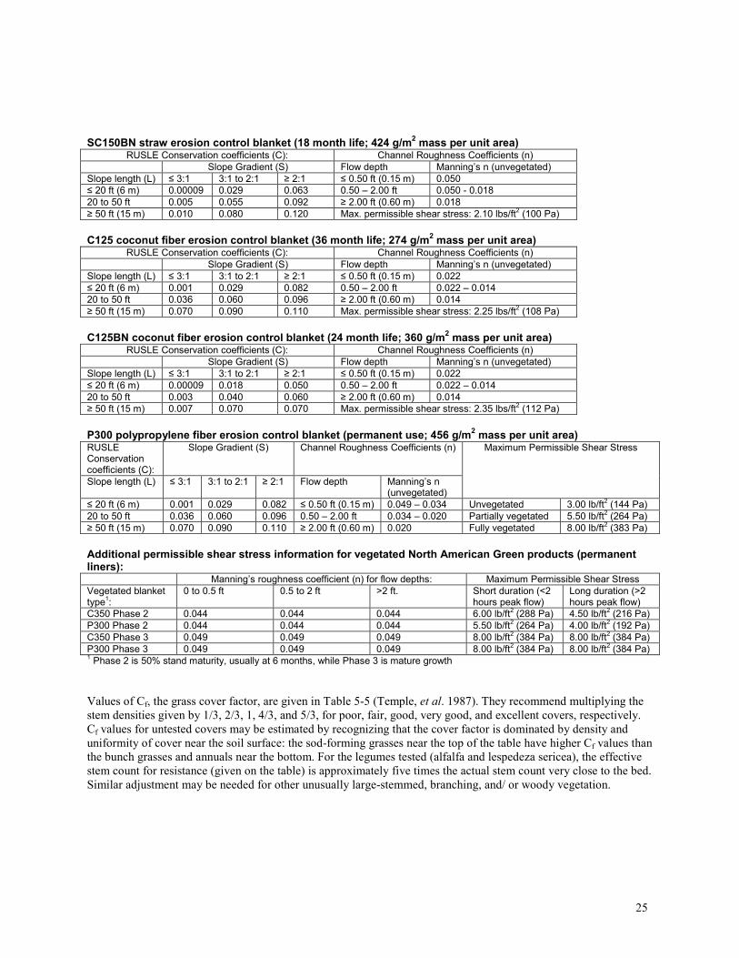
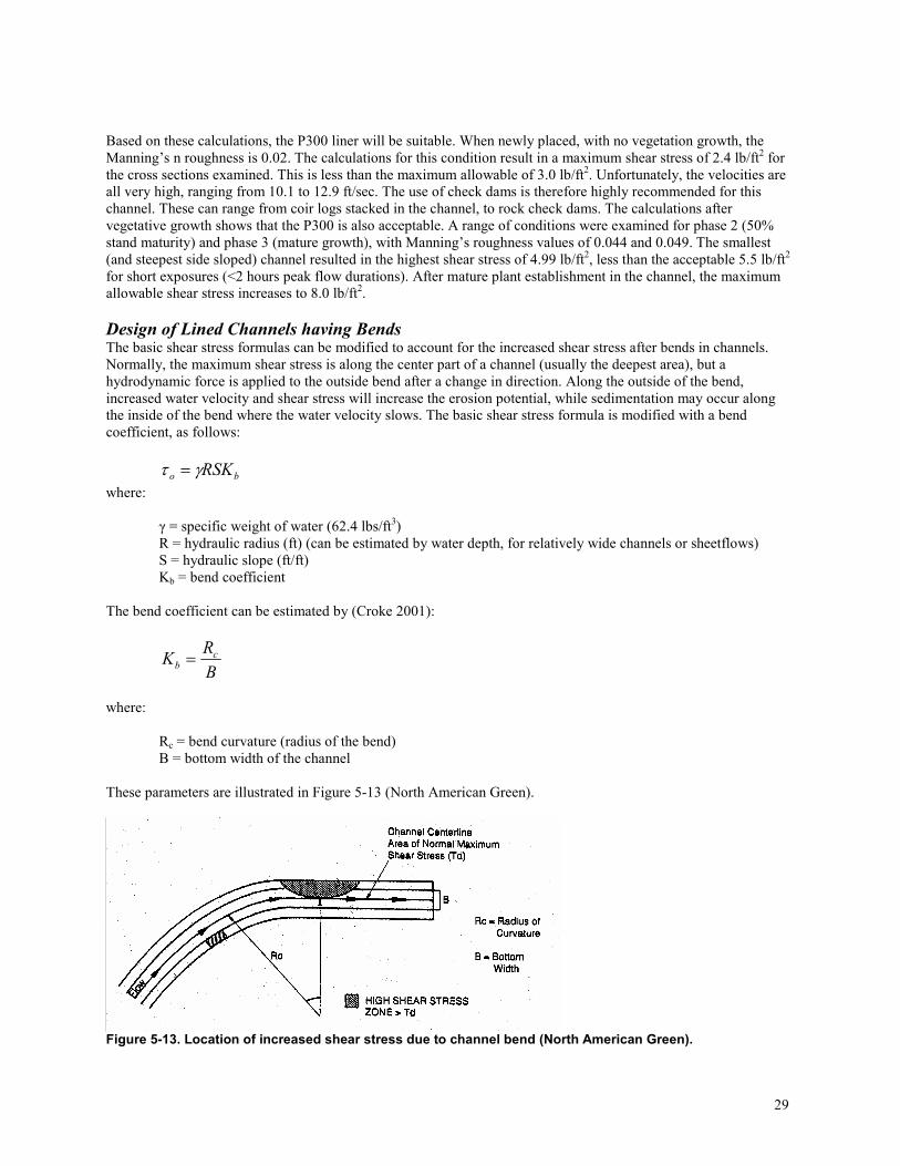
The following drawing illustrates the channel components for this basic analysis:

Figure 5-8 can be used to determine the normal depth (yn) for many combinations of bottom with (b), and side slope

(z). As an example, assume that the bottom width is 5 ft. and the side slope parameter, z, is 3. The calculated AR2/3

value (1.38) needs to be divided by b8/3 (5

8/3 = 73.14) for the shape factor used in Figure 5-8. This value is therefore:

1.38/73.14 = 0.018. For a side slope of z = 3, the figure indicates that the ratio of the depth to the bottom width (y/b)

is 0.088. In this example, the bottom width was 5 ft, so the normal depth is: yn = 0.088 (5 ft.) = 0.44 ft., which is

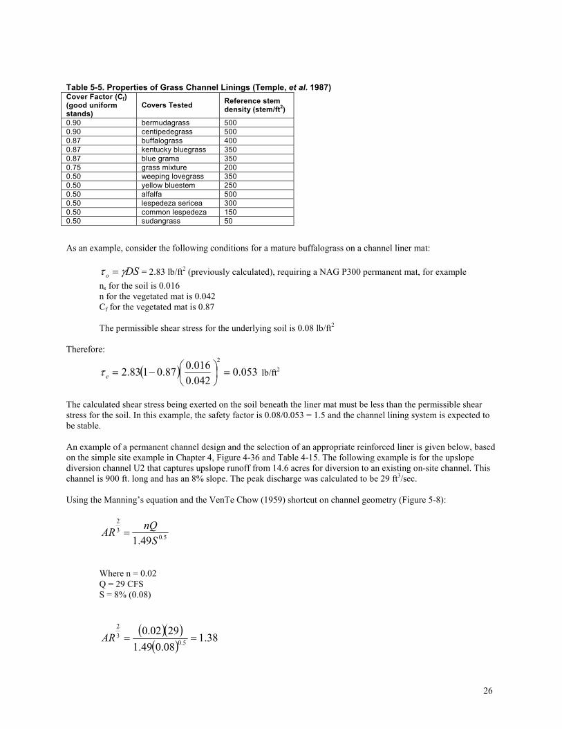
only 5.3 inches. The following shows these dimensions on the channel cross-section:

It is now possible to calculate the velocity and shear stress associated with this set of channel options:

A = [(7.64+5)/2] (0.44) = 2.78 ft2

V = Q/A = 29 ft3/sec/2.78 ft

2 = 10.4 ft/sec

R = A/P, and P = 5 + 2(3.16)(0.44) = 7.78 ft.; R = A/P = 2.78 ft2/7.78 ft. = 0.36 ft.

and τ = γRS = (62.4lb/ft3)(0.36 ft.)(0.08) = 1.8 lb/ft

2

With a velocity of 10.4 ft/sec and a shear stress of 1.8 lb/ft2, it is obvious that some type of channel reinforcement

will be needed (refer to Table 5-2), or a new design option. Using Figure 5-8, plus liner information (such as listed

previously), it is possible to create a simple spreadsheet with multiple cross section and liner options, as shown in

Table 5-6..

28

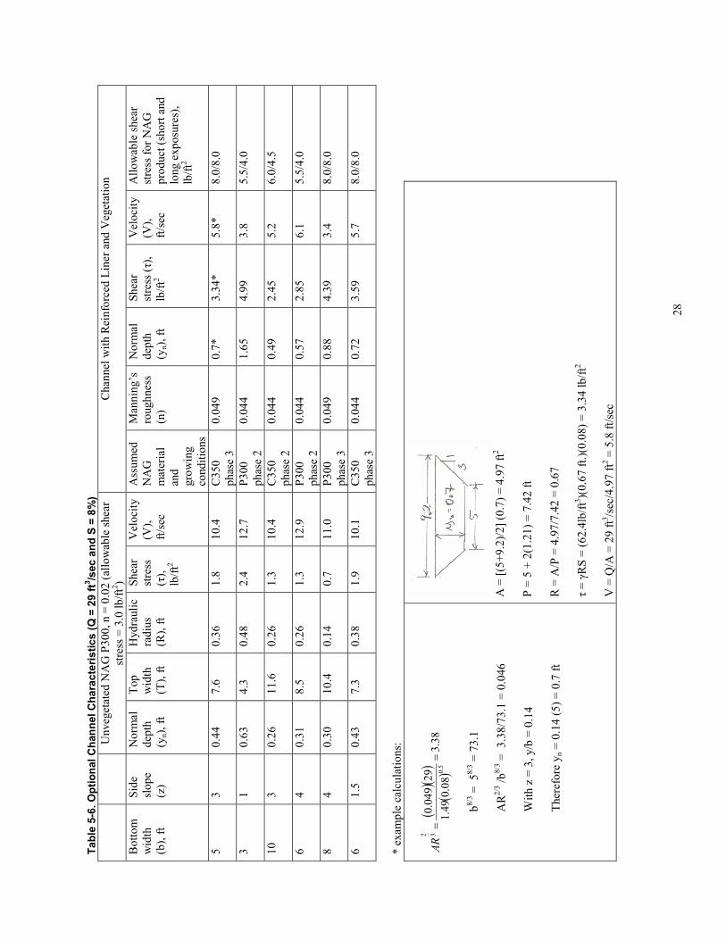
Table 5-6. Optional Channel Characteristics (Q = 29 ft3/sec and S = 8%)

Unvegetated NAG P300, n = 0.02 (allowable shear

stress = 3.0 lb/ft2)

Channel with Reinforced Liner and Vegetation

Bottom

width

(b), ft

Side

slope

(z)

Norm

al

depth

(yn), ft

Top

width

(T), ft

Hydraulic

radius

(R), ft

Shear

stress

(τ),

lb/ft2

Velocity

(V),

ft/sec

Assumed

NAG

material

and

growing

conditions

Manning’s

roughness

(n)

Norm

al

depth

(yn), ft

Shear

stress (τ),

lb/ft2

Velocity

(V),

ft/sec

Allowable shear

stress for NAG

product (short and

long exposures),

lb/ft2

5

3

0.44

7.6

0.36

1.8

10.4

C350

phase 3

0.049

0.7*

3.34*

5.8*

8.0/8.0

3

1

0.63

4.3

0.48

2.4

12.7

P300

phase 2

0.044

1.65

4.99

3.8

5.5/4.0

10

3

0.26

11.6

0.26

1.3

10.4

C350

phase 2

0.044

0.49

2.45

5.2

6.0/4.5

6

4

0.31

8.5

0.26

1.3

12.9

P300

phase 2

0.044

0.57

2.85

6.1

5.5/4.0

8

4

0.30

10.4

0.14

0.7

11.0

P300

phase 3

0.049

0.88

4.39

3.4

8.0/8.0

6

1.5

0.43

7.3

0.38

1.9

10.1

C350

phase 3

0.044

0.72

3.59

5.7

8.0/8.0

* example calculations:

()(

)(

)38

.3

08

.0

49

.1

29

049

.0

5.0

32

==

AR

b8/3 = 58/3 = 73.1

AR

2/3 /b8/3 = 3.38/73.1 = 0.046

With z = 3, y/b = 0.14

Therefore y

n = 0.14 (5) = 0.7 ft

A = [(5+9.2)/2] (0.7) = 4.97 ft2

P = 5 + 2(1.21) = 7.42 ft

R = A/P = 4.97/7.42 = 0.67

τ = γRS = (62.4lb/ft3)(0.67 ft.)(0.08) = 3.34 lb/ft2

V = Q/A = 29 ft3/sec/4.97 ft2 = 5.8 ft/sec

29

Based on these calculations, the P300 liner will be suitable. When newly placed, with no vegetation growth, the

Manning’s n roughness is 0.02. The calculations for this condition result in a maximum shear stress of 2.4 lb/ft2 for

the cross sections examined. This is less than the maximum allowable of 3.0 lb/ft2. Unfortunately, the velocities are

all very high, ranging from 10.1 to 12.9 ft/sec. The use of check dams is therefore highly recommended for this

channel. These can range from coir logs stacked in the channel, to rock check dams. The calculations after

vegetative growth shows that the P300 is also acceptable. A range of conditions were examined for phase 2 (50%

stand maturity) and phase 3 (mature growth), with Manning’s roughness values of 0.044 and 0.049. The smallest

(and steepest side sloped) channel resulted in the highest shear stress of 4.99 lb/ft2, less than the acceptable 5.5 lb/ft

2

for short exposures (<2 hours peak flow durations). After mature plant establishment in the channel, the maximum

allowable shear stress increases to 8.0 lb/ft2.

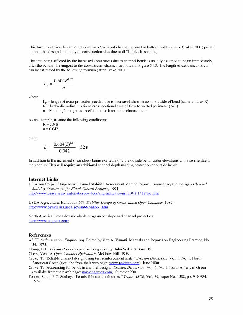
Design of Lined Channels having Bends The basic shear stress formulas can be modified to account for the increased shear stress after bends in channels.

Normally, the maximum shear stress is along the center part of a channel (usually the deepest area), but a

hydrodynamic force is applied to the outside bend after a change in direction. Along the outside of the bend,

increased water velocity and shear stress will increase the erosion potential, while sedimentation may occur along

the inside of the bend where the water velocity slows. The basic shear stress formula is modified with a bend

coefficient, as follows:

bo RSKγτ =

where:

γ = specific weight of water (62.4 lbs/ft3)

R = hydraulic radius (ft) (can be estimated by water depth, for relatively wide channels or sheetflows)


Kb = bend coefficient

The bend coefficient can be estimated by (Croke 2001):

B

RK c

b =

where:

Rc = bend curvature (radius of the bend)

B = bottom width of the channel

These parameters are illustrated in Figure 5-13 (North American Green).

Figure 5-13. Location of increased shear stress due to channel bend (North American Green).

30

This formula obviously cannot be used for a V-shaped channel, where the bottom width is zero. Croke (2001) points

out that this design is unlikely on construction sites due to difficulties in shaping.

The area being affected by the increased shear stress due to channel bends is usually assumed to begin immediately

after the bend at the tangent to the downstream channel, as shown in Figure 5-13. The length of extra shear stress

can be estimated by the following formula (after Croke 2001):

n

RLp

17.1604.0=

where:

Lp = length of extra protection needed due to increased shear stress on outside of bend (same units as R)

R = hydraulic radius = ratio of cross-sectional area of flow to wetted perimeter (A/P)

n = Manning’s roughness coefficient for liner in the channel bend

As an example, assume the following conditions:

R = 3.0 ft

n = 0.042

then:

52042.0

)3(604.0 17.1

==pL ft

In addition to the increased shear stress being exerted along the outside bend, water elevations will also rise due to

momentum. This will require an additional channel depth needing protection at outside bends.

Internet Links US Army Corps of Engineers Channel Stability Assessment Method Report: Engineering and Design - Channel

Stability Assessment for Flood Control Projects, 1994:

http://www.usace.army.mil/inet/usace-docs/eng-manuals/em1110-2-1418/toc.htm

USDA Agricultural Handbook 667: Stability Design of Grass-Lined Open Channels, 1987:

http://www.pswcrl.ars.usda.gov/ah667/ah667.htm

North America Green downloadable program for slope and channel protection:

http://www.nagreen.com/

References ASCE. Sedimentation Engineering. Edited by Vito A. Vanoni. Manuals and Reports on Engineering Practice, No.

54. 1975.

Chang, H.H. Fluvial Processes in River Engineering. John Wiley & Sons. 1988.

Chow, Ven Te. Open Channel Hydraulics. McGraw-Hill. 1959.

Croke, T. “Reliable channel design using turf reinforcement mats.” Erosion Discussion. Vol. 5, No. 1. North

American Green (availabe from their web page: www.nagreen.com). June 2000.

Croke, T. “Accounting for bends in channel design.” Erosion Discussion. Vol. 6, No. 1. North American Green

(availabe from their web page: www.nagreen.com). Summer 2001.

Fortier, S. and F.C. Scobey. “Permissible canal velocities.” Trans. ASCE, Vol. 89, paper No. 1588, pp. 940-984.

1926.

31

McCuen, R.H. Hydrologic Analysis and Design, 2nd Edition. Prentice Hall. 1998.

Raudkivi, A. J., and Tan, S. K. “Erosion of cohesive soils,” Journal of Hydraulic Research, Vol 22, No. 4, pp 217-

233. 1984.

SCS (Soil Conservation Service). Handbook for Channel Design for Soil and Water Conservation. SCS-TP-61, rev.

1954.

SCS (Soil Conservation Service). Design of Open Channels. TR-25. 1977.

U.S. Army Corps of Engineers (COE). Hydraulic Design of Flood Control Channels. EM 1110-2-1601. U.S. Army

Engineer Waterways Experiment Station, Vicksburg, MS. undated.

U.S. Army Corps of Engineers (COE). Engineering and Design: Channel Stability Assessment for Flood Control

Projects. EM 1110-2-1418. U.S. Army Engineer Waterways Experiment Station, Vicksburg, MS. 1994.

U.S. Department of Agriculture (USDA). Design of Open Channels. Technical Release No. 25, Soil

Conservation Service, Washington, DC. 1977.

USDA. Stability Design of Grass-Lined Open Channels. Agricultural Handbook 667. 1987:

Williams, D. T., and Julien, P. Y. “Examination of stage-discharge relationships of compound/composite channels,”

Proceedings of the International Conference on Channel Flow and Catchment Runoff. B.C. Yen, ed., University

of Virginia, Charlottesville, 22-26 May 1989, pp 478-488. 1989.

Documents

M6 channel stability handout