DY OF CERTAIN CLASSES OF MIXED EQUILIBRIUM PROBLEMS

DISSERTATION

TIAL FULFILMENT OF THE REQUIREMENTS hUK i HE AWARD OF THE DEGREE OF

Ma : of $!)ilc IN

TICS

By

HAIDER RIZVI

^^ .n 3 * * ,^ . a.

"?r the Supervision of

.EEM RAZA KAZMI

^ P N T OF MATHEMATICS . MUSLIM UNIVERSITY

ALIGARH (INDIA)

2009

% < * — * — ».'

DS3924

De5icdte5 To

My Lovina Parents

Dr. Kialeem Raza Kazmi ^^^^..l•(;lK A. MPIUI.. I'hi)

Reader

I'honc: (Oil) V1-57I-27()I019 I Res I •91-571-2703434 <tc!l) ^91-9411804723

)^-ni;iii. krka/nii (/ email.com

DEPARTMENT OF MATHEMATICS ALIGARH MUSLIM UNIVERSITY ALIGARH 202002, INDIA

Certificate

May 15,2009

This is to certify that this dissertation entitled "Study of Certain Classes of Mixed

Equilibrium Problems" has been written by Mr. Sliuja Haider Rizvi under my

super-vision as a partial iultilment tor the award ot the degree ot Master of Fhilosoptiy

in Maliieniaiics. He lias luifiiied liie prescribed conditions given in the siaiuies and

ordinances ot Aligarh Muslim University, Aiigarh.

DF'\' " ' :.VTTC!? (Dr. Kalecm Kaza Kazmi)

CONTENTS

Acknowledgment i Preface iii

CHAPTER 1 : PRELIMINARIES 1 17

1.1 : Introduction 1

1.2 : Variational inequalities and equilibrium problems 1-3

1.3 : Mixed equilibrium problems 3-6

1.4 : Some tools of functional analysis 6-17

CHAPTER 2 : WEINER HOPE EQUATION AND 18 30 GENERALIZED MIXED EQUILIBRIUM PROBLEMS

2.1 : Introduction 18-19

2.2 : Sensitivity analysis of general mixed equilibrium problem 19-24

2.3 : Iterative algorithm and convergence analysis 25

2.4 : Generalized mixed equilibrium problems 26-29

2.5 : Existence of solution, convergence analysis and stability 29-30

CHAPTER 3 : RESOLVENT DYNAMICAL SYSTEMS FOR 31 36

MIXED EQUILIBRIUM PROBLEMS

3.1 ; Introduction 31

3.2 : Mixed equilibrium problems and dynamical systems 32-33

3.3 : Existence and stability of unique solution of 34-36

dynamical system

CHAPTER 4 : AUXILIARY PRINCIPLE TECHNIQUES FOR 37-48

MIXED EQUILIBRIUM PROBLEMS

4.1 : Introduction 37-38

4.2 : Auxiliary problem for mixed equilibrium problem 38-39

4.3 : Viscosity method 40-42

4.4 : Auxiliary problem for generalized mixed equilibrium problems 43-45

4.5 : Algorithms and their convergence analysis 45-48

CHAPTER 5 : AUXILIARY PRINCIPLE TECHNIQUES EXT- 49-57 ENDED TO GENERALIZED MIXED SET-VALUED EQUILIBRIUM PROBLEMS

5.1 : Introduction 49-50

5.2 : Formulation of problem 50-52

5.3 : Two-step iterative algorithm 53-54

5.4 : Inertial proximal iterative algorithm 55-57

BIBLIOGRAPHY 58-65

ACKNOWLEDGMENT

All praise due to Almighty, the most beneficent and merciful, who bestowed

upon me the courage, patience and strength to embark upon this worl< and carry it

to completion.

It gives me an immense pleasure to express my deep sense of gratitude and sin­

cere thanks with warm regards and honour to my esteemed supervisor Dr. Kaleem

Raza Kazmi, Reader, Department of Mathematics, Aligarh Muslim University, Ali-

garh. I immensely owe to his erudite and scrupulous guidance, judicious criticism,

magnificent devotion and sympathetic attitude that have been instrumental in get­

ting the work completed. At this moment, it is too difficult to express in words,

my respect, admiration and thankfulness for him which are unbounded and not

transferable.

I extend my sincere thanks to Prof. H.H. Khan, Chairman, Department of

Mathematics, Aligarh MusUm University, Ahgarh, for providing me the departmen­

tal facilities whenever needed. I also express my gratefulness to all my teachers in the

department for their inspiration and encouragement which provided the continuing

impetus for this work.

I place on record my special sense of gratitude to Dr.(Mrs.) Subuhi Khan,

Reader, Department of Mathematics, Ahgarh Muslim University, Aligarh for her

constructive suggestions, continuous encouragement during the hard days of this

work. I owe my profound gratitude for her.

I express my thanks to all my seniors, especially to Dr. Zakir Husain, Dr.

Faizan Ahmad Khan for their continuous encouragement, fruitful discussions and

moral support during the course of this work.

I acknowledge my thanks to all my friends and colleagues, especially Fahad

Sikander, Malik Rashid Jamal, Salahuddin Khan, Khalid Rafat Khan, Mohd. Dil-

shad, Phool Miyan, Firdousi, Nusrat, Sabiha, Faiza, Farid and Furqan for their

constantly encouragement.

At this moment, I specially remember my parents and their devotion for me

at every step of my life and all my relatives whom I missed a lot during the course

of the work. I express my profound love to my respected brother Mr. Faiz-e-ab

Haider Rizvi and to my brother-in-law Mr. Masood Hasan Rizvi also to my sisters

Mxs. Shabih Fatima Rizvi, Mrs. Tashbih Fatima Rizvi and my cutest Niece Amber

Zehra Rizvi for their most cordial and helpful role in my academic endeavor. Their

countless blessings, deep love and affection always worked as a hidden power behind

every thing I did.

Financial support in the from oi University Research Fellowship, University

Grant Commission needs also to be acknowledged.

Last but not the least, I thank to the staff of Department of Mathematics,

Aligarh Muslim University, Aligarh, especially seminar library and office staff for

their co-operation during the course of work.

All the above cited acknowledgments belong to those who some how played a

pivotal role along with this work. I can not forget the dandy strives of my unde-

scribed mates who supported me morally and mentally.

Shuja Haider Rizvi

PREFACE

The study of mixed equilibrium problems was initiated by Moudafi and Thera [55]

in 1999. Since then various generahzations of mixed equilibrium problems have been

studied by a number of mathematicians. The mixed equilibrium problems include

the variational inequalities as well as complementarity problems, convex optimiza­

tion, Nash equilibria as special cases.

One of the most important and interesting problem in the theory of mixed

equilibrium problems is to develope the iterative methods which give efficient and

implementable algorithms for solving mixed equilibrium problems. These methods

include projection method and its variant forms, linear approximation, descent and

Newton's methods and the methods based on auxiliary principle technique.

The main objective of this work is to study a number of iterative methods for

various classes of mixed equihbrium problems.

This dissertation consists of five chapters.

In chapter 1, we give a brief introduction of variational inequalities, equilib­

rium problems and mixed equilibrium problems and give the concepts and results of

functional analysis, which are needed for the presentation of the subsequent chapters.

In chapter 2, we consider some classes of mixed equilibrium problems Studied by

Moudafi [53] and Kazmi and Khan [42] in real Hilbert space. We discuss some useful

generalizations of Yosida approximation. Further using the Wiener-Hopf equation

technique, we discuss the sensitivity analysis relying on a fixed point formulation

of the given problem. Furthermore, we discuss existence of solutions, convergence

and stability analysis of an iterative algorithm for generaUzed mixed equilibrium

problems.

In chapter 3, we consider a mixed equihbrium problem in M" and give its related

Wiener-Hopf equation and fixed point formulation. Further using this fixed point

formulation and Wiener-Hopf equation, we consider a resolvent dynamical system

ni

associated to mixed equilibrium problem and discuss its existence and stability of

solution.

In chapter 4, we consider a mixed equilibrium problem in Hilbert space and

discuss the convergence analysis of the proposed iterative method based on an algo­

rithmic approach and viscosity method in order to approximate a solution of mixed

equihbrium problem. Further we consider a generalized mixed equilibrium problem

involving non-differentiable term in Hilbert space and discuss some of its special

cases. Furthermore we discuss the existence of solution of an auxiliary problem re­

lated to generahzed mixed equihbrium problem. We also discuss the convergence

analysis of iterative algorithms based on auxiliary problems.

In chapter 5, we consider a generahzed mixed equilibrium problem in Hilbert

space and its related auxiliary problems. By using KKM-Fan's theorem and fixed

point theorem we discuss the existence of the solution for the auxiliary problems.

Further these auxiliary problems enable us to suggest and analyze two-step iterative

algorithms for finding the approximate solution for general mixed set-valued equilib­

rium problem. Furthermore, we discuss the convergence analysis of these iterative

algorithms.

At the end a fairly comprehencive list of references is presented.

IV

Chapter 1

Preliminaries

1.1. Introduction

In this chapter, we give a brief introduction of variational inequahties, equihbrium

problems and mixed equilibrium problems. Further, we review the concepts and re-

suits of functional analysis, which are needed for the presentation of the subsequent

chapters. In Section 1.2, we give a brief introduction of variational inequahties and

equihbrium problems. In Section 1.3, we give a brief introduction of mixed equihbrium

problems. In Section 1.4, we review the concepts and results which are needed for the

presentation of the subsequent chapters.

1.2. Variational Inequalities and Equilibrium Problems

A very powerful mathematical theory known as theory of variational inequalities

was initiated and studied by Stampacchia [77] and Fishera [28] separately in early

1960's during the investigations of problems of mechanical and potential theory. This

theory has become a powerful and effective tool in studying a wide class of problems

arising in various branch of mathematical and engineering sciences. In the last four

decades this theory has enjoyed vigorous growth and has attracted attention of large

number of mathematicians, engineers, economists and physicists. The first general

theorem for existence and uniqueness of the solution of variational inequality problem

was established by Lions and Stampacchia [49] in 1967. Since then this theory has been

extended in various directions. The following classical variational inequality problem

was studied by Lions and Stampacchia [49]: Let H he a real Hilbert space with its

topological dual H*. We denote the inner product of H and the duality pairing between

/ / and H* by (.,.). Let i^ be a closed convex subset of H. Assume that a(.,.) is bilinear

form on H and let F be a fixed element of H*, find u K, such that

a{u,v-u)>{F,v-u), yveK. (1.2.1)

In 1973, Benssousan et al. [7] introduced a new class of variational inequahties

known as quasi-variational inequalities arising in the study of impulse control theory.

Quasi-variational inequalities are also applicable in the problems of optimization, eco­

nomics and decision science, see [6,8].

Find u G K{u) such that

{Tu,v~u) > {Fu,v~u), yveK{u), (1.2.2)

where K : H -^ 2^ and T : H -> H he given nonlinear mapping. Inequality (1.2.2)

known as quasi-variational inequality. In particular K{u) can be chosen as K{u) =

m{;u) + K, where m : H -^ H is a nonlinear mapping, or

K{u) ={v e H : u< Mv, M : H -^ H, where " < " is an ordering of H}.

In 1980, Itahan mathematician F. Giannessi [29] initiated the study of another

class of variational inequalities, known as vector variational inequalities. This class

of variational inequalities has become a powerful tool to study a wide class of vector

equihbrium problems such as traffic problems, multi-objective optimization problems

etc.

Let X be a Banach space and Y be an ordered Banach space. Ijet K C X he a

nonempty, closed and convex set. Let T : K -^ L(X, Y) be a mapping, where L(X, Y)

is the space of all linear continuous operators from X into Y. Let C C F be a cone

such that intC / 0, where intC denotes interior of the set C. Then vector variational

inequality/ problem [29] is to find u G K such that

{T{u),v-u) i C \ { 0 } , V i ; e K (L2.3)

In 1989, Indian mathematicians J. Parida, M. Salioo and A. Kumar [71] have ini­

tiated the study of existence theory of new class of variational inequalities known as

variational hke inequahties arising in the study of non convex optimization problems.

The variational like inequality problem. [71] is defined as follows.

Let F : K —> H and r] : K x K —;• H be two continuous mappings, then find

M 6 K, such that

{F{v),7]{v,u))>0, yveK. (1.2.4)

Equilibrium problem is an important generalization of fixed point problems, vari­

ational inequahties and optimization problems. Equilibrium problems theory has

2

emerged as an interesting and fascinating branch of applicable mathematics. This

theory has become a rich source of inspiration and motivation for the study of a large

number of a problems arising in economics, optimization, operation research in a gen­

eral and unified way.

In 1994, the terminology of equilibrium problem was adopted by Blum and Oettli

[9]. They discussed existence theorems and variational principle for equilibrium prob­

lems.

Equilibrium problem [9]: Find x € K such that

f{x,y)>0, yyeK, (1.2.5)

where K is a given set in a topological vector space X and f : K x K —> E is a given

function with f{x, x) = 0, V a: G K.

Since then various generalizations of equihbrium problem considered by Blum and

Oettli [8] have been introduced and studied by many authors. Kazmi [38,39] introduced

and studied the following vector version of equihbrium problem [9].

Let X be a real topological vector space; K C X he a nonempty, closed and convex

set; (F, C) be a real ordered topological vector space with a partial order (or vector

order) <<- induced by a solid pointed convex cone C; f : X x X —> Y with f{x,x) = 0 ,

for all X E X. The vector equilibrium problem [38] is to find x E K such that

f{x,y)^-mtC, MyEK. (1.2.6)

1.3. Mixed Equilibrium Problems

The study of mixed equihbrium problems was initiated by Moudafi and Thera [55]

in year 1999. Since then various generalizations of mixed equihbrium problem [53]

have been introduced and studied by many authors. The mixed equihbrium problems

include the variational inequalities as well as complementarity problems, convex opti­

mization, saddle-point problems, problems of finding the zero of maximal monotone

operator, Nash equilibria problems as special cases.

Mixed equilibrium problem (MEP) [53]: Find x e K such that

F{x,y) + {Tx,y-x)> 0, ^ y e K, (1.3.1)

where K is nonempty convex and closed subset of H. T,g : K —> K and F : KxK —>

IR is a given bifunction satisfying F(x,x) = 0 , y x E K. Such problems have potential

and useful applications in nonlinear analysis and mathematical economics.

For example, if we set F{x,y) — sup{(,y - x) with B : K ^ 2^ a set-valued CeBx

maximal monotone operator. Then the mixed equilibrium problem (MEP) reduces to

the following basic class of variational inclusions:

(1) Variational Inclusions: Find x e K such that

OeTix}+B(g{x)}, yyeK. (1.3.2)

Moreover if F{x^y) = (j){y) — 0(x), then variational inclusion problem reduces to

the following problems

(2) Mixed Variational Inequality: Find x € K such that

<f>{y)-cp{x)~{T{x),y-x)>0, ^ y e K. (1.3.3)

Set F{x,y) — 4>{y) — 0(a;), y x,y & K, where (f) : K -^ R is a real function.

g ~-1, the identity mapping and T = 0, then MEP (1.3.1) reduces to the following

miniraization problem subjected to the imphcit constraints:

(3) Optimization: Let (p : K —> M, then problem is to find x e K such that

m<4>{y). yyeK. (1.3.4)

We write m.m{<f>{x) : x € K] for this problem.

Setting f{x,y) = <f){y) — (j){x) then problem (1.3.1) coincide with (1.3.4)

(4) Saddle Points: Let (p : Ki x K2 —> M. Then (^i,a;2) is called saddle point of

(j) if and only if

{xi,x2)eKixK2,(p{xi,y2)<(l>{yuX2), ^ {yuy2) e K^ x K2. (1.3.5)

Set K = Ki XK2 and define f : KxK —^Rhy f{{xi,X2),{yi,2/2)) = Hvi,^2)-

¥\^\-,y'i) then X — (xi,X2) is a solution of (1.3.5) if and only if (xi,X2) satisfies

(1.3.1).

(5) Nash Equilibria: Let / be the index set (the set of players). For every i ^ I

let there be given a set Ki (the strategy set of i-th player). Let if = H ^i- ^'^^ i€l

every i E I let there be given a function / : K —> IR (the loss function of the

i-th player depending on the strategies of all players). For x = {xi)i^[ G K, we

define x^ := {xj)j^i,j ^ i. The point x = {xi)i^j E K is called Nash equilibrium

if and only if for aWi e I there holds

fi{xi)<h{x\y,), V(y,eK,, (1.3.6)

(i.e. no player can reduce his loss by varying his strategy alone). Define / :

KxK ^Rhy

f{x,y) = Y.{h[x\yi) - fi{x)). i£l

Then x E K is a Nash equilibrium if and only if x fulfills (1.3.1). Indeed if

(1.3.6) holds for alH e / we choose y ^ K in such a way that x* = y\ then

f{x,y) = fi{x\yi) — fi{x) Hence (1.3.1) implies (1.3.6) for all i € / .

(6) Fixed Points: Let H = H* he a Hilbert space, let T : K —^ K be a given

mapping. The problem is to find x E K such that

x = Tx (1.3.7)

Set f{x, y) = {x — Tx, y — x). Then x solves (1.3.1) if and only if a; is a solution

of (1.3.7). Indeed (L3.7) ^ (1.3.1) is obvious. And if (1.3.1) is satisfied then

y = Tx to obtain 0 < f{x,y) = ~\\x~Txf. Hence x = Tx, so (L3.1) ^ (1.3.7).

In this case f is monotone if and only if

{Tx-Ty,x~y)<\\x-y\\\ \/x,y E K.

Hence in particular if T is nonexpansive.

(7) Variational Inequality Problem: Let T : K —> H* be a given mapping. The

problem is to find x E H such that x E K,

{Tx,y-x) >0 V yEK. (1.3.8)

We set f{x,y) = {Tx,y - x). Clearly (1.3.8) =^ (L3.1)

(8) Complementarity Problem: This is special case of previous example. Let K

be a closed convex cone with K* = {x* e H* : {x*,y) > 0, V y G JFC} denotes

the polar cone. Let T : K —> H* be a given mapping. The problem is to find

xe H such that Tx e K*,

{Tx,x)=0 (1.3.9)

It is easily seen that (1.3.9) is equivalent with (1.3.8). Indeed (1.3.9) =^ (1.3.8)

is obvious. If (1.3.8) holds then setting y ~2x and y = 0, we obtain from (1.3.9)

that {Tx,x) = 0 then by {Tx,y) > 0, V y G K. Hence (1.3.8) =^ (1.3.9).

1.4. Some Tools of Functional Analysis

Throughout the remaining part of this chapter unless otherwise stated, let H he a

real Hilbert space with its topological dual //*; B denotes the real Banach space; B*

denotes the topological dual of B; let 2^ be the power set of H; CB{H) denotes the

family of all nonempty closed and bounded subsets of H; C{H) denotes the family of

all compact subsets of H. If there is no confusion, we denote the norm of Hilbert space

H and its dual space H* by ||.(|, and the inner product of H and the duahty pairing

between H and H* by (.,.).

Definition 1.4.1 [76]. Let T : X —> Xhea function on a set X. A point XQ is called

a fixed point of T if, TXQ — XQ, for all XQ e X, i.e., a point which remains invariant

under the transformation T.

Example 1.4.1 [76]. Let a mapping T : [0,1] -^ [0,1] be defined by Tx = —. Then

0 is only fbced point of T.

Theorem 1.4.1 (Brouwer Fixed Point Theorem) [76]. Let C be the unit ball in

and T : C —^ C be a continuous mapping. Then T has a fixed point in C. IP"

Remark 1.4.1. Brouwer fixed point theorem is not true for infinite dimensional spaces.

Kakutani give an example to show that Brouwer fixed point theorem does not holds

for infinite dimensional spaces.

Example 1.4.2 [76]. Let C = {a; 6 /^; ||x|| < 1} be a unit ball in a Hilbert space

£ . For each x = {xi,X2,x'3....} in C, define a mapping T : C —> C such that

Tx = {\/T- ||.xP,.'i;i,a;2,a;3,...} then \\Tx\\ = 1 and T is continuous.

Suppose by the way of contradiction that T has a fixed point set {xi, X2, X3,..., a;„,...}.

Since | | r x l | = l , ||r.xoll = lixo||

Txo = ( V ^ l - |(xo||,.Xi,X2,...X„,...}

= {0,Xi,X2,X3, . . .X„,.. .}

== {xi ,X2,X3, . . .} .

This gives xi = 0,X2 = 0, ....,x„ = 0,... = 0 or XQ = {0,0,0,...0,...}. But this contra­

dicts ||xoj| "= 1. Hence T is fixed point free.

Definition 1.4.2 [76]. Let X be a metric space with metric d and / : X —> X, then

/ is said to be,

(i) contraction mapping if there exists a real constant fc > 0 such that

d{fxjy)<kd{x,y) \/x,y e X.

(ii) If A; =: 1, then / is called nonexpansive mapping.

Definition 1.4.3 [76]. Let X and Y are normed hnear spaces. A mapping T : X —>

Y is said to be continuous at a arbitrary point XQ 6 X, if for each e > 0 there is real

number 8 > 0 such that

xeX,\\x-xo\\<S^ \\T{x) - T{xo) \\< €, V xo e X.

Remark 1.4.2. Every contraction mapping is continuous.

Theorem 1.4.2 (Banach Contraction Theorem) [76]. Let X be a complete met­

ric space and T : X —> X be a contraction mapping on X, then T has a unique fixed

point.

Theorem 1.4.3 [47]. Let K be a nonempty closed and convex subset of H. Then for

each X E H., there is a unique y ^ K such that

\\x - y\\ = innx - z\\. (1.4.1)

Definition 1.4.4 [46]. Let K be a nonempty closed, convex subset of H. The point

y E K satisfying (1.4.1) is called the projection of x E H on K and we write

y - PK{X).

Note that PK{X)=X, V X G K.

Theorem 1.4.4 [46]. Let K he a nonempty closed and convex subset of H. Then

y — PK{X), the projection of x E H on K if and only if there exists y E K such that,

{y,z-y)>{x,z-y), MZEK.

Theorem 1.4.5 [47]. Let if be a nonempty closed and convex subset of H. Then the

mapping Pj<- is nonexpansive, i.e.,

\\PK{x)-PK{y)\\<\\x-yl \fx,yeH.

Theorem 1.4.6. For all x,y E H, we have

2{:x,y) = \\x + yf~\\xf-\\yf.

Definition 1.4.5 [76]. Let K be a nonempty and convex subset of H and let / :

K — > % then

(i) / is said to be convex, if for any x,y E K and 0 < a < 1,

f{ax + (1 - a)y < af{x) + (1 - a)f{y);

{ii) f is said to be lower semicontinuous on K, if for every a 6 M, the set

{x E K : f{x) < a} is closed in K;

{iii) f is said to be concave if — / is convex;

(iv) f is said to be upper semicontinuous on K, if — / is lower semi continuous on

K.

Definition 1.4.6 [76]. Let C be a subset of a Banach space B, then the mapping

T : C —;• B* is hemicontinuous^ if for any x ^ C, y E B and any sequence {i„} e i?"*",

T{x + tnV] —> 7'2;(weakly) as i„ —)• 0 and n -> oo.

Definition 1.4.7 [35]. Let F : H —> 2^" be a set valued operator. The domain D{F),

range R{F) and inverse F~^ are defined as

D{F) ={xeH:F,^ 0}, R{F) = [j F, and F-\y) = {x e H : y e F,}. x€D{F)

Definition 1.4.8 [35]. The graph of F, denoted by G{F) is a subset of H x H* given

by

G{F) = {{x,y) eHxir:yeF,xe D{F)}.

We say that F C Fi if and only if G{F) C G{Fi).

Definition 1.4.9 [76]. Let X be a metric space with metric d. For A,BE CB{X),

the Hausdorff metric denoted by H(A, B) is defined as:

H(A, B) = maxfsup inf d(x, y) , sup inf d{x,y)} V A,B e CB(X).

We notice that when X is complete metric space, then so is {CB{X), Ti).

Example 1.4.3 [76]. Let X = M, /I = [1,2] and B = [2,3], then sup d{a, B) = 1 and

sup d{h, A) = 1 = U{A, B) = 1.

Theorem 1.4.7 [76]. Let X be a complete metric space with metric d. Suppose that

the set-valued mapping F : X —Y CB{X), satisfies

n{F{x),F{y))<ad{x,y), V x,y e X

where a e (0,1) is constant. Then F has a fixed point in X.

Definition 1.4.10 [76]. A set-valued mapping F : H —> CB{H) is said to be 7-7^-

Lipschitz continuoiis, if there exists a constant 7 > 0, such that

n{Tix),T{y))<j\\x-yl y x,y e H.

Theorem 1.4.8 [76].

(a) Let F : H —> CB(H) be a set-valued mapping. Then for any ^ > 0 and for any

x,y £ H, u £ F{x), there exists v e F{y) such that

d{u,v)<{l+OnF{x),F{y)y,

[b) If F : H —y CB{H), then above inequahty holds for ,f = 0.

Theorem 1.4.9 [69].

[a) Let F : H —> CB{H) be a set-valued mapping and let e > 0 be any real number,

then for every x,y ^ H and Ui G F{x), then there exists U2 E F{y) such that

\\ur-U2\\<HiF{x),F{y)) + e\\x-y\\.

(b) Let F' : H —> CB{H) and let (5 > 0 be any real number, then for any x,y E

H and Ui e F{x), then there exists U2 G F{y), such that

\\u,-U2\\<6H{F{x),F{y)).

We note that if F : H —> CB{H), then above theorem (a)-(b) is true for e > 0 and

( = 1 respectively.

Now we discuss monotone mappings :

The concept of the monotone operator was first introduced b} Minty [52] in 1992.

He gave a surjectivity theorem for such operators. Since then this theory is widely

developed and has found useful applications in the investigation of the solvability of

partial diffe^rential equations and integral equations.

Definition 1.4.11 [4]. Let T : H —> H* be an operator (possibly nonhnear) then T

is said to be

10

(i) monotone if,

( r a ; - r y , . x - y ) > 0 , ^ x,y e H; (1.4.2)

(a) strictly monotone if, the inequality (1.4.2) is strict for x ^y, i.e.,

{Tx~Ty,x~y) > 0 , \lx,yeH

(in) strongly monotone if there exist a constant c > 0 such that

{Tx~Ty,x-y) >c\\x-y\\\ ^ x,y e H.

Remark 1.4.3 [4]. If the Hilbert space H under consideration is complex, then for

the left hand side (in short LHS) of the inequality (1.4.2), we consider only the real part.

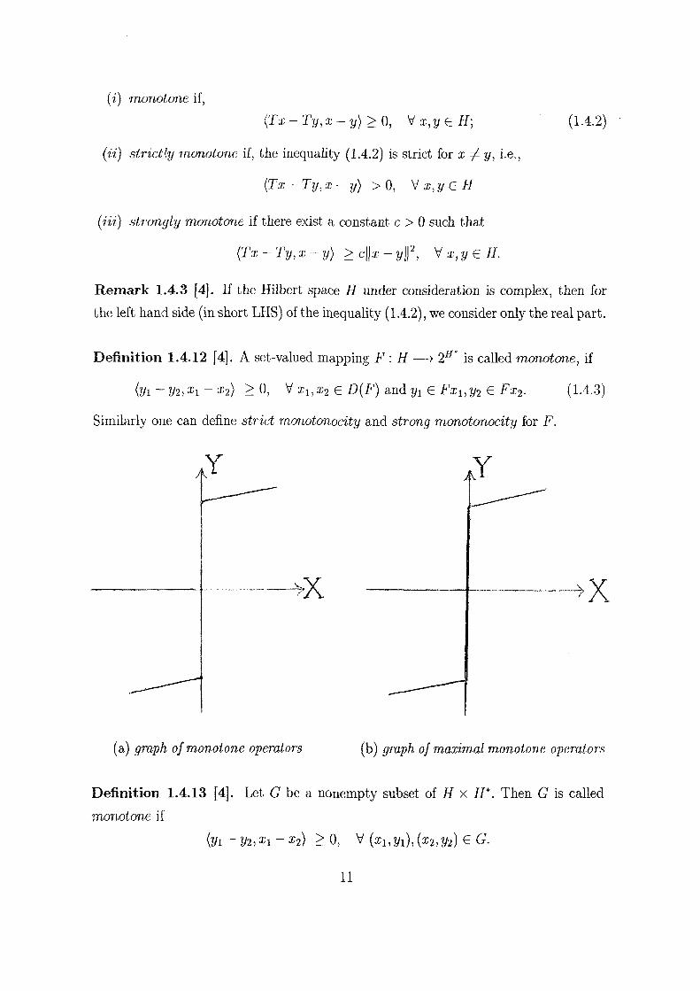
Definition 1.4.12 [4]. A set-valued mapping F : H —> 2^* is called monotone, if

(yi-?/2,3^1-3:2) > 0, Vxi,X2 e Z)(F) and yi e Fxi,y2 e i a;2- (1-4.3)

Similarly one can define strict monotonocity and strong monotonocity for F.

/K Y

^X

A J

^X

(a) graph of monotone operators (b) graph of maximal monotone operators

Definition 1.4.13 [4]. Let G be a nonempty subset of H x H*. Then G is called

monotone if

{yi-y2,xi-X2) > 0 , y ixi,yi),{x2,y2)eG.

11

Definition 1.4.14 [4]. A monotone operator F : H —)• H* is called maximal monotone,

if it has no proper monotone extensions. That is for (x,j/) G -ff x if* we have

{y-v,x-u) >Q, iov all ue D{F),v e Fu.

Then y G Fx.

Similarly, we say that G C H x H* is m,a.xim,al m.onotor),e if for every monotone Gi

such that G C Gi, we have G = G\.

Definition 1.4.15 [35]. A monotone set-valued mapping A is maxim.al if there is no

other set-valued map A whose graph contains strictly the graph of A.

Remark 1.4.4 [35]. A set valued map is monotone (respectively maximal monotone)

if and only if its inverse A"^ is monotone (respectively maximal monotone).

Remark 1.4.5 [35]. By Zorn's lemma, the graph of any monotone set valued map

is contained in the graph of maximal monotone set valued map because the union of

an increasing family of graphs of monotone set valued maps is obviously the graph of

monotone set valued map.

Theorem 1.4.10 [35]. Let H be a reflexive Hilbert space. Let F : H —> 2^* be a

set-valued mapping. Then,

(«') F is monotone (maximal) if and only if G{F) is m,anotone (maximal),

[a) F is monotone (maximal) if and only if F~^ is monotone {maximal).

Theorem 1.4.11 [35]. r et F be a hemicontinuous monotone single valued operator

with D{F) = if, then F is a maximal monotone.

Definition 1.4.16 [35]. A continuous and strictly increasing function 0 : R^ —> R^

is said to be weight function if (plQ) = 0 and Um ^(t) = +oo. t—>-+oo

Definition 1.4.17 [12]. Let (p : R+ —> E+ be a weight function. A set-valued

mapping J : B —)• 2^* is said to be duality mapping of weight </>, if

Jix) = if e B*: (xj) = \\x\\\\fi m^Hwm-12

A selection of the duality mapping J is a single-valued mapping j : B —> B* satisfy­

ing jx G J{x), for each x ^ B. Furthermore, if </>(||a;j|) = |!a:||, Va: e B, then J is called

normalized duality mapping.

Remark 1.4.6 [12]. U B = H, then normalized duahty mapping J becomes identity

mapping.

Theorem 1.4.12 [12]. Let J be a duality mapping associated with a weight function

((), then

(?) J is monotone, that is (x* — y*,x — y) >0, V x, y E B, x* e J(x), y* G J(y)-

(it) J{-x)^-J{x), yxeB.

{Hi) J{Xx) = ~rir^J{x), Vx G 5 and A > 0. (p\\x\\

Definition 1.4.18 [18]. A mapping T : B —> B is said to be

(i) accretive if, y x,y e B, there exists j{x — y) € J{x — y) such thcit

{T{x)~T{y),3{x-y))>Q-

(ii) strongly accretive if, y x,y e B, there exists j{x — y) G J{x — y) such that

{T{x)~T{y)J{x-y))>Q.

(Hi) k-strongly accretive if, V a;, y G B, there exist j{x — y) € J{x — y) and a constant

k > Q such that

{T{x)~T{yli{x~y))>k\\x-y\\\

[iv] 6-Lipschitz continuous if, ^ x,y E B, there exists a constant 6 > 0 such that

\\Tix)-T{y)\\<S\\x-y\\.

Remark 1.4.7. If T is A;-strongly accretive, we have

\\Tix)-T{y)\\>k\\x-y\\.

13

T with the above condition is called k-expanding. Further, if A; = 1, T is called

expanding.

Definition 1.4.19 [18]. A set-valued map F : D{F) CB —> 2^ is said to be

(i) accretive if, y x,y E D(F), u e F{x)^ v e F{y) there exists j{x ^ y) E J{x — y)

such that

{u-v,Jix-y)) >0;

(?'?.) k-strongly accretive if, ^ x,y E D{F), u E F{x),v E F{y) there exists j{x — y)E

J(x — y) such that

{u-v,i{x-y)) > k\\u-vf;

(iii) m-accretive if, F is accretive and (/ + fiF){B) = B for any fixed /i > 0, where /

is the identity mapping on B.

Theorem 1.4.13 [35]. F : H —> 2^ is monotone if and only if (/ + \F) is accretive

for A > 0.

Theorem 1.4.14 [35]. Let F : H —> 2^ is a maximal accretive mapping then

R{F) = H and F"^ is nonexpansive.

We remark that \i F : H —> 2^ is a maximal monotone, then in view of Theorem

(1.4.15) {/ + XF) is maximal accretive for every A > 0 and so we immediately get the

following surjectivity theorems due to Minty [52].

Theorem 1.4.15 [52]. Let F : H —> 2^ be a maximal monotone operator, then

R{I -)- \F) = H and (/ -f AF)~^ is nonexpansive and maximal monotone.

Theorem 1.4.16 [35]. Let F : H —v 2^ be an operator then the following are

equivalent:

(a) F is maximal monotone;

[h] F is monotone and R{I + XF) - H;

14

(c) For every A > 0, (/ + XF) ^ is a nonexpansive mapping defined on whole space

H.

Theorem 1.4.17 [35]. A set-valued mapping F : H —y 2^ is maximal monotone if

and only if the following statements are equivalent:

(a) For every {y,v) G Graph (F), {u — v, x — y) >0]

(6) u e F{x).

Theorem 1.4.18 [35]. Let F : H —> 2^ be maximal monotone mapping then

(a) Its images are closed and convex;

(6) Its graph is strongly-weakly closed in the sense that if Xn converges to x and if

Un e F[xn) converges weakly to u then u E F{x).

Theorem 1.4.19 [35]. Any monotone single valued map T from whole space H to H

which is continuous from H supplied with the strong topology to H supplied with the

weak topology is maximal monotone.

Theorem 1.4.20 [35]. Let F be a monotone set-valued map from H to H. It is

maximal if and only if / -|- F is maximal.

Next we observe that maximal monotone mapping F : H —> 2^ can be approxi­

mated in same sense by single-valued Lipschitzian map Fx from X to X are maximal

monotone, such mapping are called Yosida approximations and plays an important

role.

Theorem 1.4.21 [4]. Let A be maximal monotone. Then for all A > 0, JA = (1 +

AA)"^ is a nonexpansive single valued map from X to X and the map Ax = --(1 — Jx)

satisfies

[i] "^ xeX,Ax{x)eA{Jxx).

(ii) Ax is Lipschitzian with constant with constant - . A

We ako have, for all a; G Dom(A), ||AA(a;) - m{A[x))f < \\m{A{x))f - \\Ax{x)f

and for all x e Dom(A)

15

(i) Jxx converges to x.

(n) A\x converges io m,{A{x)).

Where rn[A{x)) — J l (0) is the element of A{x) of minimal norm.

Definition 1.4.20 [4]. The maps J^ = (1 + XA)'^ and Ax = -{I ~ Jx) are called A

resolvent of A and Yosida approximation of A.

Definition 1.4.21 [76]. A vector space E over the field K{=^ E or C) equipped with

a topology is said to be a topological vector space, if the mappings:

(a) E X E —> £ : [x, y) -)• x + y.

[b] K X E —> E : {a, x) -^ ax.

are continuous, where M (or C) is a set of all real (or complex) numbers.

Definition 1.4.22 [76]. A topological vector space E is said to be Hausdorff if for

every pair Xi,X2 of distinct points of E, there exist neighbourhoods t/j, U2 of Xy and

X2 respectively are disjoint.

Definition 1.4.23 [76]. A topological vector space E is said to be locally convex if

and only if every neighbourhood U oi x £ E is such that, there exists a neighbourhood

V oi E such that V is absolutely convex subset of U.

Definition 1.4.24 (KKM mapping)[76]. Let X be a nonempty subset of a topo­

logical vector space E. A set-valued mapping F : X —^ 2^ is called a KKM mapping n

if Co[xi,X2, ...x^^ C IJ F{xi), for each finite subset {xi,X2,...,a;„}of X,

where CoA denotes the convex hull of set A.

Remark 1.4.8. Observe that if F is a KKM map, then x e F{x).

Theorem 1.4.22 (KKM-Fan Theorem)[76]. Let X be a subset of topological

vector space E. Let F : X -^ 2^ be a set-valued mapping such that F{u) is closed

16

for each u E X, and compact for atleast one u E E. If the convex hull of every finite n

subset {ui,U2, ,Un} of X is contained in the corresponding union (J F(iij), then i = l

n ( ) 0 UGA'

Definition 1.4.25 [76]. A nonempty subset P of a topological vector space £" is said

to be convex cone if,

(a) P + P = P.

(6) AF C P, for all A > 0.

A cone P is to be pointed whenever P n (—P) = {0}.

Definition 1.4.26 [76], A mapping T : H —} H is said to be •j-cocoercive, if there

exists a constant 7 > 0 such that

{T{x)-T{y),x-y) > ^\\Tx~Tyf, V x,y e H.

Theorem 1.4.23 [81]. Let K be a nonempty and convex subset of Hausdorff topo­

logical vector space X and let S : K -^ 2'^ be a set-valued mapping such that

(i) For each u G K S{u) is a nonempty convex subset of K;

(ii) For each v E K, S~^{v) := {uE K : v E S{u)} contains a relatively open subset

O-t, of K, where 0„ may be empty for some v E K;

(iii) U 0, = K-

(iv) K contains a nonempty subset KQ contained in a compact convex subset of Ki

of K such that the set D = \J 01 is compact. (D may be nonempty and 01 veKo

denotes the complement of Ov in K.

Then there exists, UQE K such that UQ E S{UO).

17

Chapter 2

Wiener Hopf Equation and Generalized Mixed Equilibrium Problems

2.1. Introduction

In early nineties, Robinson [73] and Shi [75] initially used Wiener-Hopf equations to

study the variational inequalities. Later on Noor [62-65] used various generahzatioiis

of Wiener-Hopf equations to develop the iterative algorithms for solving various classes

of variational inequahties. An important generalization of Wiener-Hopf equations is

known as resolvent (proximal) equation.

In this chapter, we consider some classes of mixed equiUbrium problems studied

by Moudafi [53] and Kazmi and Khan [42] in real Hilbert spaces. First, we discuss

the some useful generalizations of Yosida approximation. Further using Wiener-Hopf

equation technique we discuss the sensitivity analysis relying on a fixed point formu­

lation of the given problem. Such formulations are obtained using generalizations of

the Yosida approximation which allow us to derive some iterative methods for these

problems. This chapter is based on work of Moudafi [53] and Kazmi and Khan [42].

The remaining part of this chapter is organized as follows.

In Section 2.2, we consider a mixed equihbrium problem so called general mixed

equiUbrium problem [53] in Hilbert space. We discuss some properties of a general­

ization of Yosida approximation. Further using Wiener Hopf equation technique we

discuss the sensitivity analysis relying on a fixed point formulation of the given prob­

lem. In Section 2.3, we develop an iterative algorithm for the general mixed equiUb­

rium problem and discuss its convergence analysis. In Section 2.4, we consider a mixed

equilibrium problem [42] involving set-valued mappings called generaUzed mixed equi­

librium problem in Hilbert space. We discuss some properties of a generalization of

Yosida approximation. Further using Wiener Hopf equation technique we construct an

iterative algorithm for the generaUzed mixed equilibrium problem relying on a fixed

18

point formulation of the given problem. In Section 2.5, we give the existence of solu­

tion of generalized mixed equihbrium problem and discuss the convergence and stability

analysis of the iterative algorithm.

2.2. Sensitivity Analysis of General Mixed Equilibrium Problem

Throughout the chapter unless otherwise stated, let H he a. real Hilbert space with

its topological dual H*; let 2^ be the power set of H; CB{H) denotes the family of

all non emjity closed and bounded subsets of H. If there is no confusion, we denote

the norm of Hilbert space H and its dual space H* by ||.||, and the inner product of H

and the duality pairing between H and H* by {.,.).

Let K be a nonempty convex and closed subset of H. Given that T,g : K —> K

are nonhnear mappings and F : K x K —5- R is a bifunction satisfying F{x,x) =

0, V X e K. Consider the general mixed equilibrium problem (in short, GMEP) of

finding x G K such that

F{g{x),y) + {Tx,y~gix))>0, V y E K. (2.2.1)

Now we give following concepts and results which are needed in the sequel.

Definitioii 2.2.1. Let F : K x K —> Rhe a real valued bifunction.

(?) F is said to be monotone, if

F{x,y) + F{y,x)<0, \/x,y e K;

{a) F is said to be strictly monotone, if

F[x,y) + F{y,x) < 0, ^ x,ye K with a; / y;

[Hi) F is upper hemicontinuous if for aU. x,y,z E K,

lim sup F{tz + {1 - t)x,y) < F{x,y).

Theorem 2.2.1. If the following conditions holds true:

19

(i) F is monotone and upper hemicontinuous;

(n) F{x,.) is convex and lower hemicontinuous for each x e K;

[in) There exists a compact subset B of H and there exists yo E B f) K such that

F{x,yo) < 0 for each x e K\B.

Then the set of solutions of the following problem:

Find xeK such that F{x, y) > 0 ^ y e K, (EP)

is nonempty convex and compact.

Remark 2.2.1. If F is strictly monotone, then the solution of (EP) is unique.

Now we define a generalization of Yosida approximation and discuss its properties.

Definition 2.2.2. Let // be a positive number. For a given bifunction F the associated

Yosida approximation, F^ over K and the corresponding regularized operator A^, are

defined as foUows:

^^"M( 'y) = (-{^- Jjl{^)),y -x) and Af^{x) = -{x- ./^(a;),

in which -/,f (••y) E K is a unique solution of

l^F[Jl{x),y) + {J^[x) -x,y- JJ^ix)) > 0, VyeK (2.2.2)

Remark 2.2.2.

(i) The existence and uniqueness of the solution of problem (2.2.2) follows by invok­

ing Theorem 2.1.1 and Remark 2.1.1.

[ii) Observe that in the case where F{x,y) = sup {C,,y — x) and K = H, B being a CeSx

maximal monotone operator, it directly yields

jP{x) = (/ + ^jiB)~'x and Aj(x) = B^{x),

where Bn = -{I -{I + /i-B)~^) is the Yosida approximation of B and we recover

the classical concepts given in Definition 1.4.20.

20

Defintion 2.2.3. A mapping M is c-firmly nonexpansive (c being a positive constant)

if for all x,y G H

\\M{x) - M(y) f < \\x - y\\ - c||(/ - M)x -(I- M)yf.

Theorem 2.2.2. Assume that the conditions of Theorem 2.2.1 are fulfilled, then the

operator J j is cocoercive with modulus 1, that is,

{j;{^) - 4{y),^ -y)> \\J'{^) - J'ivW, V ,y e H; (2.2.3)

J^ is l-firrnly nonexpansive, namely:

!l<(^) - J'ivW < Ik - yf - \\{i -J',)^ -{I- J^yf (2-2-4)

and A^ is cocoercive with modulus fi, namely:

« ( ^ ) - <(2/ ) ,^ - y) > /^llAj(x) - A'^{y)f, yx,yeH (2.2.5)

Now, in the relation to general mixed equihbrium problem (GMEP), we consider

the following Wiener-Hopf equation (in short, WHE):

Find zeH such that T(x) + A^{z) = 0 and g{x) = J^z. (2.2.6)

The following theorem shows that GMEP (2.2.1) is equivalent to WHE (2.2.6).

Theorem 2.2.3. The GMEP (2.2.1) has a solution a: 6 i^ if and only if WHE(2.2.6)

has a solution z £ H, where

g{x) = J^z and z ^ g{x) - nT{x}. (2.2.7).

Further we have following fixed point formulation of GMEP (2.2.1).

Theorem 2.2.4. x e K solves (MEP) if and only if x satisfy the relation

g{x) = J^{g{x) - fxT{x)).

In the sequel, we assume that the the bifunction F satisfies condition of Theorem

2.2.1.

21

Next we discuss the sensitivity analysis of solution of GMEP (2.2.1).

In recent years, much attention has been given to develop general techniques for

the sensitivity analysis of solution set of various classes of variational inequalities (in­

clusions). From the mathematical and engineering point of view, sensitivity properties

of various classes of variational inequalities can be provide new insight concerning the

problem being studied and can stimulate ideas for solving problems. The sensitivity

analysis of solution set for variational inequalities have been studied extensively by

many authors using quite different techniques. By using the projection technique, De-

fermos [17] studied the sensitivity analysis of solutions of variational inequalities with

single-valued mappings. By using the implicit function approach that makes use of so-

called normal mappings (Wiener-Hopf equation), Robinson [73] studied the sensitivity

analysis of solutions for variational inequalities in finite-dimensional spaces. By using

projection and proximal-point mappings techniques, Ding and Luo [22|, Liu et al. [51],

Park and Jeong [72], Ding [21], and Kazmi and Khan [43], studied the behavior and

sensitivity analysis of solution set for some classes of generahzed variational inequahties

(inclusions).

Now, we consider the parametric versions of GMEP (2.2.1) and WHE (2.2.6). To

formulate t,here problems, let A be an open subset of H in which A takes values then

the parametric version of GMEP (2.2.1) is given by

MdxxeH suchthat F(p(xA,A),y,A) + (T(:rA,A),|/-x) > 0 , (2.2.8)

where T(.,.) : F x A-^ K, and F(.,. , .) : (K x if) x A -^ M are given mappings.

The associated Wiener-Hopf equation is

find z, e H : T{x,,X) + (Aj(., A))^ZA = 0 and g{x,, A) = j;^^-'h,. (2.2.9)

We suppose that for some A G A problem (2.2.8) has a unique solution x which is

equii'alent, by Theorem 2.2.3 to assuming that equation (2.2.9) has a unique solution

z. In what follows we are intrested in knowing if equation (2.2.8) (respectively (2.2.9))

has a solution denoted Xx (respectively, zx,) close to x (respectively, z) when A is close

to A, and how the function x(\) = a:^(respectively, z{X) = zx) behaves. In other words

we want to investigate the sensitivity of the solution a;, z with respect to the change of

parameter A.

22

Now let r be a closed convex neighbourhood of z. We will use the alternative fixed

point formulation given in Theorem 2.2.4 to study the sensitivity of problems (2.2.8)

and (2.2.9). More precisely, we want to investigate those condition under which, for

each z\ near z (respectively, x\ near x) the function z\ = z(A) (respectively, x\ — a (A))

is continuous or Lipschitz continuous.

Definition 2.2.4. Let T be a operator defined on F x A. Then for all x^y EV^ the

operator is said to be

{%) locally a-strongly monotone if there exists a constant ct > 0 such that

( r ( x , A ) - T ( t / , A ) , x - | / ) > a | | x - t / f ;

i(ii) locally (3-Lipschitz continuous if there exists a constant ^ > 0 such that

\\T{x,X)-T{y,X)\\<(3\\x-y\\.

It is clear that a < p.

We consider the case, when the solution of the parametric Wiener Hopf equation

(2.2.9) lie in the interior of F. Following the ideas of Dafermos [17], we consider the

map

G{z,X) = 4^'^-''\z,)-fiT{{x,,X))

^g{x,,X)-^T{{xx,X)). (2.2.10)

Where g{xx,X) = J?^ ' '^^(ZA) and Fp : {K nT) x {K nV) x A -^ K with F|r = F.

We have to show that the map z -4- G{z,X) has a fixed point, which is also a

solution of (2.2.9). First of all, we prove that the map is a contraction with re­

spect to z uniformly in A E A by using assumption (i) and (ii) on the operators

r ( . , A) and g{., A) defined on F x A

Theorem 2.2.5, Let the operator r ( . . A) be a locally a-strongly monotone locally

/^-Lipschitz continuous and g{.,X) he locally ^-strongly monotone locally <7-Lipschitz

continuous with constant, if

1 - A; > 0, a> 2f3y/k{l - k), and | /i - -^ l< a ./^^-Ak{l-k)(3^

^ 2 I ^ ^ 2

23

then for all 7.\,zi e F and A e A, we have

| |G'(zi ,A)-G(z2,A)| |<ei |2i-^2| | (2.2.11)

where

k := V l - 2 5 + a2 and ^ = ^ + ^"^ " ^ ^ + ^'^'- (2.2.12)

Remark 2.2.3. Since z is a solution of (2.2.9) for A = A, it is then easy to show that

z is the unique fixed point in F of the map G(., A). In other words

z = z{\ = G[z{\),\) (2.2.13)

Using Theorem 2.2.5 we prove the continuity of the solution z(A) (respectively, a;(A))

of (2.2.9) (respectively (2.2.8)) which is main motivation of the next result.

Theorem 2.2.6. If the operators T{x^.) and 5(., A) are continuous (or Lipschitz con­

tinuous), then the function z{X) is continuous (or Lipschitz continuous) at A = A. If in

addition the map A -^ J ' ' z is continuous (or Lipschitz continuous), the function

x{X) is in turn continuous (or Lipschitz continuous) at A = A.

Theorem 2.2.7. If the assumption of Theorem 2.2.5 holds true, then there exists a

neighborhood iV C A of A such that for all A G iV, z(A) (respectively .x(A)) is a unique

solution of (2.2.9) (respectively (2.2.8)) in the interior of F.

Theorem 2.2.8. Let x be a solution of the parametric mixed equilibrium problem

(2.2.8) and z the solution of the parametric Wiener-Hopf equation (2.2.9) for A = A.

Let r ( . . A) and </(., A) be a locally strongly monotone and locally Lipschitz continuous

operator on F. If the operator T{x^ X),g(x, A) are continuous (or Lipschitz continuous)

at A = A, then there exists a neighborhood iV c A of A such that for A E AT, (2.2.9)

has a unique solution z{X) in the interior of F, z(X) = z and z(A) is continuous (or

Lipschitz continuous) at A = A.

If in addition the map A -> JfJ^ ' z is continuous (or Lipschitz continuous) at

A = A, then for X E N, the parametric problem (2.2.8) has s unique solution a:(A) in

the interior of F, x{X) = x and (A) is continuous (or Lipschitz continuous) at A = A.

24

2.3. Iterative Algorithm and Convergence Analysis

In this section, we use fixed point formulation of GMEP(2.2.1) given by Theo­

rem 2.2.5 to develop an iterative algorithm for finding the approximate solution of

GMEP(2.2.1). Further we discuss the convergence analysis of the iterative algorithm.

More precisely, we apply approximation method to solving x = p(a;), where

p{x) = x-g{x) + J;;{g{x)-^iT{x)).

The resulting procedure follows.

Iterative Algorithm 2.3.1. Given XQ G K, compute the point Xk+i by

^k+i =Xk- g{xk) + J^{g{x) - pT{x)). (2.3.1)

where /i. > 0 is a constant.

Theorem 2.3.1. Let the operator T be a-strongly monotone /?-Lipschitz continuous

and g be <5-strongly monotone, o"-Lipschitz continuous. If the parameters satisfy con­

dition (2.2.11), then Xk+i is well defined and the sequence {x^} strongly converges to

a solution of GMEP(2.2.1).

Theorem 2.3.2. Let T be a cocoercive operator with constant 7. If ^ < 27, then the

sequence {xfe} weakly converges to a solution of GMEP(2.2.1).

Remark 2.3.1.

(i) Observe that when the operator is a gradient, then cocoercivity property is equiv­

alent to a simple monotonicity plus Lipschitz continuity. But this equivalence is

not true in general, indeed the rotation by — is not cocoercive although it is

monotone and Lipschitz.

[ii) It is easy to check that when an operator is strongly monotone and Lipschitz,

then it is cocoercive. So we may say that for Lipschitz operators, the cocoercivity

is a weaker than the strong monotonicity.

25

2.4. Generalized Mixed Equilibrium Problems

In this Section, we consider a generalized mixed equilibrium problem [53] involving

set-valued mappings in Hilbert space. We discuss some properties of a generalization

of Yosida approximation. Further using Wiener liopf equation technique we construct

an iterative algorithm for the generalized mixed equihbrium problem relying on a fixed

point formulation of the given problem. In Section 2.5, we prove the existence of

solution of generalized mixed equihbrium problem and discuss the convergence and

stabihty analysis of the iterative algorithm.

Let F : KxK ^Rhe a bifunction such that F(x, x) = 0, Va; e K; let g : K -^ K

and r},N : H Ys H -^ H he nonlinear mappings and hi T,B : H -^ CB{H) be

set-valued mappings, then we consider the following generahzed mixed equihbrium

problem involving non-monotone set-valued mappings with non-compact values (in

short, GMEP):

Find X G K, u eT(x), v G A{x) such that

F{g{x),y) + {N{u,v),r]{y,g{x))) > 0, Vy e K. (2.4.1)

Some Special Cases:

1. If F{x,y) = 4'{y,x) " 0(a^,a;), Vx,|/ € K, where (j) : K -^ M. is a. real-valued

function, then GMEP (2.4.1) reduces to the generahzed variational inequahty

problem of finding x E K, uE T{x), v 6 B{x) such that

{N{u,v),'r){y,g{x))) + ^{y,x) - <P{g{x),x) > 0, Vt/ 6 K.

Similar problem has been studied by Ding [23].

2. If T,B are single-valued; N{T{x),B{x)) = C{x), where C : H -^ H, and

r]{y,x) = y — X, yx,y E H, then GMEP (2.4.1) reduces to the general mixed

equihbrium problem (2.2.1).

Now, we give an extension of the Yosida approximation notion introduced in [53,55].

Definition 2.4.1. Let p > 0 be a number. For a given bifunction F, the associated

Yosida approximation, Fp, over K and the corresponding regularized operator, A^, are

defined as follows:

F,{x,y) = ( i ( x - J^ix))My,^)) and A^{x) = -^{x - J^{x)), (2.4.2)

in which J.f (a;) e K is the unique solution of

pF{J^{x),y) + {j;;\x) - x,ii{y, jj^ix))) > 0, V?/ e K. (2.4.3)

Remark 2.4.1. If F satisfies all conditions of Theorem 2.2.1 and Remark 2.2.1, then

problem (2.4.3) has the unique solution.

Remark 2.4.2.

(i) \i K = H and F{x,y) = sup (C,''?(y,3;)), Va;,y e K, where M is maximal

strongly 7y-monotone operator, then it directly yields

J^{x) = {I + pMy\x) and AJ(X) = Mp{x),

where Mp := - (I — (I + pM)"^) is the Yosida approximation of M. In this

case Jp generalizes the concept of resolvent mapping for single-valued maximal

strongly monotone mapping given in Li and Feng [48].

(ii) If //(y, x) = y — X, Va;, y E H, then Definition 2.4.1 reduces to Definition 2.2.2.

Theorem 2.4.1. Let the bifunction F : K x K -^ Rhe a-strongly monotone and

satisfy the conditions of Theorem 2.2.1, and let the mapping rj : H x H -^ H he

(5-strongly monotone and r-Lipschitz continuous with r]{x,y) +r]{y,x] = 0, Va;,y € H,

then the mapping J j is ^-^-Lipschitz continuous and Af^ is c-cocoercive for c =

— { i + ( ? ^ ) . 2 } '

Now, related to GMEP (2.4.1), we consider the following generalized Wiener-Hopf

equation problem (GWHEP):

Find 2 6 //, a; e A', ti 6 T{x), v E B{x) such that

Niu,v) + A;:{Z) = 0 and g{x) = J^iz). (2.4.4)

Theorem 2.4.2. GMEP (2.2.1) has a solution {x,u,v) with x e K, u e T{x), v e

B{x) if and only if (a;, M, V) satisfies the relation

g[x) = Jl[g{x)-iiN{u,v)\.

27

Theorem 2.4.3. GMEP (2.4.1) has a solution {x,u,v) with x e K, u E T{x), v e

B{x) if and only if GWHEP (2.4.4) has a solution {z,x,u,v) with z e H, where

g{x) = j ; ( z ) (2.4.5)

and

z = g{x) ~ fj,N{u,v). (2.4.6)

The GWHEP (2.4.2) can be written as

which implies that

z = J^{z)~^N{u,v),

= g{x)-^N{u,v), by (2.4.7).

This fixed point formulation allows us to construct the following iterative algorithm.

Iterative Algorithm 2.4.1. For a given ZQ G H, we take XQ E K such that

Let UQ e r(a;o), VQ G B(XO), and Zi = (1 — A)2o + ' [ '( ^o) ~ ^ -^(^ ,^0)] , where

0 < A < 1 is a relaxation parameter.

For ^1, we take Xi E K such that g{;Xi) = Ja{zi)- Then by Theorem 2.1, there exist

Ml e T{xi), Vi e B{xi) such that

Wui-M] < {l + l)n{Tix,),T{xo)),

I h - ^ o l l < {l + l)'H{B{x,),B{xo)).

Let

22 = ( l - A ) z i + Aig(xi)-|xiV(«i,t;i)].

By induction, we can obtain sequences {z„}, {a n}) {w„} and {i/„} defined as

5(x„) = J^izr^l (2.4.7)

x n e r ( x „ ) : | K + x - « n | | < (l + ( l + n ) - ^ ) niT{xn+i),TM), (2.4.8) ttr,

28

VneB{Xn): Ik+l-^^nli < (l + (1 + Tl)" ) n{B(Xn+l), B{Xr,)), (2.4.9)

Zn+l = (1 - X)Zn - X[g{Xn) - / /A^K, f n)] , (2.4.10)

where n = 0,1,2,..; / > 0 is a constant and 0 < A < 1 is a relaxation parameter.

2.5. Existence of Solution, Convergence Analysis and Stability

We prove the existence of solution of GWHEP (2.4.4) and discuss the convergence

analysis and stability of Iterative Algorithm 2.4.1.

Definition 2.5.1. Let G : ^ 2^ be a set-valued mapping and XQ € E. Assume

that a;„+i G f{G, x„) defines an iteration procedure which yields a sequence of points

{xn} in E. Suppose that F{G) = {x G E : x E G{x)} 7 0 and {xn} converges to some

X G G(x). L<3t {?/„} be an arbitrary sequence in E, and e„ = (|?/n+i ~ n+ijj, ^n+i G

/{G, Xn).

(i) If Um €„ = 0 implies that lim yn — x, then the iteration procedure Xn-^-i G n—>-oo n—j-oo

f(G,Xn) is said to be G-stable.

0 0

(ii) If €n < 00 implies that lim y^ = x, then the iteration procedure Xn+i G n=0 '''-^°°

f{G,Xn) is said to be almost G-stable.

Remark 2.5.1.

(i) Definition 2.5.1 can be viewed as an extension of concept of stability of iteration

procedure given by Harder and Hicks [33].

(ii) Recently, some stabihty results of iteration procedures for variational inequahties

(inclusions) have been established by various authors.

The following Theorem is used to prove the main result of this section.

Theorem 2.5.1 [50]. Let {a„}, {&„} and {cn} be nonnegative real sequences satisfying

a„+i = (1 - Xn)an + XnK + Cn, Vu > 0,

where CX3 oo

E A„ = oo; {Xn} C [0,1]; lim 6„ = 0 and } c„ < oo. x=0

29

Then lim an = 0. n-+oo

Theorem 2.5.2. Let iv be a nonempty, closed and convex subset of H] let the

mapping t] : H x H ^ H he (^-strongly monotone and r-Lipschitz continuous with

r]{x,y) + f?(;t/,a;) = 0, Vx,y E H; let the bifunction F : K x K -^ R he a-strongly

monotone and satisfy the assumptions of Theorem 2.2.1; let the mapping A : H x H -^

H be ((7i,cr2)-Lipschitz continuous; let the mappings T,B : H ^ CB{H) he Hi-H-

Lipschitz continuous and /J2-'H-Lipschitz continuous, respectively, and the mapping

g : K -^ K he 7-strongly monotone and ,^-Lipschitz continuous. If the following

conditions hold for fi > 0: b(S - r) , ,

/i < ^ f; 2.5.1 er — ab

er <ah] b> 0. (2.5.2)

where e := (Ji/ii + (T2/X2 and 5 = 1 — y/l — 27 + ^'^.

Then the sequences {zn}, {xn}, {un}, {vn} generated by Iterative algorithm 2.4.1

strongly converge to z ^ H, x E H, u e T{x), v e B[x), respectively, and (z, .x, M, •?;)

is a solution of GWHEP (2.4.4).

Theorem 2.5.3(stability). Let the mappings 7;, F\ N,T, B,g be same as in Theorem

2.5.1 and conditions (2.5.1), (2.5.2) of Theorem 2.5.1 hold with e = {l+e){aifii+a2ft2).

Let {QU} be any sequence in / / and define {a„} C [0,00) by

giVn) = M (9")'

£n e T[yn) : ||«n+i - u^W < (! + (! + n)-') 7{(r(y„+i),T(y„))

neBivn) : \\vn+i-Vn\\ < (l + (1 + n)"!) H(B(2/„+i),B(y„,)))

= I k n + l - (1 - A)g„ - X[g{yn) - nN{Un,Vn)\\\,

u.

V

a.

where n = 0,1,2,....; // > 0 is a constant and 0 < A < 1 is a relaxation parameter.

Then lim (g„, ?/«, w„, w„) = [z, x, u, v) if and only if lim a„ = 0, where (z, x, u, v) is a n—>oo n—i-oo

solution of GWHEP (2.4.4).

30

Chapter 3

Resolvent Dynamical Systems for Mixed Equilibrium Problems

3.1. Introduction

In recent past, much attention has been given to consider and analyze the projected

dynamical system associated with variational inequalities and nonlinear programming

problem, in which the right hand side of the differential equation is a projection op­

erator. Such type of the projected dynamical system were introduced and studied by

Dupuis and Nagurney [25]. Projected dynamical systems are characterized by discon­

tinuous right-hand side. The discontinuity arises from the constraints governing the

question. The innovative and novel feature of a projected dynamical system is that its

variational inequality problems. It has been shown in [57,82,83] that the dynamical sys­

tem are useful in developing efficient and powerful numerical technique for solving the

variational inequahties and related optimization problems. Xia and Wang [83], Zang

and Nagureny [85] and Nagureny and Zang [58] have studied the globally asymptotic

stability of these projected dynamical systems. Noor [61-63] has also suggested and

analyzed similar resolvent dynamical system for variational inequalities. Very recently,

Kazmi and Khan [43] studied dynamical system for mixed equilibrium problem. In

this chapter, we discuss dynamical systems for the mixed equilibrium problems. This

chapter is based on the work of Kazmi and Khan [43].

The remaining part of the chapter is organized as follows:

In Section 3.2, we consider a mixed equilibrium problem (MEP) in M" and give its

related Wiener-Hopf equation (WHE) and fixed-point formulation. Further, using this

fixed-point formulation and WHE, we consider a resolvent dynamical system associated

to MEP (in short, RDS-MEP). Furthermore, we review some concepts and result which

are needed in the sequel. In Section 3.3, using Gronwall inequality, we discuss existence

theorem for RDS-MEP. Further, we discuss that RDS-MEP is solvable in sense of

Lyapunov and globally converges to the solution set of MEP. Furthermore, we discuss

that RDS-MEP converges globally exponentially to the unique solution of MEP.

31

3.2. Mixed Equilibrium Problems and Dynamical Systems

Let K" be a Euclidean space, whose inner product and norm are denoted by (.,.)

and j | . jl respectively. Let K he a nonempty, closed and convex set in M"; T, A : /f -> iv

be nonlinear mappings, and N : KxK -^ K be a nonlinear mapping, li f : KxK -^M.

is a given bifunction satisfying f{x,x) — 0 for all x E K. Consider the ibllowing mixed

equilibrium problem (MEP): Find x e K such that

f{x,y) + {N{Tx,Ax),y-x)>0, ^y E K. (3.2.1)

Some Special Cases:

1. If N{Tx,Ax) = Sx, Vx e K, where S : K ^ K, then MEP (3.2.1) reduces to

the mixed equihbrium problem (1.3.1).

2. If F{x,y) = sup (w,y — x) with B : K —> 2^' a set-valued maximal monotone

operator. Then MEP (3.2.1) is equivalent to find x G K such that

QEN[TX,AX) + BX, yyeK,

which is known as variational inclusions.

Theorem 3.2.1. MEP (3.2.1) has a solution x if and only if x satisfies the equation

X = J^(x- - p,N{Tx, Ax)), for /i > 0.

We now define the residue vector R{x) by the relation

R{x) =x~ Jl[x - iiN{Tx, Ax)]. (3.2.2)

Invoking Theorem 3.2.1, one can observe that x G i^ is a solution of MEP (3.2.1)

if and only if x E K is a zero of the equation

R{x) = 0. (3.2.3)

Now related to MEP (3.2.1), we consider the following Wiener-Hopf equation

(WHE): Find z^W such that for x e K,

N{Tx,Ax) + Al{z)^0 (3.2.4)

32

and

x = Jl{z), for ^L>Q. (3.2.5)

Theorem 3.2.2. MEP (3.2.1) has a solution x if and only if WHE (3.2.3)-(3.2.4) has

a solution z € M' where

X = Jliz) (3.2.6)

and

2 = a; - lxN{Tx, Ax), for /i > 0. (3.2.7)

Using (3.2.5)-(3.2.6), WHE (3.2.3)-(3.2.4) can be written as

N{Tx, Ax) -Jl[x- fiN{Tx, Ax)]

+piN{T{Jl[x - ixN{Tx, Ax)\), ^(j/[x- - piN{Tx, Ax)])) = 0. (3.2.8)

Thus it is clear from Theorem 3.2.2, that x e K \s a solution of MEP (3.2.1) if

and only li x E K satisfies the equation (3.2.7).

Using this equivalence, we suggest a new dynamical system associated with MEP

(3.2.1) is defined as

dx

It - = X{Jl\x~fiN{Tx,Ax)

-fj,N(T{J^[x - nN{Tx, Ax)]), A{Jl[x - ^N[Tx, Ax)])) + iJiN{Tx, Ax) - x),

= X{-R[x) + iiN{Tx, Ax)

-li,N{T{Jl\x - fiNiTx, Ax)]), A{Jl[x - f^N{Tx, Ax)]))}, xih) ^ XQ e K,

(3.2.9)

where A is a constant. The system of tj^e (3.2.9) is called the resolvent dynamical

system associated with mixed equilibrium problem (3.2.9), (for short, RDS-MEP).

Here the right-hand side is associated with resolvent and hence in discontinuous on the

boundary of K. It is clear from the definitions that the solution to (3.2.9) belongs to

the constraints set K. This implies that the results such as the existence, uniqueness

and continuous dependence on the given data can be studied.

33

3.3. Existence and Stability of a Unique Solution of Dynamical System

First we give the following concepts and results which are useful in the sequel.

Definition 3.3.1. The dynamical system is said to converge to the solution set K*

of MEP (3.2.1) if and onl}^ if, irrespective if the initial point, the trajectory of the

dynamical system satisfies

limdist(x(i),A'*),

t-4oo

where

dist{x,K*) = inf \\x-y\\. y&K*

It is easy to see that, if the set K* has a unique point x*, then (3.2.9) implies that

lim xii) = X*. t->oo

If the dynamical system is still stable at x* in the Lyapunov sense, then the dy­

namical system is globally asymptotically stable at x*.

Definition 3.3.2. The dynamical system is said to be globally exponentially stable

with degree: T] at x* if and only if, irrespective of the initial point, the trajectory of t,lie

system x{t) satisfies

\x (t) - x*\\ < fi4x{to) - x*\\ expi~r]{t - to)), V > ^o,

where Hi and rj are positive constants independent of the initial point. It is clear that

globally exponentially stabihty is necessarily globally asymptotical stability and the

dynamical system converges arbitrarily fast.

Theorem 3.3.1 [32]. Let x and y be real-valued nonnegative continuous function

with domain {t: t < to} and let a[t) — aodt — io|), where ao is a monotone increasing

function. If, for t>to,

X < a{t) + I x{s)y{s)ds, Jto

then ^

x{s) < a{t) + exp ({ / y{s)ds}).

34

Definition 3.3.3. Let T,A : K -^ K, f : K x K -> R, a.nd N : K x K -> K he

nonlinear mappings. Then, for sll x,y,z,w G K,

(a) T is S-Lipschitz continuous if there exists a constant 8 > Q such that

| | T x - T y | | < l | a : - y | ! ;

(b) A' is {a,l3)-Lipschitz continuous if there exist constants ct,/? > 0 such that

\\N{x,y) - N{z,w)\\ < a\\x - z\\ + (3\\y - w\\-

(c) A is mixed monotone with respect to T and A, if

{N{Tx,Ax)-N{Ty,Ay),x-y)>0;

(d) / is said to be 9-pseudomonotone, where ^ is a real-valued multivariate function,

if

/ ( a ; , y ) + ^ > 0 implies ~f{y,x) + 9>0.

In the sequel, we assume that the bifunction / involved in MEP (3.2.1) satisfies

conditions of Theorem 2.2.1. Further, from now onward we assume that K* is nonempty

and is bounded, unless otherwise specified. Furthermore, assume that for ail x E K,

there exists a constant r > 0 such that

||Ar(ra;,Aa;)|| < T(||Trr|| + p x | | ) .

We study the some properties of RDS-MEP (3.2.9) and analyze the global stabihty

of the system. First of all, we discuss the existence and uniqueness of RDS-MEP (3.2.9).

Theorem 3.3.2. Let the mappings T, A and A be (^-Lipschitz continuous, 7-Lipschitz

continuous and {a, /3)-Lipschitz continuous, respectively. For each a:o ^ IR", there exists

a unique continuous solution x{t) of RDS-MEP (3.2.9) with x(tQ) = t^ over [to, 00).

We now study the stabihty of RDS-MEP (3.2.9). The analysis is in the spirit of

Xia and Wang {83].

Theorem 3.3.3. Let the mappings T, A and N be the same as Theorem 3.3.2. Let

the function / be ^-pseudomonotone with respect to 9, where 9 is defined as

9{x,y) = {N{Tx,Ax),y^x), ^x,yeK,

35

and let A be mixed monotone with respect to T and A. If /i < ^^!«. x, then RDS-MEP

(3.2.8) is stable in the sense of Lyapunov and globally converges to the solution set of

MEP (3.2.1).

Theorem 3.3.4. Let the mappings T,A and N be the same as Theorem 3.3.2. If

A < 0, then RDS-MEP (3.2.9) converges globally exponentially to the unique solution

of MEP (3.2.1).

36

Chapter 4

Auxiliary Principle Techniques for Mixed Equilibrium Problems

4.1. Introduction

One of the most important and interesting problem in the theory of mixed equi­

librium problems is to develop the methods which give efficient and implementable

algorithms ibr solving mixed equilibrium problems. These methods include projection

method and its variant forms, hnear approximation, descent, and NcM ton's methods,

and the method based on auxiliary principle technique.

It is well known that the projection method and its variants can not be extended

for mixed equilibrium problems involving non-differentiable term. To overcome this

drawback, one uses usually the auxiliary principle technique. This technique deals

with finding a suitable auxihary principle and prove that the solution of an auxiliary

problem is the solution of the original problem by using the fixed-point approach.

Glowinski, Lions and Tremolieres [31] used this technique to study the existence of a

solution of mixed variational inequalities. Cohen [13], Zhu and Marcotte [86], Noor

[61-67], Huang and Deng [34], Chidume et al. [11] extended this technique to suggest

and analyze a number of iterative methods for solving various classes of mixed equilib­

rium problems. In this chapter, we discuss auxiliary principle techniques and viscosity

method for some mixed equilibrium problems. This chapter is based on the work of

Moudafi and thera [55], Moudafi [54] and Kazmi and Khan [44].

The remaining part of this chapter is organized as follows.

In Section 4.2, we consider a mixed equilibrium problem (MEP) in Hilbert space

and discuss the convergence analysis of the proposed iterative method based on an algo­

rithmic approach. In Section 4.3, we discuss viscosity method in order to approximate

a solution of mixed equilibrium problem (MEP). In Section 4.4, we studies general­

ized mixed equihbrium problem (GMEP) involving non-differentiable term in Hilbert

space and discuss some of its special cases. Further, we discuss an auxihary problem

related to GMEP and give some concepts. Furthermore, we discuss an existence and

37

uniqueness theorem for the auxihary problem. In section 4.5, we have an algorithm

for GMEP and we discuss the convergence analysis of the algorithm and existence of

solution of GMEP.

4.2. Auxiliary Problem for Mixed Equilibrium Problem

Let K be a nonempty convex closed subset of a real Hilbert space H, F : KxK —>

JK is a given bivariate function with F(x, x) = 0, for all x e K and T : K —> IR is a

continuous mapping. We consider the following mixed equilibrium problem (MEP)[53]:

Find X E K such that

F{x,x) + {T{x),x-x)>{), \/xeK. (4.2.1)

Let A be a given number and consider a given iterates x^. The auxiliary problem for

mixed equilibrium problem consists of determining Xk+i £ K which satisfies:

F{xk+ux) + {T{xk) + X-\h'{xk+i) - h'{xk)),x - Xfc) > 0 V a; e K, (4.2.2)

where h' is the derivative of a given strictly convex function on K. We use a cocoer-

civity condition on T to analyze the convergence beha\aor of the proposed iterative

method based on an algorithmic approach induced by Cohen as "the axillary problem

principle" for optimization and variational inequalities.

Definition 4.2.1. A space X is said to satisfy the OpiaVs condition, if for each

sequence {xn}'^=i in X which converges weakly to a point x e X,we have

hm inf l|a;„ - x|| < lim inf llx„ -y\\, Vy e X, y / x.

Theorem 4.2.1. Let F be a upper hemicontinuous monotone bivariate function over a

closed convex set K such that F{x,.) is convex and lower semi continuous for all x e K.

let h be a-strongly convex over K and its derivative /i', be /3-Lipschitz continuous. We

suppose that T is 7-cocoercive over K, i.e.,

{T{x)-T{y),x-y)> ^\\T{x)-T{y)\\\ ^ x,y e K

38

then there exists a unique solution Xk+i to the auxiliary equihbrium problem (AEP).

Furthermore, if 0 < A < 2aj, then the sequence {xk}keN weakly convei~ges to a solu­

tion of the considered problem.

Remark 4.2.1.

[i) The previous convergence theorem is an extention of a result by Zhu and Marcotte

[86] and it is worth mentioning that if T is a single-valued mapping, by taking

F{x, y) = (^x,y — x), we recover as a special case the auxiliary problem principle

of G.Cohen [13].

[ii) It should be noticed that inexact version are essential for producing imple-

mentable methods since, except for very special situations, the auxiliary equi­

hbrium problem may be solved exactly. So it is essential to replace the iterative

scheme (AEP) by a relation which takes into account an approximate calculation

of the iterates. More precisely, one can consider the following method: At stage

k, starting from x^., compute a solution of

{Fxk+i,x) + {T{xk) + \-\li!{xk+i) - [h'{xk)),x- Xk+i) >-€k y xeK

where {ek}keN is a sequence of positive numbers which goes to zero. The conver-+00

gence result above still holds true provided that X] f/t < +oo.

Theorem 4.2.2. In addition to hypothesis on F, K and /i, we assume that T is

7-strongly monotone over K i.e.,

{T{x)-T[y),x-y)>^\\x--yf Yx e K,

and /3-Lipschitz continuous, i.e.,

||r(a;) - T{y),x - y\\ < ^\\x ~ y\\ V x,y e K.

If 0 < 7 < - ^ , then the sequence {xn]k^N strongly converges to the unique solution

of MEP (4.2.1).

39

4.3. Viscosity Method

Takahashi-Toyoda [80] introduced an iterative method so called viscosity method

for finding a common solution of a fixed point problem of a nonexpansive mapping and

mixed equihbrium problem for a inverse-strongly monotone mapping.

Now consider a nonexpansive mapping G : K —> K with a fixed point set denoted

by F(G} = {x E K : Tx — a;}. It is worth noting that numerous algorithms were

proposed by solving fixed point problems for nonexpansive and even more general

mappings. Very recently, other authors in collaboration with Takahashi [78] prove

some strong, weak and ergodic convergence theorems for solving the problem of the

t}T)e (4.3.1) in the special case where G = 0. In this chapter we discuss the viscosity

method to approximate a solution of the following mixed equilibrium problem (MEP):

find a; e M E F n F(T). (4.3.1)

Assume that the bifunction F verifies the following conditions:

(Al) F(:r,a;)=0, for all x e-fC;

(A2) F is monotone, i.e. F(a;,y) + i^(y, a:) < 0 for all x,?/e K;

(/13) Mm F{tz + (1 - t)x,y) < F{x, y) for any x, y e K;

[Ai) for each x e K, y —)• F(a;, y) is convex and lower semicontinuous.

we will discuss that the iterative sequence converges weakly to some common solution

of the mixed equilibrium problem and the fixed point problem.

Schu [74] proved the following theorem in a weakly uniformly convex space.

Theorem 4.3.1. Let H he & Hilbert space, let {Q;„} be a sequence of real numbers

such that 0 < a < an < ^ < 1 for all n e A and let {vn} and {wn} be a sequence in H

such that, for some c

Urn sup ll-u ll < c, lim sup \\wJ\ < c, and Urn sup ||Q:„t;„ + (1 - Q!n)wn|| = c.

Then lim ||v„ - w „ | | = 0 . t->--t-oo

40

We will use the following results.

Theorem 4.3.2 [80]. Let 5" be a nonempty closed convex subset of a real Hilbert

space H, let {xn} be a sequence in H. If

for all X e K and n 6 N, then {PsXn} converges strongly to some z ^ S, where P j

stands for the metric projection of H onto S.

Theorem 4.3.3 [80]. Let i^ be a nonempty closed convex subset of H and let F be

a bifunction from K x K into R satisfying [(Al)-(A4)].

(i) Let r > 0 and x G H. Then there exists z £ K such that

F{z,y) + ~{y-z,z-x)>0, y y E K.

(ii) Let Tr : H —> K he a mapping defined by

Tr{x) = {ze K : F{z, y) +^{y ~ z,z~ x)>Q, V y e K}.

Then the following holds:

(1) Tr is a single-valued;

(2) Tj. is firmly nonexpansive i.e.

\\TrXi - TrXif' < {TrXi - TrX2, Xi - X2);

(3) F{Tr = MEP), [MEP being the set solution of (4.3.2) with G = 0];

(4) MEP is closed and convex.

Theorem 4.3.4 [70]. Let H he a Hilbert space and {xn} a sequence in H such that

there exists a nonempty set S G H satisfying ;

(i) For every x e S, hm \\xn - x\\ exists; n->-+oo

{ii) If {a;„J weakly converges to x for a subsequence n^ -^ oo, then x E S. Then

there exists XES such that {xn} weakly converges to x.

41

Now we discuss the iterative process and to state the associated weak convergence

result.

Algorithm 4.3.1. From an initial point XQ e K, we generate two sequence {a;„} and

{Vn} by

F{x,y) + {Txn,y- Vn) + —{y -yn,yn-x)>0 y y e K.

X„+l = UnXn + (1 - Oin)Tyn,

for all n E N, where {«„} C (0,1] and {r„} C (0, oo).

Theorem 4.3.5. Let K be a nonempty closed convex subset of H. Let F be a

bifunction from K x K to R satisfying [(Al)-(A4)], let T be a ct-inverse strongly

monotone operator of K into H and let G be a nonexpansive mapping of K into itself

such that MEP fl F{G) / 0. Assume that {r„} C [a,b] for some a,b e (0,2a) and

{oLn} C [c, d] for some c, cf € (0,1). Then {x„} converges weakly to z in F{G) n MEP,

where z = hm PpiojnMEpXn-

As a direct consequences of Theorem 4.3.5, we obtain the main result in [80].

Indeed by setting F = 0 the equihbrium problem (4.2.1) reduces to a variational

inequahty VT(A,K). Moreover, we have that yn = P;(:(a::„ —r„/ix„), hence our algorithm

reduces to

a;„+i = anXn + (1 - Q;„)GPA'(a;„ - rnAx^) (4.3.2)

which is nothing but introduced in [80]. So in the light of Theorem 4.3.5 the sequence

{xn} generated by (4.3.2) converges weakly to x = HmPp(r)nK/(A,!<:)-' n-

By taking G = I,we also obtain an alternative algorithm of a problem studied in

[15]. More precisely, in this context our algorithm reduces to

F(x„+i,y) + ( r x „ , y - x „ + i ) + —(y-x„+i ,x ' „+i -x„) > 0, V y € K, (4.3.3)

and we derive the convergence theorem for the problem

f i n d x E K : F{x,y) + {Tx,y-x)>0, i y E K. {EP)

42

4.4. Auxiliary Problem for Generalized Mixed Equilibrium Problem

In this Section, we consider generalized mixed equilibrium problem (GMEP) in­

volving non-differentiable term in Hilbert space and discuss some of its special cases.

Further, we consider an auxiliary problem related to GMEP and give some concepts.

Furthermore, we discuss an existence and uniqueness theorem for the auxiliary prob­

lem.

Let H be a real Hilbert space whose inner product and norm are denoted by (.,.)

and I).II, respectively and let K be nonempty, closed and convex subset of H. Given

the single-valued mappings T,S : H —^ H, N,T] : H x H ^ H and a bifunction

f : H X H -^M. such that f{x, x) = 0 , ^x E H, then we consider the generalized mixed

equilibrium problem (GMEP) of finding x E K such that

f{x,y) + {N{Tx,Sx),Tj{y,x)) + b{x,y) - b{x,x) > 0, Vy e K, (4.4.1)

where the bifunction 6 : / / x i / —)• R which is not necessarily differentiabie, satisfies

the following properties:

(i) b is linear in the first argument;

(ii) b is bounded, that is, there exists a constant 7 > 0 such that b{x,y) < 7iia;||||yj|,

Vx,yeH]

(iii) b{x, y) - b{x, z) < b{x, y - z), Vx, y,zE H;

(iv) b is convex in the second argument.

Some Special Cases:

(I) If /(x,y) = 0; and b{x,y) = 0, and N{Tx,Sx) = B{x), where B : K -^

H, ^x,y e K, then GMEP (4.4.1) reduces to the variational-like inequahty

problem (1.2.4).

(II) If N{Tx,Sx) = 0 \/x E K, then GMEP (4.4.1) reduces to the equilibrium

problem of finding x E K such that

f{x,y)-ib{x,y)-b{x,x)>Q, \JyEK. (4.4.2)

This problem has been studied by Noor [65].

43

(III) If N{Tx,Sx) =^ Bx, B : K ^ H, yx e K; h{x,y) = 0(y) - <t>{x), where

<t>:K-^% Vx,ye K and f{x,y) = 0, Va;,y € A^ then GMEP (4.4.1) reduces

to the problem of finding x G K such that

- {Bx,7]iy,x))+(l){y)~(f>{x)>0, VyeK. (4.4.3)

This problem has been studied by Dien [20] in R".

(IV) If, in (III), niy^x) -= y ~ x, yx,y e K, then GMEP (4.4.1) reduces to the

variational inequahty problem of finding x e K such that

{Bx,y-x) + (j){y) -(P{x) > 0, Vy e K. (4.4.4)

This problem has been studied by Cohen [13].

First related to GMEP (4.4.1), we consider the auxiliary problem and then estab­

lish an existence theorem for the auxiharj'' problem:

Auxiliary Problem (AP). Given x e K, find z e K such that

pf{z,y) + [Az - Ax + pN{Tx,Sx),'rj{y, z)) + p[b{x,y) -b{x,z)] > 0, Vt/ € K, (4.4.5)

where yo > 0 is a constant, and A : K ^ H is not necessarily linear.

We observe that if z = x, clearly z is a solution of GMEP (4.4.1).

First, we discuss the following concepts:

Definition 4.4.1. Let f : K x K ^ R, N : H x H ^ H, T,S : K -^ K and

rj: H X H -^H. Then,

(a) T is said to be a-strongly monotone, if there exists a constant a > 0 such that

f{x,y) + f{y,x) + a\\x~yf < 0, yx,ye H;

(b) T] is said to be 5-Lipschitz continuous, if there exists a constant 5 >0 such that

| |r/(x, |/) | |<5| |a;-yl| , V a ; , y e F ;

44

(c) A is said to be a-Lipschitz continuous, if there exists a constant cr > 0 such that

\\Ax-Ay)\\<a\\x~yl Vx^y e H;

(d) A is said to be r-strongly rj-monotone, if there exists a constant r > 0 such that

(Ax - Ay, r]{x,y)) > r\\x - yf, Vx,?/ e H;

(e) N is said to be e-strongly mixed T]-monotone with respect to T and 5, if there

exists a constant e > 0 such that

(N(Tx, Sx) - N(Ty, Sy], r](x, y)) > e\\x - t/f, Vx, y e H;

(f) N is said to be {^1,(^2)-Lipschitz continuous, if there exists constants /?i,^2 > 0

such that

\\N{xi,yi) - iV(x2,y2)!! < A||xi - xajl +/32||?yi - j;2||, Va;i,Z2,yi,y2 e H;

(g) / and A are said to be simultaneously hemicontinuous, if for A € [0,1], yx :=

Xy H- {1 — A)z, y,z £ K, we have

/•(yA,p) + (A{yx),p) -^ F{z,p) + {Aiz),p)

as A —)• 0^ for any p € K.

Theorem 4.4.1. Let K he a nonempty, bounded, closed and convex subset in H. Let

Tj : K X K ^ K he affine in the first argument and continuous in the second argument

such that •t]{y,x) + rj{x,y) = 0, for aX\ x,y E K; let 6 : K x K ^ B.he convex in

the second argument and continuous; let / : K x K -> E be convex and lower semi

continuous in the second argument and /(x,x) = 0 Vx e K, and lei A : K -^ H

be ry-monotone. If / and A are simultaneously hemicontinuous, then AP (4.4.1) has

a solution. Moreover, in addition, if A is r-strongly ry-monotone then the solution is

unique.

4.5. Algorithms and their Convergence Analysis

In this section, we consider some algorithms for GMEP (4.4.1) and we discuss their

convergence anal3^sis and existence of solution of GMEP (4.4.1).

45

Based on Theorem 4.4.1, we construct an algorithm for GMEP (4.4.1). Fiu-ther,

we prove the existence of solutions for GMEP (4.4.1) and discuss the convergence cri­

teria for the sequences generated by our algorithm.

For given XQ e K, we know from Theorem 4.4.1 that the AP (4.4.1) has a solution,

say, x\ e K, that is,

pf{xuy) + {Ax^-AXQ + pN{Txo,Sxo),r){y,Xi))^-p[{b{xo,y)-b{xo,x^)] > 0, Vy 6 K

By Theorem 4.4.1, again, for X2 £ K, AP (4.4.1) has a solution X2, that is,

pf{x2,y) + {Ax2-Ax,+pN{Txi,Sxi),r]{y,X2)) + p[{b{xi,y)-b{xi,X2)]>0, ^y e K.

Hence by induction, we have:

Algorithm 4.5.1. For a given XQ € K, compute an approximate solution a;„ e K

satisfies the following condition:

pF(xn+i,y) + (Axn+i - Axn + pN(Txn,Sxn),rj{y,Xn^i))

+/)[(6(a;„,,|/)-6(x„,x,„+i)]>0 VyeiT, n = 0,1,2,..., (4.5.1)

where p > 0 is a constant and A: K -^ H \s not necessarily Unear mapping.

Some Special Cases:

(1) If //(t/, x)^y~x and b{x,y) = 0, N{Tx, Sx) = B{x), where B : K -^ H, yx,y e

K, then Algorithm 4.5.1 reduces to:

Algorithm 4.5.2. For a given XQ G K, compute an approximate solution x^ ^ K

satisfy

pf{xn+i,y) + {Axn+i - Axn + pBx^,y - a;„+i)) > 0, Vy G K,

n = 0,1,2, ...where p > 0 is a constant and A: K -^ H isnot necessarily hnear map­

ping.

If A = h', where h' is the derivative of a given strictly convex function hon K,

then Algorithm 4.4.2 reduces to the algorithm studied by Moudafi and Thera [55].

46

(2) If N(Tx,Sx) = 0 and r){y,x) ^y - xMx,y e K, then Algorithm 4.4.1 reduces

to:

Algorithm 4.5.3. For a given XQ e K, compute an approximate solution Xn ^ K

satisfy

Pf(Xn+l,y) + (AXn+l - AXr„y- Xn+l))

)] > 0 , ^yeK, n = 0,1,2,...,

where p > (3 is a constant and A : K ^ H is not necessarily hnear mapping.

(3) If N{Tx,Sx) = 0, b{x,y) = 0 and 7]{y,x) - y - x^x^y e K, then Algorithm

4.5.1 reduces to:

Algorithm 4.5.4. For a given XQ E K, compute an approximate solution x„ € K

satisfy

pl{^n+i,y) + {Axn+i - Ax ) > > 0 , yyeK, n = 0,1,2,...,

where /? > 0 is a constant and A : K ^ H is not necessarily Hnear.

Theorem 4.5.1 Let ii' be a nonempty, bounded, closed and convex subset in H.

Let rj : K X K —>• K he (5-Lipschitz continuous and be such that r/ is affine in the

second argument, ri[x,y) + rj{y,x) = 0 for all x,y E K. Let T,S : K -^ H be

^Lipschitz continuous and s-Lipschitz continuous mappings; let N : H x H -^ H he e-

strongly mixed 77-monotone with respect to T and 5, and (^i,/32)-Lipschitz continuous;

let f : K X K ^ M. he convex and lower semi continuous in the second argument

and a-strongly monotone; let A : K -^ H he r-strongly r/-monotone and cr-Lipschitz

continuous; let / and A he jointly hemicontinuous; and let b : H x H -^ R satisfies

properties (i)-(iv). If p > 0 satisfy

^ - Ijj - a){lr - fe)f - [/J2 - P{^ ~ afW - jlr - k)]

6 > /(7 - a){lr ~k) + ^jW-Hl-afW ' ( ^ " ^f

/?2 > /2(7 - af; 6^ > {Ir - kf; j > a; Ir > k; k <l

47

1 k — V52 - 2r + (72; i = - ; /3 = A^ + ^2^. (4.4.2)

0

Then the sequence {xn} generated by Algorithm 4.4.1 converges strongly to x € K,

where x is a solution of G M E P (4.3.1).

We have the following consequences of Theorem 4.5.1.

Theorem 4.5.2. Let K be a nonempty, bounded, closed and convex subset in H. Let

B : K -^ H he e-strongly monotone and /?-Lipschitz continuous; let f : K x K -^ R

be convex and lower semi continuous in the second argument, f{x,x)=OyxEK,

and Qf-strongly monotone; let A : K ^ H he r-strongly 77-monotone and cr-Lipschitz

continuous; let / and A he jointly hemicontinuous. If o > 0 satisfy

P / ? 2 - « 2

^[e + a{T~kf- (/?2 - a2)[i _ (^ _ j,f e + a ( r - k) < /32-a2

e + Q(r - A;) > ^J{jS^ ~ a'^)[l - [r - kf] ;

(3 > a] T > k, k < 1,

where k := V i ^ 2r + cr . Then the sequence {a;„} generated by Algorithm 4.4.2

converges strongly to x ^ K, where a; is a solution of problem (1.2.4).

Theorem 4.5.3. Let K, / , A be same as Theorem 4.5.2, and let b : H x H -^ Rhe

satisfy properties (i)-(iv). If p > 0 satisfy k + p^ < r + pa, where k ~ \ / l — 2r + a'^.

Then the sequence {x„} generated by Algorithm 4.4.3 converges strongly to x E K,

where x is a solution of problem (4.4.3).

Theorem 4.5.4. Let K,f,A be same as Theorem 4.5.2, if p > 0 satisfy k < r +

pa, where k = Vl - 2T + (j2. Then the sequence {x„} generated by Algorithm 4.4.4

converges strongly to x G K, where x is a solution of problem (4.5.3).

48

Chapter 5

Auxiliary Principle Techniques Extended to Generalized Mixed Set-Valued Equilibrium

Problems

5.1. Introduction

Recently, Alvarez [1] and Alvarez and Attouch [2] have considered and studied

inertial proximal methods for maximal monotone operators associated with the dis­

cretization of second order differential equations in time. Later, Noor [65] and Noor

et al. [68] further extended this method for variational inequality and equihbrium

problems using auxihary principle technique.

In this chapter, we consider a generalized mixed set-valued equilibrium problem

(GMSEP) in Hilbert space, vv hich includes many important known variational inequal­

ity problems and equilibrium problems and its related auxiliary problems. By using

KKM-Fan Theorem and Fixed point theorem, we prove the existence of solutions for

these auxiliary problems. Further, these auxihary problems enable us to suggest and

analyze two-step iterative algorithm and inertial proximal iterative algorithm for find­

ing the apjDroximate solutions for GMSEP. Furthermore, we discuss the convergence

analysis of these iterative algorithms. This chapter is based on the work of Kazmi et

d.[40]

The remaining part of this chapter is organized as follows.

In Section 5.2, we consider a generalized mixed set-valued equilibrium problem

(GMSEP) in Hilbert space and discuss some of its special cases. Further we give some

definitions which are used in sequel. In Section 5.3, we consider a related auxiliary

problem for GMSEP and discuss the existence of solutions for the auxiliary problem.

Further, this auxiliary problem enables us to suggest and analyze two-step iterative

algorithm for finding the approximate solutions for GMSEP. Furthermore, we discuss

the convergence analysis of the iterative algorithm. In Section 5.4, we consider another

related auxiliary problem iox GMSEP and discuss its existence of solutions. Further,

this auxiliary problem enables us to suggest and analyze an inertial proximal iterative

49

algorithm for finding the approximate solutions for GMSEP. Furthermore, we discuss

the convergence analysis of the inertial proximal iterative algorithm for finding the

approximate solutions for GMSEP.

5.2. Formulation of Problem

I_iet H he a real Hilbert space whose inner product and norm are denoted by

(•,•) and jj • \\, respectively. Let CB{H) be a family of all non-empty closed and

bounded subsets of H] M(-,-) is the Hausdorff metric on CB{H), and K C H he

nonempty, closed and convex set. For given nonhnear non-differentiable bifunction

b : H X H ^ RU {+00}; nonlinear bifunction F : H x H —> R, nonhnear mapping

N : H X H ^ H and three set-valued mappings T,A,B : H -)• CB[H), we consider

the following generahzed mixed set-valued equihbrium problem (GMSEP):

Find ue K, x eT{u), y e A{u), z e B[u) such that

F{x,v)^{N{y,z),v-u)+h{v,u)-b[u,u)>Q, \f v e K. (5.2.1)

Some Special Cases of GMSEP (5.2.1):

(I) If F{x,v) = 0,yu,v e K, then GMSEP (5.2.1) is reduced to a problem of finding

UGK, y e A{U), Z e B{V) such that

{N{y,z),v -u) + b{v,u) - b{u,u) > 0, Vv € K,

similar to the problem studied by Chidume et al. [11] in the setting of Banach

spaces.

(II) If N{y, z) = 0, Vy, z^H, then GMSEP (5.2.1) is reduced to a problem of finding

u il K, X E T{u) such that

F(x,v) + h{v,u) - 6(u,u) > 0, Vu e K.

(Ill) If T = /, the identity mapping and N{y, z) = 0, Vy, zeH, then GMSEP (5.2.1)

is reduced to a problem of finding u e K such that

F{u, v) + h{v, u) - b{u, u) > 0, Vt? e K,

which has been studied by Noor [65].

50

(IV) If T E; /; N{y,z) = 0,Vy,z G / / , and b{v,u) = 5Kiu),yu,v e H where

X [ \ — j 0; if u e K, \ +00, otherwise

is the indicator function of K^ then GMSEP (5.2.1) is reduced to a'problem of

finding u E K such that

F{u,v) > 0 , \/veK,

which is the classical equilibrium problem studied by Blum and Oettli [9].

Moreover, if

F{u,v) = {Tu,v-u),yu,v e K,

then classical equilibrium problem is reduced to a problem of finding u E K such

that

{Tu,v-u) >0, MveK,

which is the classical variational inequahty studied by Stampacchia [77].

Now, we give the following concepts and known results.

Definition 5.2.1. Let b : H x H ^ ^ U i + o o } ; F : H x H ^ R; N : H x H ^

H; T,A,B : H -^ CB{H). Then, for all u,v,z e H, .xi € T{u), X2 € T{v), yi €

A{u), y2 e A{v) zi (E B{u),Z2 6 B{v),

(i) A is said to be mixed monotone with respect to A and B, if

{N{yi,zr)~N{y2,Z2),z-v)>0;

(ii) N is said to be a-partially relaxed strongly mixed monotone with respect to A and

B, if there exists a constant a > 0 such that

(/V(yi, 21) - N{y2,22), z~v)> -a\\z - uf;

(iii) F is said to be monotone with respect to A, if

F{xi,v) + F{x2,u)<0;

51

(iv) F is said to be a-partially relaxed- strongly monotone with respect to T, if there

exists a > 0 such that

F(xi,v) + F(x2,z)<a\lz-uf;

(v) F is said to be 6-pseudomonotone with respect to T where 6* is a real-valued

multii'ariable function, if

F{xi,v) + e>0 implies - F{x2,u) + 6 >Q;

(vi) T is said to be 5-M-Lipschitz continuous, if there exists (5 > 0 such that

M{T{u),T{v))<5\\u~v\l

where M(-, •) is the Hausdorff metric on CB{H)]

(vii) h is said to be skew-symmetric, if

b{u^ u) — b{u, v) — b[v, u) — b{v, v) > 0, VM, V £ H;

(viii) F and A' are said to be simultaneously hemicontinuous, if for i > 0, and Xt £

T(?i + tv), pt e A(M + tv), Zf G _8(M + tv), there exist ao £ T(u), yo G ^ ( M ) ,

-60 c -B(zi), such that, for any p E H,

F{xt,p) + {N{y,,zt),p) -> F(.To,p) + {N{yo,zo),p)

as ?; ^ 0+.

We note that if skew-symmetric bifunction b is bilinear then b{%u) > 0, Vw e H.

Remark 5.2.1.

(i) If z — u, then partially relaxed strongly mixed monotonicity of N reduces to the

(ii) Mixed monotonicity and partially relaxed strongly mixed monotonicity are the

generalization of monotonicity and partially relaxed strongly monotonicity of N,

respectively.

(iii) If 0 = 0, ^-pseudomonotonicity of F reduces to simply pseudomonotonicity of F.

52

5.3. Two-Step Iterative Algorithm

In this section, we consider the following auxiliary problem (in short, AP) related

to GMSEP (5.2.1):

(AP) : For given u e K, x e T{u), y e A{u), z e B{u), find w e K such that

pF{x,v) + {pN{y,z)+w — u,v — w) + pb{v,w) — pb{w,w) >0, ^ v E K, (5.3.1)

where p > 0 is a constant.

Remark 5.3.1. We note that if w = u, then clearly w is a solution of GMSEP (5.2.1).

Next, we prove the following existence theorem for AP (5.3.1)

Theorem 5.3.1. Let T,A,B : H -> CB{H)] N : H x H ^ H] F : H x H ^ R and

b : H X H -^ i?lJ{+co} be nonhnear mappings. Assume that

(i) F is convex in second argument;

(ii) b is convex and continuous in first argument;

(iii) If there exist a non-empty compact subset D of H and WQ E DDK such that for

any to € K \ D, we have

PF(X,WQ) + {pN(y, z) + w ~ UJWQ — W) + pb{wo,w) — pb{w,w) < 0

for given u E K, x E T{u), y e A{u), z e B{u).

Then AP (5.3.1) has a solution.

Based on Remark 5.3.1, Theorem 5.3.1 and Nadler's technique [56], we suggest and

analyze the following two-step iterative algorithm for finding the approximate solution

ofGMSVIP (5.2.1).

Iterative Algorithm 5.3.1. Let T,A,B : H -^ CB{H)] N : H x H ^ H; F :

H X H -^ R and h : H x H -^ R \J{+oo} be given. For a given UQ G / / , XQ G T(UQ),

yo 6 A{UQ), ZQ e B{uo), compute the approximate solution {un,Xn,yn,Zn) by the

iterative schemes:

pF(Xn, V) + {pN{yn, Zn) A~ M^+i - W^,V - M„+i)

53

+pb{v,Un+i) - pb{un+i,u„.+i) > 0, \fv E K] (5.3.5)

xn e T{wn): ||.x„+i - x4 < (1 + (1 + n)-^)M(rK+i)>2^K));

Vn e AK) : ||y„+i - ?/„|| < (1 + (1 + n)-^)M(^K+i),^K));

2n e B K ) : llzn+1 - 2;nl! < (1 + (1 + n ) -^ )M(BK+i ) , -BK)) ;

+pb{v,Wn)-l3b{wn,Wn)>0, ^v & K; (5.3.6)

e„. e n«^n): ll n+i - U\ < (1 + (1 + n)-^)ikr(r(u,+i),^K));

T?n e A{un) : ||r;„+i - 7?„|1 < ( ! + (! + n)-^)M(.4(w„+i),.4(M„)):

7n e B ( ^ n ) : h n + l - 7n!! < (1 + (1 + n ) - l ) M ( B ( M „ + i ) , ^ K ) ) ,

where n = 1,2,3, and p > 0,(3 > 0 are constants.

Before discussing the convergence analysis of Iterative Algorithm 5.3.1, we prove

the following theorem:

Theorem 5.3.2. Let (u,x,y,z), where u e K, x e T(ii), y E A{u), z e B[u) be a

solution of GMSVIP (5.2.1) and let iu^^in-, Vn,7n) be an approximate solution obtained

by Iterative Algorithm 5.3.1. Let A' is a-partially relaxed strongly mixed monotone

with respect to A and B; let F is a-partially relaxed strongly monotone with respect

to T, and let b be skew-symmetric. If conditions (i)-(iii) of Theorem 5.3.1 hold, then

||tin+i - «ir < \\wn - nf - (1 - 2p{a + a))\\un+i - w„P, (5.3.7)

\\wn - uf < \\un - uf - (1 - 2/3(a + a)) \\wn - Unf, (5.3.8)

where p > 0 and /3 > 0 are constants.

Theorem 5.3.3. Let H be finite dimensional space and let K C H he a non-empty,

closed and convex set. Let the mappings F, N, b satisfy the conditions of Theo­

rem 5.3.2; F, N be continuous and T, A, B be M-Lipschitz continuous with constants

^1, h, k > 0) respectively, and (u, x,y, z), where u e K, x e T{u), y € A{u), z e B{u),

be a solution of GMSVIP(5.2.1). If 0 < p < 2(~yQ < (3 < 2 ( ^ and the conditions

(i)-(iii) of Theorem 5.3.1 hold, then the sequences {«„}, {^„}, {r/„}, {7„} generated

by Iterative algorithm 5.3.1 converge strongly to u, x, y, z, respectively.

54

5.4. Inertial Proximal Iterative Algorithm V^ b ^ .^r^^^-/

First, we prove the following Minty-type Theorem for GMSEP (5.2.1).

Theorem 5.4.1. Let the function F be ^-pseudomonotone with respect to Q where d

is defined as

e[u, y, z, v) = {N{y, z),v-u) + b{v, u) - b{u, u), Vw, v,y,z e H,

F{x,v) > 0, Vw E K^x E T{v), and convex in the second argument. Let F and N

be simultaneously hemicontinuous; let A' be mixed monotone with respect to A and

B and let 6 be convex in the first argument. Then GMSEP (5.2.1) is equivalent to

finding u G K such that, for each v E K, there exist Xi e T{v), yi E A{v), Zi € B{v)

such that

-F{xi,u) + {N{yi,zi),v~u)+b{v,u)-b{u,u) > 0. (5.4.1)

Remark 5.4.1. From Theorem 5.4.1, we observe that GMSEP (5.2.1) and problem

(5.4.1) both have the same solution set. Problem (5.4.1) is called dual generahzed

mixed set-valued variational inequality problem (in short, DGMSEP). We can easily

observe that the solution set of DGMSEP (5.4.1) is closed and convex.

Next, we consider the following auxiliary variational inequality problem (AP) re­

lated to GMSEP (5.2.1):

(AP) : For given u £ K, find w €. K, xi € T(w), yi € A(w), z\ € B{w) such that

pF{xi,v) + {pN{yi,zi) +w — u,v — w) + pb{v,'w) — pb{w,w) > 0, \f v e K. (5.4.2)

Remark 5.4.2. If w = f, clearly w is a solution of GMSEP (5.2.1).

The following theorem ensures the existence of solution of AP (5.4.2).

Theorem 5.4.2. Let K he a nonempty, closed and convex subset of Hilbert space H

and leiF:HxH^R,b:HxH-^ fiU{+oo}; N : H x H H; T,A,B:H^ 2".

Assume that

(i) F is continuous and convex in the second argument and 6'-pseudomonotone with

respect to 9^ where 6 is defined as 9{v,y,z,w,n) = {N{y,z) + p~^{v - u)^w -

v) +b{w,v) -b{v,v), \/u,v,w,y,ze H; F{x,v) > 0, ^v e K,x e T{v);

55

(ii) A'' is mixed monotone with, respect to A and B;

(iii) b is convex in first argument and continuous;

(iv) For given u E K, 3w e K such that xi e T{w),yi e A{w), Z} e B{w) and

-pF{xi,v) + {pN{yi,zi) + v ~u,w -v) + pb{w,v) - pb(v,v) < 0;

(v) There exist a nonempty set KQ contained in a compact and convex subset Ki of

K such that

+ v — u,w ~ v) + pb[w, v) — pb[v, v) > 0} is either empty or compact.

Then AP (5.4.2) has a solution.

Based on Remark 5.4.2, Theorem 5.4.2 and Nadler's technique [56], we suggest

and analywi the following inertial proximal iterative algorithm for GMSEP (5.2.1).

Iterative Algorithm 5.4.1. Let F : H x H -^ R; b : H x H ^ RU {+oo};

N : H X H ^ H; T,A,B,: H -^ CB{H). For UQ e K, XQ e T{uo), VQ e A{uo),

ZQ G B{UQ), compute the approximate solution {un,XmyjnZ„) by the iterative scheme:

pF{Xn+U^)) + {pN{yn+l, Zn+l) + Un+1 - Un - an{Un - U „ _ i ) , ^; - Un+i)

+pb{v, Un+i) - pb{un+i,Un+i) > 0, ^v G K] (5.4.4)

Xn e r(n„) : \\xn+i - x4 < ( ! + ( ! + ny^)M{T{un+i), T{u,,))-

Vn e A{Un) : b n + l " y„ | | < (1 + ( 1 + ny^)M{A{Un+l), A{Un));

Zn'e B(Un) : \\z.n+l - ^n|! < (1 + (1 + n)-^)M{B(Un+i), BiUn)),

where n = 0,1,2,....; it_i = UQ] QQ 6 [0,1), 0 < a„ < QQ Vn e A' , and p > 0 is a

constant.

If Q;„ —)• 0 as n —> oo. Iterative Algorithm 5.4.1 reduces to the following Iterative

Algorithm.:

Iterative Algorithm 5.4.2. Let F : H x H -^ R; b : H x H -^ R U {+00}:

N : H X H -^ H; T,A,B,: H ^ CB{H). For UQ e K, XQ e T{uo), y^ e Aiuo),

ZQ e B{UQ), compute the approximate solution {un,Xn,yn,z„) by the iterative scheme:

pF{Xn+l^v) + {pN{yn+hZn+l) + « „ + ! - Un,V - U„+i)

56

+pb{v,Un+l) - pb{Un+l,Un+l) > 0, Vt) E K] ( 5 .4 .5 )

Xn e TM : ||x„+i - a;„|| < (1 + (1 + n)-^)M(rK+i), r ^ ) ) ;

Vn e A{Un) : \\yn+l ~ VnW < (1 + (1 + n)-^)M{A{Un+l), A{Un)y,

Zn e B{Ur) : ll^n+l - Z^ < (1 + (1 + n ) - ^ ) M ( B ( M „ + i ) , ^ K ) ) ,

where n — 1,2,3, and p > 0.

Iterative Algorithm 5.4.2 is known as the proximal method for solving GMSEP

(5.2.1). This includes as special cases, a number of new and known proximal methods

for solving various classes of variational inequality and equihbrium problems.

Now, we prove the following theorem, which is useful for discussing convergence

analysis for Iterative Algorithms 5.4.1-5.4.2.

Theorem 5.4.3. Let F : H x H -^ R] b : H x H -^ Rl} {+oo}; N : H x H -^ H:

T,A,B,: H -^ CB{H). Let the conditions of Theorem 5.4.1 and Theorem 5.4.2

hold and let b be skew-symmetric. If {u,x,y,z) is a solution of GMSEP (5.2.1) and

(u„, XniVn, Zn) IS an approximate solution obtained from Iterative Algorithm 5.4.1, then

\\Un+l-uf < | | ^ / „ - ^ ^ | | ' ^ - ||tZ„+l - M n - « n ( « n - M n - l ) | P

+an{\\Un - « P - | 1 M „ - 1 - W|P + 2| |U„ - Un-lf). ( 5 .4 .6 )

Finally, we discuss the convergence analysis for Iterative Algorithm 5.4.1.

Theorem 5.4.4. Let H be a finite dimensional Hilbert space and let the conditions of

Theorem 5.4.3 hold. Let F, A be continuous and T, A, B, be iV/-Lipschitz continuous

with constants /i, 2, '3 > 0, respectively. Let (w, a;, y, z) be a solution of GMSEP (5.2.1)

and let {un,Xn,yn,Zn) be an approximate solution obtained by Iterative Algorithm 0 0

5.4.1. If Yl ll'^+i - " nll < 00, then (u„,x„,y„,2„) converge strongly to {u,x,y,z).

57

BIBLIOGRAPHY

1. F. Alvarez, On the minimization property of a second order dessipative systems

in Hilbert Space, SIAM J. Control Optim. 38 (2000) 1102-1119.

2. F. Alvarez and H. Attouch, An inertial proximal method for maximal monotone

operators via discretization of a nonlinear oscillator damping, Set- Valued Anal.

.9 (2001) 3-11.

3. K. Aoyama and W. Takahashi, Weak convergence theorem by Cesaro means

for a nonexpansive mappings and equilibrium problems. Pacific J. Optimi

(In press).

4. J.P. Aubin and A. Cellina, Differential Inclusions, Springer-Verlag, NewYork,

1984

5. J.P. Aubin and I. Ekeland, Applied Nonlinear Analysis, John Wiley and Sons,

New York, 1984.

6. C. Baiocchi and A. Capelo, Variational and Quasi-variational Inequalities:

Applications to Free Boundary Problems, John Wiley and Sons, New York,

1984.

7. A. Bensoussan, M. Goursat and J.L. Lions, Control implusinnel et inequations

quasivariationnelles stationeries, Compt. Rend. Acad. Sci. Paris 276 (1973)

1279-1284.

8. A. Bensoussan and J.L. Lions, Impulse Control and Quasi- Variational Inequal­

ities, Gauthiers-Villars, Bordas, Paris, 1984.

9. E. Blum and W. Oettli, From optimization and variational inequahties to

equihbrium problems, Math. Stud. 63(1994) 123-145.

10. G.-Y. Chen and X.-Q. Yang, The vector complementarity problem and its

equivalences with the weak minimal element, J. Math. Anal. Appl. 153(1990)

136-158.

11. C.E. Chidume, K.R. Kazmi and H. Zegeye, Generalized auxiliary problems and

algorithm for a generalized multi-valued variational-like inequality problem in

reflexive Banach spaces, Appl. Anal. 82(12)(2003) 1099-1109.

12. I. Cioranescu, Geometry of Banach spaces, Duality mappings and Nonlinear

Problems, Kluwer Academic Publishers, Dordrecht, 1990.

13. G. Cohen, Auxiliary problem principle extended to variational inequalities, J.

Optim. Theory Appl. 59(1988) 325-333.

14. G. Cohen and F. Chaplais, Nested monotony for variational inequahties over

a product of spaces and convergence of iterative algorithms, J. Optim. Theory

Appl. 59(1998) 360-390.

15. P. L. Combettes and A. Hirstoaga, Equilibrium programming in Hilbert space

J. Nonlinear Convex Anal.6 (2005) 117-136.

16. R.W. Cottle, F. Giannessi and J.L. Lions, Variational Inequalities and Com­

plementarity Problems, Theory and Applications, John Wiley and Sons, New

York, 1980.

17. S. Dafermos, Sensitivity analysis in variational inequalities, Math. Oper. Res.

13 (1988) 421-434.

18. K. Demihng, Nonlinear Functional Analysis, Springer-Verlag, Berhn, 1985.

19. X.-P. Ding, Generalized quasi-variational-like inclusions with nonconvex func-

tionals, Appl. Math. Comput. 122 (2001) 267-282.

20. N. H. Dien, Some remark on variational-like and quasi-variational-like inequal­

ities, Bull. Austral. Math. Soc, 46 (1992) 335-342.

21. X. P. Ding, Parametric completely generahzed mixed imphcit quasi-variational

inclusion involving /i-maximal monotone mappings, J. Comput. Appl. Math.,

182 2 (2005), 252-269.

22. X. P. Ding and C. L. Luo, On parametric generahzed quasi-variational inequal­

ities, J. Optim. Theory Appl. 100 (1999) 185-205.

59

23. X.-P. Ding, Generalized quasi-variational-like inclusions with nonconvex func-

tionals, Appl. Math. Corn-put. 122 (2001) 267-282.

24. J. Dong, D. Zhang and A. Nagurney, A projected dynamical system model of

general financial equilibrium with stability analysis. Math. Comput. Modelling

24(1996) 35-44.

25. P. Dupuis and A. Nagurney, Dynamical system and variational inequalities,

.Ann. Oper. Res. 44(1993) 19-42.

26. K. Fan, A generalization of Tychonoff's fixed-point theorem, Math. Annalen

142(1961) 305-310.

27. K. Fan, Minimax inequalities and applications. Inequahties III, pp. 103-113

(Ed. 0 . Shisha), Academic Press, New York, 1972.

28. G. Fichera, Problemi elastostalici con vincoli unilaterli: II problema di Singnorini

con ambigue condizioni al contorno (Italian), Atti. Accad. Naz. Lincei Mem.

CI. Sci. Fi^. Mat. Nat. Sez. I 7(8) (1963/1964) 91-140.

29. F. Giannessi, Theorem of alternative, quadratic programs and complementar­

ity problems, in Variational inequalities and complementarity problems^ pp.

151-186 (Eds. R.W. Cottle, F. Giannessi and J.L. Lions), Wiley and Sons,

New York, 1980.

30. F. Giannessi (Ed.), Vector Variational Inequalities and Vector Equilibria, Math-

em,atical Theori,es, Nonconvex Optim. Appl. 38, Kluwer Academic Publishers,

Dordrecht, 2000.

31. R. Glowinski, J.L. Lions and R. Termolieres, Numerical Analysis of Variational

Inequalities. North-Ho Hand, Amsterdam, 1981.

32. T.H. Gronwall, Note on the derivative with respect to a parameter of the

solutions of a system of differential equations, Ann. Math. 20 (1919), 292-

296.

33. A.M. Harder and T.L. Hicks, StabiUty results for fixed-point iteration proce­

dures, Math. Japonica 33(5) (1998) 693-706.

60

34. N.-J. Huang and C.-X. Deng, Auxiliary principle and iterative algorithms for

generalized set-valued strongly nonlinear mixed-variational-like inequalities, J.

Math. Anal. Appl. 256(2001) 345-359.

35. M. C. Joshi and R. K. Bose, Some Topics in Nonlinear Funcyional analysis.,

Wiley Eastern Ltd. NewDelhi, 1985.

36. K.R. Kazmi, Auxiliary principle technique for general variational inequalities,

Memories, Fac. Sci. Kochi Univ. Ser. A. 16(1995), 1-5.

37. K.R. Kazmi, Some remarks on vector optimization problems, J. Optim. The­

ory Appl. 96(1998), 133-138.

38. K.R. Kazmi, On vector equilibrium problem, Proc. Indian Acad. Sci. (Math.

Sci.) 110(2000) 213-223.

39. K.R. Kazmi, A variational principle for vector equilibrium problems, Proc.

Indian Acad. Sci. [Math. Sci) 111(2001) 465-470.

40. K.R. Kazmi, A. Khaliq and A. Raouf, Iterative approximation of solution

of generalized mixed set-valued variational inequality problem. Math. Ineq.

Appl. 10(3) (2001) 677-669.

41. K.R. Kazmi and F.A. Khan, Auxiliary problems and algorithm for a sys­

tem of generalized variational-like inequality problems, Appl. Math. Comput.

187(2007) 789-796.

42. K.R. Kazmi and F.A. Khan, Existence and iterative approximation of solution

ofgrneraUzedmixedequihbriumpriblem, J. Comm. Math. Appl. 56(6) (2007)

1314-1321.

43. K.R. Kazmi and F.A. Khan, Iterative approximation of a solution of multi­

valued variational-like inclusion in Banach spaces : A P-77-proximal-point map­

ping approach, J. Math. Anal. Appl. 325(1) (2007) 665-674.

44. K.R. Kazmi and S.A. Khan, Resolvent dyanmical system for mixed equilibrium

problem, {Preprints) (2008).

61

45. K.R. Kazmi and S.A. Khan, Auxiliarj^ problem and algorithm for generahzed

mixed equilibrium problem, {Preprints) (2008).

46. N. Kikuchi and J.T. Oden, Contact Problems in Elasticity, A Study of Varia­

tional Inequalities and Finite Element Methods, SIAM, Philadalphia, 1988.

47. D. Kinderlehrer and G. Stampacchia, An Introduction to Variational Inequal­

ities and Their Applications, Academic Press, New York, 1980.

48. S.-J. Li, and D.-X. Feng, The topological degree for multivalued maximal

monotone operator in Hilbert spaces. Acta Math. Sinica 25(5) (1982) 531-

541.

49. J. L. Lions and G. Stampacchia, Variational inequaUties, Comm. Pure Appl.

Math., 20 (1967) 493-519.

50. L.-S. Liu, Ishikawa and Mann iterative processes with errors for nonlinear

strongly accretive mappings in Banach spaces, J. Math. Anal. Appl. 194

(1995) 114-125.

51. Z. Liu, Y.Q. Li, S.M. Kang and J.S. Ume, Sensitivity analysis for parametric

completely generalized nonlinear implicit quasi-variational inclusion, J. Math.

Anal. Appl. 277 (1) (2003) 142-154.

52. G. Minty, Monotone nonlinear operators in Hilbert space, Duke Math. J. 29

(1962) 341-346.

53. A. Moudafi, Mixed equilibrium problems: Sensitivity analysis and algorithmic

aspect, Comput. Math. Appl. 44(2002) 1099-1108.

54. A. Moudafi, Weak convergence theorem for nonexpansive mappings and equi­

librium problems, / . Nonlinear Convex Anal, 9 (1) (2008) 37-43.

55. A. Moudafi and M. Thera, Proximal and dynamical approaches to equilibrium

problems. In: Lecture Notes in Economics and Mathematical Systems, 477 pp.

187-201, Springer-Verlag, New York, 1999.

56. S.B. Nadler Jr., Multi-valued contraction mappings, Pacific J. Math. 30

(1969) 475-488.

62

57. A. Nagurney, Network Economics: A Variational Inequality Approach, Kluwer

Academic. Publishers, Dordrecht, 1999.

58. A. Nagurney and D. Zhang, Projected Dynamical Systems and Variational

Inequalities with Applications, Kluwer Academic Publishers, Dordrecht, 1995.

59. M.A. Noor, General nonlinear variational inequalities, J. Math. Anal. Appl.

126(1987) 78-84.

60. M.A. Noor, General algorithm for variational inequalities, J. Optim. Theory

Appl. 73(2)(1992) 409-412.

61. M.A. Noor, Auxiliary principle for generalized mixed variational-like inequal­

ities, J. Math. Anal. Appl. 215(1997) 78-85.

62. M.A. Noor, A Wiener-Hopf dynamical system for variational inequalities, iVetx)

Zealand J. Math. 31(2002) 173-182.

63. M.A. Noor, Implicit resolvent dynamical systems and quasi-variational in-

equaUties, Appl. Math. Comput. 134(2002) 69-81.

64. M.A. Noor, Implicit resolvent dynamical systems for quasi-variational inclu­

sions, J. Math. Anal. Appl. 269(2002) 216-226.

65. M.A. Noor, Auxiliary principle technique for equilibrium problem, J. Optim..

Theory Appl. 122(2004) 371-386.

66. M.A. Noor, Extragradient methods for pseudomonotone variational inequali­

ties, J. Optim. Theory Appl. 117 (2003) 475-488.

67. M.A. Noor, Auxiliary principle technique for equilibrium problem, J. Optim..

Theory Appl. 122 (2004) 371-386.

68. M.A. Noor, M. Akhter and K.I. Noor, Inertial Proximal method for mixed

quasi variational inequalities, Nonlinear Funct. Anal. 8(2000) 489-496.

69. M.A. Noor, A. Moudafi and B. Xu, Multi-valued quasi-variational inequalities

J. Inequal. Pure Appl. Math. 3(3) (2002) 1-6.

63

70. Z. Opial, Weak convergence of the sequence of successive for nonexpansive

mappings. J. OpUm.Theory Appl. 113 (2003) 417-428

71. J. Parida, M. Sahoo and A. Kumar, A variational-like inequality problem,

Bull. Austral. Math. Soc. 39 (1989) 225-231.

72. J. Y. Park and J. U. Jeong, Parametric generalized mixed variational inequal­

ities, Appl. Math, Lett. 17 (2004)43-48.

73. S.M. Robinson, Normal maps induced by linear transformations. Math. Oper.

Res. 17 (1992) 691-714.

74. J. Schu, Weak and strong convergence to find fixed point of asymptoticall}^

nonexpansive mappings, Bull. Austral. Math. Soc, 43 (1991) 153-159.

75. P. Shi, Equivalence of variational inequalities with Wiener-Hopf equations,

Proc. Amer. Math. Soc. I l l (1991) 339-346.

76. S. Singh, B. Watson and P. Srivastava, Fixed Point Theory and Best Approx­

imation: The KKM-Map Principle, Kiuwer Academic Publishers, Dordrecht,

1997.

77. G. Stampacchia, Formes bihneaires coercitivies sur les ensembles convexes,

C.R. Acad. Sci. Paris 258 (1964) 4413-4416.

78. A. Tada, W. Takahashi Strong convergence theorem for an equilibrium prob­

lem and nonexpansine mappings J. Optim. Theory Appl., 133(3) (2007) 359-

370.

79. S. Takahashi, W. Takahashi, viscosity approximation methods for solving equi­

librium problems and fixed point problems in Hilbert space J. Math. Annl.

Appl., 331(1) (2007) 596-515.

80. W. Takahashi and M. Toyoda, Weak converfence theorem for nonoexpansive

mappings, J. Optim. Theory Appl. 118(2) (2003) 417-428.

81. E. Tarafdar, A fixed point theorem eqiiivalent to Fan-Knaster-Kuratowski-

Mazurkiewicz's Theorem, J. Math. Anal. Appl. 128 (1987) 475-479.

64

82. Y.S. Xia and J. Wang, A recurrent neural network for solving linear projection

equations, Neural Network 13(2000) 337-350.

83. Y.S. Xia and J. Wang., On the stability of globally projected dynamical sys­

tems, J. Optim. Theory Appl 106(2000) 129-150.

84. L.C. Zeng, S. Schaible and J.-C. Yao, Iterative algorithm for generalized set-

valued strongly nonlinear mixed variational-like inequalities, J. Optim. Theory

Appl. 124(2005) 725-738.

85. D. Zhang and A. Nagurney, On the stability of globalty projected dynamical

systems, J. Optim. Theory Appl. 85(1995) 97-124.

86. D.L. Zhu and P. Marcotte, Cocoercivity and the role in the convergence of

iterative scheme for solving the variational inequalities, SI AM J. Optim.., 6(3)

(1996) 714-726.

o^^ > A

' J A ^ •»- h

65