Marquette University Marquette University

e-Publications@Marquette e-Publications@Marquette

Electrical and Computer Engineering Faculty Research and Publications

Electrical and Computer Engineering, Department of

6-15-2021

MAC for Machine-Type Communications in Industrial IoT—Part II: MAC for Machine-Type Communications in Industrial IoT—Part II:

Scheduling and Numerical Results Scheduling and Numerical Results

Jie Gao

Mushu Li

Weihua Zhuang

Xuemin Shen

Xu Li

Follow this and additional works at: https://epublications.marquette.edu/electric_fac

Part of the Computer Engineering Commons, and the Electrical and Computer Engineering Commons

Marquette University

e-Publications@Marquette

Electrical and Computer Engineering Faculty Research and Publications/College of Engineering

This paper is NOT THE PUBLISHED VERSION. Access the published version via the link in the citation below.

IEEE Internet of Things Journal, Vol. 8, No. 12 (June 15, 2021): 9958-9969. DOI. This article is © The Institute of Electrical and Electronics Engineers and permission has been granted for this version to appear in e-Publications@Marquette. The Institute of Electrical and Electronics Engineers does not grant permission for this article to be further copied/distributed or hosted elsewhere without the express permission from The Institute of Electrical and Electronics Engineers.

MAC for Machine-Type Communications in Industrial IoT—Part II: Scheduling and Numerical Results

Jie Gao Marquette University, Milwaukee, WI Mushu Li University of Waterloo, Waterloo, Canada Weihua Zhuang University of Waterloo, Waterloo, Canada Xuemin Shen University of Waterloo, Waterloo, Canada Xu Li Huawei Technologies Canada Inc., Ottawa, Canada

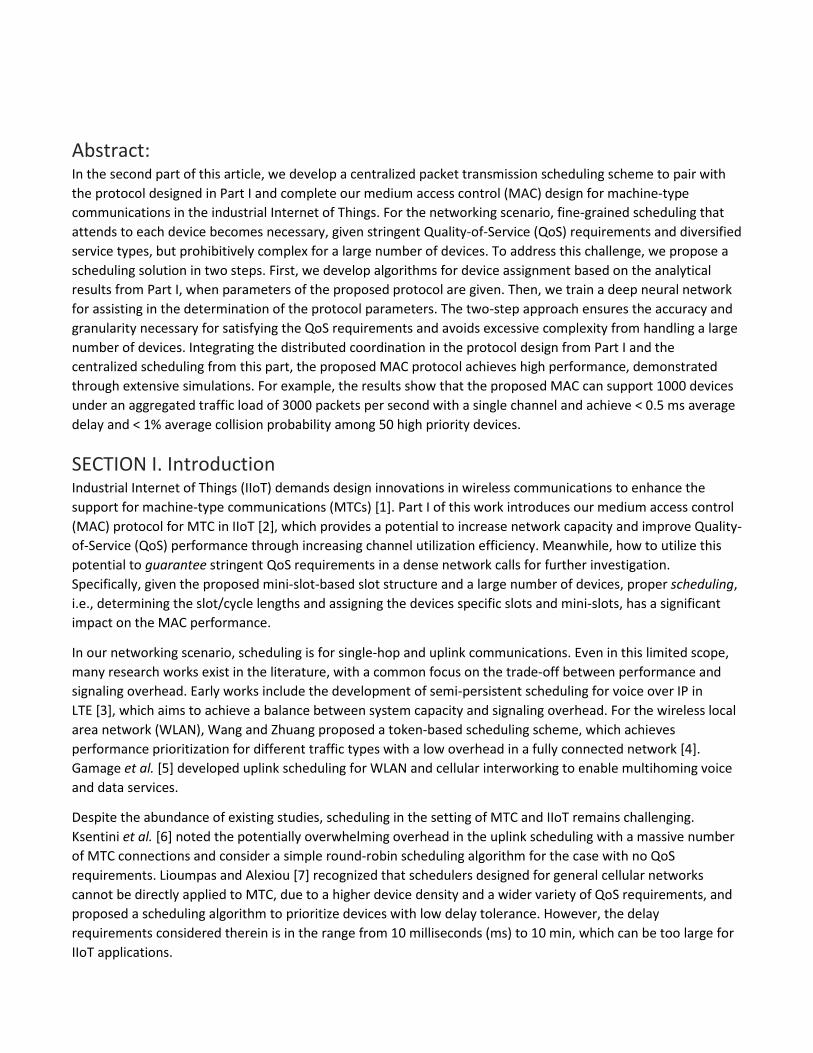
Abstract: In the second part of this article, we develop a centralized packet transmission scheduling scheme to pair with the protocol designed in Part I and complete our medium access control (MAC) design for machine-type communications in the industrial Internet of Things. For the networking scenario, fine-grained scheduling that attends to each device becomes necessary, given stringent Quality-of-Service (QoS) requirements and diversified service types, but prohibitively complex for a large number of devices. To address this challenge, we propose a scheduling solution in two steps. First, we develop algorithms for device assignment based on the analytical results from Part I, when parameters of the proposed protocol are given. Then, we train a deep neural network for assisting in the determination of the protocol parameters. The two-step approach ensures the accuracy and granularity necessary for satisfying the QoS requirements and avoids excessive complexity from handling a large number of devices. Integrating the distributed coordination in the protocol design from Part I and the centralized scheduling from this part, the proposed MAC protocol achieves high performance, demonstrated through extensive simulations. For example, the results show that the proposed MAC can support 1000 devices under an aggregated traffic load of 3000 packets per second with a single channel and achieve < 0.5 ms average delay and < 1% average collision probability among 50 high priority devices.

SECTION I. Introduction Industrial Internet of Things (IIoT) demands design innovations in wireless communications to enhance the support for machine-type communications (MTCs) [1]. Part I of this work introduces our medium access control (MAC) protocol for MTC in IIoT [2], which provides a potential to increase network capacity and improve Quality-of-Service (QoS) performance through increasing channel utilization efficiency. Meanwhile, how to utilize this potential to guarantee stringent QoS requirements in a dense network calls for further investigation. Specifically, given the proposed mini-slot-based slot structure and a large number of devices, proper scheduling, i.e., determining the slot/cycle lengths and assigning the devices specific slots and mini-slots, has a significant impact on the MAC performance.

In our networking scenario, scheduling is for single-hop and uplink communications. Even in this limited scope, many research works exist in the literature, with a common focus on the trade-off between performance and signaling overhead. Early works include the development of semi-persistent scheduling for voice over IP in LTE [3], which aims to achieve a balance between system capacity and signaling overhead. For the wireless local area network (WLAN), Wang and Zhuang proposed a token-based scheduling scheme, which achieves performance prioritization for different traffic types with a low overhead in a fully connected network [4]. Gamage et al. [5] developed uplink scheduling for WLAN and cellular interworking to enable multihoming voice and data services.

Despite the abundance of existing studies, scheduling in the setting of MTC and IIoT remains challenging. Ksentini et al. [6] noted the potentially overwhelming overhead in the uplink scheduling with a massive number of MTC connections and consider a simple round-robin scheduling algorithm for the case with no QoS requirements. Lioumpas and Alexiou [7] recognized that schedulers designed for general cellular networks cannot be directly applied to MTC, due to a higher device density and a wider variety of QoS requirements, and proposed a scheduling algorithm to prioritize devices with low delay tolerance. However, the delay requirements considered therein is in the range from 10 milliseconds (ms) to 10 min, which can be too large for IIoT applications.

To handle a large number of devices, a popular strategy is to divide the devices into groups (or clusters) and schedule the devices based on the groups [8]. Si et al. [9] proposed a grouping-based algorithm that adjusts the service rate for each user group to provide statistical QoS guarantees, where the considered delay requirements are in the range from 20 to 100 ms. Karadag et al. [10] presented semipersistent scheduling for MTC in cellular networks, taking delay constraints of devices into account, where devices have periodic traffic arrivals. Zhang et al. [11] proposed a random access scheme for MTC in cellular networks by grouping devices according to their delay requirements and applying access control for each group based on the group size, aggregated packet arrival rate, etc. Arouk et al. [12] proposed a group paging-based scheduling for massive MTC access in cellular networks, where the key idea is to scatter the contention for channel access to improve performance in terms of delay, collision probability, and energy consumption. The focuses of the last two works are on throughput maximization and energy consumption reduction, respectively, rather than supporting a stringent (e.g., ms level) delay requirement.

Given a high device density, diversified service types, and stringent QoS requirements, scheduling may need to be further fine-grained. Specifically, a scheduler may need to attend to the available information (e.g., packet arrival rate) or access strategy of each single device. Salodkar et al. [13] proposed a learning-assisted scheduling scheme, in which each device uses reinforcement learning to determine a preferred transmission rate and a base station (BS) schedules the device with the highest rate. Such a scheme can adapt to unknown packet arrival statistics. Chang et al. [14] proposed device-level uplink scheduling schemes based on conflict-avoiding codes, in which each device is assigned a 2D code matrix. These schemes are applicable when multiple channels are available. In their recent work, Rodoplu et al. [15] presented proactive forecasting-assisted scheduling to support massive access in the Internet of Things (IoT), which explores machine learning to predict the traffic of each device and reserve channel time accordingly. The scheme improves network performance with low overhead. Yang et al. [16] utilized a neural network to predict the number of IoT devices and Wi-Fi users, which facilitates dynamic scheduling and channel allocation for co-existing IoT and Wi-Fi communications.

In Part II of this work, our objective is to develop an effective scheduling scheme to pair with the proposed protocol in Part I. Different from the existing works, we focus on achieving QoS guarantee with very low delays. As a part of our MAC protocol, the scheduling scheme contributes to a customized link-layer solution to MTC in IIoT, supporting high device density, diversified service types, and stringent QoS targets. While we aim to maximize channel utilization efficiency through delicate distributed coordination in the MAC protocol in Part I, the focus of Part II is to develop a centralized analysis-based scheduling scheme. The scheduling scheme should achieve a desired balance in the QoS of different services or different QoS metrics for the same service. The integration of distributed coordination and centralized control is expected to strengthen the proposed MAC protocol.

With a large number of devices, finding a proper assignment for a centralized scheduler can be prohibitively complex. Scheduling for a dense network with hundreds or even thousands of devices can be beyond the reach of conventional approaches, when the packet arrival rate of each device may impact the protocol parameters and the QoS requirement of each device needs to be satisfied. This motivates us to exploit neural networks to assist scheduling. We propose to schedule in two steps, i.e., slot/mini-slot assignment and protocol parameter selection, and develop methods to reduce complexity in each step. The main contribution of this part is twofold: First, we develop algorithms to assign devices specific slots and mini-slots of the proposed protocol in Part I, when the protocol parameters are given. Based on the analytical results in Part I, the proposed algorithms sort devices of each type, estimate the impact of potential assignments for each device, and make assignments for the devices one by one. As a result, the assignments possess the due accuracy and granularity necessary for satisfying diverse and stringent QoS requirements; Second, to determine the protocol parameters, we exploit a deep neural network (DNN) to assist scheduling. The DNN is structured such that it can be used given any

number of devices and learn the mapping from various combinations of device and packet arrival profiles and protocol parameter settings to the resulting scheduling performance. We demonstrate that, after sufficient training, the DNN can learn the mapping. Then, given a specific device and packet arrival profile, the DNN can be used to compare different protocol parameter settings and determine proper parameters for the proposed MAC. In addition, we perform extensive simulations to demonstrate the properties of the proposed MAC protocol, the accuracy of the analysis in Part I, and the performance of the scheduling scheme developed in this part.

The remainder of Part II is organized as follows. Section II describes the scheduling problem. Section III investigates the device assignment. In Section IV, we exploit a DNN to determine protocol parameters. Section V present the numerical results, and Section VI concludes this work.

SECTION II. Scheduling Problem Our considered network scenario and proposed MAC protocol are given in Sections II and III of Part I, respectively [2]. To avoid redundancy, we refer readers to the aforementioned sections for the related information. According to the protocol description in Section III and performance analysis in Section IV in Part I of this article, it is clear that the following factors have significant impact on the performance of the proposed MAC protocol.

1. The number of mini-slots in each slot, i.e., 𝑛𝑛m.

2. The assignment cycles 𝑟𝑟H, 𝑟𝑟R, and 𝑟𝑟L, which serve as different frame lengths for different types of devices.

3. The device assignment, i.e., the allocation of devices to slots and mini-slots.

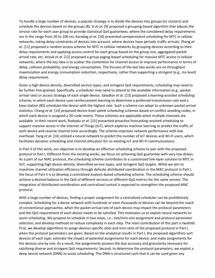
We refer to the problem of determining the above factors with the objective of satisfying QoS requirements as the packet transmission scheduling problem, which is illustrated in Fig. 1. The access point (AP) in the network is expected to have computing capability and conduct the scheduling.

Fig. 1. Illustration of the scheduling problem. Different colors in the sub-blocks of a mini-slot correspond to different devices assigned that mini-slot, while dot-filled, solid-filled, and grid-filled patterns represent mini-slots assigned to high-priority (HP), regular-priority (RP), and low-priority (LP) devices, respectively. The scheduling problem involves determining protocol parameters 𝑛𝑛m, 𝑟𝑟H, 𝑟𝑟R, and 𝑟𝑟L as well as assigning slots and mini-slots to all devices.

Note that the scheduling problem may not always be feasible. Indeed, we cannot guarantee the satisfaction of arbitrary QoS requirements given an arbitrarily large set of devices with arbitrary packet arrival rates. Thus, the objective here is to investigate effective scheduling that can support as many devices as possible while satisfying their QoS requirements.

Given the sets of all devices 𝒟𝒟 = {1, … ,𝐷𝐷}, HP devices 𝒟𝒟H, RP devices 𝒟𝒟R, LP devices 𝒟𝒟L, and packet arrival rates {𝜆𝜆𝑖𝑖}, 𝑖𝑖 ∈ 𝒟𝒟, we attempt to accommodate all devices while satisfying the delay requirements 𝛿𝛿H, 𝛿𝛿R, and 𝛿𝛿L and packet collision probability requirements 𝜌𝜌H, 𝜌𝜌R, and 𝜌𝜌L for the HP, RP, and LP devices, respectively. Based on the protocol, the following constraints exist for the scheduling problem (see Section III-D of Part I).

1. The LP assignment cycle length 𝑟𝑟L is a multiple of the RP assignment cycle length 𝑟𝑟R, which in turn is a multiple of the HP assignment cycle length 𝑟𝑟H.

2. A mini-slot should not accommodate more than one type of devices.

3. If mini-slot 𝑚𝑚 of slot 𝑙𝑙, where 𝑙𝑙 ≤ 𝑟𝑟H and 𝑚𝑚 ≤ 𝑛𝑛m, is assigned to a subset of HP devices ℐH, then mini-slot 𝑚𝑚 of slot 𝑙𝑙′, for any 𝑙𝑙′ ∈ {𝑟𝑟H + 𝑙𝑙, 2𝑟𝑟H + 𝑙𝑙, … , 𝑟𝑟L − 𝑟𝑟H + 𝑙𝑙}, is also assigned to the same set of HP devices ℐH. If mini-slot 𝑚𝑚 of slot 𝑙𝑙, where 𝑙𝑙 ≤ 𝑟𝑟R and 𝑚𝑚 ≤ 𝑛𝑛m, is assigned to a subset of RP devices ℐR, then mini-slot 𝑚𝑚 of 𝑙𝑙′, for any 𝑙𝑙′ ∈ {𝑟𝑟R + 𝑙𝑙, 2𝑟𝑟R + 𝑙𝑙, … , 𝑟𝑟L − 𝑟𝑟R + 𝑙𝑙}, is also assigned to the same set of RP devices ℐR. Both cases are illustrated in illustrated in Fig. 1.

To solve the scheduling problem, we first investigate the device assignment while assuming the protocol parameters 𝑛𝑛m, 𝑟𝑟H, 𝑟𝑟R, and 𝑟𝑟L are given. Then, we explore a DNN to assist determining these parameters. In both steps, we assume that mini-slot-based carrier sensing (MsCS), synchronization carrier sensing (SyncCS), differentiated assignment cycles, and superimposed mini-slot assignment (SMsA) from Part I are all adopted in the proposed MAC protocol.

SECTION III. Device Assignment In this section, we first discuss the impact of protocol parameters (𝑛𝑛m, 𝑟𝑟H, 𝑟𝑟R, and 𝑟𝑟L) and then investigate the device assignment problem.

A. Impact of 𝑛𝑛m Intuitively, increasing 𝑛𝑛m, subject to the conditions mentioned in the end of Section III-B of Part I, can support more devices via more mini-slots. However, increasing 𝑛𝑛m increases delay, and consequently packet collision probability, of all devices. Therefore, given the QoS requirements of devices, increasing 𝑛𝑛m may reduce the number of supported devices subject to the requirements.

B. Impact of 𝑟𝑟H, 𝑟𝑟R, and 𝑟𝑟L The delay requirements 𝛿𝛿H, 𝛿𝛿R, 𝛿𝛿L place constraints on 𝑟𝑟H, 𝑟𝑟R, and 𝑟𝑟L, respectively. Consider HP devices for example. When there are 𝑛𝑛m mini-slots in each slot, an upper bound on the number of slots per HP assignment cycle, i.e., 𝑟𝑟H, is given by1

𝑟𝑟H = �2𝛿𝛿H

𝑛𝑛m𝑇𝑇m + 𝑇𝑇x�

(1)

where ⌊⋅⌋ is the floor function. The denominator is the length of a slot. The factor “2” in the numerator follows from the fact that the average gap between the beginning of an HP cycle and the arrival of an HP packet is equal to one half of an HP cycle.

Using (1), a relation between 𝑛𝑛m and 𝑟𝑟H can be obtained. If 𝑛𝑛m is large, 𝑟𝑟H should be small, and the HP devices will be “densely” packed into the 𝑟𝑟H slots. As a result, it can be challenging to satisfy the QoS requirements of HP devices. On the other hand, if 𝑛𝑛m is small so that 𝑟𝑟H can become large, more slots are available for HP devices in each frame. However, the transmission opportunity for RP and LP devices will decrease. Therefore, determining appropriate values for 𝑟𝑟H, 𝑟𝑟R, and 𝑟𝑟L is crucial but nontrivial.

C. Device Assignment The assignment of slots and mini-slots to devices is a complex problem. Consider the case with buffer and SMsA. Even if 𝑛𝑛m, 𝑟𝑟H, 𝑟𝑟R, and 𝑟𝑟L are given, the device assignment is a combinatorial integer programming problem. Based on the analysis in Section IV-E of Part I, assigning any new device an occupied mini-slot can affect the delay and collision probability of all other devices assigned that mini-slot.

We propose a heuristic algorithm for device assignment, built on the analysis in Section IV of Part I, when 𝑛𝑛m, 𝑟𝑟H, 𝑟𝑟R, and 𝑟𝑟L are given. The analysis allows us to estimate the delay and collision probability of devices in a mini-slot after adding each new device to the mini-slot. The proposed assignment algorithm tentatively assigns a device while estimating the resulting performance, with the target of satisfying the QoS requirements of all assigned devices in the process. The following settings are used in the assignment.

1. All devices assigned the same mini-slot have the same priority type.

2. The maximum packet collision probability among all devices assigned the same mini-slot is referred to as the collision probability for that mini-slot and denoted by 𝑞𝑞𝑚𝑚,𝑙𝑙

c for mini-slot 𝑚𝑚 of slot 𝑙𝑙.

3. Under the assumption that the impact of collision probability on the cycle length is negligible, the length of an LP cycle can be calculated by

𝑇𝑇fL =𝑟𝑟L𝑛𝑛m𝑇𝑇𝑚𝑚

1 − ∑ 𝜆𝜆𝑖𝑖𝑇𝑇x𝑖𝑖∈𝒟𝒟

(2)

which is based on (12) in Part I of this article. The parameter ns in (12) of Part I, i.e., the number of slots in a general frame, is replaced with 𝑟𝑟L in (2) since an LP cycle serves as a frame for LP devices. Note that the use of differentiated assignment cycles does not change the packet arrival rates. Based on the constraints mentioned in Section II, all devices should be scheduled at least once in an LP cycle, which leads to the summation over the packet arrival rates of all devices in the denominator of (2).

Let 𝑚𝑚^𝑙𝑙 denote the minimum index among the mini-slots of slot l that have not been assigned to any device. For

notation simplicity, we omit subscript 𝑙𝑙 in 𝑚𝑚^𝑙𝑙 when 𝑚𝑚

^𝑙𝑙 and 𝑙𝑙 both appear in the subscript (e.g., 𝑞𝑞

𝑚𝑚^𝑙𝑙,𝑙𝑙

c will be

written as 𝑞𝑞𝑚𝑚^

,𝑙𝑙c ). The length of the HP, RP, and LP assignment cycles are denoted by 𝑇𝑇fH,𝑇𝑇fR, and 𝑇𝑇fL, respectively.

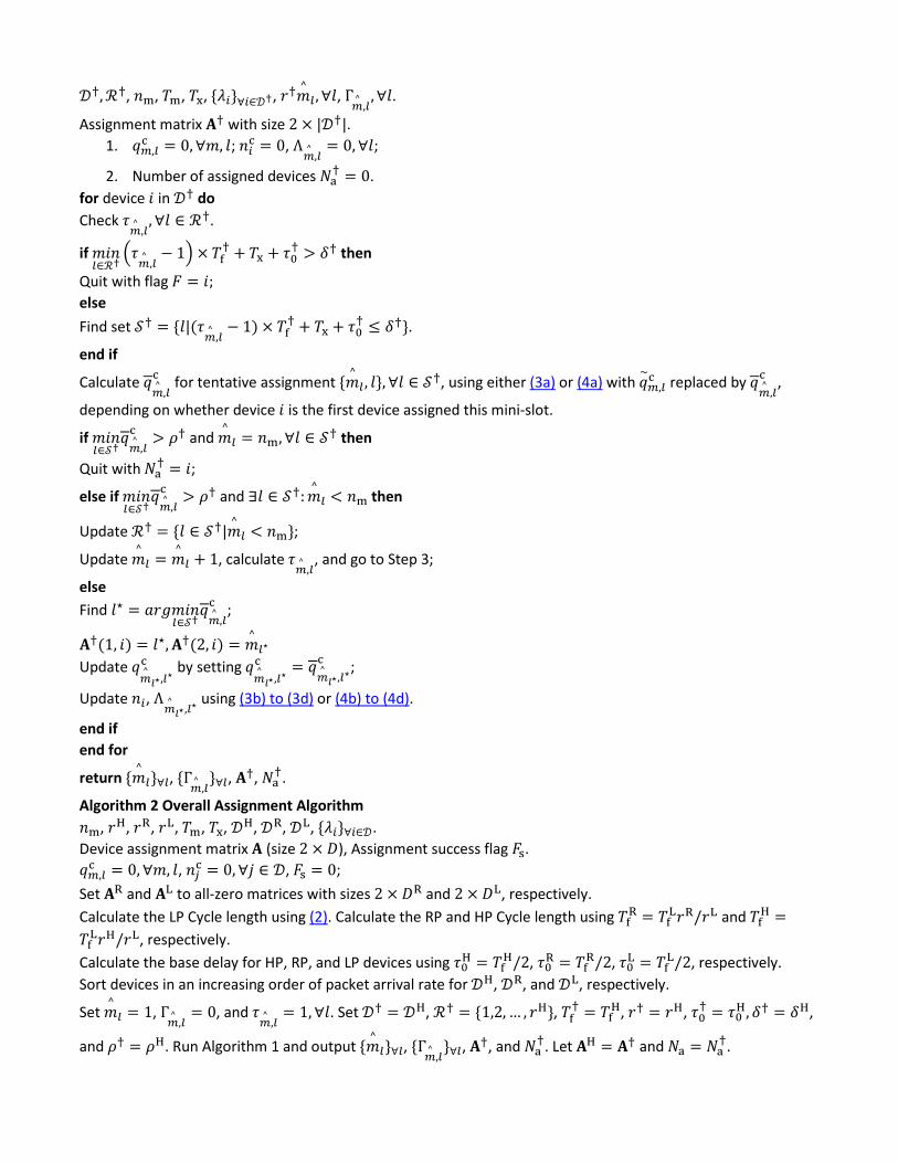
The proposed assignment is given in Algorithms 1 and 2. Algorithm 1 is the core algorithm for assigning slots and mini-slots to a set of devices with the same priority for a given cycle length, while Algorithm 2 is the overall algorithm that calls Algorithm 1 to make assignments for all devices and all cycles.

Algorithm 1 Core Assignment Algorithm

𝒟𝒟†,ℛ†, 𝑛𝑛m, 𝑇𝑇m, 𝑇𝑇x, {𝜆𝜆𝑖𝑖}∀𝑖𝑖∈𝒟𝒟†, 𝑟𝑟†𝑚𝑚^𝑙𝑙 ,∀𝑙𝑙, Γ𝑚𝑚^ ,𝑙𝑙

,∀𝑙𝑙.

Assignment matrix 𝐀𝐀† with size 2 × |𝒟𝒟†|. 1. 𝑞𝑞𝑚𝑚,𝑙𝑙

c = 0,∀𝑚𝑚, 𝑙𝑙; 𝑛𝑛𝑖𝑖c = 0, Λ𝑚𝑚^

,𝑙𝑙= 0,∀𝑙𝑙;

2. Number of assigned devices 𝑁𝑁a† = 0.

for device 𝑖𝑖 in 𝒟𝒟† do Check 𝜏𝜏

𝑚𝑚^

,𝑙𝑙,∀𝑙𝑙 ∈ ℛ†.

if 𝑚𝑚𝑖𝑖𝑛𝑛𝑙𝑙∈ℛ†

�𝜏𝜏𝑚𝑚^

,𝑙𝑙− 1� × 𝑇𝑇f

† + 𝑇𝑇x + 𝜏𝜏0† > 𝛿𝛿† then

Quit with flag 𝐹𝐹 = 𝑖𝑖; else Find set 𝒮𝒮† = {𝑙𝑙|(𝜏𝜏

𝑚𝑚^

,𝑙𝑙− 1) × 𝑇𝑇f

† + 𝑇𝑇x + 𝜏𝜏0† ≤ 𝛿𝛿†}.

end if

Calculate 𝑞𝑞𝑚𝑚^

,𝑙𝑙c for tentative assignment {𝑚𝑚

^𝑙𝑙 , 𝑙𝑙},∀𝑙𝑙 ∈ 𝒮𝒮†, using either (3a) or (4a) with 𝑞𝑞

~𝑚𝑚,𝑙𝑙c replaced by 𝑞𝑞

𝑚𝑚^

,𝑙𝑙c ,

depending on whether device 𝑖𝑖 is the first device assigned this mini-slot.

if 𝑚𝑚𝑖𝑖𝑛𝑛𝑙𝑙∈𝒮𝒮†

𝑞𝑞𝑚𝑚^

,𝑙𝑙c > 𝜌𝜌† and 𝑚𝑚

^𝑙𝑙 = 𝑛𝑛m,∀𝑙𝑙 ∈ 𝒮𝒮† then

Quit with 𝑁𝑁a† = 𝑖𝑖;

else if 𝑚𝑚𝑖𝑖𝑛𝑛𝑙𝑙∈𝒮𝒮†

𝑞𝑞𝑚𝑚^

,𝑙𝑙c > 𝜌𝜌† and ∃𝑙𝑙 ∈ 𝒮𝒮†:𝑚𝑚

^𝑙𝑙 < 𝑛𝑛m then

Update ℛ† = {𝑙𝑙 ∈ 𝒮𝒮†|𝑚𝑚^𝑙𝑙 < 𝑛𝑛m};

Update 𝑚𝑚^𝑙𝑙 = 𝑚𝑚

^𝑙𝑙 + 1, calculate 𝜏𝜏

𝑚𝑚^

,𝑙𝑙, and go to Step 3;

else Find 𝑙𝑙⋆ = 𝑎𝑎𝑟𝑟𝑎𝑎𝑚𝑚𝑖𝑖𝑛𝑛

𝑙𝑙∈𝒮𝒮†𝑞𝑞𝑚𝑚^

,𝑙𝑙c ;

𝐀𝐀†(1, 𝑖𝑖) = 𝑙𝑙⋆,𝐀𝐀†(2, 𝑖𝑖) = 𝑚𝑚^𝑙𝑙⋆

Update 𝑞𝑞𝑚𝑚^𝑙𝑙⋆ ,𝑙𝑙⋆

c by setting 𝑞𝑞𝑚𝑚^𝑙𝑙⋆ ,𝑙𝑙⋆

c = 𝑞𝑞𝑚𝑚^𝑙𝑙⋆ ,𝑙𝑙⋆

c ;

Update 𝑛𝑛𝑖𝑖, Λ𝑚𝑚^ 𝑙𝑙⋆ ,𝑙𝑙⋆ using (3b) to (3d) or (4b) to (4d).

end if end for

return {𝑚𝑚^𝑙𝑙}∀𝑙𝑙, {Γ𝑚𝑚^ ,𝑙𝑙

}∀𝑙𝑙, 𝐀𝐀†, 𝑁𝑁a†.

Algorithm 2 Overall Assignment Algorithm 𝑛𝑛m, 𝑟𝑟H, 𝑟𝑟R, 𝑟𝑟L, 𝑇𝑇m, 𝑇𝑇x, 𝒟𝒟H, 𝒟𝒟R, 𝒟𝒟L, {𝜆𝜆𝑖𝑖}∀𝑖𝑖∈𝒟𝒟. Device assignment matrix 𝐀𝐀 (size 2 × 𝐷𝐷), Assignment success flag 𝐹𝐹s. 𝑞𝑞𝑚𝑚,𝑙𝑙c = 0,∀𝑚𝑚, 𝑙𝑙, 𝑛𝑛𝑗𝑗c = 0,∀𝑗𝑗 ∈ 𝒟𝒟, 𝐹𝐹s = 0;

Set 𝐀𝐀R and 𝐀𝐀L to all-zero matrices with sizes 2 × 𝐷𝐷R and 2 × 𝐷𝐷L, respectively. Calculate the LP Cycle length using (2). Calculate the RP and HP Cycle length using 𝑇𝑇fR = 𝑇𝑇fL𝑟𝑟R/𝑟𝑟L and 𝑇𝑇fH =𝑇𝑇fL𝑟𝑟H/𝑟𝑟L, respectively. Calculate the base delay for HP, RP, and LP devices using 𝜏𝜏0H = 𝑇𝑇fH/2, 𝜏𝜏0R = 𝑇𝑇fR/2, 𝜏𝜏0L = 𝑇𝑇fL/2, respectively. Sort devices in an increasing order of packet arrival rate for 𝒟𝒟H, 𝒟𝒟R, and 𝒟𝒟L, respectively.

Set 𝑚𝑚^𝑙𝑙 = 1, Γ

𝑚𝑚^

,𝑙𝑙= 0, and 𝜏𝜏

𝑚𝑚^

,𝑙𝑙= 1,∀𝑙𝑙. Set 𝒟𝒟† = 𝒟𝒟H, ℛ† = {1,2, … , 𝑟𝑟H}, 𝑇𝑇f

† = 𝑇𝑇fH, 𝑟𝑟† = 𝑟𝑟H, 𝜏𝜏0† = 𝜏𝜏0H, 𝛿𝛿† = 𝛿𝛿H,

and 𝜌𝜌† = 𝜌𝜌H. Run Algorithm 1 and output {𝑚𝑚^𝑙𝑙}∀𝑙𝑙, {Γ𝑚𝑚^ ,𝑙𝑙

}∀𝑙𝑙, 𝐀𝐀†, and 𝑁𝑁a†. Let 𝐀𝐀H = 𝐀𝐀† and 𝑁𝑁a = 𝑁𝑁a

†.

if 𝑁𝑁aH = |𝒟𝒟H| then

Update 𝑚𝑚^𝑙𝑙 = 𝑚𝑚

^𝑙𝑙 + 1,∀𝑙𝑙; Update ℛ† = {𝑙𝑙|𝑙𝑙 ∈ [1, 𝑟𝑟R],𝑚𝑚

^𝑙𝑙 ≤ 𝑛𝑛m}; For each slot 𝑙𝑙 ∈ ℛ† and any 𝑙𝑙′ ∈ {𝑟𝑟H +

𝑙𝑙, 2𝑟𝑟H + 𝑙𝑙, … , 𝑟𝑟R − 𝑟𝑟H + 𝑙𝑙}, add 𝑙𝑙′ to ℛ† and let Γ𝑚𝑚^

,𝑙𝑙′ equal Γ

𝑚𝑚^

,𝑙𝑙. Then, calculate 𝜏𝜏

𝑚𝑚^

,𝑙𝑙,∀𝑙𝑙 ∈ ℛ†.

Run Algorithm 1 with inputs {Γ𝑚𝑚^

,𝑙𝑙}∀𝑙𝑙 and 𝑟𝑟† from Step 2, 𝒟𝒟† = 𝒟𝒟R, 𝑇𝑇f

† = 𝑇𝑇fR, 𝑟𝑟† = 𝑟𝑟R, 𝜏𝜏0† = 𝜏𝜏0R, 𝛿𝛿† = 𝛿𝛿R, 𝜌𝜌† =

𝜌𝜌R. Obtain output {𝑚𝑚^𝑙𝑙}∀𝑙𝑙, {Γ𝑚𝑚^ ,𝑙𝑙

}∀𝑙𝑙, 𝐀𝐀†, and 𝑁𝑁a†. Let 𝐀𝐀R = 𝐀𝐀† and 𝑁𝑁a = 𝑁𝑁a + 𝑁𝑁a

†.

if 𝑁𝑁a† = |𝒟𝒟R| then

Update 𝑚𝑚^𝑙𝑙 = 𝑚𝑚

^𝑙𝑙 + 1,∀𝑙𝑙; Update ℛ† = {𝑙𝑙|𝑙𝑙 ∈ [1, 𝑟𝑟L],𝑚𝑚

^𝑙𝑙 ≤ 𝑛𝑛s}; For each slot 𝑙𝑙 ∈ ℛ† and any 𝑙𝑙′ ∈ {𝑟𝑟R + 𝑙𝑙, 2𝑟𝑟R +

𝑙𝑙, … , 𝑟𝑟L − 𝑟𝑟R + 𝑙𝑙}, add 𝑙𝑙′ to 𝑟𝑟† and let Γ𝑚𝑚^

,𝑙𝑙′ equal Γ

𝑚𝑚^

,𝑙𝑙. Then, calculate 𝜏𝜏

𝑚𝑚^

,𝑙𝑙,∀𝑙𝑙 ∈ ℛ†.

Run Algorithm 1 with inputs {Γ𝑚𝑚^

,𝑙𝑙}∀𝑙𝑙 and 𝑟𝑟† from Step 2, 𝒟𝒟† = 𝒟𝒟L, 𝑇𝑇f

† = 𝑇𝑇fL, 𝑟𝑟† = 𝑟𝑟L, 𝜏𝜏0† = 𝜏𝜏0L, 𝛿𝛿† = 𝛿𝛿L, 𝜌𝜌† =

𝜌𝜌L. Obtain output 𝐀𝐀†, and 𝑁𝑁a†. Let 𝐀𝐀L = 𝐀𝐀† and 𝑁𝑁a = 𝑁𝑁a +𝑁𝑁a

†. Set 𝐹𝐹s = 1 if 𝑁𝑁a = 𝐷𝐷. end if end if return 𝐀𝐀 = [𝐀𝐀H,𝐀𝐀R,𝐀𝐀L], 𝐹𝐹s.

In the two algorithms, variables 𝑛𝑛𝑖𝑖c, Λ𝑚𝑚,𝑙𝑙, and Γ𝑚𝑚,𝑙𝑙 denote the expected number of simultaneously transmitting packets given that device 𝑖𝑖 is transmitting (which can be larger than 1 as a result of a nonzero collision probability), the aggregated packet arrival rate for all devices assigned mini-slot 𝑚𝑚 of slot 𝑙𝑙, and the accumulated number of packet arrivals for all devices assigned mini-slots 1 to m of slot l in the corresponding cycle, respectively. Detailed description can be found in Appendix C of Part I and is omitted here for brevity.

The basic ideas of Algorithms 1 and 2 are given as follows. Algorithm 1 assigns mini-slots to devices, starting from the first mini-slot of every slot, and tracks the current mini-slot being assigned. It tentatively assigns a device the current mini-slot of all available slots, trying to find the best assignment based on the resulting delay and packet collision probability estimations. If the current mini-slot in none of the slots can accommodate the device by satisfying its collision probability requirement, the algorithm moves to the next mini-slot. The procedure repeats until any of the following three conditions is satisfied: 1) all devices are allocated; 2) there is no more vacant mini-slot; or 3) no current mini-slot can satisfy the delay requirement of a device. Algorithm 2 sorts the devices and calls Algorithm 1 for mini-slot and slot assignment for each device priority type. After obtaining an assignment for HP devices and RP devices, Algorithm 2 extends the assignment for the RP cycle and LP cycle, respectively. Some details of main steps in the algorithms are summarized as follows.

1. Step 3 of Algorithm 1: The left-hand side of the inequality represents the overall delay including the base and access delays. The calculation is discussed in Section IV-A of Part I.

2. Step 1 of Algorithm 1 and Steps 2 and 2 of Algorithm 2: These steps move from the current mini-slot to the next mini-slot of the same slot. As a result, the access delay counted in frames (AD-F) of the next mini-slot needs to be calculated. The calculation of 𝜏𝜏

𝑚𝑚^

,𝑙𝑙 in these steps is based on (34) in Part I

with 𝑇𝑇f replaced by the corresponding HP, RP, or LP cycle length.

3. Step 2 of Algorithm 2: Since each LP assignment cycle consists of 𝑟𝑟L/𝑟𝑟H HP cycles and 𝑟𝑟L/𝑟𝑟R RP cycles, respectively, the HP and RP assignment cycles can be found accordingly after obtaining the LP cycle length based on (2).

4. Step 2 of Algorithm 2: The element in the first/second row and the 𝑖𝑖 th column of the device assignment matrix 𝐀𝐀 gives the index of the slot/mini-slot assigned to device 𝑖𝑖.

5. Matrix A only gives the first slot/mini-slot assigned to device i. If device i is an HP device and assigned slot and mini-slot {𝑙𝑙,𝑚𝑚}, then it is also assigned slot/mini-slot {𝑙𝑙′,𝑚𝑚} for any 𝑙𝑙′ ∈ {𝑟𝑟H + 𝑙𝑙, 2𝑟𝑟H +𝑙𝑙, … , 𝑟𝑟L − 𝑟𝑟H + 𝑙𝑙}. If device 𝑖𝑖 is an RP device and assigned slot and mini-slot {𝑙𝑙,𝑚𝑚}, then it is also assigned slot/mini-slot any 𝑙𝑙′ ∈ {𝑟𝑟R + 𝑙𝑙, 2𝑟𝑟R + 𝑙𝑙, … , 𝑟𝑟L − 𝑟𝑟R + 𝑙𝑙}. This is reflected in steps 2 and 2 of Algorithm 2 and consistent with the illustration in Fig. 1.

In the core assignment algorithm (Algorithm 1), adding a device to a mini-slot has an impact on Λ𝑚𝑚,𝑙𝑙, Γ𝑚𝑚,𝑙𝑙, and 𝑞𝑞𝑚𝑚,𝑙𝑙

c . Therefore, after assigning device 𝑖𝑖 mini-slot 𝑚𝑚 of slot 𝑙𝑙, these variables need to be updated for the mini-slot. If device 𝑖𝑖 is the first device assigned mini-slot 𝑚𝑚 of slot 𝑙𝑙, the following update applies:

𝑞𝑞~𝑚𝑚,𝑙𝑙c = 0𝑛𝑛~𝑖𝑖 = 1

Λ~𝑚𝑚,𝑙𝑙 = 𝜆𝜆𝑖𝑖Γ~𝑚𝑚,𝑙𝑙 = Γ𝑚𝑚,𝑙𝑙 + 𝑇𝑇f

†𝜆𝜆𝑖𝑖𝜏𝜏~𝑚𝑚,𝑙𝑙 = 𝜏𝜏𝑚𝑚,𝑙𝑙

(3a)(3b)(3c)(3d)(3e)

where 𝑥𝑥~

represents an updated value of x after assigning device 𝑖𝑖, and 𝑇𝑇f† is the corresponding (HP, RP, or LP)

cycle length. If device 𝑖𝑖 is not the first device assigned mini-slot 𝑚𝑚 of slot 𝑙𝑙, the following update applies:

𝑞𝑞~𝑚𝑚,𝑙𝑙c = �1 − �1 − 𝑞𝑞𝑚𝑚,𝑙𝑙

c ��1− 𝑇𝑇f†𝜆𝜆𝑖𝑖��

𝑛𝑛𝑖𝑖c = 1 + � 𝜏𝜏𝑚𝑚,𝑙𝑙𝑇𝑇f†𝜆𝜆𝑗𝑗

𝑗𝑗∈𝒟𝒟𝑚𝑚,𝑙𝑙∖{𝑖𝑖}

Λ~𝑚𝑚,𝑙𝑙 = Λ𝑚𝑚,𝑙𝑙 + 𝜆𝜆𝑖𝑖 �1 −

𝑞𝑞~𝑚𝑚,𝑙𝑙c

𝑛𝑛𝑖𝑖c�

Γ~𝑚𝑚,𝑙𝑙 = Γ𝑚𝑚,𝑙𝑙 + 𝑇𝑇f

†𝜆𝜆𝑖𝑖 �1 −𝑞𝑞~𝑚𝑚,𝑙𝑙c

𝑛𝑛𝑖𝑖c�

𝜏𝜏~𝑚𝑚,𝑙𝑙 = 𝜏𝜏𝑚𝑚,𝑙𝑙

(4a)(4b)(4c)(4d)(4e)

which is based on the analysis in Section IV-E of Part I. Equations (4a)–(4d) update the packet collision probability,2 the average number of packets per transmission (taking collision into account), the aggregated packet arrival rate, and the accumulated number of packet arrivals, respectively, corresponding to a mini-slot after a new device is assigned that mini-slot. The last equation, i.e., (4e), follows from the proof of Theorem 3 in Part I. Specifically, the result (34) in Part I shows that, under a low collision probability, the AD-F for devices assigned any mini-slot depends on the packet arrival rates of all devices in the preceding mini-slots, but not the packet arrival rates of other devices sharing the same mini-slot.

SECTION IV. Learning-Assisted Scheduling The proposed device assignment in the preceding section can be applied when the parameters 𝑛𝑛m, 𝑟𝑟H, 𝑟𝑟R, and 𝑟𝑟L are given. In this section, we propose learning-assisted scheduling to determine the values of these protocol parameters.

A. Motivation for Learning-Assisted Scheduling Choosing proper values for those protocol parameters is challenging. First, the impact of protocol parameters 𝑛𝑛m, 𝑟𝑟H, 𝑟𝑟R, 𝑟𝑟L and the impact of device assignment are correlated. For example, knowledge of the slot/mini-slot assignment is required to analyze the impact of 𝑛𝑛m, while the assignment cannot be determined without knowing 𝑛𝑛m first. Second, the effects of 𝑛𝑛m, 𝑟𝑟H, 𝑟𝑟R, 𝑟𝑟L on the performance are mutually dependent. Consider 𝑛𝑛m and 𝑟𝑟H as an example. Both 𝑛𝑛m and 𝑟𝑟H affect the delay of HP devices. The impact of adjusting 𝑟𝑟H depends on the value of 𝑛𝑛m, and the dependence is further affected by the device packet arrival rate profile. As a result, we cannot establish an analytical model for 𝑛𝑛m, 𝑟𝑟H, 𝑟𝑟R, and 𝑟𝑟L. On the other hand, using brutal force to choose their values is not viable due to the large number of diverse devices. There are usually too many candidate combinations of 𝑛𝑛m, 𝑟𝑟H, 𝑟𝑟R, and 𝑟𝑟L, and each combination requires a recalculation of the device assignment using Algorithms 1 and 2. As the assignment algorithm is based on calculating the delay and collision probability while assigning each device, the complexity of recalculating all assignment for all combinations can be very high.3

Consequently, we use a learning-based method to capture the impact of 𝑛𝑛m, 𝑟𝑟H, 𝑟𝑟R, 𝑟𝑟L and determine their values. Specifically, we train a DNN to learn the mapping from the combination of device and packet arrival rate profiles and protocol parameter settings to the protocol performance. A significant part of the training can be done offline to avoid a long training duration in an online setting caused by searching for and determining appropriate protocol parameters.

B. Role of the DNN We use a DNN to assist the AP in determining the parameters of the proposed MAC protocol, as follows. First, for each device and packet arrival rate profile,4 we try different combinations of 𝑛𝑛m, 𝑟𝑟H, 𝑟𝑟R, and 𝑟𝑟L, use the heuristic algorithm to obtain the assignment, and test the resulting performance using simulations. Then, the device and packet arrival rate profile, protocol parameter settings (𝑛𝑛m, 𝑟𝑟H, 𝑟𝑟R, and 𝑟𝑟L), and the resulting protocol performance (as label) are used to train and test the DNN.

The data generation, training, and testing are conducted offline. When the DNN is well-trained, we can imitate the mapping from a device and packet arrival rate profile and a protocol parameter setting to the protocol performance. Accordingly, we can determine the protocol parameters online by trying different parameters on the DNN and compare the resulting performance. Recall that the packet arrival rates of devices remain constant in a relatively long duration, as mentioned in Part I. When an update of the packet arrival rates occurs, it triggers a decision on the protocol parameters, and the DNN assists the decision making as aforementioned.

Specifically, the DNN works as follows. The input of the DNN includes the following two components.

1. Device and packet arrival rate profile—to be flexible with the number of devices, we divide the range of packet arrival rate into 𝐼𝐼 intervals. Letting 𝜆𝜆𝑚𝑚𝑚𝑚𝑚𝑚 and 𝜆𝜆𝑚𝑚𝑖𝑖𝑚𝑚 denote the maximum and minimum packet arrival rates, the width of each interval is (𝜆𝜆𝑚𝑚𝑚𝑚𝑚𝑚 − 𝜆𝜆𝑚𝑚𝑖𝑖𝑚𝑚)/𝐼𝐼. We count the number of HP, RP, and LP devices in each of the 𝐼𝐼 intervals and organize the corresponding numbers into three 𝐼𝐼 ×1 vectors 𝐜𝐜H, 𝐜𝐜R, and 𝐜𝐜L, respectively.

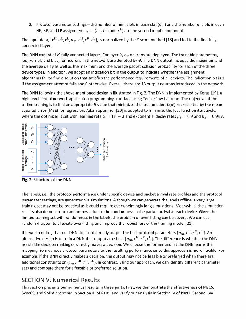
2. Protocol parameter settings—the number of mini-slots in each slot (𝑛𝑛m) and the number of slots in each HP, RP, and LP assignment cycle (𝑟𝑟H, 𝑟𝑟R, and 𝑟𝑟L) are the second input component.

The input data, {𝐜𝐜H, 𝐜𝐜R, 𝐜𝐜L,𝑛𝑛m, 𝑟𝑟H, 𝑟𝑟R, 𝑟𝑟L}, is normalized by the Z-score method [18] and fed to the first fully connected layer.

The DNN consist of 𝐾𝐾 fully connected layers. For layer 𝑘𝑘, 𝑛𝑛𝑘𝑘 neurons are deployed. The trainable parameters, i.e., kernels and bias, for neurons in the network are denoted by 𝜽𝜽. The DNN output includes the maximum and the average delay as well as the maximum and the average packet collision probability for each of the three device types. In addition, we adopt an indication bit in the output to indicate whether the assignment algorithms fail to find a solution that satisfies the performance requirements of all devices. The indication bit is 1 if the assignment attempt fails and 0 otherwise. Overall, there are 13 output neurons introduced in the network.

The DNN following the above-mentioned design is illustrated in Fig. 2. The DNN is implemented by Keras [19], a high-level neural network application programming interface using Tensorflow backend. The objective of the offline training is to find an appropriate 𝜽𝜽 value that minimizes the loss function ℒ(𝜽𝜽) represented by the mean squared error (MSE) for regression. Adam optimizer [20] is adopted to minimize the loss function iteratively, where the optimizer is set with learning rate 𝛼𝛼 = 1𝑒𝑒 − 3 and exponential decay rates 𝛽𝛽1 = 0.9 and 𝛽𝛽2 = 0.999.

Fig. 2. Structure of the DNN.

The labels, i.e., the protocol performance under specific device and packet arrival rate profiles and the protocol parameter settings, are generated via simulations. Although we can generate the labels offline, a very large training set may not be practical as it could require overwhelmingly long simulations. Meanwhile, the simulation results also demonstrate randomness, due to the randomness in the packet arrival at each device. Given the limited training set with randomness in the labels, the problem of over-fitting can be severe. We can use random dropout to alleviate over-fitting and improve the robustness of the training model [21].

It is worth noting that our DNN does not directly output the best protocol parameters {𝑛𝑛m, 𝑟𝑟H, 𝑟𝑟R, 𝑟𝑟L}. An alternative design is to train a DNN that outputs the best {𝑛𝑛m, 𝑟𝑟H, 𝑟𝑟R, 𝑟𝑟L}. The difference is whether the DNN assists the decision making or directly makes a decision. We choose the former and let the DNN learns the mapping from various protocol parameters to the resulting performance since this approach is more flexible. For example, if the DNN directly makes a decision, the output may not be feasible or preferred when there are additional constraints on {𝑛𝑛m, 𝑟𝑟H, 𝑟𝑟R, 𝑟𝑟L}. In contrast, using our approach, we can identify different parameter sets and compare them for a feasible or preferred solution.

SECTION V. Numerical Results This section presents our numerical results in three parts. First, we demonstrate the effectiveness of MsCS, SyncCS, and SMsA proposed in Section III of Part I and verify our analysis in Section IV of Part I. Second, we

demonstrate the performance of the device assignment in Section III of Part II. Last, we demonstrate the feasibility of the DNN-assisted scheduling in Section IV of Part II.

The length of a mini-slot is important and should be chosen carefully. As mentioned in Part I, the length of a mini-slot depends on the maximum propagation delay across the coverage area and the time required for detecting the channel status. The propagation time across a 500 m distance, which is larger than the size of typical factories, is about 1.7 𝜇𝜇s. The channel sensing based on energy detection can be very fast and is not considered as the bottleneck for reducing the mini-slot length here [22]. However, the hardware/software incurred delay can vary for different devices. To be conservative, we use the distributed coordination function (DCF) slot time in IEEE 802.11ac as the reference and set the mini-slot time to be 9 𝜇𝜇s in most of our simulation examples [23]. Using this mini-slot length, the overhead in each slot incurred by having 𝑛𝑛m mini-slot for channel sensing is 9 × 10−6 × 𝑛𝑛m s. For example, consider a packet length of 50 bytes in the physical layer, and a data transmission rate of 3 Mb/s, which yields a data transmission duration of 133 𝜇𝜇s. With 10 mini-slots in each slot, the overall length of mini-slots is 90 𝜇𝜇s in every 233 𝜇𝜇s.

A. Mini-Slot Delay with MsCS, SyncCS, and SMsA Via simulations, we evaluate the mini-slot delay5 in the cases with and without SyncCS and SMsA and compare the numerical results with the analytical results from Section IV of Part I. We focus on different mini-slots of one target slot. The general settings in this section are as follows (unless stated otherwise).

1. 𝑛𝑛m and 𝑛𝑛s are set to 10 and 100, respectively.

2. 𝑇𝑇m is set to 9 𝜇𝜇s. 𝑇𝑇x is 133 𝜇𝜇s, i.e., the duration of a 50-byte physical-layer packet transmitting at 3 Mb/s. Accordingly, 𝑇𝑇𝑠𝑠 in its full length is 223 𝜇𝜇s, i.e., 10 × 9𝜇𝜇s + 133𝜇𝜇s.

3. Device 𝑖𝑖 is assigned a mini-slot with smaller index than the mini-slot of device 𝑗𝑗 if 𝜆𝜆𝑖𝑖 < 𝜆𝜆𝑗𝑗.

4. 20 000 frames are simulated for each case.

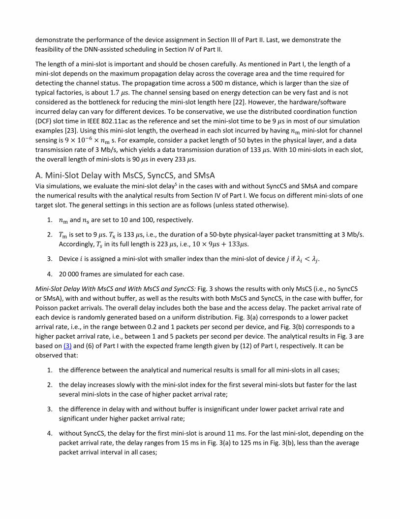
Mini-Slot Delay With MsCS and With MsCS and SyncCS: Fig. 3 shows the results with only MsCS (i.e., no SyncCS or SMsA), with and without buffer, as well as the results with both MsCS and SyncCS, in the case with buffer, for Poisson packet arrivals. The overall delay includes both the base and the access delay. The packet arrival rate of each device is randomly generated based on a uniform distribution. Fig. 3(a) corresponds to a lower packet arrival rate, i.e., in the range between 0.2 and 1 packets per second per device, and Fig. 3(b) corresponds to a higher packet arrival rate, i.e., between 1 and 5 packets per second per device. The analytical results in Fig. 3 are based on (3) and (6) of Part I with the expected frame length given by (12) of Part I, respectively. It can be observed that:

1. the difference between the analytical and numerical results is small for all mini-slots in all cases;

2. the delay increases slowly with the mini-slot index for the first several mini-slots but faster for the last several mini-slots in the case of higher packet arrival rate;

3. the difference in delay with and without buffer is insignificant under lower packet arrival rate and significant under higher packet arrival rate;

4. without SyncCS, the delay for the first mini-slot is around 11 ms. For the last mini-slot, depending on the packet arrival rate, the delay ranges from 15 ms in Fig. 3(a) to 125 ms in Fig. 3(b), less than the average packet arrival interval in all cases;

5. with SyncCS, the delay is reduced by more than 50% for each mini-slot as compared with the case without SyncCS. In the case of a higher packet arrival rate in Fig. 3(b), the maximum delay decreases from about 125 ms to around 35 ms.

Overall, the numerical results demonstrate the accuracy of (3) and (6) of Part I, the practicality of accommodating multiple devices in the same slot via MsCS, as well as the effectiveness of SyncCS.

Fig. 3. Mini-slot delay of MsCS only and of MsCS and SyncCS with (a) lower packet arrival rates and (b) higher packet arrival rates.

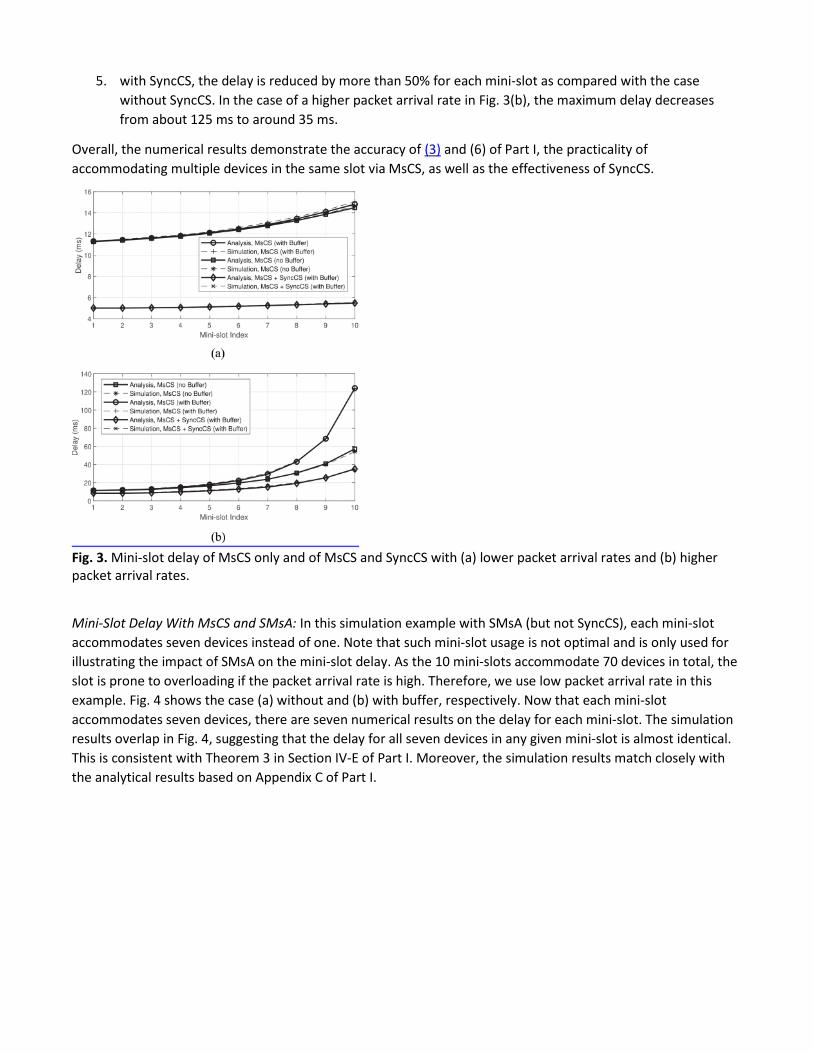
Mini-Slot Delay With MsCS and SMsA: In this simulation example with SMsA (but not SyncCS), each mini-slot accommodates seven devices instead of one. Note that such mini-slot usage is not optimal and is only used for illustrating the impact of SMsA on the mini-slot delay. As the 10 mini-slots accommodate 70 devices in total, the slot is prone to overloading if the packet arrival rate is high. Therefore, we use low packet arrival rate in this example. Fig. 4 shows the case (a) without and (b) with buffer, respectively. Now that each mini-slot accommodates seven devices, there are seven numerical results on the delay for each mini-slot. The simulation results overlap in Fig. 4, suggesting that the delay for all seven devices in any given mini-slot is almost identical. This is consistent with Theorem 3 in Section IV-E of Part I. Moreover, the simulation results match closely with the analytical results based on Appendix C of Part I.

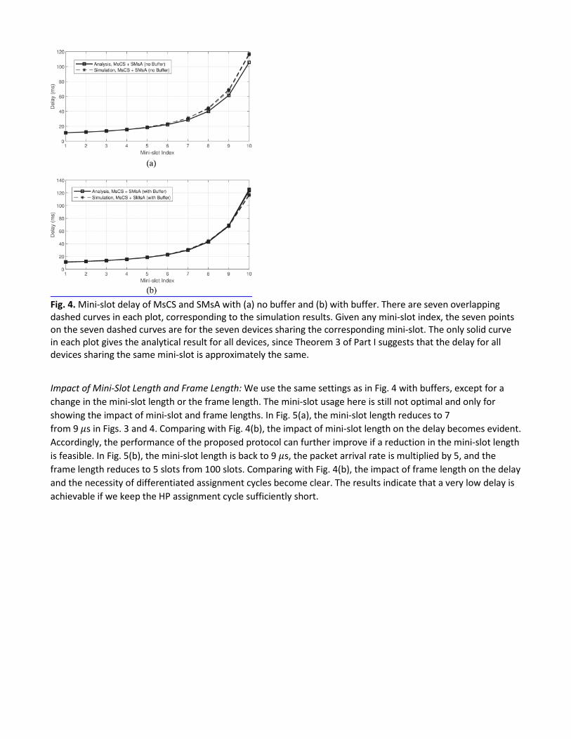
Fig. 4. Mini-slot delay of MsCS and SMsA with (a) no buffer and (b) with buffer. There are seven overlapping dashed curves in each plot, corresponding to the simulation results. Given any mini-slot index, the seven points on the seven dashed curves are for the seven devices sharing the corresponding mini-slot. The only solid curve in each plot gives the analytical result for all devices, since Theorem 3 of Part I suggests that the delay for all devices sharing the same mini-slot is approximately the same.

Impact of Mini-Slot Length and Frame Length: We use the same settings as in Fig. 4 with buffers, except for a change in the mini-slot length or the frame length. The mini-slot usage here is still not optimal and only for showing the impact of mini-slot and frame lengths. In Fig. 5(a), the mini-slot length reduces to 7 from 9 𝜇𝜇s in Figs. 3 and 4. Comparing with Fig. 4(b), the impact of mini-slot length on the delay becomes evident. Accordingly, the performance of the proposed protocol can further improve if a reduction in the mini-slot length is feasible. In Fig. 5(b), the mini-slot length is back to 9 𝜇𝜇s, the packet arrival rate is multiplied by 5, and the frame length reduces to 5 slots from 100 slots. Comparing with Fig. 4(b), the impact of frame length on the delay and the necessity of differentiated assignment cycles become clear. The results indicate that a very low delay is achievable if we keep the HP assignment cycle sufficiently short.

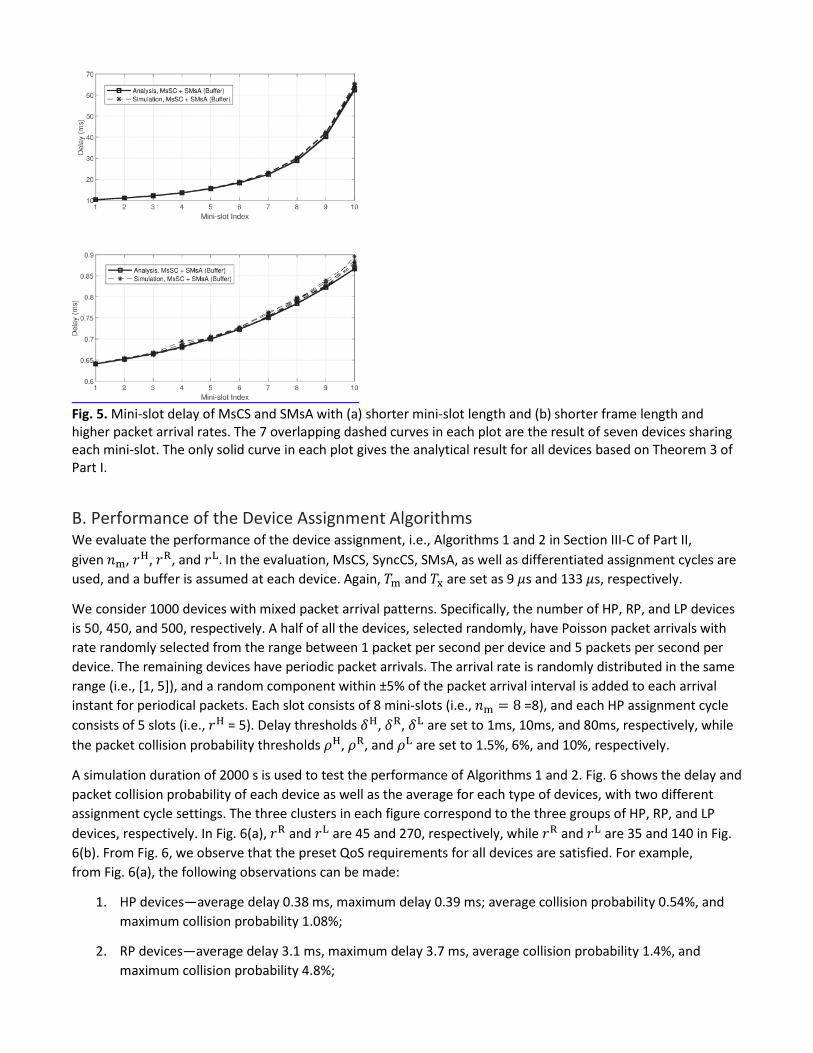
Fig. 5. Mini-slot delay of MsCS and SMsA with (a) shorter mini-slot length and (b) shorter frame length and higher packet arrival rates. The 7 overlapping dashed curves in each plot are the result of seven devices sharing each mini-slot. The only solid curve in each plot gives the analytical result for all devices based on Theorem 3 of Part I.

B. Performance of the Device Assignment Algorithms We evaluate the performance of the device assignment, i.e., Algorithms 1 and 2 in Section III-C of Part II, given 𝑛𝑛m, 𝑟𝑟H, 𝑟𝑟R, and 𝑟𝑟L. In the evaluation, MsCS, SyncCS, SMsA, as well as differentiated assignment cycles are used, and a buffer is assumed at each device. Again, 𝑇𝑇m and 𝑇𝑇x are set as 9 𝜇𝜇s and 133 𝜇𝜇s, respectively.

We consider 1000 devices with mixed packet arrival patterns. Specifically, the number of HP, RP, and LP devices is 50, 450, and 500, respectively. A half of all the devices, selected randomly, have Poisson packet arrivals with rate randomly selected from the range between 1 packet per second per device and 5 packets per second per device. The remaining devices have periodic packet arrivals. The arrival rate is randomly distributed in the same range (i.e., [1, 5]), and a random component within ±5% of the packet arrival interval is added to each arrival instant for periodical packets. Each slot consists of 8 mini-slots (i.e., 𝑛𝑛m = 8 =8), and each HP assignment cycle consists of 5 slots (i.e., 𝑟𝑟H = 5). Delay thresholds 𝛿𝛿H, 𝛿𝛿R, 𝛿𝛿L are set to 1ms, 10ms, and 80ms, respectively, while the packet collision probability thresholds 𝜌𝜌H, 𝜌𝜌R, and 𝜌𝜌L are set to 1.5%, 6%, and 10%, respectively.

A simulation duration of 2000 s is used to test the performance of Algorithms 1 and 2. Fig. 6 shows the delay and packet collision probability of each device as well as the average for each type of devices, with two different assignment cycle settings. The three clusters in each figure correspond to the three groups of HP, RP, and LP devices, respectively. In Fig. 6(a), 𝑟𝑟R and 𝑟𝑟L are 45 and 270, respectively, while 𝑟𝑟R and 𝑟𝑟L are 35 and 140 in Fig. 6(b). From Fig. 6, we observe that the preset QoS requirements for all devices are satisfied. For example, from Fig. 6(a), the following observations can be made:

1. HP devices—average delay 0.38 ms, maximum delay 0.39 ms; average collision probability 0.54%, and maximum collision probability 1.08%;

2. RP devices—average delay 3.1 ms, maximum delay 3.7 ms, average collision probability 1.4%, and maximum collision probability 4.8%;

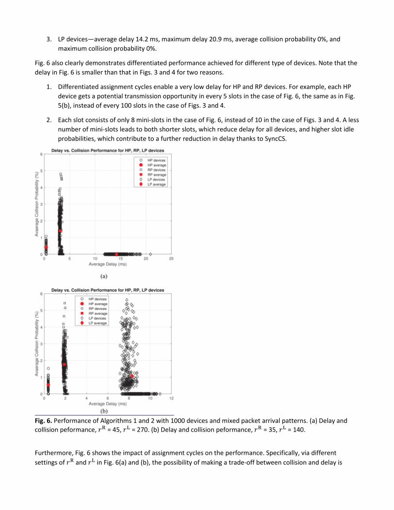
3. LP devices—average delay 14.2 ms, maximum delay 20.9 ms, average collision probability 0%, and maximum collision probability 0%.

Fig. 6 also clearly demonstrates differentiated performance achieved for different type of devices. Note that the delay in Fig. 6 is smaller than that in Figs. 3 and 4 for two reasons.

1. Differentiated assignment cycles enable a very low delay for HP and RP devices. For example, each HP device gets a potential transmission opportunity in every 5 slots in the case of Fig. 6, the same as in Fig. 5(b), instead of every 100 slots in the case of Figs. 3 and 4.

2. Each slot consists of only 8 mini-slots in the case of Fig. 6, instead of 10 in the case of Figs. 3 and 4. A less number of mini-slots leads to both shorter slots, which reduce delay for all devices, and higher slot idle probabilities, which contribute to a further reduction in delay thanks to SyncCS.

Fig. 6. Performance of Algorithms 1 and 2 with 1000 devices and mixed packet arrival patterns. (a) Delay and collision peformance, 𝑟𝑟R = 45, 𝑟𝑟L = 270. (b) Delay and collision peformance, 𝑟𝑟R = 35, 𝑟𝑟L = 140.

Furthermore, Fig. 6 shows the impact of assignment cycles on the performance. Specifically, via different settings of 𝑟𝑟R and 𝑟𝑟L in Fig. 6(a) and (b), the possibility of making a trade-off between collision and delay is

shown. Moreover, Fig. 6(a) and (b) demonstrates how our proposed algorithms can adapt to the given protocol parameters. In Fig. 6(a), 𝑟𝑟L is larger and each LP device has to wait for a longer duration before having a transmission opportunity. As a result, the probability that an LP device has a packet to send in its assigned mini-slot can be high, and assigning two or more LP devices the same mini-slot in such case can yield a high collision probability. Therefore, the algorithms choose to assign each LP device an exclusive mini-slot. In comparison, 𝑟𝑟L is much smaller in Fig. 6(b), and thus the probability that an LP device has a packet to send in its assigned mini-slot is lower. Therefore, the algorithms allow LP devices to share a mini-slot at the cost of small collision probabilities.

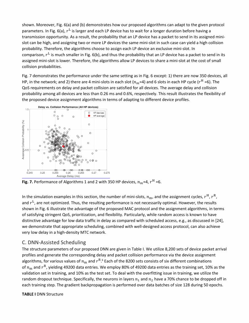
Fig. 7 demonstrates the performance under the same setting as in Fig. 6 except: 1) there are now 350 devices, all HP, in the network; and 2) there are 4 mini-slots in each slot (𝑛𝑛𝑚𝑚=4) and 6 slots in each HP cycle (𝑟𝑟H =6). The QoS requirements on delay and packet collision are satisfied for all devices. The average delay and collision probability among all devices are less than 0.26 ms and 0.6%, respectively. This result illustrates the flexibility of the proposed device assignment algorithms in terms of adapting to different device profiles.

Fig. 7. Performance of Algorithms 1 and 2 with 350 HP devices, 𝑛𝑛𝑚𝑚=4, 𝑟𝑟H =6.

In the simulation examples in this section, the number of mini-slots, 𝑛𝑛m, and the assignment cycles, 𝑟𝑟H, 𝑟𝑟R, and 𝑟𝑟L, are not optimized. Thus, the resulting performance is not necessarily optimal. However, the results shown in Fig. 6 illustrate the advantage of the proposed MAC protocol and the assignment algorithms, in terms of satisfying stringent QoS, prioritization, and flexibility. Particularly, while random access is known to have distinctive advantage for low data traffic in delay as compared with scheduled access, e.g., as discussed in [24], we demonstrate that appropriate scheduling, combined with well-designed access protocol, can also achieve very low delay in a high-density MTC network.

C. DNN-Assisted Scheduling The structure parameters of our proposed DNN are given in Table I. We utilize 8,200 sets of device packet arrival profiles and generate the corresponding delay and packet collision performance via the device assignment algorithms, for various values of 𝑛𝑛m and 𝑟𝑟R.6 Each of the 8200 sets consists of six different combinations of 𝑛𝑛m and 𝑟𝑟R, yielding 49200 data entries. We employ 80% of 49200 data entries as the training set, 10% as the validation set in training, and 10% as the test set. To deal with the overfitting issue in training, we utilize the random dropout technique. Specifically, the neurons in layers 𝑛𝑛1 and 𝑛𝑛2 have a 70% chance to be dropped off in each training step. The gradient backpropagation is performed over data batches of size 128 during 50 epochs.

TABLE I DNN Structure

Layer Number of neurons Activation function Dropout 𝑛𝑛1 1024 elu 70% 𝑛𝑛2 1024 elu 70% 𝑛𝑛3 512 elu - 𝑛𝑛4 256 relu - 𝑛𝑛5 128 relu - 𝑛𝑛6 64 relu - 𝑛𝑛7 13 relu -

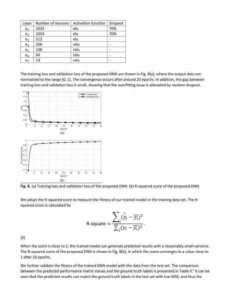
The training loss and validation loss of the proposed DNN are shown in Fig. 8(a), where the output data are normalized to the range [0, 1]. The convergence occurs after around 20 epochs. In addition, the gap between training loss and validation loss is small, showing that the overfitting issue is alleviated by random dropout.

Fig. 8. (a) Training loss and validation loss of the proposed DNN. (b) R-squared score of the proposed DNN.

We adopt the R-squared score to measure the fitness of our trained model in the training data set. The R-squared score is calculated by

R-square =� (𝑦𝑦

^𝑖𝑖 − 𝑦𝑦𝑖𝑖)2

𝑖𝑖� (𝑦𝑦𝑖𝑖 − 𝑦𝑦𝑖𝑖)2𝑖𝑖

.

(5)

When the score is close to 1, the trained model can generate predicted results with a reasonably small variance. The R-squared score of the proposed DNN is shown in Fig. 8(b), in which the score converges to a value close to 1 after 10 epochs.

We further validate the fitness of the trained DNN model with the data from the test set. The comparison between the predicted performance metric values and the ground truth labels is presented in Table II.7 It can be seen that the predicted results can match the ground truth labels in the test set with low MSE, and thus the

proposed DNN is able to learn the mapping from the device and packet arrival profile and the protocol parameter settings to the resulting performance after sufficient training.

TABLE II Comparison Between Predicted Results and Labels in the Test Set

Overall MSE Collision Probability Maximum MSE Mean MSE HP LP RP HP LP RP 2.3e-4 2.9e-5 - 1.8e-4 1.2e-6 - 1.6 e-5 Flag Bit Accuracy Delay Maximum MSE Mean MSE HP LP RP HP LP RP 98.5% 5.8e-9 I 4.0e-5 2.6e-7 5.0e-9 1.4e-5 1.5e-7

SECTION VI. Conclusion In Part II of this article, we customize scheduling for our proposed MAC protocol in Part I to complete the overall MAC protocol design. To maximize the strength of the MAC protocol, a proper choice of the cycle lengths and number of mini-slots in each slot is necessary, and so is a proper assignment of slots and mini-slots to all devices. Based on the performance analysis in Part I, we are able to assign devices with the due granularity and accuracy. Utilizing a trained DNN, we manage to determine the protocol parameters efficiently. Integrating the distributed coordination in Part I and the centralized scheduling in Part II composes the unique strength of our tailored MAC design. As a result, the proposed MAC is capable of supporting a large number of devices with sporadic data packets under a single AP and a single channel, while achieving a (sub)millisecond-level delay and very low collision probability. Building on the proposed MAC, future research directions may include extending the MAC design to nonfully connected networks with either one AP or multiple APs. Another possible extension is additional transmission control measures, such as random back-off or probabilistic transmission for improved fairness or further reduced collision probability.

ACKNOWLEDGMENT The authors would like to thank Conghao Zhou and Xuehan Ye for discussions on the role of learning in scheduling.

References 1. Y. Liu, M. Kashef, K. B. Lee, L. Benmohamed and R. Candell, "Wireless network design for emerging IIoT

applications: Reference framework and use cases", Proc. IEEE, vol. 107, no. 6, pp. 1166-1192, Jun. 2019. 2. J. Gao, W. Zhuang, M. Li, X. Shen and X. Li, "MAC for machine-type communications in industrial IoT—Part I:

Protocol design and analysis", IEEE Internet Things J., Jan. 2021. 3. D. Jiang, H. Wang, E. Malkamaki and E. Tuomaala, "Principle and Performance of Semi-persistent Scheduling

for VoIP in LTE System", Proc. Int. Conf. Wireless Commun. Netw. Mobile Comput. (WiCOM), pp. 2861-2864, Sep. 2007.

4. P. Wang and W. Zhuang, "A token-based scheduling scheme for WLANs supporting voice/data traffic and its performance analysis", IEEE Trans. Wireless Commun., vol. 7, no. 5, pp. 1708-1718, May 2008.

5. A. T. Gamage, H. Liang and X. Shen, "Two time-scale cross-layer scheduling for cellular/WLAN interworking", IEEE Trans. Commun., vol. 62, no. 8, pp. 2773-2789, Aug. 2014.

6. A. Ksentini, P. A. Frangoudis, P. C. Amogh and N. Nikaein, "Providing low latency guarantees for slicing-ready 5G systems via two-level MAC scheduling", IEEE Netw., vol. 32, no. 6, pp. 116-123, Nov./Dec. 2018.

7. A. S. Lioumpas and A. Alexiou, "Uplink scheduling for machine-to-machine communications in LTE-based cellular systems", Proc. GLOBECOM Workshops, pp. 353-357, Dec. 2011.

8. T. A. Al-Janabi and H. S. Al-Raweshidy, "An energy efficient hybrid MAC protocol with dynamic sleep-based scheduling for high density IoT networks", IEEE Internet Things J., vol. 6, no. 2, pp. 2273-2287, Apr. 2019.

9. P. Si, J. Yang, S. Chen and H. Xi, "Adaptive massive access management for QoS guarantees in M2M communications", IEEE Trans. Veh. Technol., vol. 64, no. 7, pp. 3152-3166, Jul. 2015.

10. G. Karadag, R. Gul, Y. Sadi and S. C. Ergen, "QoS-constrained semi-persistent scheduling of machine-type communications in cellular networks", IEEE Trans. Wireless Commun., vol. 18, no. 5, pp. 2737-2750, May 2019.

11. C. Zhang, X. Sun, J. Zhang, X. Wang, S. Jin and H. Zhu, "Throughput optimization with delay guarantee for massive random access of M2M communications in industrial IoT", IEEE Internet Things J., vol. 6, no. 6, pp. 10077-10092, Dec. 2019.

12. O. Arouk, A. Ksentini and T. Taleb, "Group paging-based energy saving for massive MTC accesses in LTE and beyond networks", IEEE J. Sel. Areas Commun., vol. 34, no. 5, pp. 1086-1102, May 2016.

13. N. Salodkar, A. Karandikar and V. S. Borkar, "A stable online algorithm for energy-efficient multiuser scheduling", IEEE Trans. Mobile Comput., vol. 9, no. 10, pp. 1391-1406, Oct. 2010.

14. C. Chang, D. Lee and C. Wang, "Asynchronous grant-free uplink transmissions in multichannel wireless networks with heterogeneous QoS guarantees", IEEE/ACM Trans. Netw., vol. 27, no. 4, pp. 1584-1597, Aug. 2019.

15. V. Rodoplu, M. Nakıp, D. T. Eliiyi and C. Güzeliş, "A multi-scale algorithm for joint forecasting-scheduling to solve the massive access problem of IoT", IEEE Internet Things J., vol. 7, no. 8, pp. 8572-8589, Sep. 2020.

16. B. Yang, X. Cao, Z. Han and L. Qian, "A machine learning enabled MAC framework for heterogeneous Internet-of-Things networks", IEEE Trans. Wireless Commun., vol. 18, no. 7, pp. 3697-3712, Jul. 2019.

17. B. Yang, X. Cao, J. Bassey, X. Li and L. Qian, "Computation offloading in multi-access edge computing: A multi-task learning approach", IEEE Trans. Mobile Comput., Apr. 2020.

18. A. Kumcu, K. Bombeke, L. Platiša, L. Jovanov, J. Van Looy and W. Philips, "Performance of four subjective video quality assessment protocols and impact of different rating preprocessing and analysis methods", IEEE J. Sel. Topics Signal Process., vol. 11, no. 1, pp. 48-63, Feb. 2017.

19. F. Chollet, Keras: The Python Deep Learning Library, Jun. 2018, [online] Available: https://ui.adsabs.harvard.edu/abs/2018ascl.soft06022C.

20. D. P. Kingma and J. Ba, Adam: A method for stochastic optimization, 2014, [online] Available: https://arXiv:1412.6980.

21. N. Srivastava, G. Hinton, A. Krizhevsky, I. Sutskever and R. Salakhutdinov, "Dropout: A simple way to prevent neural networks from overfitting", J. Mach. Learn. Res., vol. 15, no. 1, pp. 1929-1958, Jan. 2014.

22. S. Yoon, L. E. Li, S. C. Liew, R. R. Choudhury, I. Rhee and K. Tan, "QuickSense: Fast and energy-efficient channel sensing for dynamic spectrum access networks", Proc. IEEE INFOCOM, pp. 2247-2255, Apr. 2013.

23. IEEE, 802.11-2016, "IEEE Standard for Information Technology—Telecommunications and Information Exchange Between Systems Local and Metropolitan Area Networks—Specific Requirements—Part 11: Wireless LAN Medium Access Control (MAC) and Physical Layer (PHY) Specifications", Dec. 2016.

24. M. Gharbieh, H. ElSawy, H.-C. Yang, A. Bader and M.-S. Alouini, "Spatiotemporal model for uplink IoT traffic: Scheduling and random access paradox", IEEE Trans. Wireless Commun., vol. 17, no. 12, pp. 8357-8372, Dec. 2018.

Footnotes 1. The upper bound is obtained under the assumption that every HP device is assigned the first mini-slot of a

slot.

2. In practice, a guard margin may need to be applied to the estimated collision probability in (4a) . After all, such estimation may not be sufficiently accurate since we assume no statistical knowledge of the packet arrival of any device other than the average arrival rate.

3. Such complexity, as the result of a mixed integer nonlinear programming, is noted in many works, e.g., [17] , some of which adopt a learning-based method as a solution.

4. We refer to the collective information including the number of HP, RP, and LP devices as well as the packet arrival rate of each device as a device and packet arrival rate profile.

5. For brevity, we use “mini-slot delay” to refer to the delay of a device assigned that mini-slot. 6. We fix 𝑟𝑟H and 𝑟𝑟L in this illustration for simplicity. 7. The LP devices always have 0 collision probability in this example [similar to the case in Fig. 6(a)Fig. 6(a) ].

Thus, the MSE is 0 but not meaningful in such cases. Therefore, we use two “–” under LP instead of “0” in this table.