Mach’s principle and the dynamics of galaxies: v2 Nov 2012msp.warwick.ac.uk/~cpr/paradigm/galactic-dynamics-v2.pdf · 2013-01-17 · Mach’s principle and the dynamics of galaxies:

Mach’s principle and the dynamics of galaxies: v2 Nov 2012

COLIN ROURKE

A basic model for the dynamics of galaxies is given which explains the anomalousrotation curves and the predominant spiral structure without the need for “darkmatter”. The model is based on a metric inspired by Mach’s principle but whichmay not satisfy Einstein’s equations.

85A05; 85A15, 85A40, 83F05, 83C40, 83C57

1 Introduction

This paper is part of a joint project with Robert MacKay to understand cosmology ingeneral, and the dynamics of galaxies in particular, using a fully relativistic approach,without recourse to “dark matter” or other unobserved hypotheses. This paper adoptsan interim approach. It uses a metric which is obtained by perturbing a standard metricto make it model a specific formulation of Mach’s principle. The perturbation stops themetric from satisfying Einstein’s equations and therefore the approach adopted here isnot fully relativistic. We hope in the future to find a metric which does satisfy Einstein’sequations and which gives a similar dynamic. This paper can be seen as motivation forthe search for this metric.

Mach’s principle [21] is the principle that the local concept of inertial frame is correlatedwith the distribution of the matter in the universe. The principle is often stated usingthe wording “determined by” rather than “correlated with”. However this formulationbegs the question of how this determination takes place and we prefer a less contentiousstatement.

It is well known that solutions to Einstein’s equations need not satisfy Mach’s principle,see eg Rindler [27]. One particular solution which breaks Mach’s principle and which isgermane to the main subject matter of this paper is the Kerr solution for the metric neara rotating mass in an otherwise empty universe. In the Kerr universe there is only onecentral mass and no other mass to determine the inertia of the central mass. If the solutionwere Machian then the inertial frame at every other point would rotate with the centralmass and the solution would be a simple coordinate transformation of the Schwarzschild

http://www.ams.org/mathscinet/search/mscdoc.html?code=85A05,(85A15, 85A40, 83F05, 83C40, 83C57)

2 Colin Rourke

solution. In a similar way, the Lense–Thirring effect [33] (frame-dragging near arotating body) is also based on a distribution of matter with just one rotating object andno other mass to determine its rotation, and is therefore non-Machian. A more preciseway in which this effect breaks Mach’s principle is given in [27] and will be discussedfurther below.

We formulate Mach’s principle in a similar way to that given in Misner, Thorne andWheeler [22, pages 543–549]. In particular we assume that the rotation of the localinertial frame is given as the weighted sum of the rotations of all other inertial frames forall the matter in the universe as suggested in [22, equations 21.159–60]. Now supposethat there is a compact and locally isolated rotating mass at the origin. The conceptof inertial frame near the origin is correlated with the rotation of the central mass andframes will tend to rotate in the same sense. The “simple dimensional considerations”mentioned in [22, page 547, above equation 21.155] show that this frame draggingeffect (which from now on we refer to as inertial drag) is proportional to Mµ/r , whereM , µ are mass and angular velocity of the central mass and r is distance from theorigin. Lense–Thirring frame dragging is not Machian in this formulation because, nearthe equator, the frame is dragged in the opposite sense to the rotation of the centralmass [22, page 548, 21.157]. It is this point that Rindler (op cit) makes to “expose” theLense–Thirring effect as non-Machian1. Rindler’s conclusion is that Mach’s principleneeds to be treated with care “one simply cannot trust Mach!”. Our conclusion is theopposite. Mach’s principle is the only sane way to understand the origin of inertia in theuniverse and we must restrict to solutions of Einstein’s equations which are Machian.In particular the Kerr solution is not a valid model for the metric near a rotating massand we need to find a Machian rotation metric (an MR–metric) to replace it. The factthat it is possible to construct non-Machian solutions to Einstein’s equations does notimply that Mach’s principle is somehow incompatible with Einstein. The Kerr metric isbased on a particular set of boundary conditions (rotating central mass and flat, zeromass, at infinity). These boundary conditions are in themselves non-Machian and henceany solution which fits them must also break Mach’s principle. With good boundaryconditions there may well be Machian solutions and this is what we hope to find. Thismay not be an easy task. There are good reasons to expect a valid metric not to be staticfor example, and there is no reason to expect it to have nice properties at infinity. Indeedit may be the case that a property of rotating masses is that they generate gravitationalwaves of a spectrum of frequencies and therefore the metric may have no symmetries.

1See also the discussion Appendix A: the Lense–Thirring effect is based on a first orderperturbation of the flat metric and therfore is unlikely to apply to a metric with a heavy rotatingbody in it.

Mach’s principle and the dynamics of galaxies: v2 Nov 2012 3

See Appendix A for further discussion of Mach’s principle.

We hope to make progress on the problem of finding a satisfactory MR–metric in futurejoint papers. This paper is intended to motivate this search and to give some of theproperties of the desired metric. In particular it is shown here that a suitable MR–metricwill solve one of the major outstanding problems of cosmology, namely the nature ofthe spiral arms in a normal galaxy, for which there is no present satisfactory explanation.Using the interim metric studied here, a model for the dynamics of spiral galaxies isgiven which fits observations and has no need for exotic hypotheses (eg a fortuitousdistribution of unobserved dark matter). The basic idea is that the centre of a normalspiral galaxy such as the Milky Way contains a hypermassive black hole, of mass 1011

solar masses or more, as has been observed for active galaxies, and that this blackhole emits jets of light particles, which condense into stellar systems as they progressoutwards2. The visible arm structure is formed by the condensing particle streams andthe resulting star creation regions, which move outwards along the arms as they rotatearound the centre. The dynamic is directly controlled by the massive centre and theprincipal engine for the dynamic is inertial drag. The model we obtain has fairly simplesolution curves and we use Mathematica to sketch them and to sketch the resultingappearance of the galaxy.

The interim metric is obtained by perturbing a standard spherically-symmetric metricby adding a variable rotation about the z–axis. This builds in a specific inertial drageffect and we choose this to fit the formulation of Mach’s principle given above. It isquite different from the Kerr metric and in particular it is not static. We believe thatinertial drag is the major relativistic effect in this context and therefore that the modelthat we construct here is close to the accurate MR–metric model that we hope to find inthe future.

The fit with observations that we find is good but not perfect and we expect to betterit with the real metric. Also we ignore all non-symmetrical masses and with a morerealistic model, taking into account for example the mass of the arms themselves, weagain expect a better fit.

The paper is organised as follows. We start in Section 2 by formulating the interimmetric and using it to find an expression for the tangential velocity of a particle, moving

2There are two very unfortunate pieces of terminology here. All galaxies are active accordingto the model for spiral structure proposed in this paper and the distinction between active andnormal is just whether the central black hole is totally masked (as it is for a normal galaxy) ornot. Moreover it is well-known that black holes (especially supermassive ones) are anything butblack. However this second piece of terminology is well-established and we shall continue touse it.

4 Colin Rourke

in the plane of rotation of a heavy rotating body, in terms of r (distance from the centre).This models accurately the characteristic rotation curve for a galaxy. In Section 3 weadd radial motion and find an expression for radial velocity (again in terms of r). Theseexpressions allow us to use Mathematica to sketch both the orbits and the final shape ofthe galaxy, which is done in Section 4. Throughout the paper you should bear in mindthat we are modelling observed spiral galaxies and you should compare our sketcheswith real galaxies. To help you, we have reproduced five good examples, M83, M101,NGC1300, NGC1365 and M51, Figures 1, 2 and 3.

Figure 1: M83 Southern Pinwheel: image from European Southern Observatory

In Section 5 we put forward a tentative model for the central mechanism which generatesspiral arms. This suggests a natural reason why the asymptotic rotation velocity isconstant within a small factor across many different galaxies. In Section 6 we discussother observations and how they fit with the model proposed here. Topics considered


are: early 21cm observations, stellar populations, Sagittarius A∗ , the position of thesun, globular clusters and local stellar velocities (with details deferred to AppendixB). In Section 7 we speculate on wider cosmological issues and finally there are twoappendices, A on Mach’s principle and B on local stellar velocities.

Figure 2: M101 (left) and NGC1300 (right): images from the Hubble site [4]

2 The rotation curve

Observed rotation curves for galaxies are quite striking. Typically the curve (of tangentialvelocity against distance from the centre) comprises two approximately straight lineswith a short transition region. The first line passes through the origin, in other wordsrotation near the centre has constant angular velocity (plate-like rotation); the secondis horizontal, in other words the tangential velocity is asymptotically constant, seeFigure 5 (right) below. Furthermore, observations show that the horizontal straight linesection of the rotation curve extends far outside the limits of the main visible parts ofgalaxies and the actual velocity is constant within less than an order of magnitude overall galaxies observed (typically between 100 and 300km/s).

In this section we model rotation curves by using the interim metric.

Precise formulation of inertial drag

We start by formulating precisely the inertial drag effect mentioned in the introduction.

Consider a rotating body of mass M at the origin rotating in the right-hand sense aboutthe z–axis with angular velocity µ. In the main application that we have in mind, thismass will be the central black hole in a galaxy of somewhere between 1011 and 1013

6 Colin Rourke

solar masses but the analysis applies to any rotating body. As explained above, as aconsequence of Mach’s principle the body causes the local inertial frame to rotate inthe same sense. The local inertial frame rotates with respect to distant galaxies by theweighted sum of µ weighted kM/r and 0 (for all the distant “stationary” galaxies)weighted Q say where r is distance from the origin. We can normalise the weighting sothat Q = 1 (which is the same as replacing k/Q by k) which leaves just one constant kto be determined by experiment or theory. The nett effect is a rotation of

(1)(kM/r)× µ+ 1× 0

(kM/r) + 1=

Ar + K

where K = kM and A = Kµ.

Side note There is some evidence that k is in fact 1 so that K = M . This follows fromthe observation made in [22, below 21.160] that the sum

∑mα/rα over all masses

mα in the universe (at distance rα ) is approximately 1, which makes the choice ofnormalised weighting, Q = 1, the same as weighting purely by mass3. This suggests adeep property of space-time, namely that a third concept of “mass” (the inertial dragmass) is the same as the other two (gravitational mass and ordinary inertial mass).However this speculation is not relevant to the arguments presented in this main part ofthe paper and will be relegated to Appendix A. Nothing that we prove here depends onknowing the exact relationship between K and M .

Figure 3: NGC1365 and M51 images from NASA and Hubble site resp

3By “universe” we mean the visible universe or more precisely our backward light cone.Then there are about 1011 galaxies of weight about 0.03 (1011 solar masses) at distances varyingup to 1010 , where we use natural units (G = c = 1 and everything is in measured in years).


The interim metric

We define the interim metric by adding a variable rotation factor to a spherically-symmetric metric.

The most general spherically-symmetric metric can be written in the form:

(2) ds2 = −Q dt2 + P dr2 + r2 dΩ2

where P and Q are positive functions of r and t on a suitable domain. Here t is time, ris “distance from the centre” (but see the note below) and dΩ2 , the standard metric onthe unit 2–sphere S2 , is an abbreviation for dθ2 + sin2 θ dφ2 . We orient the 2–sphereso that the z–axis passes through it at the north pole where θ = π/2. The (x, y)–plane(pasing through the origin and perpendicular to the z–axis) is the equatorial plane. TheSchwarzschild–de Sitter metric is the case

Q =1P

= 1− Λr2

3− 2M

rwith Λ and M constants. By Birkhoff’s theorem this is the only case where the metricsatisfies Einstein’s vacuum equations with cosmological constant in some region. Inthis case the metric is necessarily static in this region; for an elementary proof goingback to Christoffel symbols and proving rather more than is usally stated, see [30]. Notethat the special cases M = Λ = 0 and Λ = 0 give the Minkowski and Schwarzschildmetrics respectively.

Note It is important to observe that r is a coordinate which is not precisely the sameas distance in the metric. It is chosen so that the sphere of symmetry at coordinate rhas the geometry of a Euclidean sphere of radius r . Distance measured in the metricalong a radius near this sphere is not the same as change in the coordinate r (this onlyhappens if P takes the value 1 near the point under consideration).

We form the interim metric by adding a variable rotation about the z–axis. We do thisby replacing φ by φ− ωt . The metric is no longer diagonal:

(3) ds2 = (−Q+τ 2) dt2 + (P+σ2) dr2 +r2 dΩ2 +2στ dr dt−2ρσ dφ dr−2ρτ dφ dt

where ρ = r sin(θ), σ = ρω′t, τ = ρ(ω + ωt), and prime means differentiation wrt rand dot wrt t .

If ω is constant this is the same metric viewed through rotating glasses, but the wholepoint is to allow ω to vary. If we start with the Schwarzschild–de Sitter metric and makethis substitution with variable ω , the metric no longer satisfies Einstein’s equations. Itis not hard to see that the inertial frame at a point rotates about a line parallel to the

8 Colin Rourke

z–axis with angular velocity the value of ω at that point. This is clear if ω is constantand in general, provided ω is continuous, it follows from the locality of inertial frames.So to fit with inertial drag as formulated in (1) we need to set ω = A/(r + K) (at least inthe (x, y)–plane). However it is easy to work with a general function ω and specialisewhen we need to. We shall investigate the orbits of particles moving on geodesics in theequatorial plane and we shall find that, provided ω decreases like A/r as r →∞, theorbits fit observed rotation curves.

The interim metric (3) is axially-symmetric with axis the z–axis (θ = π/2) and it isoften convenient to use alternative coordinates (r, φ, z) where r is now restricted tothe equatorial plane (perpendicular to the z–axis or equivalently where θ = 0). Weshall assume that ω is independent of φ (in order to preserve axial-symmetry) and forsimplicity we also assume that it is independent of t . Thus we assume ω is a functionof (r, θ) or equivalently (r, z).

Note that even if P and Q are also independent of t the new metric will not be static(with dt giving a Killing vector field) because of the (ρω′t)2 dr2 term. For the metricto be static, we would need ω′ = 0, in other words ω constant, and the metric wouldnot be interesting. It is important that the metric not be static because it is well knownthat a local (ie extending to be asymptotically flat at infinity) axially-symmetric, staticmetric which satisfies Einstein’s equations is equivalent to the Kerr metric, which givesthe wrong drop-off for inertial drag to fit observed rotation curves.

Finding the rotation curve

We shall concentrate on geodesics lying in the equatorial plane and on the tangentialcomponent of the velocity. Let a particle move along a geodesic with total velocity wwith tangential component v (perpendicular to the line through the origin).

There are two effects which determine the relationship between v and r , ie the rotationcurve.

Effect 1 The slingshot effect

A particle which is stationary in the inertial frame at a particular value of r is in factmoving with tangential velocity ωr in our coordinates and hence has tangential velocityincreasing with r . Intuitively we expect this effect to increase v by the rule dv/dr = ω

and we shall make a precise statement and proof below. Now suppose that the inertialdrag effect is local ie that ω → 0 as r → ∞. Then this effect decreases to zero at∞ and the virtual tangential rotation due to rotation of the inertial frame becomes a


genuine tangential velocity. This is analogous to the familiar effect of releasing anobject swinging on a string and this is why we have called it “the slingshot effect.”

Effect 2 Conservation of angular momemtum

Roughly speaking this says that rv is constant and therefore this has the opposite effectof decreasing v with r . Some care is needed because v here has to be interpreted astangential velocity in the local inertial frame. The precise statement is given in theproof below.

We shall calculate the two effects together and we start by giving a proof of conservationof angular momemtum which applies to the interim metric.

Proof of conservation of angular momentum

Conservation of angular momemtum is a property of any system with a central force (orspace-time geometry which simulates a central force). It is not restricted to Newtonianphysics. We shall prove this by modifying Newton’s proof of the equal area law forplanetary orbits (which law is exactly the same as conservation of angular momemtum).The proof works in the interim metric (3) and we shall obtain a formula for both effectsat the same time. For the time being ignore ω (or set it equal to zero).

The idea is to replace the central force by a series of central impulses at equally spaced(small) intervals of time. Consider Figure 4, where prime no longer means differentiationwrt r . At a particular time the particle (of small unit mass) is at P and has just receiveda central impulse resulting in velocity w. Its tangential velocity at P is u = |AP|. Onesmall interval of time later the particle is at P′ and receives another central impulse(along the line OP′ ) which does not change its tangential velocity u′ = |P′B|. But thetriangle OPP′ can be regarded as having base r = |OP| and height u or base r′ = |OP′|and height u′ hence ur = u′r′ in other words the angular momentum at P is the sameas at P′ .

To obtain the result for an arbitrary continuous central force, we take the limit of asequence of central impulses. Note the proof does not use any property of the centralforce other than that it acts towards the centre. Nor does it assume that r represents agenuine distance in the metric under consideration. All that is needed is that Euclideangeometry correctly describes the relationship bewteen r and distances perpendicular toradii near Pand P′ which is precisely how r was chosen.

10 Colin Rourke

A

P′ B

P

O

u′

u

r′ r

ba w

Figure 4: Proof of conservation of angular momemtum

The fundamental relation

We now need to reinstate ω . We need to note that “force” in our model is a property oflocal space-time geometry. In the case that ω is constant, the inertial frame (rotatingwith ω ) is the same as the unrotated case and in this frame the force is central. Thereforeby locality it is central in the general case in the inertial frame. Therefore the proofjust given makes sense in the inertial frame at P′ in other words rotating with angularvelocity ω′ = ω(P′) though, as we shall see, in the limit we get the same result ifwe assume that we are in the frame rotating with angular velocity ω(P). To find therequired relationship bewteen v and r we write v for the full tangential velocity at Pand v′ at P′ . Since we are working in the frame rotating at ω′ we have v = u + ω′r ,v′ = u′ + ω′r′ . Write v′ = v + δv, u′ = u + δu, r′ = r + δr and ω′ = ω + δω .

From ur = u′r′ we find

(4) u δr + r δu = 0

to first order. But

δu = u′ − u = v′ − ω′r′ − (v− ω′r) = v′ − v− ω′(r′ − r) = δv− ω′ δr


and substituting for u, δu in (4) we find

(v− ω′r) δr + r(δv− ω′ δr) = 0

which givesr δv = 2rω′ δr − v.

We can replace ω′ by ω to first order (as forecast) and going to the limit we obtain thefundamental relation between v and r :

(5)dvdr

= 2ω − vr

We can understand (5) intuitively as follows. As remarked earlier, the slingshot effectintuitively produces an acceleration dv/dr = ω . On the other hand vinert = v− ωr isthe “inertial” tangential velocity (corrected for rotation of the local inertial frame) andtherefore conservation of angular momentum produces a deceleration in v of vinert/ror an acceleration dv/dr = ω − v/r . Adding the two effects gives the fundamentalrelation.

Solving to find rotation curves

Given ω as a function of r , (5) can be solved to give v as a function of r . We canrewrite it as

rdvdr

+ v = 2ωr .

The LHS is d/dr (rv) and we obtain the general solution

(6) v =1r

(∫2ωr dr + const

).

It is now clear that we can obtain any prescribed differentiable rotation curve by makinga suitable choice of continuous ω .

We are interested in solutions which, like observed rotation curves, are asymptoticallyconstant and inspecting (6) this happens precisely when

∫2ωr dr is asymptotically

equal to Cr for some C and this happens precisely when 2ω is asymptotically equal toC/r . We have now proved the following result.

Theorem The equatorial geodesics in the interim metric (3) have tangential velocityasymptotically equal to constant C if and only if ω is asymptotically equal to A/rwhere C = 2A.

12 Colin Rourke

The basic model

We now specialise to the case ω = A/(r + K) which gives the value of inertial dragformulated in (1).

From (6) we have:

v =1r

(∫2Ar

r + Kdr + C

)=

2Ar

(∫1− K

r + Kdr)

+Cr

= 2A− 2AKr

log( r

K+ 1)

+Cr

(7)

where C is a constant depending on initial conditions. For a particle ejected from thecentre with v = rω for r small, C = 0, and for general initial conditions there is acontribution C/r to v which does not affect the behaviour for large r . For the solutionwith C = 0 there are two asymptotes. For r small v ≈ rω and the curve is roughly astraight line through the origin. And for r large the curve approaches the horizontal linev = 2A. A rough graph is given in Figure 5 (left) where K = A = 1. The similaritywith a typical rotation curve, Figure 5 (right), is obvious. Note that no attempt has beenmade here to use meaningful units on the left. See Figure 7 below for curves from ourmodel using sensible units.

1

2

10 20 30 40

Figure 5: The rotation curve from the model (left) and for the galaxy NGC3198 (right) takenfrom Begeman [8]

There are other shapes for rotation curves and we refer to [32] for a survey. All agreeon the characteristic horizontal straight line. Figure 6 is reproduced from [32] and gives


a good selection of rotation curves superimposed. In Figure 7 we give a selection ofrotation curves again superimposed, sketched using Mathematica4 and the model givenhere. The different curves correspond to choices of A,K and C . The similarity is againobvious. The units used differ. In our model we always use natural units so that avelocity of .001 is 300km/s and a distance of 45,000 is 15Kpc approx.

Figure 6: A collection of rotation curves from [32]

10000 20000 30000 40000 50000

0.0005

0.0010

0.0015

Figure 7: A selection of rotation curves from the model

It is worth commenting that the observed rotation curve for a galaxy is not the sameas the rotation curve for one particle, which is what we have been modelling. Whenyou observe a galaxy, you see many particles at once and you expect to see a rotationcurve made from several close but not identical rotation curves for particles. Indeed,

4The notebook Rots.nb used to draw this figure can be collected from [5] and the values ofthe parameters used read off.

14 Colin Rourke

as we shall see in Section 5, galactic arms are generated by a series of explosions andare expected to be non-uniform. So we expect the observed rotation curves to havevariations from the modelled rotation curve for one particle, which is exactly what wesee in Figures 5 (right) and 6.

As remarked earlier, the effect described in this section is independent of mass. Howeverfor rotating bodies of small mass the effect is unobservably small. For example the sunhas K ≈ 3km and ω = 2π/25 days. Thus 2Kω is 6km per 4 days or .06 km per hour.

3 The full dynamic

We now extend the analysis of the last section to find a formula for the radial velocity(again in terms of r) and this will allow us to plot orbits.

Intuitively there are two radial “forces” on our particle: a centripetal force because ofthe attraction of the massive centre and a centrifugal force caused by rotation in excessof that due to inertial drag. Thus we expect a formula for radial acceleration

(8) r =v2

inert

r− F(r)

where vinert = v− ωr and F(r) is the effective central “force” at radius r , per unit mass.

We shall prove this in a similar way to the proof of conservation of angular momentumgiven in the last section, using a geometrical argument which is valid in the interimmetric.

Centrifugal force

The idea is the same as before, namely to replace the central force by a series of centralimpulses at equally spaced small intervals δt of time and then take the limit as δt→ 0.As in the previous proof, start by setting ω equal to zero. Consider Figure 4 once again.a = |AP′| is the outward velocity (ie r) at P (after the central impulse) and b = |PB| isthe outward velocity at P′ before the central impulse. The effect of the central impulseis to subtract F(r′) δt . Therefore if a′ denotes the value of r at P′ then a′ = b−F(r′) δtor

(9) a− b = −F(r′) δt − δa

where a′ = a + δa. But by Pythagoras a2 + u2 = ||w||2 = b2 + (u′)2 and hence

(a− b)(a + b) = δu (u + u′)


where δu = u′ − u as before. Then substituting for a− b from (9) we find

(10) (a + b)(−F(r′) δt − δa) = (u + u′) δu.

But recall that ur = u′r′ which implies

(11) u δr + r δu = 0

to first order where δr = r′ − r as before. Now multiply (10) by r , reverse sign andsubstitute for r δu from (11) to obtain:

(12) r (a + b)(δa + F(r′) δt) = u(u + u′) δr

But to first order a + b = 2δr/δt (recall that a is r), F(r′) = F(r) and u + u′ = 2u.Thus (12) simplifies to

δaδt

+ F(r) =u2

r.

In the limit δa/δt becomes da/dt = dr/dt = r and we have proved

(13) r =u2

r− F(r).

Now reinstate ω . Exactly as in the previous proof, by locality the proof just givenmakes sense in the inertial frame at P in other words rotating with angular velocityω = ω(P). But u = v− ωr = vinert and we have proved (8).

Computing radial velocity

We now specialise to the case ω = A/(r + K). In this case v is given by (7) and wehave:

(14) vinert = 2A− 2AKr

log( r

K+ 1)

+Cr− Ar

K + rMoreover for the purposes of investigation we shall assume that F(r) is the inversesquare law F(r) = M/r2 . This is correct for Minkowski space (see above for discussionof how central force works in the interim metric) and is a good approximation forSchwarzschild and Schwarzschild–de Sitter provided r is not small. Thus we have:

r =v2

inert

r− M

r2 =1r

[2A− 2AK

rlog( r

K+ 1)

+Cr− Ar

K + r

]2

− Mr2

Multiplying by r and integrating wrt t (using a computer integration package) we find

12 r2 =

∫rdr =− C2

2r2 +M − 2AC

r+

A2KK + r

+ A2 log(K + r)

+2AK(C + 2Ar) log(1 + r/K)− (2AK log(1 + r/K))2

r2 + E

16 Colin Rourke

where E is another constant depending on initial conditions. From this equation we canread off r (in terms of r). Moreover since we have a formula for v, we also have aformula for θ = v/r . Therefore we can express θ and t in terms of r as integrals. Theseintegrals are not easy to express in terms of elementary functions but Mathematica ishappy to integrate them numerically and we can use this to plot the orbits of particlesejected from the centre. If we now assume that the centre of a normal galaxy contains abelt structure similar to that hypothesised for “active” galaxies which emits streams ofparticles, then we can model the orbits and hence take a “snapshot” of all the orbits atan instant of time, in other words obtain a picture of the galaxy. We obtain excellentmodels for the observed spiral structure of normal spiral galaxies. We do this in thenext section. More detail on the proposed central generator for the spiral arms will begiven in Section 5.

Simplified equations

There is a very convenient simplification for the equations given in this section, whichhelps to explain how inertial drag controls the dynamic. For most of an orbit in a galaxyr K , since r varies up to 105 for the main visible disc whilst K ≈ M ≈ .1. Thismakes the fraction A/(K + r) close to A/r and the formulae for v and vinert reduce to2A + C/r and A + C/r respectively and we find

r =A2

r+

AC −Mr2 +

C2

r3 .

There are good reasons for setting C < 0 (see Section 5) so that the AC/r2 term acts toincrease the gravitational pull. But the positive terms A2/r and C2/r3 offset the centralgravitational pull (the first for large r and the second for small r) and this allows longslow outward orbits which fill out the spiral arms.

4 Mathematica generated pictures

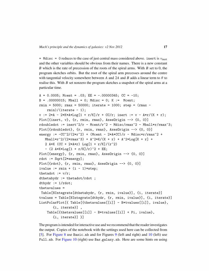
Below is the basic Mathematica notebook which generates galaxy pictures from thedynamics found in Section 3 above. The notation is as close as possible to the notationused before. A, K, r and v are A,K, r and v resp. E and C have been replaced by EE

and CC because E and C are reserved variables in Mathematica. M has been replaced bythree constants Mcent, Mdisc and Mball. This is to allow an investigation of the effectof significant non-central mass on the dynamic. Mcent acts exactly as M above whilstMdisc and Mball act as masses of a uniform disc or ball of radius rmax. Setting Mball


= Mdisc = 0 reduces to the case of just central mass considered above. inert is vinert

and the other variables should be obvious from their names. There is a new constantB which is the rate of precession of the roots of the spiral arms. With B set to 0, theprogram sketches orbits. But the root of the spiral arm precesses around the centrewith tangential velocity somewhere between A and 2A and B adds a linear term to θ torealise this. With B set nonzero the program sketches a snapshot of the spiral arms at aparticular time.

A = 0.0005; Mcent = .03; EE = -.00000345; CC = -10;

B = .00000015; Mball = 0; Mdisc = 0; K := Mcent;

rmin = 5000; rmax = 50000; iterate = 1000; step = (rmax -

rmin)/(iterate - 1);

v := 2*A - 2*K*A*Log[1 + r/K]/r + CC/r; inert := v - A*r/(K + r);

Plot[inert, v, r, rmin, rmax, AxesOrigin --> 0, 0]

rdoubledot := inert^2/r - Mcent/r^2 - Mdisc/rmax^2 - Mball*r/rmax^3;

Plot[rdoubledot, r, rmin, rmax, AxesOrigin --> 0, 0]

energy := -CC^2/(2*r^2) + (Mcent - 2*A*CC)/r - Mdisc*r/rmax^2 +

Mball*r^2/(2*rmax^3) + A^2*K/(K + r) + A^2*Log[K + r] +

2 A*K (CC + 2*A*r) Log[1 + r/K]/(r^2)

- (2 A*K*Log[1 + r/K]/r)^2 + EE;

Plot[energy, r, rmin, rmax, AxesOrigin --> 0, 0]

rdot := Sqrt[2*energy];

Plot[rdot, r, rmin, rmax, AxesOrigin --> 0, 0]

ivalue := rmin + (i - 1)*step;

thetadot := v/r;

dthetabydr := thetadot/rdot ;

dtbydr := 1/rdot;

thetavalues =

Table[NIntegrate[dthetabydr, r, rmin, ivalue], i, iterate]

tvalues = Table[NIntegrate[dtbydr, r, rmin, ivalue], i, iterate]

ListPolarPlot[ Table[thetavalues[[i]] - B*tvalues[[i]], ivalue,

i, iterate] ,

Table[thetavalues[[i]] - B*tvalues[[i]] + Pi, ivalue,

i, iterate] ]

The program is intended for interactive use and we recommend that the reader investigatesthe output. Copies of the notebook with the settings used here can be collected from[5]. For Figure 8 use Basic.nb and for Figures 9 (left and right) and 10 (left) useFull.nb. For Figure 10 (right) use Bar galaxy.nb. Here are some hints on using

18 Colin Rourke

it. As remarked earlier, the sketches are discrete plots obtained by repeated numericalintegration. The number of plot points is set by iterate. Start investigating withiterate = 100 which executes fairly quickly and then set iterate = 1000 for goodquality output. The plots are calculated in terms of r not time. You can read the timevalues from the tvalues table which is printed as part of the output. r varies in equalsteps from rmin to rmax which need to be preset. You can’t run to the natural limit forr (when r = 0) but have to stop before this happens.

-40000 -20000 20000 40000

-40000

-20000

20000

40000

Figure 8: Output from the program as printed

Set A to fit the desired asymptotic tangential velocity 2A. For example to get 2A ≈300km/s set A = 0.0005. Set Mcent to the desired central mass. For example 1011

and 1012 solar masses are M = .03 and .3 respectively. Leave K set to equal Mcentunless you want to experiment with large values (which will increase the inertial drageffect for a fixed mass). B needs to be set to somewhere near A/rmin. The integrationconstants C and E affect the picture mostly near the middle and outside resp. There aretheoretical reasons for setting C to be negative because of the nature of the spiral armgenerator (see Section 5) and with C set negative, the roots of the spiral arms are offsetin a way seen in many galaxy examples. E is a key setting as it determines the energyof orbits and hence the overall size of the galaxy. To get the most realistic pictures youneed r to go to almost to zero at the maximum for r which you get by fine tuning E .To help with this tuning, the program plots the graphs of v, vinert, r, energy and r sothat you can adjust to get r and r near zero at rmax.


We now give some plots of orbits and galaxy arms obtained from this program. Theseshould be compared with the images of real galaxies that we have reproduced (Figures1, 2 and 3).

Figure 8 is the output from the program as printed above. M has been set to 1011 solarmasses (all central) with tangential velocity asymptotic to 300km/s, and B has beenset to A/rmin and rmax to 50,000 light years (corresponding to a visible diameter of100,000 light years). Time elapsed along the visible arms is 5.5× 107 years. See thediscussion of the correct figure here in Section 6 below.

-40000 -20000 20000 40000

-15000

-10000

-5000

5000

10000

15000

-40000 -20000 20000 40000

-40000

-20000

20000

40000

Figure 9: Left: orbits. Right: loose spiral

In Figures 9 (left and right) and 10 (left) we have the same settings with only B varied.The settings are similar to Figure 8 but with a small realistic contribution to the masscoming from Mdisc and Mball which are both set to 0.01 (1/3 of the central mass).rmin has been reduced to 2000 to get nearer to the centre. Elapsed time for all three isthe same at 5.5× 107 years. B = 0 for Figure 9 left, so these are actual orbits and Bhas been set to 1 and 2× 10−7 resp for the other two to give a loose and a tighter spiral.Finally in Figure 10 right M has been reduced to 0.01 (1010.5 solar masses) and thesettings chosen (C = −5 and B = 5× 10−8 ) to give a realistic bar galaxy. Elapsedtime here is 108 years.

20 Colin Rourke

-40000 -20000 20000 40000

-40000

-20000

20000

40000

-40000 -20000 20000 40000

-40000

-20000

20000

40000

Figure 10: Left: tighter spiral. Right: bar.

5 The generator

This section is highly speculative but the structure suggested here does seem to fit thefacts and gives a tentative explanation for why the limiting rotation velocity is muchthe same (within a factor of 2) for all galaxies (see Figure 6). We are assuming that anormal galaxy contains a hypermassive black hole at its centre. A massive black holeaccumulates a shell of highly active matter around it. Energy feeds into the shell mostlyby tidal effects, cf [14]5, and the shell becomes extremely hot. A plasma of quarksforms nearest the centre, condensing into a normal plasma of ionised H and He nuclei,with a trace of Li, further out. Conditions here are similar to those hypothesised to haveoccurred just after the big bang and the resulting mix of elements is the same. The shellhas a strong tendency to form a rotating belt and you get a rough structure illustrated inFigure 11 (ignore the innermost and the two outer arrows, pro tem). There may be amechanism not yet understood whereby energy from the black hole feeds directly intothe rotation of the belt. In any case the setup is similar to the mechanism which is prettywell understood whereby an “active” galaxy6 accumulates an accretion disc [25, 34]5 .

Assume for purposes of exposition that there is no nett rotation to start with. Energyfeeds into the belt which becomes unstable and huge explosions throw matter off intospace. These explosions cause a loss of angular momentum and the whole system starts

5Warning: the three papers referenced here all work with the Kerr metric and their relevanceto the MR–metric will need to be checked when this metric is available.

6See footnote 2.


Figure 11: The belt rotates clockwise. Ejected matter causes the whole system to rotateanti-clockwise.

to rotate the other way, Figure 11. Then the mechanism described in sections 2 and 3starts to come into play and, further out, matter ejected from the centre starts to rotatewith the hole and against the rotation of the belt. Matter is lost from the outer regionsand, if ejected from the centre fairly slowly so that the inertial drag effect dominates,carries away angular momentum of the opposite sign, Figure 12. There is a stablesituation in which the loss of angular momentum in both directions is in balance: highlyenergetic particles ejected from the belt are not strongly affected by inertial drag effectsand carry away clockwise angular momentum; less energetic particles are affected andcarry away anticlockwise angular momentum. This balancing effect is why there isstrong stability in the limiting tangential velocity. Probably stable limiting rotationvelocity is a simple function of black hole mass but we would need a rather better modelto determine this. Note that Figure 12 shows orbits not arms. It should be comparedwith Figure 9 left.

Figure 12: Inertial drag carries ejected matter anticlockwise and a balance is reached. Armsform.

Energy is lost from the black hole because of the matter ejected from the belt, but energyis recovered by matter falling into the active shell so that the whole structure is stableover an immense timescale. In Section 7 we discuss compatibility of our model withthe timescale of the big bang.

22 Colin Rourke

We now need to explain how the spiral arms form. The explosions from the belt whichwe mentioned above are the mechanism which feeds the spiral arms. These do not occurin random places: most normal galaxies have a pronounced bilateral symmetry withtwo main opposing arms (eg Figures 1, 2 and 3). There is no intrinsic reason for this tohappen, but it is a stable situation. Once two arms have formed, then the gravitationalpull of these arms will form bulges at the roots of the arms and encourage explosionsthere to feed the arms. The bilateral symmetry arises because the bulges are tidal bulgeswhich always have bilateral symmetry.

This tendency to bilateral structure is weak and looking at a gallery of galaxies you canfind many examples where it fails to form or where other weak arms have formed aswell as the two main arms.

Notice that ejection from the belt is generally in the direction of the belt rotation, whichis opposite to the direction of the black hole rotation and this is why it makes sense tochoose the constant C to be negative and therefore why the roots of the arms generallyhave a noticeable offset (see the galaxy examples referred to above).

In the next section we explain how the structure fits with detailed observations of ourgalaxy, the Milky Way, and other nearby galaxies.

6 Observations

21cm emission observations

It is time to turn to detailed observations. The first comment is that the outward flow ofgas along the arms of the Milky Way was clearly observed by Oort, Kerr and Westerhout[23] in 1958 and in subsequent surveys. The correct interpretation was made at the timebut was later changed to attribute these observations to a hypothetical bar structure (forwhich there is little other evidence). For more detail here see Binney and Merrifield [9,pages 17–18]. It is worth commenting that we are now extremely lucky to have a trulywonderful image of the Milky Way made by the COBE satellite [3] using three infraredfrequencies. This is reproduced in Figure 13. This image compares closely with severalordinary spiral galaxies seen edge-on. This makes it unlikely (though by no meansimpossible) for the Milky Way to have a prominent bar structure. This image contains agreat deal of information and will be used a couple more times in this section.


Figure 13: Composite image of our galaxy from the COBE satellite

Stellar populations

As explained in the last section, the outer layer of the belt is a plasma of H and He ionswith lighter particles and therefore the arms start out near the centre as a pure H–Hemixture. Therefore, if any stars were to form by condensation at the very root of thearms, they would be completely metal-free7, population III stars. However, outsidethe belt, the galaxy is heavily polluted with dust and debris of various kinds and thepure stream of H–He is quickly contaminated with traces of metals. Thus stars formedeven very near the roots of the arms will have traces of metals and be population IIstars. Moving out along the arms, there are intense star producing regions which canbe observed very clearly in all pictures of galaxies and also in the Milky Way. Hereshort-life stars form and burn out and supernovae happen. Metals are synthesised inabundance and stars formed further out along the arms are normal population I stars.

Thus the model we propose naturally explains the different stellar populations and whythere are no population III stars observed. Notice that the difference between population

7Metal is used here, with the misuse common in astronomy, to mean all elements heavierthan He.

24 Colin Rourke

I and population II stars is not their age, but where they are formed in the arms. Ofcourse this implies that in our neighbourhood (a good way out from the centre along anarm) it is correlated with age, as is observed.

Sagittarius A∗

Starting about 18 years ago, several teams of observers have monitored a group ofstars in Sagittarius in tight orbit around a strong radio source SgrA∗ , which earlyobservations suggested might be at rest [26]. For a good overview see Gillessen et al[13]. The conclusion that these observers have come to is that SgrA∗ is a massive blackhole of mass about 4.3× 106 solar masses at a distance of about 8.3 kpc. They alsoconclude that this black hole is the centre of the Milky Way calling it the “massive blackhole in the galactic centre”. Since this conclusion directly contradicts one of our mainhypotheses, it is necessary to advance another explanation for these observations.

Globular clusters have total mass varying up to around 107 solar masses and centralblack holes have been detected in many clusters. Moreover there is a well-establishedtheory for mass concentration and black hole formation in clusters, see [6]. Indeed thisis a natural phenomenon as clusters age. Stars will burn out and collapse and massconcentration will cause a group of collapsed stars to coalesce into a single black hole.The group of stars orbiting SgrA∗ , together with SgrA∗ itself have all the characteristicsof a globular cluster near the end of its life with most of the mass coalesced into thecentral black hole and the remaining stars in orbit around the centre.

There is also very clear evidence from the COBE image Figure 13 that SgrA∗ is not atthe centre of the galaxy. The image uses Mollweide projection, which preserves areabut not much else. Because of the conviction that SgrA∗ is at the centre, this has beenlocated dead centre in the image. The horizontal scale is galactic longitude covering thefull 360 and it is linear. If SgrA∗ was truly at the centre of the galaxy then this imagewould be symmetrical about both the central vertical and horizontal axes. It is clearlynot. The bulge peaks rather to the left of centre and the main disc (seen edge-on) is alsodisplaced to the left. Not quite so obvious, but also clearly visible, is vertical asymmetry,with the disc displaced slightly downwards from the central horizontal line. (There isa blown-up image of the centre of Figure 13 on the same site [3] with the asymmetryof the bulge and the vertical displacement both very clearly visible.) Because of thenon-circular nature of spiral arms there is no reason to expect the main disc to appearsymmetrical. But it is pretty symmetrical albeit displaced to the left. We do howeverexpect to see vertical symmetry and symmetry in the central bulge. It is recommendedthat you print out Figure 13 on a piece of paper. Fold it in half and mark the centre


where SgrA∗ is. Then mark the rough centre of the bulge (ignore the bright area nearSgrA∗ which is probably a strong star producing region fairly close to us). Also markthe rough centre of the main disc. When we did this we found that both of these weredisplaced about 3mm to the left (printing on A4 with best fit), which corresponds toabout 4 . Also check the vertical positioning. We found this to be also displaced byabout 1mm or about 1 .

So SgrA∗ is not at the centre of the galaxy. Is there any reason to suppose that it is atrest? This assumption has become self-fulfilling with other velocities measured againstit. If this assumption is dropped, there is no direct evidence to reinstate it. We wouldneed to measure average velocities for the galaxy as a whole, compensating for redshiftdue to a heavy centre (not SgrA∗ ) if any. So far as we know this has not been done.

Where is the sun?

Since SgrA∗ is not the centre of the galaxy, we do not have a direct way to measure thedistance of the sun from the centre. There is however a good deal of indirect evidencewhich places it at 17kpc (5× 104 in natural units) or more from the centre. We need toconsider what we actually see when we look at a spiral galaxy. There are several imagesreproduced to look at (Figures 1, 2 and 3). In all cases it is clear that the visible spiralarms are characterised by intense star producing regions populated by massive shortlife stars and that a region of smaller older stars such as our immediate neighbourhoodwould very probably appear quite dark from a distance. So we expect to be some wayoutside the main visible disc (which is typically about 105 in diam).

There is also the timescale to consider. The visible arms mostly comprise massive shortlife stars which burn out or explode in 105 to 107 years. This fits well with the modelsconstructed in Section 4 where matter takes from 107 to 108 to cover the length of thearms from centre. This gives time for several generations of stars to be formed and tocreate the heavy elements for population I stars (like the sun) to contain (not to mentionthe planet where we live). The sun is about 5 × 109 years old and probably formedabout half way along one of the arms of the galaxy. By now it must have moved beyondthe visible arms. It is worth commenting that the spirals found in our models havevery shallow pitch near the outside (where both r and r are small) and the outwardmovement slows down very considerably there. This means that sun may be just ashort way outside the visible arms, more-or-less on the edge of the visible disc at about5× 104 out from the centre.

Finally there is conclusive evidence again from that wonderful COBE satellite image,Figure 13. The visible arms clearly lie to one side of the sun. They thin down to almost

26 Colin Rourke

nothing for about half (or a little more) of the full circle represented by the centre lineon the diagram. This puts the sun right on the edge the main disc, or just outside, atagain about 5× 104 from the centre.

Incidentally the estimates we find here agree closely with those made by HarlowShapley in around 1918 (see [9, page 8ff]). These were later revised downwards andwe tentatively suggest that there may have been a systematic error in these revisions.

Globular clusters

Globular clusters comprise mostly population II stars. So they are formed very closeto the central part of the galaxy. We suggest that the instability in the central region,fed directly by energy from the black hole, occasionally throws a huge flare of gas (theusual H–He mixture) in a direction other than in the galactic plane. This could happenas a short-life “storm” structure. An analogy would be a cyclone forming in the earth’satmosphere. Such a flare could condense to form a tight cluster of population II stars: aglobular cluster in fact.

There are about 200 globular clusters in a galaxy and they have lifetimes of 1010

years or more so, to maintain the population, there needs only one new cluster formedevery 107 –108 years. Thus this model makes it possible that the constitution of agalaxy might be more-or-less constant over a timescale several orders of magnitudegreater then current estimates. In Section 7 we will pursue these ideas and discuss theirconsequences for global cosmology.

Local stellar velocities

There has been a huge effort expended mapping the velocities of stars in our neigh-bourhood. There are some paradoxical properties of these excellent observations. Inparticular, the symmetries in velocity variations that you would expect from the currentdynamical model of the galaxy (with stars moving in circular orbits) are not observed.The “velocity ellipsoid” which expresses this variation does not have the line from thesun to the galactic centre as a principal axis, as would be expected from symmetry; thedeviation of these two directions is called “vertex deviation”. Further, vertex deviationvaries systematically with stellar age. With our dynamical model, the paradoxicalaspects disappear and vertex deviation and its correlation with age have very naturalexplanations.

The explanation is somewhat involved and is relegated to Appendix B.


7 Further speculations

It is time to briefly discuss the consequences of the model of galactic dynamics proposedhere for cosmology in general. Most of the ideas in this section are taken up anddiscussed at greater length in joint papers with Robert MacKay.

The big bang?

We have observed several times that the model of galaxies that we propose could bestable over a huge timescale (perhaps 1016 years or more). There is a natural cyclewith matter ejected from the centre condensing into star populations and metalicityincreasing with distance from the centre. Stars move out along the visible spiral armsand burn out before gravitating back towards the centre to be recycled. The contraryhypothesis, that the galaxy is only just older than the oldest known stars (or not quiteas old as the oldest globular clusters – see [9, section 6.1]) is just possible, but we donot believe it. There is a continued vigour to the star producing regions visible in allgalaxies, which suggests a steady renewal of material from the centre and a long-termsteady state.

So we firmly believe that the big bang hypothesis is wrong and that alternativeexplanations are needed for the evidence that currently supports this hypothesis. Thereare three so-called “pillars” of the big bang theory. One of these – the distribution oflight elements in the universe – has already been covered. The central generator for agalaxy mimics the conditions supposed to have occurred just after the big bang and theresulting mix of elements is the same.

In joint work with Robert MacKay we propose new explanations for the other twopillars: redshift and the cosmological microwave background. These are covered indetail in our papers [17, 18, 19] and we give here just a brief flavour of the ideas.

Redshift

Our point of view (in common with relativity and quantum theory) is that all phenomenamust be related to observers. We call an observer moving along a geodesic a “natural”observer and our basic idea is to consider natural observer fields, ie a continuous choicein some region of natural observers who agree on a split of space-time into one timecoordinate and three normal space coordinates. Within a natural observer field there isa coherent sense of time: a time coordinate that is constant on space slices and whose

28 Colin Rourke

difference between two slices is the proper time measured by any observer in the field(see [17, Section 5]).

We consider that the high-z supernova observations [1, 2] decisively prove that redshift(and consequent time dilation) is a real phenomenon. In a natural observer field, red orblueshift can be measured locally and corresponds precisely to expansion or contractionof space measured in the direction of the null geodesic being considered. Therefore,if you assume the existence of a global natural observer field, an assumption madeimplicitly in current cosmology, then redshift leads directly to global expansion and thebig bang. But there is no reason to assume any such thing and many good reasons notto do so. It is commonplace observation that the universe is filled with heavy bodies(galaxies) and it is now widely believed, independently of the model in this paper, thatthe centres of many galaxies harbour massive black holes. The neighbourhood of ablack hole is not covered by a natural observer field. You do not need to assume thatthere is a singularity at the centre to prove this. The fact that a natural observer fieldadmits a coherent time contradicts well known behaviour of space-time near an eventhorizon.

In [18] we sketch the construction of a universe in which there are many heavy objectsand such that, outside a neighbourhood of these objects, space-time admits naturalobserver fields which are roughly expansive. This means that redshift builds up alongnull geodesics to fit Hubble’s law. However there is no global observer field or coherenttime or big bang. The expansive fields are all balanced by dual contractive fields andthere is in no sense a global expansion. Indeed, as far as this makes sense, our model isroughly homogeneous in both space and time (space-time changes dramatically near aheavy body, but at similar distances from these bodies space-time is much the sameeverywhere). A good analogy of the difference between our model and the conventionalone is given by imagining an observer of the surface of the earth on a hill. He seeswhat appears to be a flat surface bounded by a horizon. His flat map is like one naturalobserver field bounded by a cosmological horizon. If our hill dweller had no knowledgeof the earth outside what he can see, he might decide that the earth originates at hishorizon and this belief would be corroborated by the strange curvature effects that heobserves in objects coming over his horizon. This belief is analogous to the belief ina big bang at the limit of our visible universe. This analogy makes it clear that ourmodel is very much bigger (and longer lived) than the conventional model. Indeed itcould be indefinitely longlived and of infinite size. However there is evidence that theuniverse is bounded, at least as far as boundedness makes sense within a space-timewithout universal space slices or coherent time. Our construction is based on de Sitterspace, and hence there is a nonzero cosmological constant, but this is for convenience


of exposition and we believe that a similar explanation for redshift works without acosmological constant.

The CMB

To explain the cosmological microwave background (CMB) we recall the Hawkingeffect which applies at any horizon [12]. It needs stressing that horizons are observerdependent. The definition of the horizon for an observer in a space-time is the boundaryof the observer’s past and represents the limit of the observable universe for her/him.The event horizon for a black hole is part of the horizon for any observer outside (butNOT for an observer on or inside this surface). The fact that many observers share thispart of their horizons leads to a common mistaken belief that this surface is in someway locally special. It is not. For an observer on or inside this event horizon it hasno special significance. The best way to think of a horizon is as a mirage seen by theobserver, not a real object. The key point about a horizon is that it shields the observerfrom knowledge of the other side. Ignorance is entropy in a very precise technical sense.And if you have perfect entropy in a system then the radiation that comes off is blackbody (BB).

Gibbons and Hawking [12] apply these idea to de Sitter space where there is acosmological horizon for any natural observer. Moreover the symmetry of de Sitterspace gives perfect isotropy which is one of the salient features of CMB. The radiationthat they use comes from quantum fluctuations in space-time (particle pairs are producedand one half passes over the horizon whilst the other stays to be observed). Thisproduces BB radiation at 10−28 K which is far lower than observed. We apply thesame ideas (again in de Sitter space) to the background of photons coming from all thegalaxies in the universe and we use the fact that the universe is also filled with low-levelgravitational waves as seen in the systematic distortion in distant images from theHubble telescope [29]. These two considerations have the effect of greatly acceleratingthe Hawking effect and bring the temperature up to the 5K observed. Looking at thecosmological horizon we see light particles at near zero energy because they havetraversed the Hubble radius. The low-level gravitational waves cause these particles toappear to be moving back and forth across the boundary. Think of the waves as likeparcels of space-time being swept over the boundary in both directions. Particles getswept away and lost (from view) and appear to be being absorbed, and others get sweptover the boundary towards us and appear to be being created. This is an exact paradigmfor absorption and re-emission. So the particles that are emitted (ie what we see) give ablack body spectrum.

30 Colin Rourke

Gamma ray bursts

It is also worth commenting that the same circle of ideas gives a natural and non-cataclysmic explanation for gamma ray bursts (GRB). Black holes in de Sitter spacefollow geodesics (you can think of the metric as roughly given by plumbing in aSchwarzschild black hole along a geodesic). If you consider the light paths from onegeneric geodesic to another in de Sitter space you find that there is a first time when theycommunicate (when the emitter passes through the horizon of the receiver) and a lasttime (when the dual occurrence happens and the receiver passes through the boundaryof the future of the emitter). It turns out that the apparent velocity is infinite (infiniteblueshift) when they first communicate and zero when they last communicate (infiniteredshift). We suggest that the universe is closely enough modelled by de Sitter spacethat distant galaxies coming across our horizon at “infinite blueshift” but at Hubbledistance cause the observed GRB. Full details can be found in [20], where we obtainexact formulae for this effect and sketch intensity curves using Mathematica. The fitwith observed GRB is very good.

The quasar-galaxy spectrum

One helpful way to understand our model for galaxies is that it fits ordinary galaxiesinto a spectrum of black hole based phenomena starting with quasars proceedingthrough active galaxies and on to full size spirals, with the mass of the centre increasingmonotonically along the spectrum. All are highly active. A tentative guess at the massranges of the central black hole (in solar masses) along the spectrum is:

Quasars: 107 to 109

“Active” galaxies: 109 to 1011

“Normal” galaxies: 1011 to 1013

Proceeding along the spectrum, the mass of accreted matter increases and progressivelyhides the centre, so that received radiation comes from matter less and less directlyaffected by the central black hole. This is the reason why the active nature of normalgalaxies has not been directly observed – their centres are totally shielded from view.

As remarked above, observed radiation from near the massive centre in fact comesfrom matter progressively further out as the central mass increases along the spectrum.A massive centre causes gravitational redshift. We would therefore expect that thereshould be intrinsic redshift (ie redshift not due to cosmological effects) observed at the


lower end of the spectrum, ie that quasars should typically exhibit intrinsic redshift.A recent paper of Hawkins [15], which sets out to prove that quasars show redshiftwithout time dilation (an impossibility since redshift and time dilation are identical), infact decisively proves that much of the redshift observed in quasars is intrinsic. Fordetails here see [28].

The existence of intrinsic redshift is quasars has important consequences for the historyof the universe. If all the redshift observed in quasars is cosmological, then observationsof distribution of quasars shows that the constitution of the universe has changedsignificantly over observable history (see [22, Box 28.1 page 767]). If however asignificant portion of redshift in quasars is intrinsic, then observations are consistentwith a universe roughly homogeneous in both space and time as we suggest is the case.

The idea that quasars typically exhibit intrinsic redshift has a strong champion in HaltonArp [7]. Apparently this view is controversial. As newcomers to this subject, we findthis controversy bizarre: it is very natural to expect that there will be heavy objects inthe universe and that nearby sources of radiation should be redshifted by gravitationalredshift independently of cosmological effects.

It is worth briefly commenting that there is a natural way to see galaxy/quasar objectsas evolving over an extremely long timescale with points of the spectrum representingdifferent ages of the same class of objects. These ideas fit in with the observations of Arpand others [7], which show quasars closely connected with parent galaxies and (intrinsic)redshift decreasing with age. However we not support the more outlandish theories thatthese authors suggest as a theoretical framework. As far as we are concerned, theseobservations all have natural explanations within standard relativity: the decreasingintrinsic redshift with age is a natural consequence of the masking effect of the centredescribed above.

Finally it is worth remarking that nothing whatever is known about the inner nature ofso-called “black holes”. There is no such thing in nature as a singularity; black holeis simply the name given to another state of matter about which nothing is yet known.There are some fascinating observations due to Schild et al [31] which hint at a specificinner structure and which may perhaps shed some light here. Or perhaps by observinggalactic clusters carefully it may be possible to deduce some of the rules governingthis new state of matter—perhaps to begin to build up a proper physics for black holes.One point that needs to be addressed is why galactic centres are not even more massive.Black holes can combine to become more massive. So perhaps there should have arisena set of super size galaxies grazing on ordinary ones etc. This does not appear to havehappened. Why?

32 Colin Rourke

The reason may be the mechanism described in Section 5 which limits size by boilingoff excess matter, or the mechanism may be more elementary. Black holes over a certainmass may simply be unstable and spontaneously break up.

Origin of life

Our model for a galaxy has a built-in cyclic nature with solar systems created bycondensation in the arms out of a mixture of the clean gas stream from the centre andthe dust and debris left from stellar explosions and present as background throughoutthe galaxy, then living their lives whilst moving out into the outer dark regions of thegalaxy and finally gravitating back into the centre to be recycled.

The timescale is huge. Probably several orders of magnitude greater than currentestimates of the age of the universe. This is plenty of time for life to have arisen manytimes over on suitable planets. When these planets are destroyed by tidal disruptionas they fall into the centre or by breaking up in collision with other objects, many ofthe molecules will survive and become part of the background dust out of which newplanets are made. Thus in a steady state planets will start out seeded with moleculeswhich will help to start life over again. Indeed standard selection processes over agalactic timescale will favour lifeforms which can arise easily from the debris left overfrom the destruction of their planetary home. This might explain how life arose on earthrather more quickly than totally random processes can explain.

There is evidence for this in the long-chain hydrocarbon molecules that are in fact foundin meteorites. There are some very interesting theories advanced to explain how suchmolecules could be formed in deep space!

Appendices

A Mach’s principle

Einstein was strongly influenced by Mach’s ideas in formulating general relativity.Indeed he believed initially that he had fully incorporated them. Later however hebecame disillusioned with the ideas and abandoned them. Problems arise once youallow the universe to expand (and the standard interpretation of Hubble’s observationsis that the universe is expanding). If you suppose that local inertia is correlated withthe general distribution of matter in the universe then, in an expanding universe, inertia


changes locally as the universe changes globally. In order for inertia to be unchangedlocally you need mass to increase along with the universe, eg by a mechanism of“continuous creation” as suggested by Hoyle et al [16], or you need the gravitationalconstant to change. Both of these are obviously unsatisfactory. There are also causalityproblems with a naive statement because you have to define what you mean by “theuniverse” and a natural interpretation is a simultaneous time-slice. This implies that, ifthe universe varies, the influence on inertia travels faster than the speed of light. Thereis a serious attempt to marry Einstein with Mach in Brans–Dicke theory [11]. Herethe gravitational constant is replaced by a scalar field which mediates the Machianinfluence of distant matter on local inertia. Although sound, the extra complication ofthe Brans–Dicke theory makes it a highly unattractive solution to the problem.

Our viewpoint is that the philosophical reasons for Mach’s principle are compelling andthat it must be incorporated in any theory that describes reality, and also that there arestrong reasons to stick with general relativity as presently formulated. We believe thatthere is no problem with incorporating Mach’s principle into general relativity. The factthat there are non-Machian solutions to Einstein’s equations does not imply that thetheory is intrinsically incompatible with Mach’s principle. For example, as we remarkedearlier, the Kerr metric fails to be Machian precisely because the chosen boundaryconditions (a central rotating mass and flat with no mass at infinity) are incompatiblewith Mach’s principle, which requires the concept of rotation to be related to other staticmatter. The fact that one attempt at a metric for the neighbourhood of a rotating body isnon-Machian does not imply that every such metric will be non-Machian. Indeed hereis a thought experiment which indicates that metrics of the type we want do exist.

Imagine that the universe is a 3–sphere (spacially) and that it is filled with two veryheavy bodies (both 3–balls) with a comparatively small gap between them. Supposethat these bodies are in relative rotation. Then by symmetry frames half way betweenthe bodies will rotate at the average speed and by continuity the inertial drag willmove towards rotation with each of the bodies as you move away from the centre.Diagramatically we have the situation pictured in Figure 14. Note that in the figure wehave represented the bodies as nested. To get the correct view think of the outer circlelabelled “infinity” as the diametrically opposite point to the centre of the inside body.

Now to get the situation we want you need to shrink the inner body to be the centralrotating body and imagine the outer body to be the rest of the heavy universe. It isunreasonable to suppose that the qualitative description of inertial drag changes duringthe shrinking process and therefore the final metric will have (roughly) the inertial dragproperties that we expect.

34 Colin Rourke

inner body

outer body

“infinity”

Figure 14: Inertial drag between two heavy bodies

Because this thought experiment gives opposite rotation to the one found in the Lense–Thirring effect, it is worth spending a couple of lines discussing the Lense–Thirringcalculation (and the similar later one due to Pietronero [24]). Both these papers usea perturbation method based on flat underlying space-time (Minkowski space) andtherefore the rotating mass must be small. To be relevant to the situation that we want,the methods would need to be extended to a metric with heavy masses in it (eg theSchwarzschild metric) and there is as yet no theorem that guarantees that the methodswill work in this situation. The frame dragging found by these authors whether oppositeto commonsense (Lense–Thirring) or in accordance with it (Pietronero) may just be anartefact of the methods and situation considered, and not represent anything real aboutmetrics that might model a galaxy.

It is also worth making a couple of remarks about causality. As mentioned earlierwe think of the “universe” as being our backwards light cone. There is therefore nocausality problem with our inertia being correlated with (or even caused by) by thematter in the rest of the universe. The information that we need can be transmitted to usat the speed of light along our back light cone. This could be carried by the usual stresstensor (eg be related to gravitational waves) or by particles yet to be identified. Therewill have to be a specific averaging effect and an allowance for redshift. This makes itpossible for inertial drag mass to be identical to gravitational and ordinary inertial massas suggested might be the case in Section 2. However the important point for us is thata naive Mach principle is not in conflict with causality in an Einstein universe. In order


for inertia to be roughly constant (as we expect) what is needed is that the universeshould appear to us to be roughly homogeneous. This is precisely what our proposedmodel for redshift [17, 18] proposes.

In any case, for the purposes of this paper, we do not need to assume that inertia per secomes from other matter, merely that the concept of inertial frame does so, and merelythat it fits reasonably well near a very heavy rotating mass. So there is no need to go togreat lengths. We firmly believe that there is a fully Einstein metric which does this atleast.

B Local stellar velocities

The observations

We refer to the excellent treatment in Binney and Merrifield [9, Section 10.3]. Thefirst and most important point that must be understood is that the observations are allrelative to the sun. There is no way of determining absolute motion (eg with respect tothe centre of the galaxy) from these observations. If we choose a model for galacticmotion (eg the current conventional model of roughly circular motion in the plane ofthe galaxy) then absolute motion can be deduced, but other models give other results.

The coordinate system used to express observations is (x, y, z) where x points from thesun to the centre of the galaxy, y is perpendicular to x in the plane of the galaxy andpoints roughly in the direction that the sun is moving and z is perpendicular to both andpoints to the galactic north pole. By convention, velocities in these three directions aredenoted U,V,W respectively.

The salient features of the observations are:

(1) The sun is moving with velocity (U,V,W) ≈ (10, 5, 7)km/sec with respect tothe average velocity of nearby stars.

This velocity is well within the observed variations for stellar velocities for all types ofstars in our neighbourhood and therefore this observation is completely unremarkable,unlike the remaining ones. Note that this does not imply that the sun is moving towardsthe centre (U > 0) but merely that its velocity measured with respect to the averagevelocity for nearby stars has a component towards the centre. In our model, stars aremoving around the galaxy at the usual tangential velocity of about 200km/sec and alsooutwards at perhaps 30km/sec, so the sun is also moving outwards at perhaps 20km/sec.

36 Colin Rourke

The remaining observations concern the statistics of the observed velocities for subsetsof stars of a given stellar type. The main variable considered is colour “B–V” which forMain Sequence stars is largely determined by age (or rather by metalicity, which forstars in our neighbourhood is inversely correlated with age, see Section 6). The reddestobservations are ignored to improve the correlation with age, see the comments at thetop of page 630 of [9].

(2) The average velocity of Main Sequence stars in our neighbourhood decreasesmonotonically with respect to age.

(3) The variation in velocities (measured for example as the square of the standarddeviation of the velocities from the mean velocity) increases monotonically withrespect to age.

For details here see [9, Figures 10.10, 10.12].

These observations are very remarkable. At first sight there is no reason at all to expectany dynamic properties of stars in the galaxy to depend systematically on age. The twoobservations can be combined to give a linear relation between velocity and variation,which is called asymmetric drift: for all types of stars, velocity decreases linearly withrespect to squared variation in velocity [9, Figure 10.11, page 628].

Now consider the varation in velocity as a function of direction. To first approximationwe can model squared standard deviation as a quadratic form. This is the so-calledvelocity ellipsoid [9, Box 10.2]. The distance of the ellipsoid surface from the originin a given direction gives the standard deviation for velocities in that direction. Theprincipal axes of this ellipsoid give intrinsic directions related to the velocity variation.As expected from symmetry considerations, for all types of stars one of the principalaxes is parallel to the z–axis (ie towards the galactic north pole) and this is the shortestprincipal axis. The other two lie in the galactic plane. For the current model of galacticmotion in which stars are supposed to move in roughly circular orbits, the x–axis shouldbe a line of symmetry. The final, and most remarkable of these observations is that thisis not the case. The major axis of the velocity ellipsoid lies in the galactic plane andpoints, not towards the galactic centre, but makes an non-zero angle with the x–axis onthe side of the positive y–axis of between 10 and 30 degrees approximately. This nonzero angle is called vertex deviation.

(4) Vertex deviation decreases with stellar age.


The explanations: Velocity variation increases with age

We need to remind you that stellar systems form in the spiral arms by condensationof the background gas stream, together with dust and contaminants from supernovaexplosions etc, see Section 5.

At birth, a star’s velocity will be much the same as the average velocity of the gasstream, but once born it is subject to various gravitational forces of a random characterfrom nearby stars and groups of stars and its velocity tends to vary from average ina statistical sense. Thus the older a star is, the longer time it has to acquire randomvariations and the more variation you would expect. This is observation (3).

Asymmetric drift

Variations in velocity are mostly due to interactions between nearby stars and groups ofstars. Therefore they conserve kinetic energy. When uniform velocities vary randomlyfrom a common average preserving kinetic energy then average velocity decreaseswith the average decrease proportional to the average squared deviation. This explainsasymmetric drift and observation (2) follows from observation (3). This is a well-knownphenomenon and proved in for example [10, Section 4.2.1]. We give an elementaryproof in order to derive the dependence on average velocity explicitly.

Assume for simplicity that we have a group of N stars of equal mass all travelling withthe same velocity vector v subject to small random changes preserving kinetic energy.Let the new volocity of the i–th star be v + ei then conservation of kinetic energy gives:∑

i

||v + ei||2 =∑

i

||v||2

which implies ∑i

2v.ei = −∑

i

||ei||2

divide both sides by 2Nv where v = ||v|| and the left hand side becomes the averageincrease in velocity in the v direction (negative and therefore a decrease) and the righthand side is −1/(2v) times the average squared variation. We shall see shortly that, aftercorrecting for the relativistic effect of inertial drag (replacing v by vinert see Figure 15),the principal source of velocity variation is roughly in the v direction and therefore themajor change of velocity is roughly parallel to v and we deduce that average velocitydecrease is proportional to average squared variation with the constant of proportionalitybeing 1/(2v).

38 Colin Rourke

Comparing this with [9, Equation 10.12] we read 2v = 80km/sec and hence v =

40km/sec approximately. This is not the observed velocity for the sun against distantobjects which, in common with all observed rotation curves, is approximately 200km/sec.To explain this discrepancy, which is caused by inertial drag, we need to recall theanalysis of Sections 2 and 3. We can write the velocity vector of a particle moving inthe plane of the galaxy as the sum:

v = vrot + vinert

where vrot is the velocity due to rotation of the local inertial frame and vinert is thevelocity measured in the local inertial frame. Note that the notation here is not the sameas used earlier, where v was tangential velocity and not total velocity. The use of boldface is intended to make this distinction clear. Now the conservation of energy appliesonly to vinert and it is twice the size of this velocity which is the inverse of the constantof proportionality. Tangential velocity is mostly rotational near the centre and movingoutwards, the inertial part of tangential velocity grows asymptotically to a maximumof half the asymptotic limit of 200km/sec. Radial velocity is all inertial but decreasesoutwards as you would expect. The nett effect is that an inertial volocity on average ofsize roughly 40km/sec is consistent both with our model and with observations.

Vertex deviation

To understand vertex deviation we need to think carefully about the geometry that weanalysed in Section 3, which produces the classic spiral structure and we refer here toFigure 15. A star moves tangentially with the rotating galaxy and also outwards alongthe arm in which it lies. The nett effect is a spiral in the opposite direction as illustrated.

Now the main source of random variations in stellar velocities is from the fact that thearms, created as they are by a series of explosions in the belt, are not uniform. Hencethe component of velocity along the arm is subject to the major variation. But this is ina direction towards the centre near the root of the arm and then turns away in a directiontowards the direction of rotation as illustrated in Figure 15. Thus the major variation isnot towards the centre (along the x–axis) but has a component along the y–axis whichis precisely the observed vertex deviation. But by inspecting the shape of the arm, youcan see that the younger a star is, the greater will be the proportion of its life spent inthe outer region of the arm, where the direction of variation is further from the centreand hence the greater will be the vertex deviation. This is observation (4).


spiral arm

spiral arm

centre of galaxy

direction of rotation of galaxy

x

STAR y direction of tangentialrotation and vrot

direction of majorvariation in velocity

v

resulting actual motion

motion along arm

vinert= v−vrot

Figure 15: The velocities near a star

References

[1] The supernova cosmology project, Lawrence Berkeley Laboratory, seehttp://panisse.lbl.gov

[2] The high-Z supernova search, seehttp://cfa-www.harvard.edu/cfa/oir/Research/supernova/

[3] COBE satellite image,http://lambda.gsfc.nasa.gov/product/cobe/cobe_images/cobeslide10.jpg

[4] The Hubble site, http://hubblesite.org

http://panisse.lbl.gov

http://cfa-www.harvard.edu/cfa/oir/Research/supernova/

http://lambda.gsfc.nasa.gov/product/cobe/cobe_images/cobeslide10.jpg

http://hubblesite.org/

40 Colin Rourke

[5] Mathematica notebooks, available fromhttp://msp.warwick.ac.uk/~cpr/paradigm/Nb

[6] Wikipedia article on globular clusters,http://en.wikipedia.org/wiki/Globular_cluster

[7] H Arp, Sundry articles, available at http://www.haltonarp.com/articles

[8] K C Begeman, H1 rotation curves of spiral galaxies, Astron Astrophys 223 (1989)47–60

[9] J Binney, M Merrifield, Galactic Astronomy, Princeton UP (1998)

[10] J Binney, S Tremaine, Galactic Dynamics, Second Edition, Princeton UP (2008)

[11] C H Brans, R H Dicke, Mach’s Principle and a Relativistic Theory of Gravitation,Physical Review 124:3 (1961) 925–935 DOI:10.1103/PhysRev.124.925

[12] G W Gibbons, S W Hawking, Cosmological event horizons, thermodynamics andparticle creation, Phys Rev D 15 (1977) 2738–2751

[13] S Gillessen et al, Monitoring stellar orbits around the Massive Black Hole in the GalacticCenter, Astrophys J 692 (2009) 1075 DOI:10.1088/0004-637X/692/2/1075

[14] R Haas, R V Shcherbakov, T Bode, P Laguna, Tidal disruptions of white dwarfs fromultra-close encounters with intermediate mass spinning black holes, Ap J (to appear)arXiv:arXiv:1201.4389v1

[15] M R S Hawkins, On time dilation in quasar light curves, Mon Not Roy Astron Soc,405 (2010) 1940–6

[16] F Hoyle, G Burbidge, J V Narlikar, A quasi-steady state cosmological model withcreation of matter, Astrophys J 410 (1993) 437–457 DOI:10.1086/172761

[17] R MacKay, C Rourke, Natural flat observer fields in spherically-symmetric space-times, submitted for publication, available athttp://msp.warwick.ac.uk/~cpr/paradigm/escape-submit.pdf

[18] R S MacKay, C Rourke, Natural observer fields and redshift, J. Cosmology 15 (2011)6079–6099http://msp.warwick.ac.uk/~cpr/paradigm/redshift-nat-final.pdf

[19] R S MacKay, C Rourke, Non-uniformity of space-time and the CMB, in preparation

[20] R S MacKay, C Rourke, Gamma ray bursts, submitted for publication, available athttp://msp.warwick.ac.uk/~cpr/paradigm/GammaRayBursts.pdf

[21] E Mach, The science of mechanics: a critical and historical account of its development,Translation from the original German by T J McCormack, Open Court Publishing Co(1893)

[22] C W Misner, K S Thorne, J A Wheeler, Gravitation, Freeman (1973)

[23] J H Oort, F J Kerr, G Westerhout, MNRAS 118 (1958) 379

http://msp.warwick.ac.uk/~cpr/paradigm/Nb

http://en.wikipedia.org/wiki/Globular_cluster

http://www.haltonarp.com/articles

http://dx.doi.org/10.1103/PhysRev.124.925

http://dx.doi.org/10.1088/0004-637X/692/2/1075

http://arxiv.org/abs/arXiv:1201.4389v1

http://dx.doi.org/10.1086/172761

http://msp.warwick.ac.uk/~cpr/paradigm/escape-submit.pdf

http://msp.warwick.ac.uk/~cpr/paradigm/redshift-nat-final.pdf

http://msp.warwick.ac.uk/~cpr/paradigm/GammaRayBursts.pdf


[24] L Pietronero, The mechanics of particles inside a rotating cylindrical mass shell,Annals of Phys. 79 (1973) 250–260

[25] M J Rees, Black hole models for active galactic nuclei, Annu. Rev. Astron. Astrophys.(1984) 471–506

[26] M J Reid et al, The Proper Motion of Sagittarius A∗ . I. First VLBA Results, AstroPhysJ 524 (1999) 816 DOI:10.1086/307855

[27] W Rindler, The Lense–Thirring effect exposed as anti-Machian, Phys Lett A 187 (1994)236–238

[28] C Rourke, Intrinsic redshift in quasars, available athttp://msp.warwick.ac.uk/~cpr/paradigm/hawkins-time-dilation.pdf

[29] C Rourke, Optical distortion in the Hubble Ultra-Deep Field, available athttp://msp.warwick.ac.uk/~cpr/paradigm/HUDF-2.pdf

[30] C Rourke, Uniqueness of spherically-symmetric vacuum solutions to Einstein’s equa-tions, notes available athttp://msp.warwick.ac.uk/~cpr/paradigm/uniqueness.pdf

[31] R E Schild, D J Leiter, S L Robertson Observations Supporting the Existence of anIntrinsic Magnetic Moment inside the Central Compact Object within the QuasarQ0957+561, Astronomical J, 132 (2006) 420 DOI:10.1086/504898

[32] Y Sofue, V Rubin, Rotation curves of galaxies, Annu. Rev. Astron. Astrophys. 39(2001) 137–174 arXiv:astro-ph/0010594v2

[33] H Thirring, J Lense, Uber den Einfluss der Eigenrotation der Zentralkorper auf dieBewegung der Planeten und Monde nach der Einstienschen Gravitationstheorie, PhysZ. 19 (1918) 156–163

[34] R K Williams, Production of the high energy-momentum spectra of quasars 3C 279and 3C 273 using the Penrose mechanism, arXiv:astro-ph/0306135

History

Version 1 posted on-line 13 Mar 2012 not based on any metric but only intuitive arguments.Version 2: interim metric added and full proof of the dynamic relations for this metric; postedon-line 18 Nov 2012.

Mathematics Institute, University of Warwick, Coventry CV4 7AL, UK

[email protected]

http://msp.warwick.ac.uk/~cpr

http://dx.doi.org/10.1086/307855

http://msp.warwick.ac.uk/~cpr/paradigm/hawkins-time-dilation.pdf

http://msp.warwick.ac.uk/~cpr/paradigm/HUDF-2.pdf

http://msp.warwick.ac.uk/~cpr/paradigm/uniqueness.pdf

http://dx.doi.org/10.1086/504898

http://arxiv.org/abs/astro-ph/0010594v2

http://arxiv.org/abs/astro-ph/0306135

mailto:[email protected]

http://msp.warwick.ac.uk/~cpr

Documents

Mach’s principle and the dynamics of galaxies: v2 Nov 2012msp.warwick.ac.uk/~cpr/paradigm/galactic-dynamics-v2.pdf · 2013-01-17 · Mach’s principle and the dynamics of galaxies: