Embed Size (px)
Citation preview
Machine Learning Basics Lecture 3: Perceptron
Princeton University COS 495
Instructor: Yingyu Liang

Perceptron
Overview
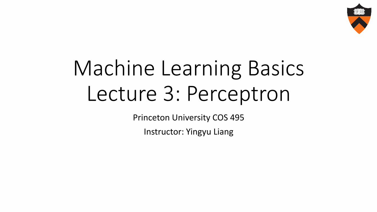
• Previous lectures: (Principle for loss function) MLE to derive loss• Example: linear regression; some linear classification models
• This lecture: (Principle for optimization) local improvement• Example: Perceptron; SGD
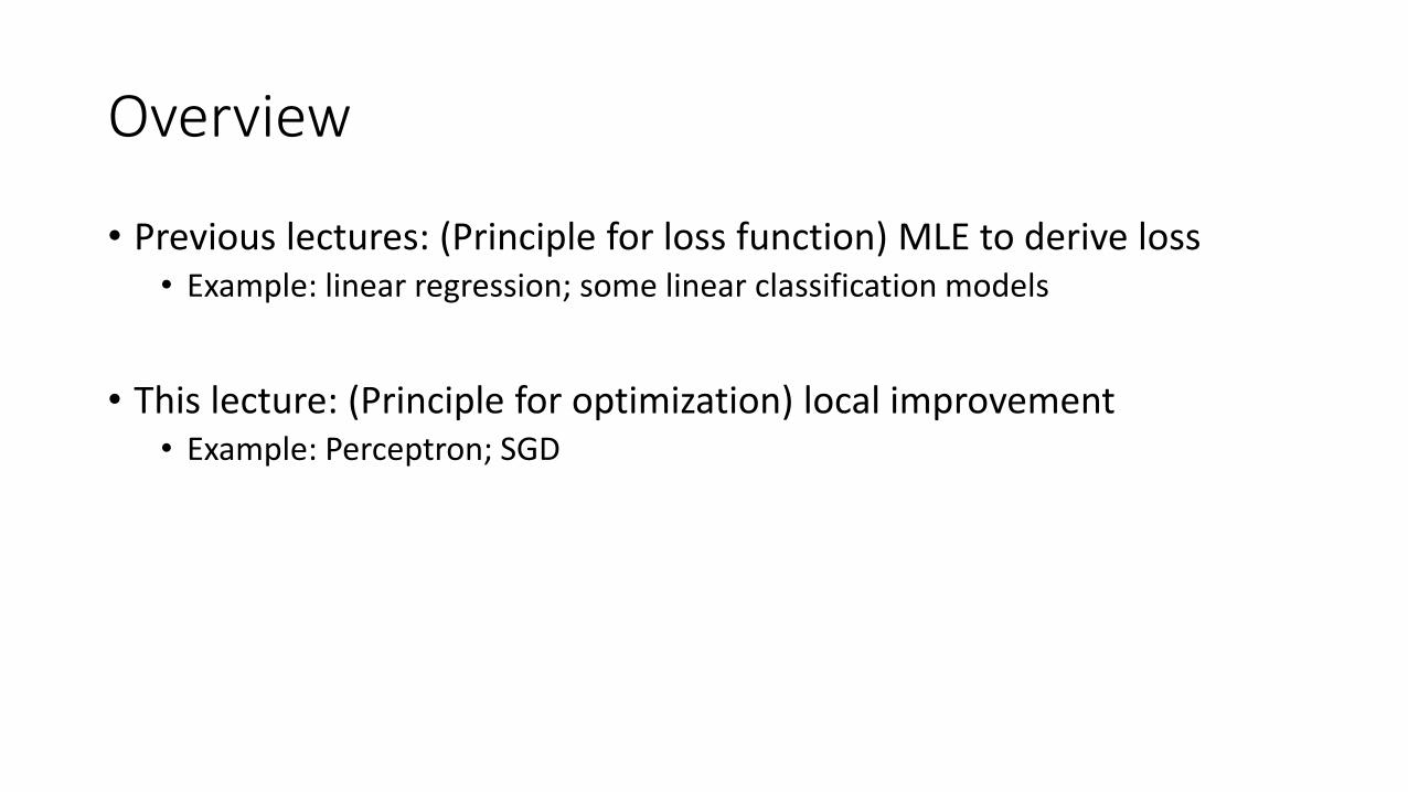
Task (𝑤∗)𝑇𝑥 = 0
Class +1
Class -1
𝑤∗
(𝑤∗)𝑇𝑥 > 0
(𝑤∗)𝑇𝑥 < 0
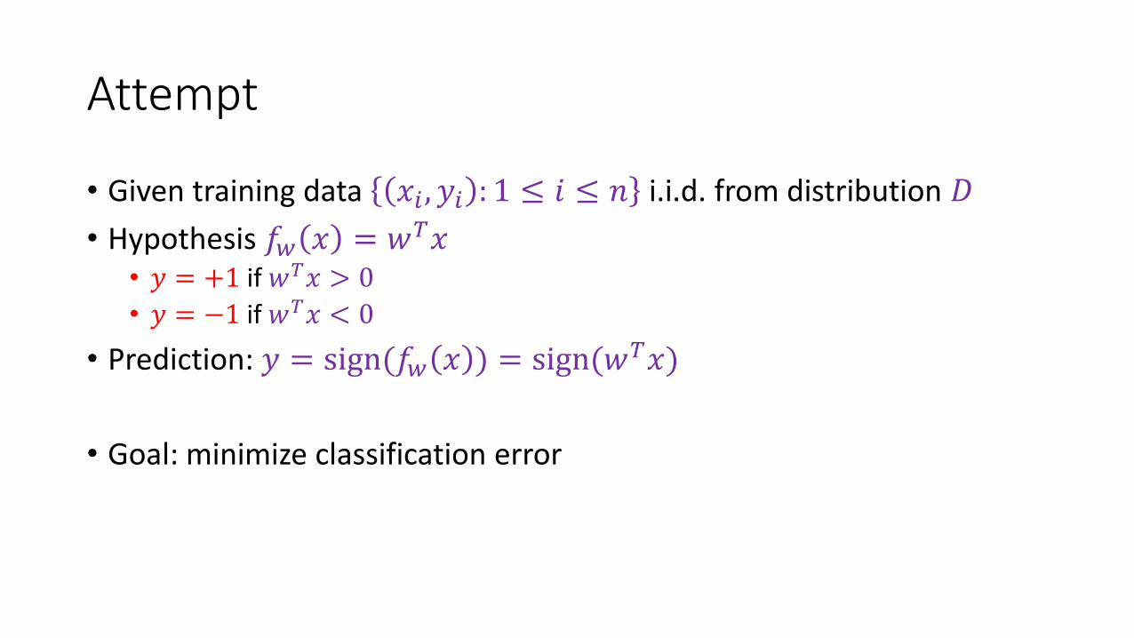
Attempt
• Given training data 𝑥𝑖 , 𝑦𝑖 : 1 ≤ 𝑖 ≤ 𝑛 i.i.d. from distribution 𝐷
• Hypothesis 𝑓𝑤 𝑥 = 𝑤𝑇𝑥• 𝑦 = +1 if 𝑤𝑇𝑥 > 0
• 𝑦 = −1 if 𝑤𝑇𝑥 < 0
• Prediction: 𝑦 = sign(𝑓𝑤 𝑥 ) = sign(𝑤𝑇𝑥)
• Goal: minimize classification error
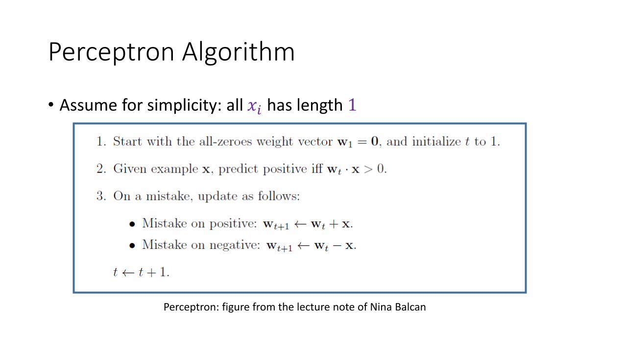
Perceptron Algorithm
• Assume for simplicity: all 𝑥𝑖 has length 1
Perceptron: figure from the lecture note of Nina Balcan
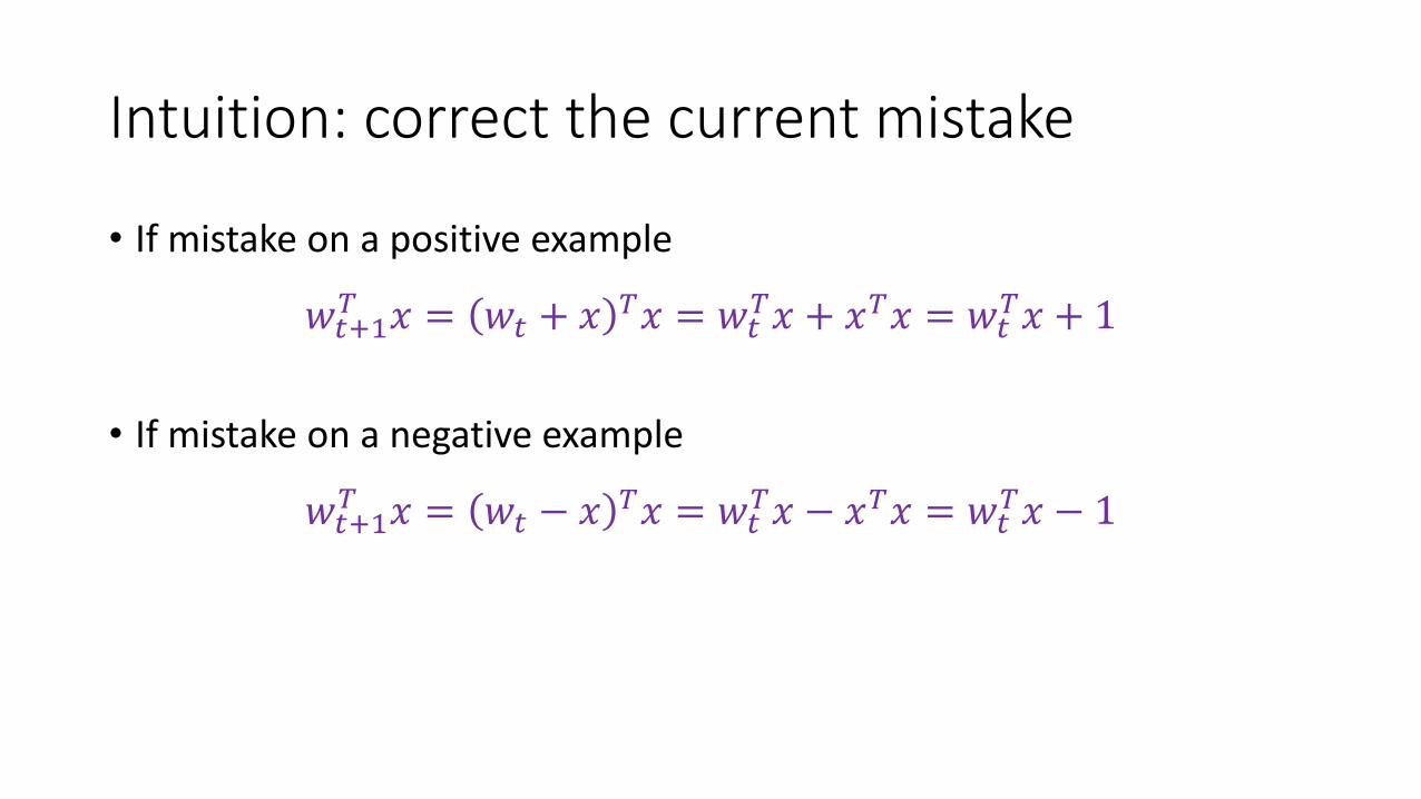
Intuition: correct the current mistake
• If mistake on a positive example
𝑤𝑡+1𝑇 𝑥 = 𝑤𝑡 + 𝑥 𝑇𝑥 = 𝑤𝑡
𝑇𝑥 + 𝑥𝑇𝑥 = 𝑤𝑡𝑇𝑥 + 1
• If mistake on a negative example
𝑤𝑡+1𝑇 𝑥 = 𝑤𝑡 − 𝑥 𝑇𝑥 = 𝑤𝑡
𝑇𝑥 − 𝑥𝑇𝑥 = 𝑤𝑡𝑇𝑥 − 1
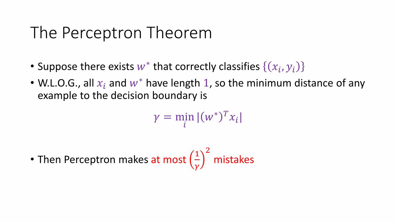
The Perceptron Theorem
• Suppose there exists 𝑤∗ that correctly classifies 𝑥𝑖 , 𝑦𝑖
• W.L.O.G., all 𝑥𝑖 and 𝑤∗ have length 1, so the minimum distance of any example to the decision boundary is
𝛾 = min𝑖
| 𝑤∗ 𝑇𝑥𝑖|
• Then Perceptron makes at most1
𝛾
2mistakes
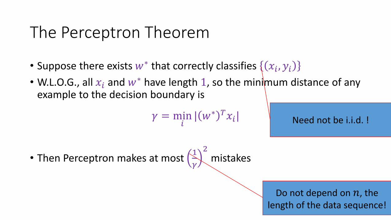
The Perceptron Theorem
• Suppose there exists 𝑤∗ that correctly classifies 𝑥𝑖 , 𝑦𝑖
• W.L.O.G., all 𝑥𝑖 and 𝑤∗ have length 1, so the minimum distance of any example to the decision boundary is
𝛾 = min𝑖
| 𝑤∗ 𝑇𝑥𝑖|
• Then Perceptron makes at most1
𝛾
2mistakes
Need not be i.i.d. !
Do not depend on 𝑛, the length of the data sequence!
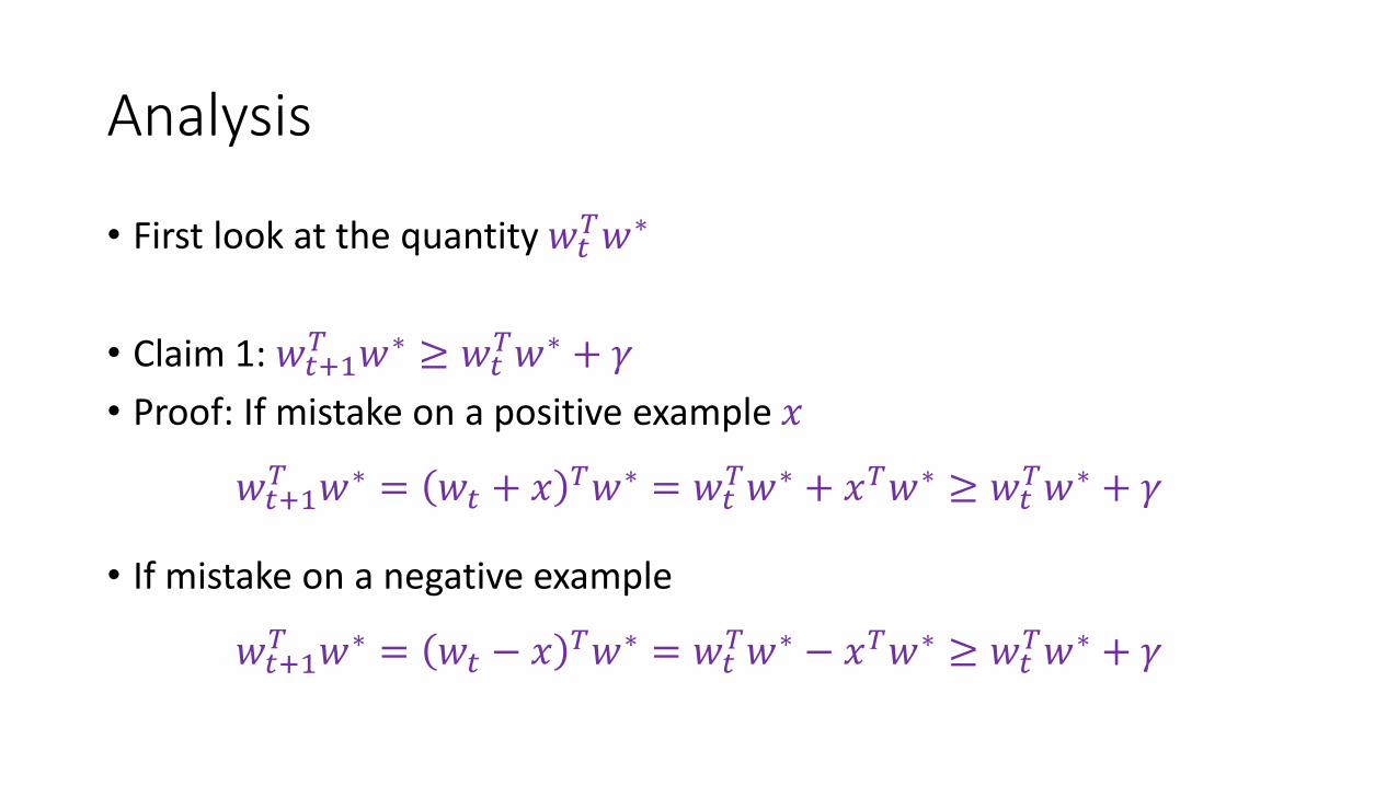
Analysis
• First look at the quantity 𝑤𝑡𝑇𝑤∗
• Claim 1: 𝑤𝑡+1𝑇 𝑤∗ ≥ 𝑤𝑡
𝑇𝑤∗ + 𝛾
• Proof: If mistake on a positive example 𝑥
𝑤𝑡+1𝑇 𝑤∗ = 𝑤𝑡 + 𝑥 𝑇𝑤∗ = 𝑤𝑡
𝑇𝑤∗ + 𝑥𝑇𝑤∗ ≥ 𝑤𝑡𝑇𝑤∗ + 𝛾
• If mistake on a negative example
𝑤𝑡+1𝑇 𝑤∗ = 𝑤𝑡 − 𝑥 𝑇𝑤∗ = 𝑤𝑡
𝑇𝑤∗ − 𝑥𝑇𝑤∗ ≥ 𝑤𝑡𝑇𝑤∗ + 𝛾
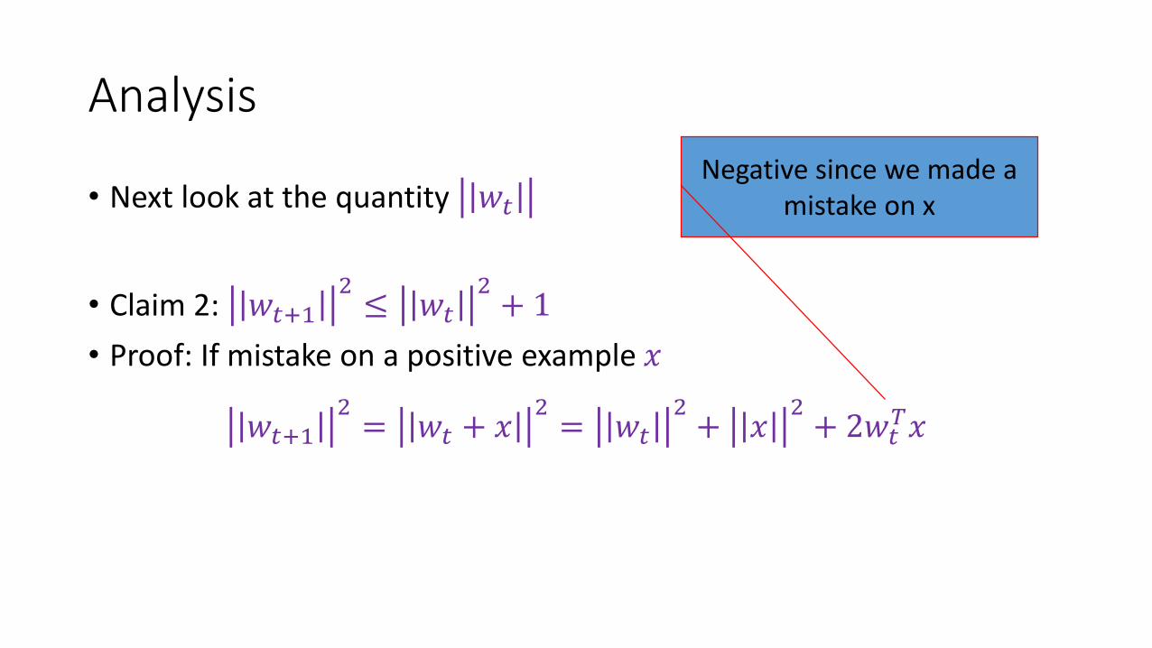
Analysis
• Next look at the quantity 𝑤𝑡
• Claim 2: 𝑤𝑡+12
≤ 𝑤𝑡2
+ 1
• Proof: If mistake on a positive example 𝑥
𝑤𝑡+12
= 𝑤𝑡 + 𝑥2
= 𝑤𝑡2
+ 𝑥2
+ 2𝑤𝑡𝑇𝑥
Negative since we made a mistake on x

Analysis: putting things together
• Claim 1: 𝑤𝑡+1𝑇 𝑤∗ ≥ 𝑤𝑡
𝑇𝑤∗ + 𝛾
• Claim 2: 𝑤𝑡+12
≤ 𝑤𝑡2
+ 1
After 𝑀 mistakes:
• 𝑤𝑀+1𝑇 𝑤∗ ≥ 𝛾𝑀
• 𝑤𝑀+1 ≤ √𝑀
• 𝑤𝑀+1𝑇 𝑤∗ ≤ 𝑤𝑀+1
So 𝛾𝑀 ≤ √𝑀, and thus 𝑀 ≤1
𝛾
2
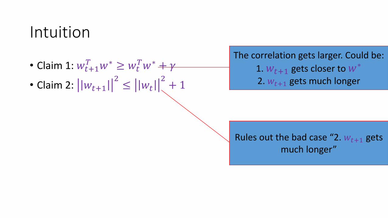
Intuition
• Claim 1: 𝑤𝑡+1𝑇 𝑤∗ ≥ 𝑤𝑡
𝑇𝑤∗ + 𝛾
• Claim 2: 𝑤𝑡+12
≤ 𝑤𝑡2
+ 1
The correlation gets larger. Could be:
1. 𝑤𝑡+1 gets closer to 𝑤∗
2. 𝑤𝑡+1 gets much longer
Rules out the bad case “2. 𝑤𝑡+1 gets much longer”

Some side notes on Perceptron

History
Figure from Pattern Recognition and Machine Learning, Bishop

Note: connectionism vs symbolism
• Symbolism: AI can be achieved by representing concepts as symbols• Example: rule-based expert system, formal grammar
• Connectionism: explain intellectual abilities using connections between neurons (i.e., artificial neural networks)• Example: perceptron, larger scale neural networks
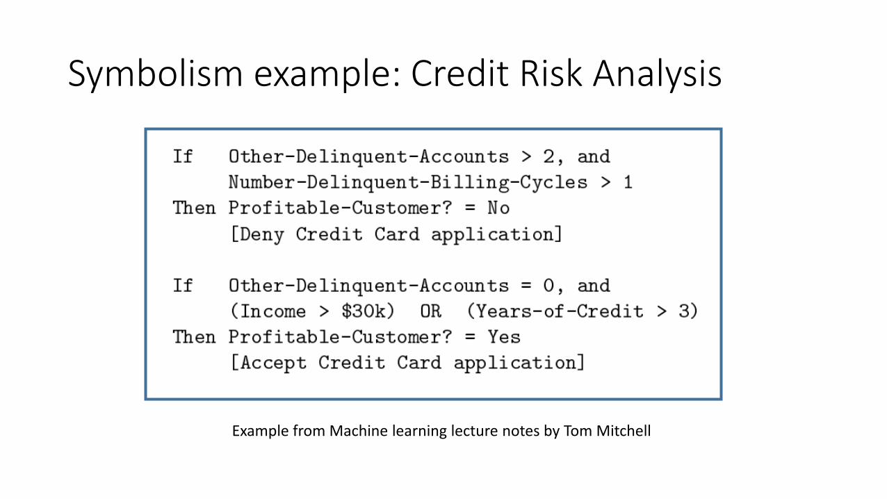
Symbolism example: Credit Risk Analysis
Example from Machine learning lecture notes by Tom Mitchell
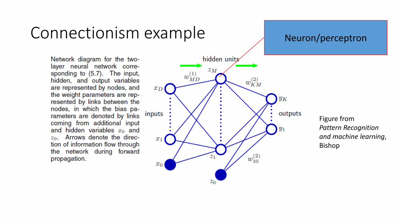
Connectionism example
Figure from Pattern Recognitionand machine learning,Bishop
Neuron/perceptron
Note: connectionism v.s. symbolism
• Formal theories of logical reasoning, grammar, and other higher mental faculties compel us to think of the mind as a machine for rule-based manipulation of highly structured arrays of symbols. What we know of the brain compels us to think of human information processing in terms of manipulation of a large unstructured set of numbers, the activity levels of interconnected neurons.
---- The Central Paradox of Cognition (Smolensky et al., 1992)

Note: online vs batch
• Batch: Given training data 𝑥𝑖 , 𝑦𝑖 : 1 ≤ 𝑖 ≤ 𝑛 , typically i.i.d.
• Online: data points arrive one by one• 1. The algorithm receives an unlabeled example 𝑥𝑖
• 2. The algorithm predicts a classification of this example.
• 3. The algorithm is then told the correct answer 𝑦𝑖, and update its model

Stochastic gradient descent (SGD)
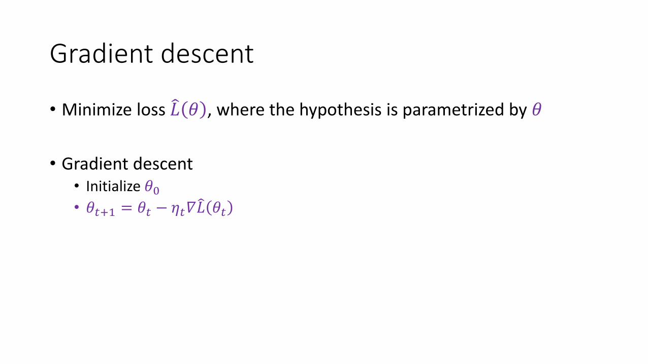
Gradient descent
• Minimize loss 𝐿 𝜃 , where the hypothesis is parametrized by 𝜃
• Gradient descent• Initialize 𝜃0
• 𝜃𝑡+1 = 𝜃𝑡 − 𝜂𝑡𝛻 𝐿 𝜃𝑡
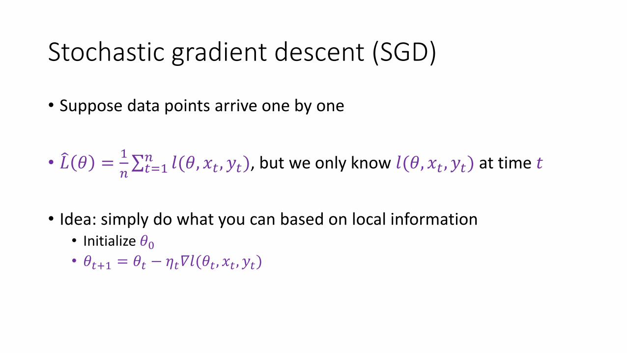
Stochastic gradient descent (SGD)
• Suppose data points arrive one by one
• 𝐿 𝜃 =1
𝑛σ𝑡=1
𝑛 𝑙(𝜃, 𝑥𝑡 , 𝑦𝑡), but we only know 𝑙(𝜃, 𝑥𝑡 , 𝑦𝑡) at time 𝑡
• Idea: simply do what you can based on local information• Initialize 𝜃0
• 𝜃𝑡+1 = 𝜃𝑡 − 𝜂𝑡𝛻𝑙(𝜃𝑡, 𝑥𝑡 , 𝑦𝑡)

Example 1: linear regression
• Find 𝑓𝑤 𝑥 = 𝑤𝑇𝑥 that minimizes 𝐿 𝑓𝑤 =1
𝑛σ𝑡=1
𝑛 𝑤𝑇𝑥𝑡 − 𝑦𝑡2
• 𝑙 𝑤, 𝑥𝑡 , 𝑦𝑡 =1
𝑛𝑤𝑇𝑥𝑡 − 𝑦𝑡
2
• 𝑤𝑡+1 = 𝑤𝑡 − 𝜂𝑡𝛻𝑙 𝑤𝑡 , 𝑥𝑡 , 𝑦𝑡 = 𝑤𝑡 −2𝜂𝑡
𝑛𝑤𝑡
𝑇𝑥𝑡 − 𝑦𝑡 𝑥𝑡

Example 2: logistic regression
• Find 𝑤 that minimizes
𝐿 𝑤 = −1
𝑛
𝑦𝑡=1
log𝜎(𝑤𝑇𝑥𝑡) −1
𝑛
𝑦𝑡=−1
log[1 − 𝜎 𝑤𝑇𝑥𝑡 ]
𝐿 𝑤 = −1
𝑛
𝑡
log𝜎(𝑦𝑡𝑤𝑇𝑥𝑡)
𝑙 𝑤, 𝑥𝑡 , 𝑦𝑡 =−1
𝑛log𝜎(𝑦𝑡𝑤𝑇𝑥𝑡)
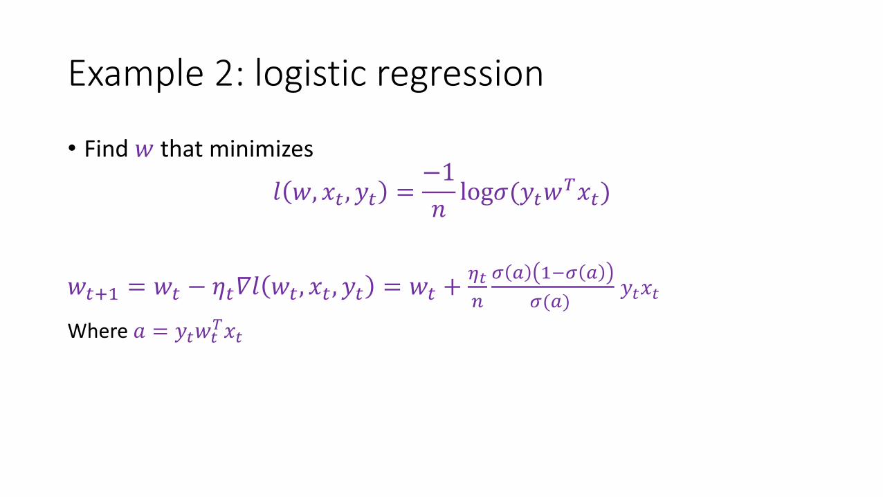
Example 2: logistic regression
• Find 𝑤 that minimizes
𝑙 𝑤, 𝑥𝑡 , 𝑦𝑡 =−1
𝑛log𝜎(𝑦𝑡𝑤𝑇𝑥𝑡)
𝑤𝑡+1 = 𝑤𝑡 − 𝜂𝑡𝛻𝑙 𝑤𝑡 , 𝑥𝑡 , 𝑦𝑡 = 𝑤𝑡 +𝜂𝑡
𝑛
𝜎 𝑎 1−𝜎 𝑎
𝜎(𝑎)𝑦𝑡𝑥𝑡
Where 𝑎 = 𝑦𝑡𝑤𝑡𝑇𝑥𝑡
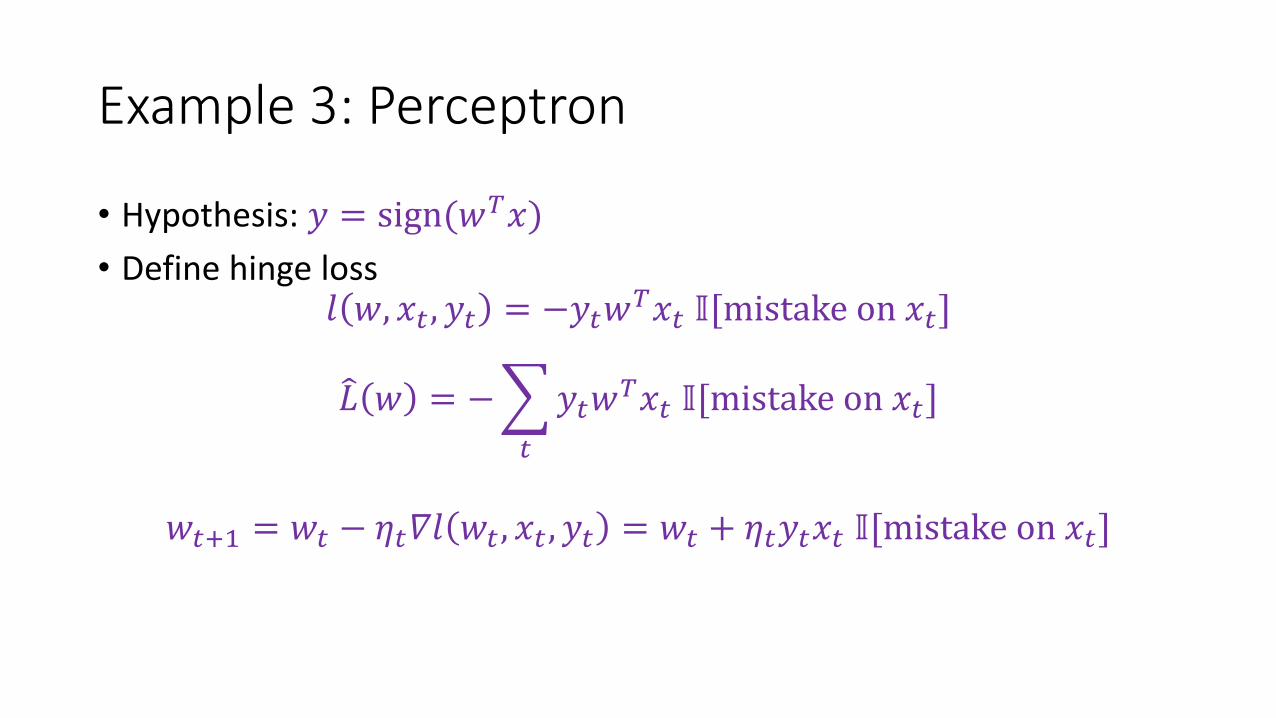
Example 3: Perceptron
• Hypothesis: 𝑦 = sign(𝑤𝑇𝑥)
• Define hinge loss𝑙 𝑤, 𝑥𝑡 , 𝑦𝑡 = −𝑦𝑡𝑤𝑇𝑥𝑡 𝕀[mistake on 𝑥𝑡]
𝐿 𝑤 = −
𝑡
𝑦𝑡𝑤𝑇𝑥𝑡 𝕀[mistake on 𝑥𝑡]
𝑤𝑡+1 = 𝑤𝑡 − 𝜂𝑡𝛻𝑙 𝑤𝑡 , 𝑥𝑡 , 𝑦𝑡 = 𝑤𝑡 + 𝜂𝑡𝑦𝑡𝑥𝑡 𝕀[mistake on 𝑥𝑡]
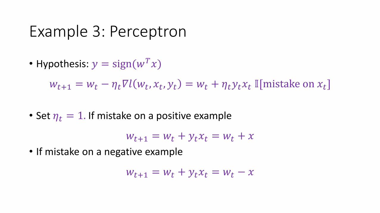
Example 3: Perceptron
• Hypothesis: 𝑦 = sign(𝑤𝑇𝑥)
𝑤𝑡+1 = 𝑤𝑡 − 𝜂𝑡𝛻𝑙 𝑤𝑡 , 𝑥𝑡 , 𝑦𝑡 = 𝑤𝑡 + 𝜂𝑡𝑦𝑡𝑥𝑡 𝕀[mistake on 𝑥𝑡]
• Set 𝜂𝑡 = 1. If mistake on a positive example
𝑤𝑡+1 = 𝑤𝑡 + 𝑦𝑡𝑥𝑡 = 𝑤𝑡 + 𝑥
• If mistake on a negative example
𝑤𝑡+1 = 𝑤𝑡 + 𝑦𝑡𝑥𝑡 = 𝑤𝑡 − 𝑥
Pros & Cons
Pros:
• Widely applicable
• Easy to implement in most cases
• Guarantees for many losses
• Good performance: error/running time/memory etc.
Cons:
• No guarantees for non-convex opt (e.g., those in deep learning)
• Hyper-parameters: initialization, learning rate
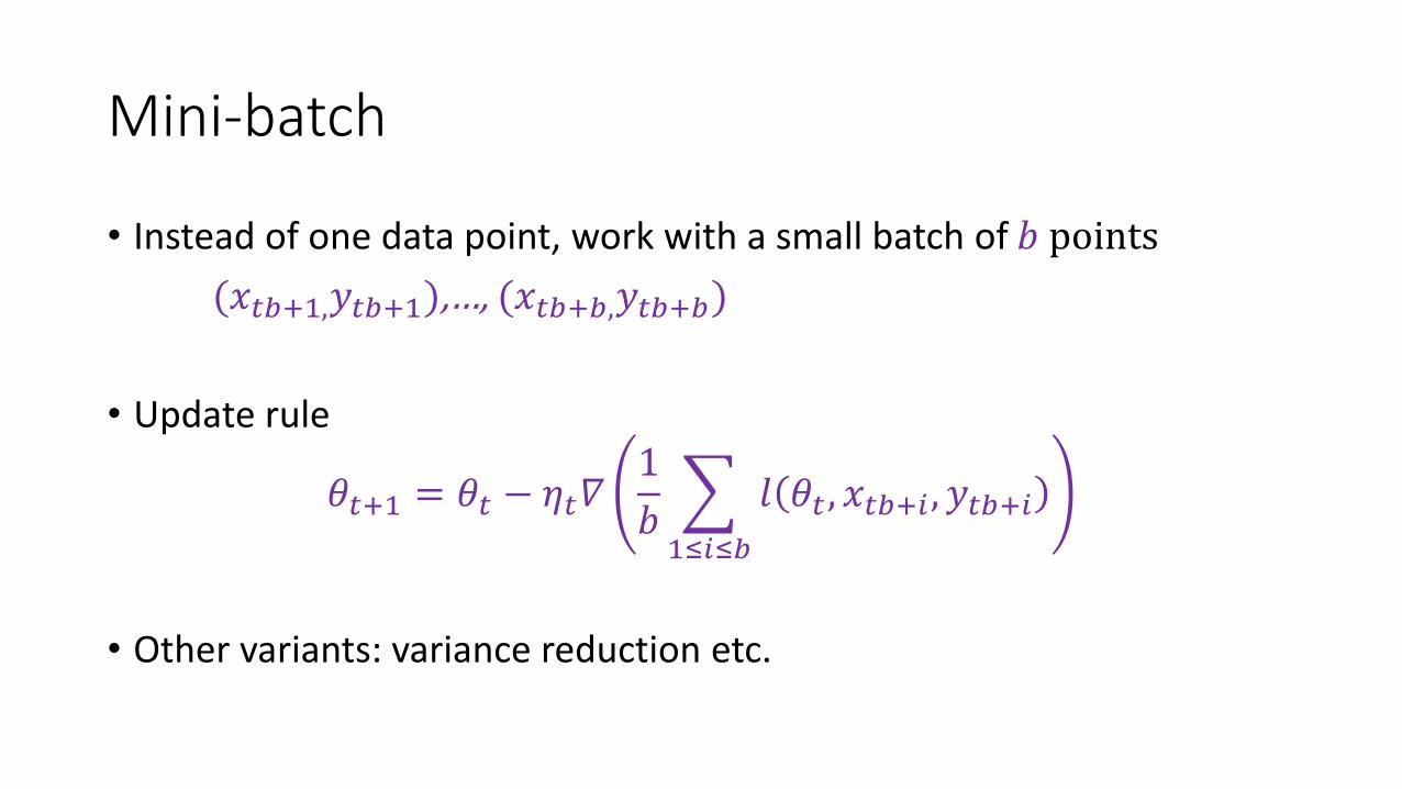
Mini-batch
• Instead of one data point, work with a small batch of 𝑏 points
(𝑥𝑡𝑏+1,𝑦𝑡𝑏+1),…, (𝑥𝑡𝑏+𝑏,𝑦𝑡𝑏+𝑏)
• Update rule
𝜃𝑡+1 = 𝜃𝑡 − 𝜂𝑡𝛻1
𝑏
1≤𝑖≤𝑏
𝑙 𝜃𝑡 , 𝑥𝑡𝑏+𝑖 , 𝑦𝑡𝑏+𝑖
• Other variants: variance reduction etc.

Homework

Homework 1
• Assignment online• Course website:
http://www.cs.princeton.edu/courses/archive/spring16/cos495/
• Piazza: https://piazza.com/princeton/spring2016/cos495
• Due date: Feb 17th (one week)
• Submission• Math part: hand-written/print; submit to TA (Office: EE, C319B)
• Coding part: in Matlab/Python; submit the .m/.py file on Piazza

Homework 1
• Grading policy: every late day reduces the attainable credit for the exercise by 10%.
• Collaboration: • Discussion on the problem sets is allowed
• Students are expected to finish the homework by himself/herself
• The people you discussed with on assignments should be clearly detailed: before the solution to each question, list all people that you discussed with on that particular question.


![Gov 2002: 7. Regression and Causality• Define linear regression: =argmin 𝔼[( 𝑖− ′ ) ] • The solution to this is the following: =𝔼[ 𝑖 ′]− 𝔼[ 𝑖 𝑖] •](https://img.pdfslide.net/doc/110x75/604f45529079573162360e46/gov-2002-7-regression-and-causality-a-define-linear-regression-argmin-.jpg)