Machine Learning & Data Mining CS/CNS/EE 155 Lecture 6: Conditional Random Fields 1

1

Machine Learning & Data MiningCS/CNS/EE 155

Lecture 6:Conditional Random Fields

2

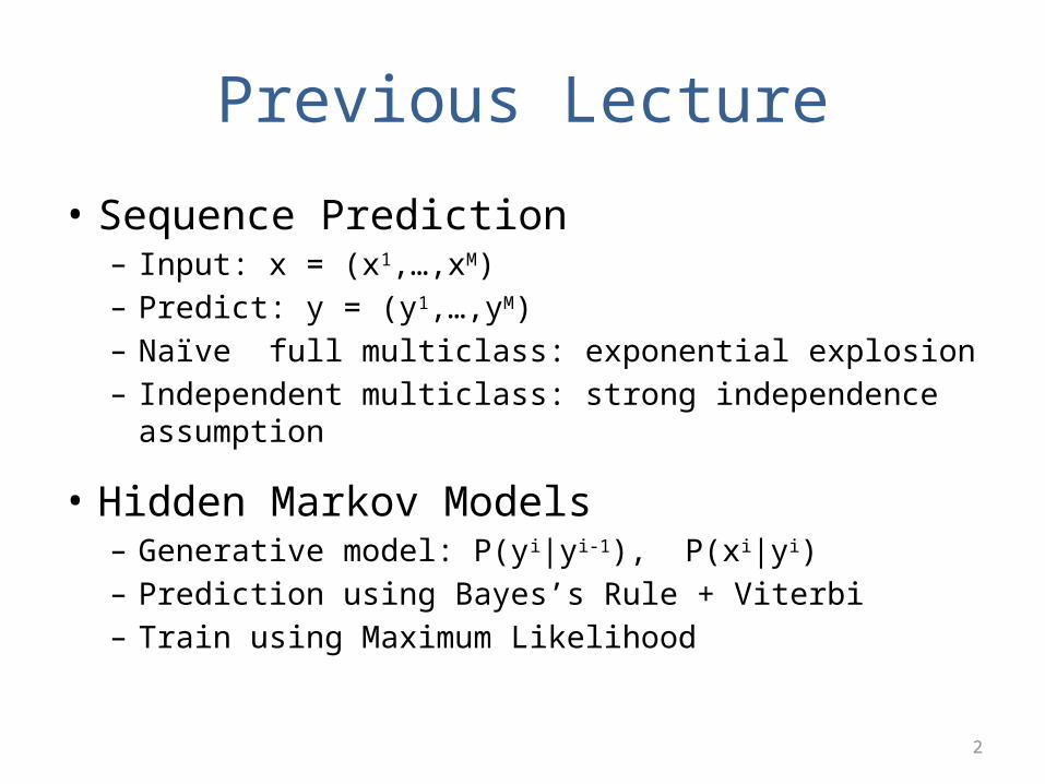
Previous Lecture

• Sequence Prediction– Input: x = (x1,…,xM)– Predict: y = (y1,…,yM)– Naïve full multiclass: exponential explosion– Independent multiclass: strong independence assumption

• Hidden Markov Models– Generative model: P(yi|yi-1), P(xi|yi)– Prediction using Bayes’s Rule + Viterbi– Train using Maximum Likelihood

3

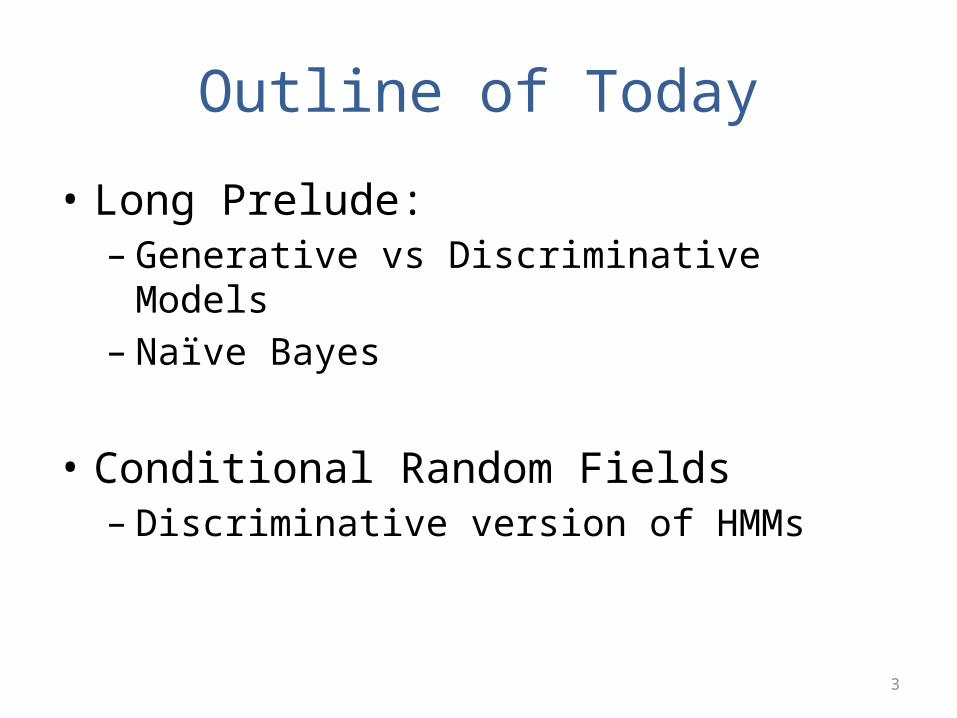
Outline of Today

• Long Prelude: – Generative vs Discriminative Models– Naïve Bayes

• Conditional Random Fields– Discriminative version of HMMs

4

Generative vs Discriminative

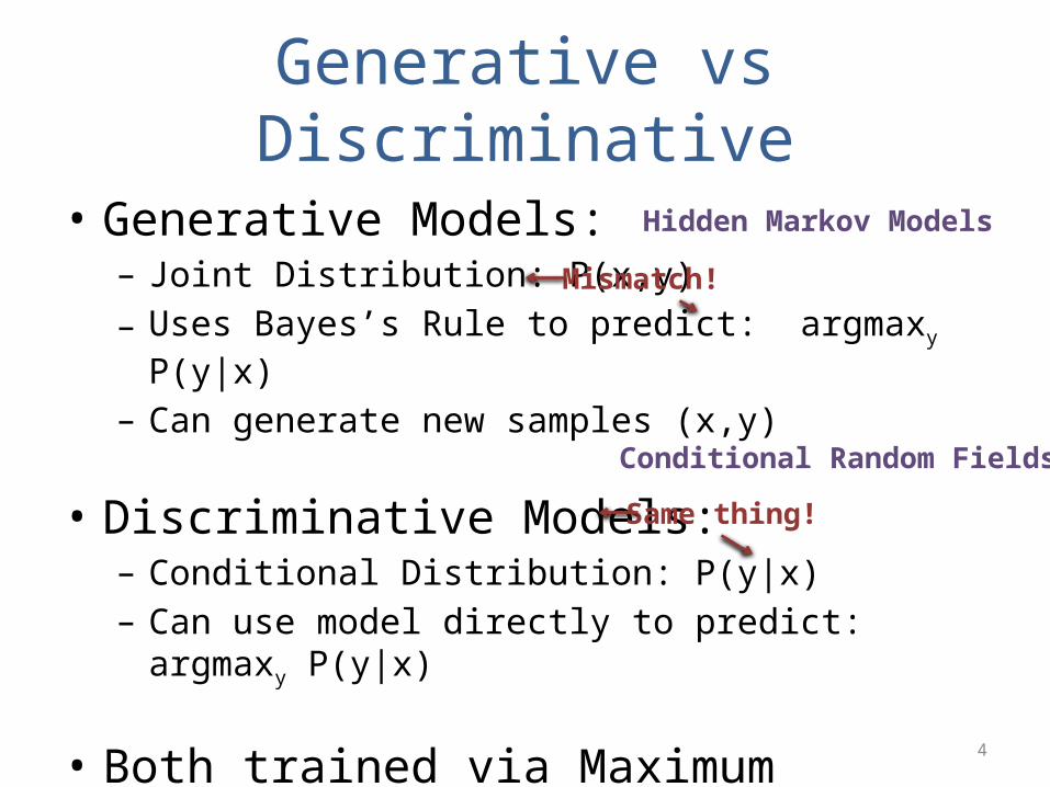
• Generative Models:– Joint Distribution: P(x,y)– Uses Bayes’s Rule to predict: argmaxy P(y|x)– Can generate new samples (x,y)

• Discriminative Models:– Conditional Distribution: P(y|x)– Can use model directly to predict: argmaxy P(y|x)

• Both trained via Maximum Likelihood

Same thing!

Hidden Markov Models

Conditional Random Fields

Mismatch!

5

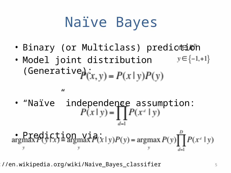
Naïve Bayes

• Binary (or Multiclass) prediction• Model joint distribution (Generative):

• “Naïve” independence assumption:

• Prediction via:

http://en.wikipedia.org/wiki/Naive_Bayes_classifier

6

Naïve Bayes

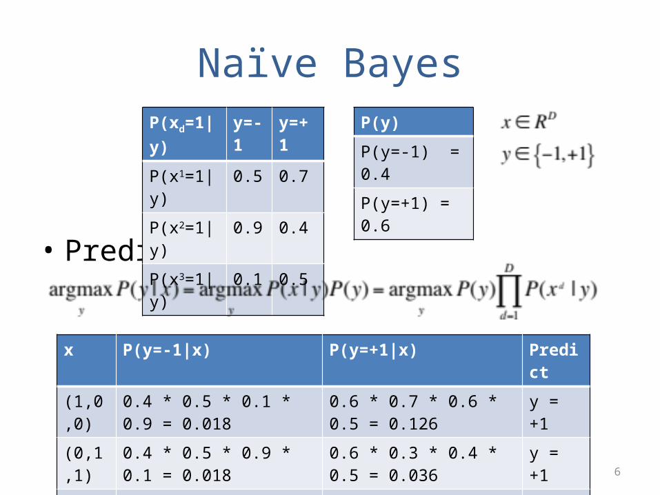
• Prediction:

P(xd=1|y) y=-1 y=+1

P(x1=1|y) 0.5 0.7P(x2=1|y) 0.9 0.4P(x3=1|y) 0.1 0.5

P(y)

P(y=-1) = 0.4

P(y=+1) = 0.6

x P(y=-1|x) P(y=+1|x) Predict

(1,0,0) 0.4 * 0.5 * 0.1 * 0.9 = 0.018 0.6 * 0.7 * 0.6 * 0.5 = 0.126 y = +1

(0,1,1) 0.4 * 0.5 * 0.9 * 0.1 = 0.018 0.6 * 0.3 * 0.4 * 0.5 = 0.036 y = +1

(0,1,0) 0.4 * 0.5 * 0.9 * 0.9 = 0.162 0.6 * 0.3 * 0.4 * 0.5 = 0.036 y = -1

7

Naïve Bayes

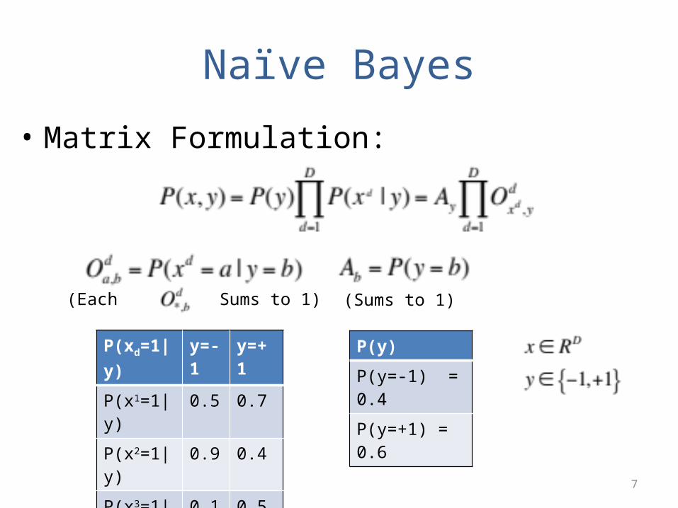
• Matrix Formulation:

P(xd=1|y) y=-1 y=+1

P(x1=1|y) 0.5 0.7P(x2=1|y) 0.9 0.4P(x3=1|y) 0.1 0.5

P(y)

P(y=-1) = 0.4

P(y=+1) = 0.6

(Sums to 1)(Each Sums to 1)

8

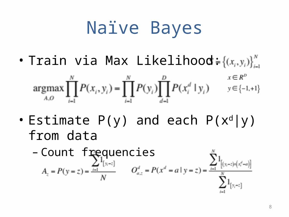
Naïve Bayes

• Train via Max Likelihood:

• Estimate P(y) and each P(xd|y) from data– Count frequencies

9

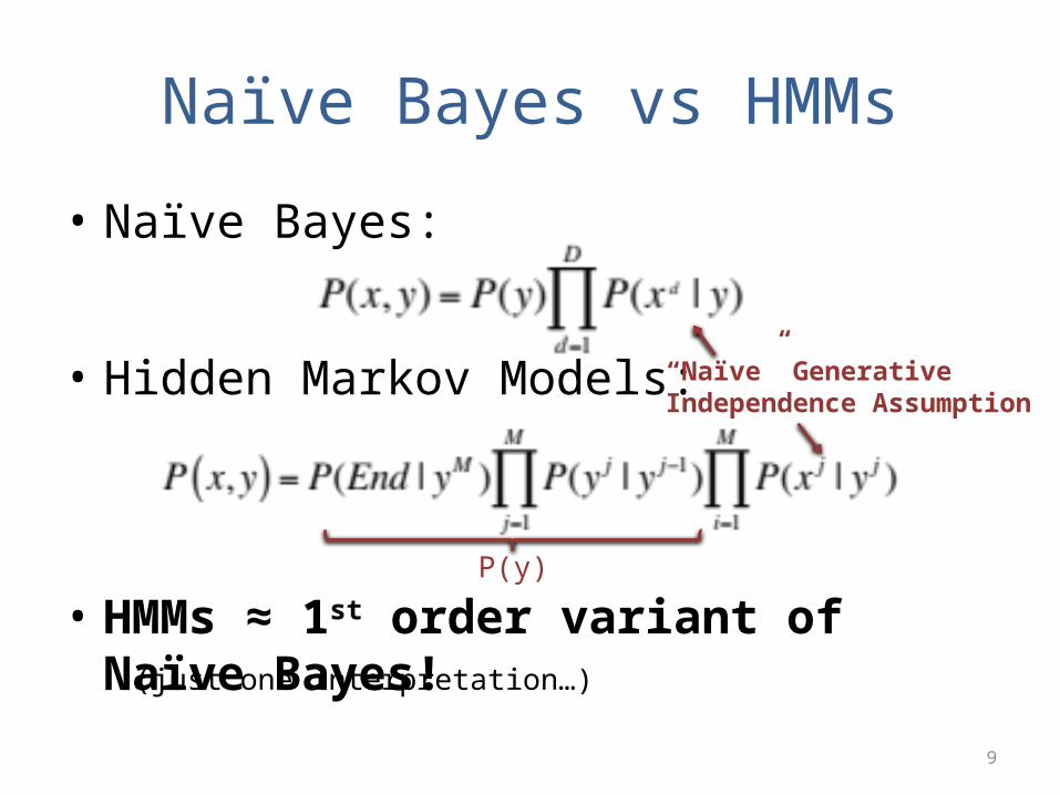
Naïve Bayes vs HMMs

• Naïve Bayes:

• Hidden Markov Models:

• HMMs ≈ 1st order variant of Naïve Bayes!

“Naïve” GenerativeIndependence Assumption

(just one interpretation…)

P(y)

10

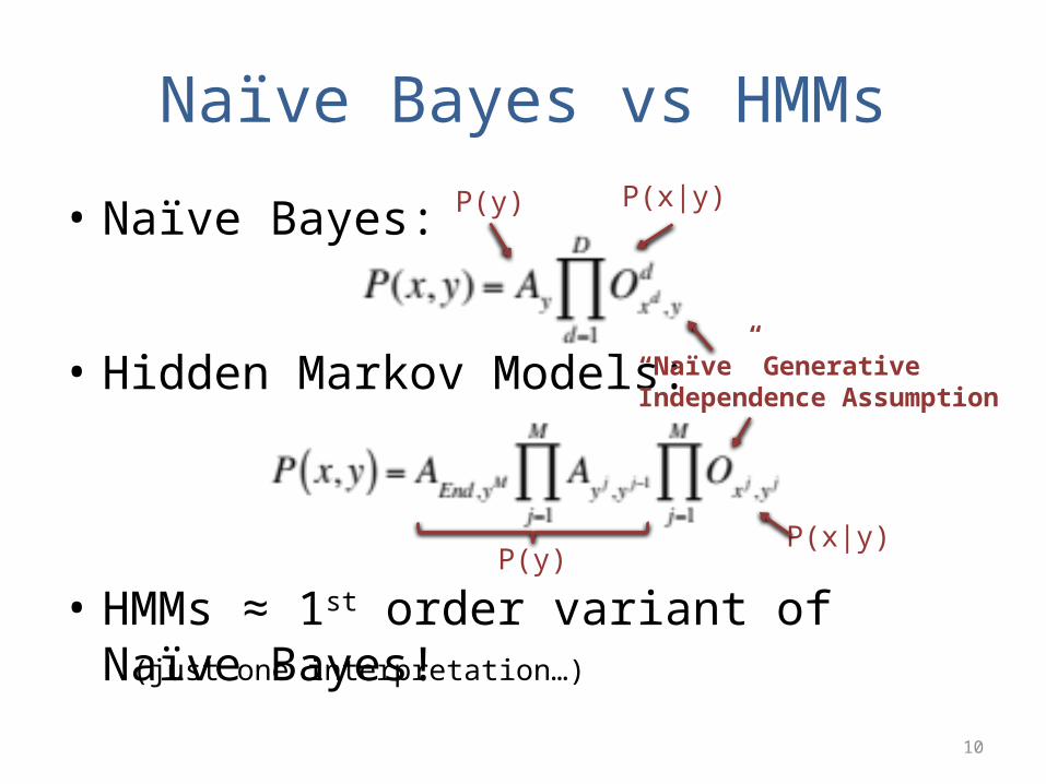
Naïve Bayes vs HMMs

• Naïve Bayes:

• Hidden Markov Models:

• HMMs ≈ 1st order variant of Naïve Bayes!(just one interpretation…)

P(y)

P(y)

“Naïve” GenerativeIndependence Assumption

P(x|y)

P(x|y)

11

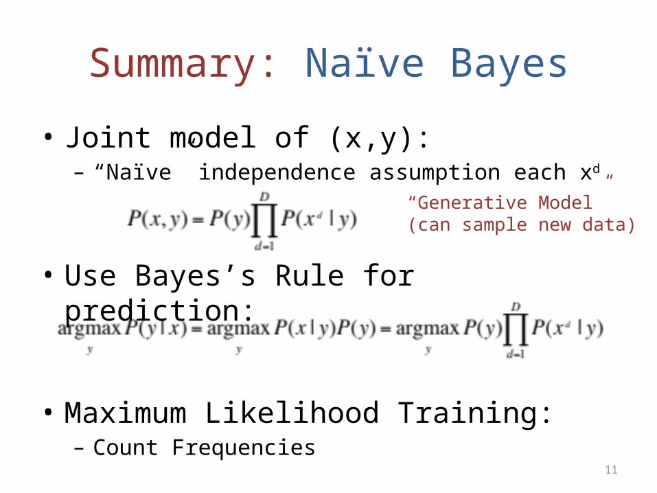
Summary: Naïve Bayes

• Joint model of (x,y):– “Naïve” independence assumption each xd

• Use Bayes’s Rule for prediction:

• Maximum Likelihood Training:– Count Frequencies

“Generative Model”(can sample new data)

12

Learn Conditional Prob.?

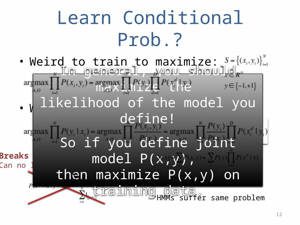
• Weird to train to maximize:

• When goal should be to maximize:

Breaks independence!Can no longer use count statistics

*HMMs suffer same problem

In general, you should maximize the likelihood of the model you define!

So if you define joint model P(x,y), then maximize P(x,y) on training data.

13

Summary: Generative Models

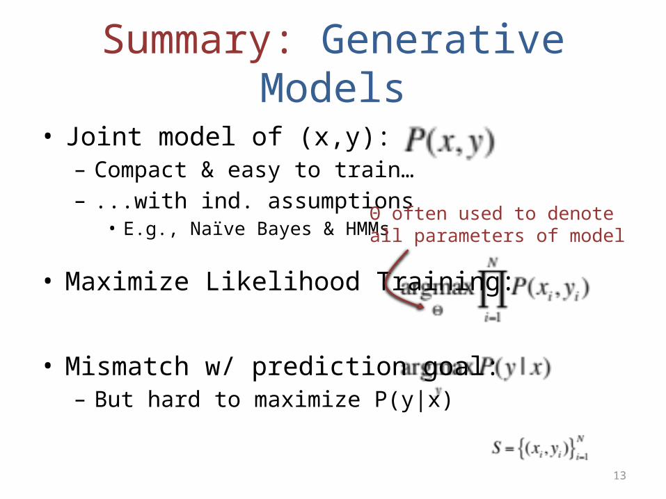
• Joint model of (x,y):– Compact & easy to train…– ...with ind. assumptions

• E.g., Naïve Bayes & HMMs

• Maximize Likelihood Training:

• Mismatch w/ prediction goal:– But hard to maximize P(y|x)

Θ often used to denote all parameters of model

14

Discriminative Models

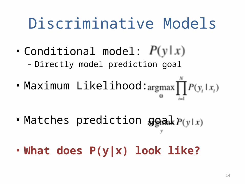
• Conditional model:– Directly model prediction goal

• Maximum Likelihood:

• Matches prediction goal:

• What does P(y|x) look like?

15

First Try

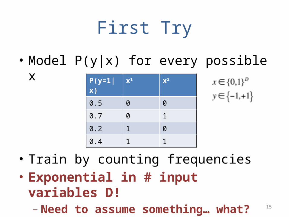
• Model P(y|x) for every possible x

• Train by counting frequencies• Exponential in # input variables D!– Need to assume something… what?

P(y=1|x) x1 x2

0.5 0 0

0.7 0 1

0.2 1 0

0.4 1 1

16

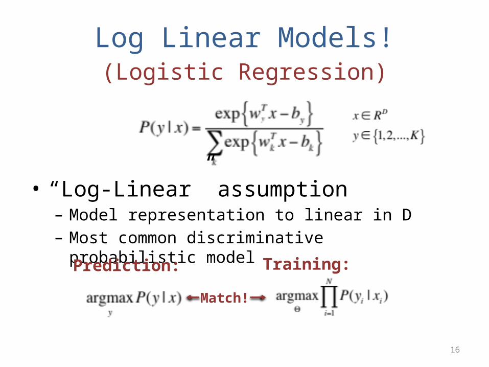
Log Linear Models!(Logistic Regression)

• “Log-Linear” assumption– Model representation to linear in D– Most common discriminative probabilistic model

Prediction: Training:

Match!

17

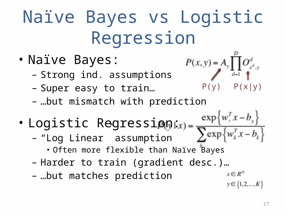
Naïve Bayes vs Logistic Regression

• Naïve Bayes:– Strong ind. assumptions– Super easy to train…– …but mismatch with prediction

• Logistic Regression:– “Log Linear” assumption

• Often more flexible than Naïve Bayes

– Harder to train (gradient desc.)…– …but matches prediction

P(y) P(x|y)

18

Naïve Bayes vs Logistic Regression

• NB has K parameters for P(y) (i.e., A)• LR has K parameters for bias b• NB has K*D parameters for P(x|y) (i.e, O)• LR has K*D parameters for w• Same number of parameters!

P(y) P(x|y)

Naïve Bayes Logistic Regression

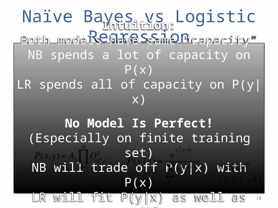
Intuition:Both models have same “capacity”NB spends a lot of capacity on P(x)LR spends all of capacity on P(y|x)

No Model Is Perfect!(Especially on finite training set)NB will trade off P(y|x) with P(x)

LR will fit P(y|x) as well as possible

19

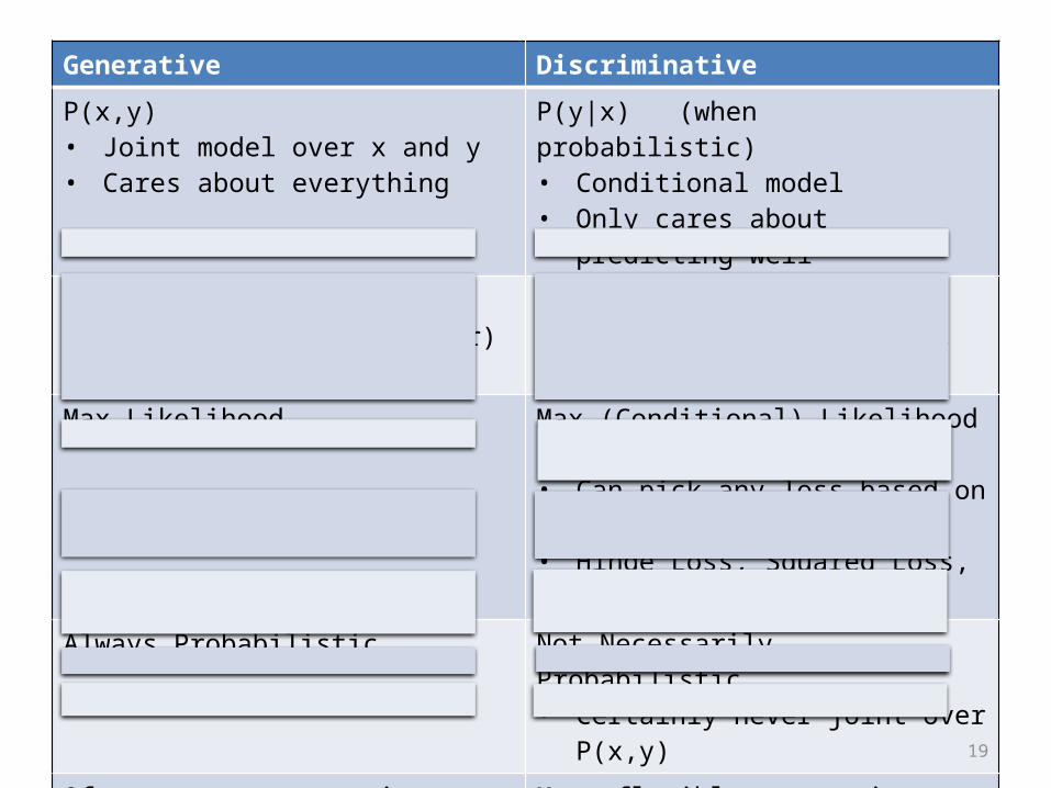
Generative Discriminative

P(x,y)• Joint model over x and y• Cares about everything

P(y|x) (when probabilistic)• Conditional model• Only cares about predicting well

Naïve Bayes, HMMs• Also Topic Models (later)

Logistic Regression, CRFs• also SVM, Least Squares, etc.

Max Likelihood Max (Conditional) Likelihood• (=minimize log loss)• Can pick any loss based on y• Hinge Loss, Squared Loss, etc.

Always Probabilistic Not Necessarily Probabilistic• Certainly never joint over P(x,y)

Often strong assumptions• Keeps training tractable

More flexible assumptions• Focuses entire model on P(y|x)

Mismatch between train & predict• Requires Bayes’s rule

Train to optimize predict goal

Can sample anything Can only sample y given x

Can handle missing values in x Cannot handle missing values in x

20

Conditional Random Fields

21

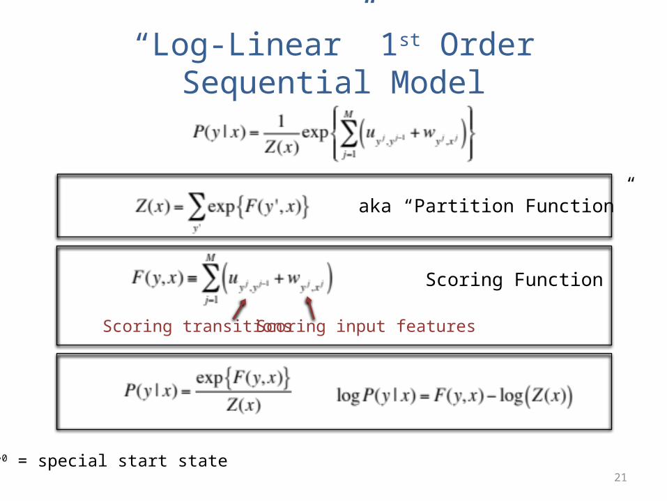
“Log-Linear” 1st Order Sequential Model

y0 = special start state

Scoring transitions Scoring input features

Scoring Function

aka “Partition Function”

22

( )

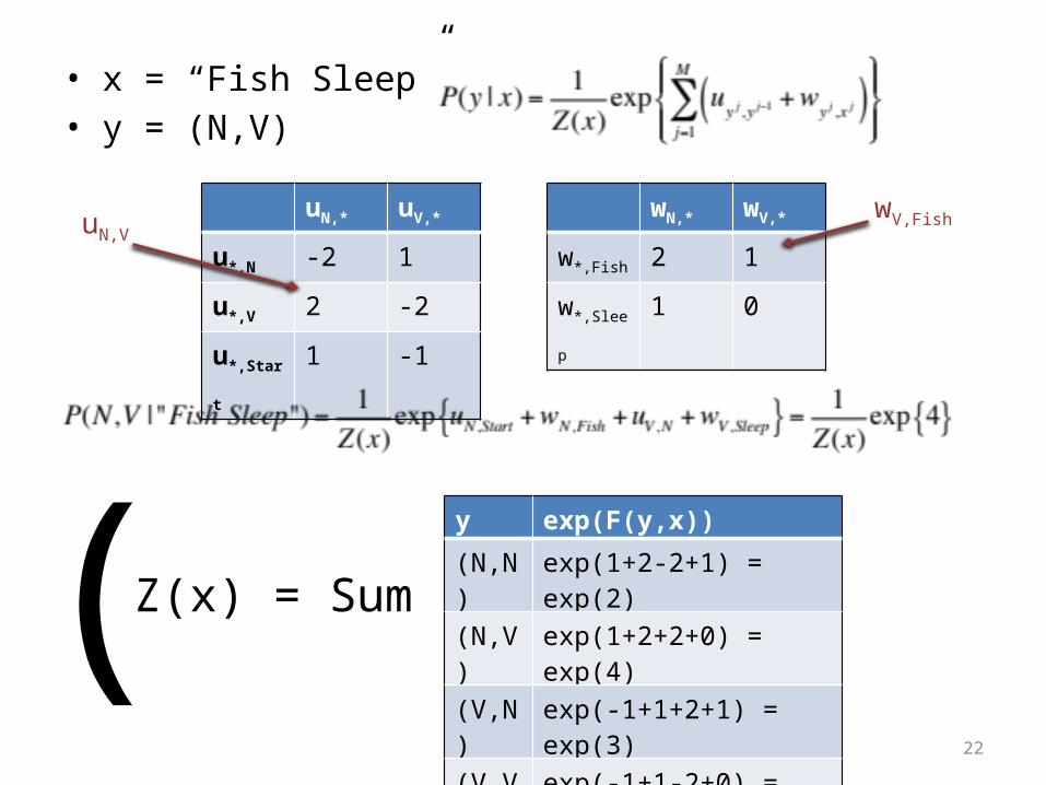
• x = “Fish Sleep”• y = (N,V)

uN,* uV,*

u*,N -2 1

u*,V 2 -2

u*,Start 1 -1

wN,* wV,*

w*,Fish 2 1

w*,Sleep 1 0

uN,VwV,Fish

y exp(F(y,x))

(N,N) exp(1+2-2+1) = exp(2)

(N,V) exp(1+2+2+0) = exp(4)

(V,N) exp(-1+1+2+1) = exp(3)

(V,V) exp(-1+1-2+0) = exp(-2)

Z(x) = Sum

23

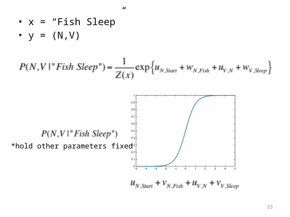
• x = “Fish Sleep”• y = (N,V)

*hold other parameters fixed

24

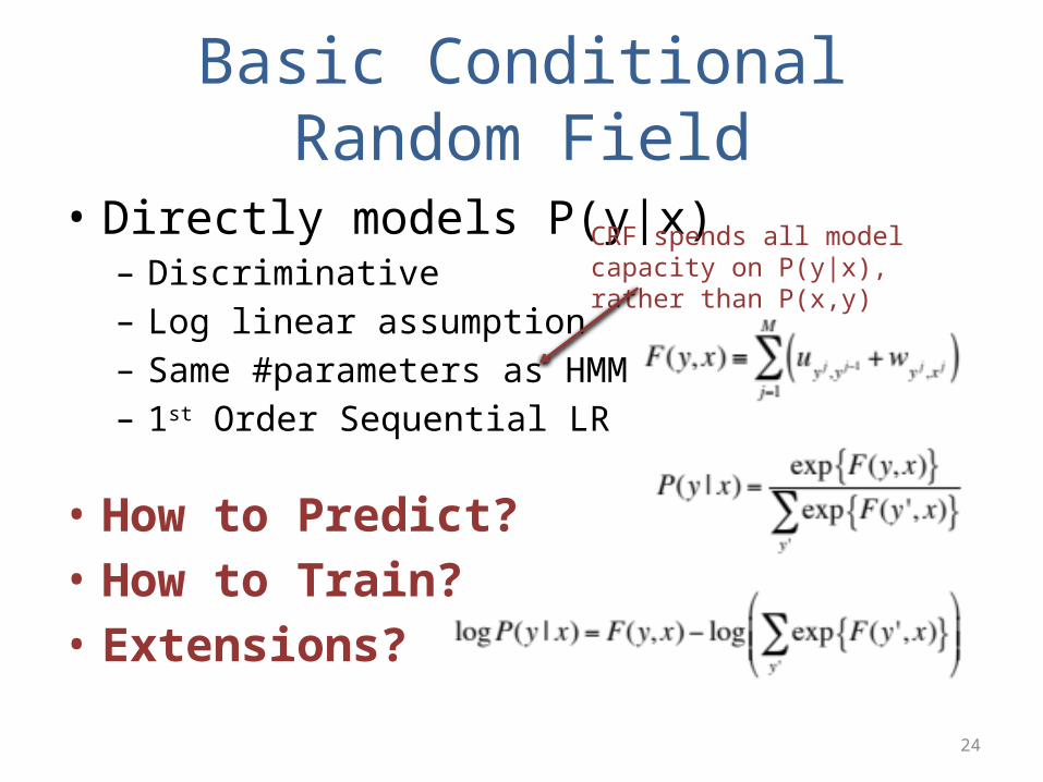
Basic Conditional Random Field

• Directly models P(y|x)– Discriminative – Log linear assumption– Same #parameters as HMM– 1st Order Sequential LR

• How to Predict?• How to Train?• Extensions?

CRF spends all model capacity on P(y|x), rather than P(x,y)

25

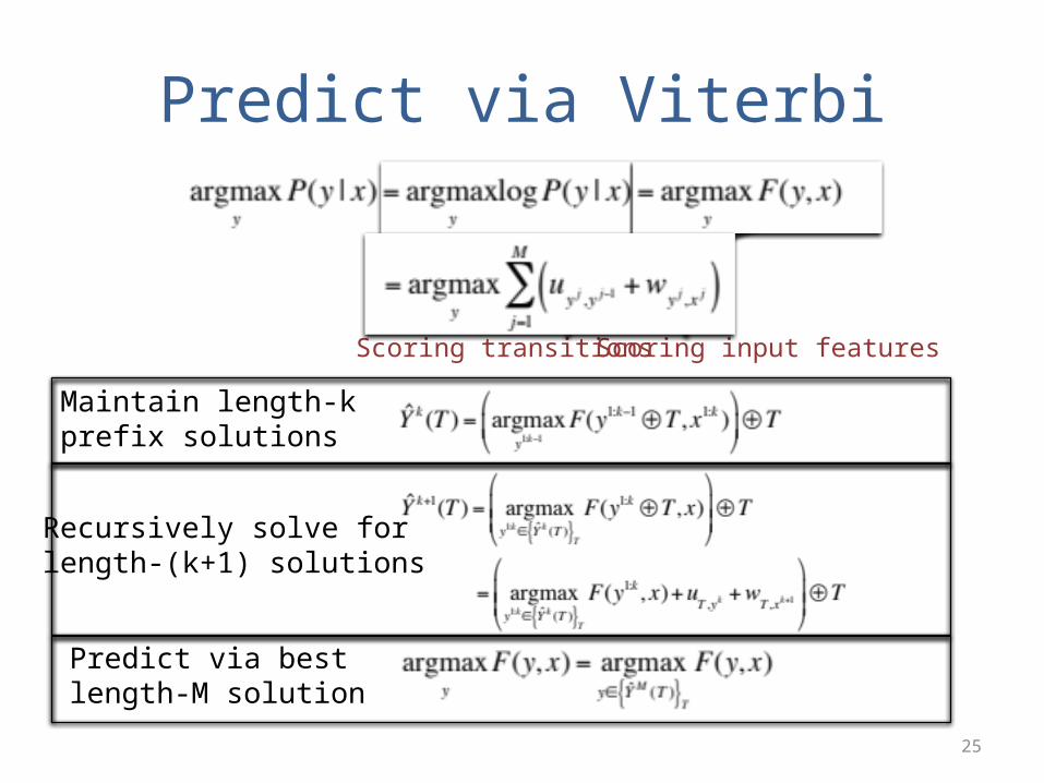
Predict via Viterbi

Scoring transitions Scoring input features

Maintain length-k prefix solutions

Recursively solve forlength-(k+1) solutions

Predict via bestlength-M solution

26

Ŷ1(V)

Ŷ1(D)

Ŷ1(N)

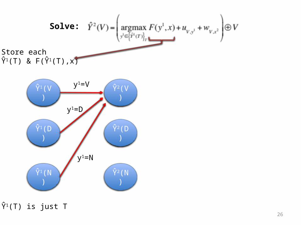
Store each Ŷ1(T) & F(Ŷ1(T),x)

Ŷ2(V)

Ŷ2(D)

Ŷ2(N)

Solve:

y1=V

y1=D

y1=N

Ŷ1(T) is just T

27

Ŷ1(V)

Ŷ1(D)

Ŷ1(N)

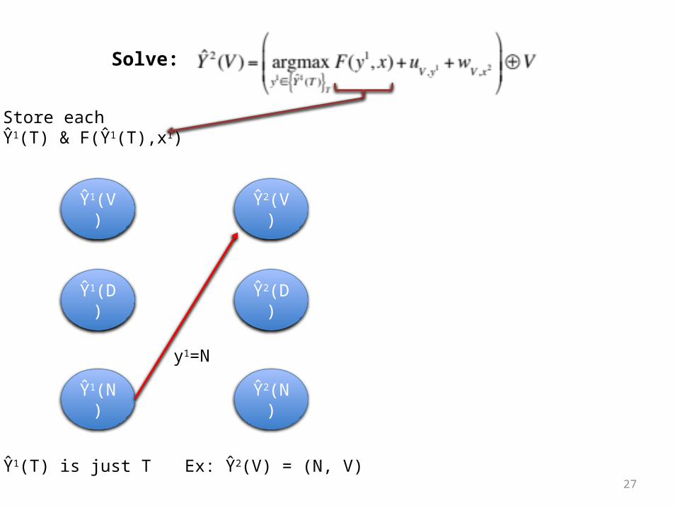
Store each Ŷ1(T) & F(Ŷ1(T),x1)

Ŷ2(V)

Ŷ2(D)

Ŷ2(N)

y1=N

Ŷ1(T) is just T Ex: Ŷ2(V) = (N, V)

Solve:

28

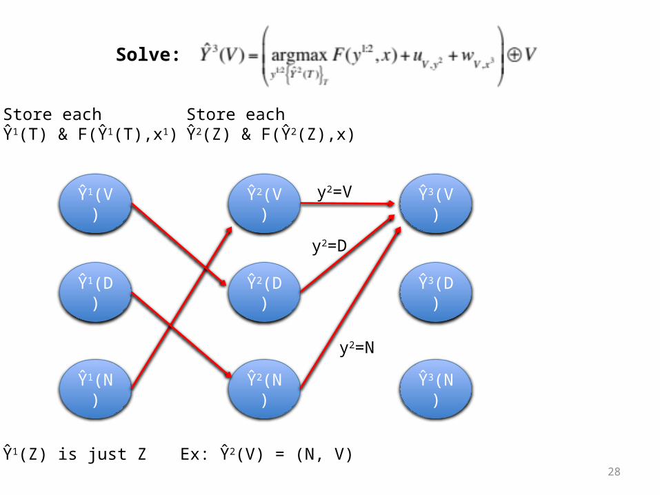
Ŷ1(V)

Ŷ1(D)

Ŷ1(N)

Store each Ŷ1(T) & F(Ŷ1(T),x1)

Ŷ2(V)

Ŷ2(D)

Ŷ2(N)

Store each Ŷ2(Z) & F(Ŷ2(Z),x)

Ex: Ŷ2(V) = (N, V)

Ŷ3(V)

Ŷ3(D)

Ŷ3(N)

Solve:

y2=V

y2=D

y2=N

Ŷ1(Z) is just Z

29

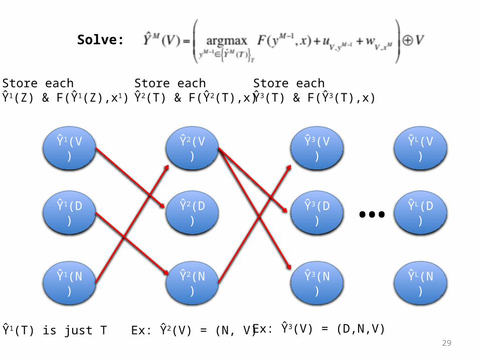
Ŷ1(V)

Ŷ1(D)

Ŷ1(N)

Store each Ŷ1(Z) & F(Ŷ1(Z),x1)

Ŷ2(V)

Ŷ2(D)

Ŷ2(N)


Ex: Ŷ2(V) = (N, V)

Ŷ3(V)

Ŷ3(D)

Ŷ3(N)


Ex: Ŷ3(V) = (D,N,V)

ŶL(V)

ŶL(D)

ŶL(N)

…

Ŷ1(T) is just T

Solve:

30

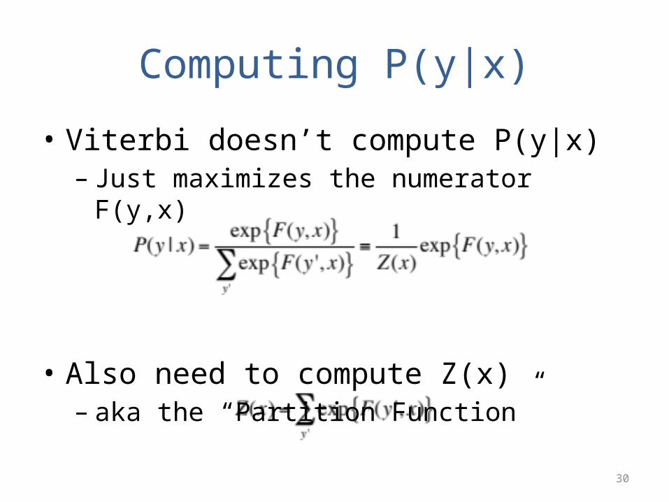
Computing P(y|x)

• Viterbi doesn’t compute P(y|x)– Just maximizes the numerator F(y,x)

• Also need to compute Z(x)– aka the “Partition Function”

31

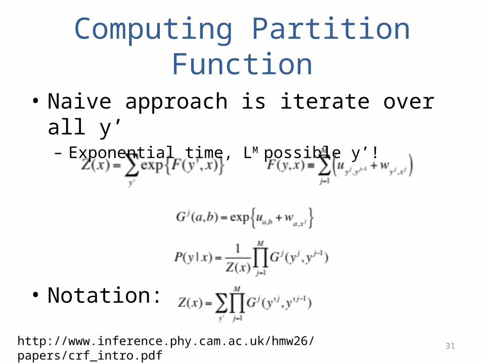
Computing Partition Function

• Naive approach is iterate over all y’– Exponential time, LM possible y’!

• Notation:

http://www.inference.phy.cam.ac.uk/hmw26/papers/crf_intro.pdf

32

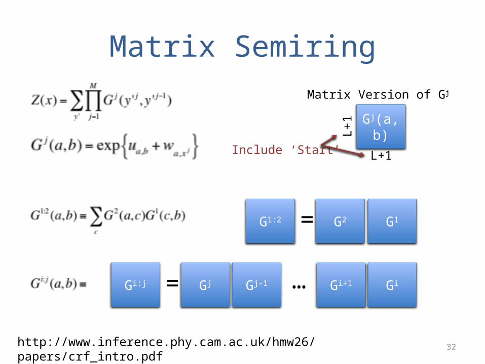
Matrix Semiring

Gj(a,b)

L+1

Matrix Version of Gj

G1:2 G2 G1=

Gi:j Gi+1 Gi= Gj Gj-1 …

L+1

Include ‘Start’


33

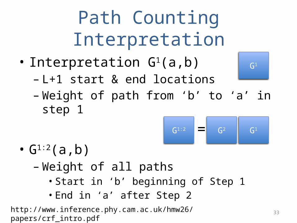
Path Counting Interpretation

• Interpretation G1(a,b) – L+1 start & end locations– Weight of path from ‘b’ to ‘a’ in step 1

• G1:2(a,b)– Weight of all paths• Start in ‘b’ beginning of Step 1• End in ‘a’ after Step 2

G1

G1:2 G2 G1=


34

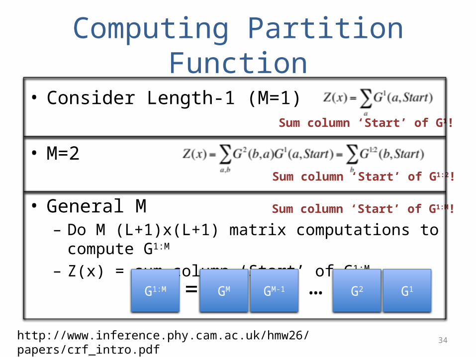
• Consider Length-1 (M=1)

• M=2

• General M– Do M (L+1)x(L+1) matrix computations to compute G1:M

– Z(x) = sum column ‘Start’ of G1:M

Computing Partition Function

Sum column ‘Start’ of G1!

Sum column ‘Start’ of G1:2!

G1:M G2 G1= GM GM-1 …

Sum column ‘Start’ of G1:M!


35

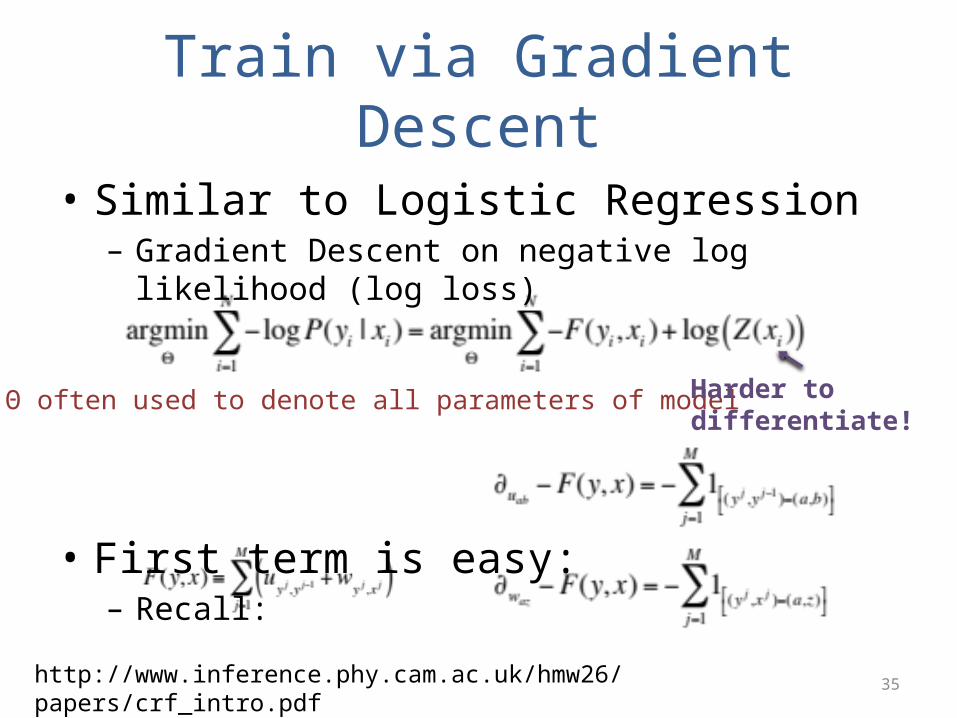
Train via Gradient Descent

• Similar to Logistic Regression– Gradient Descent on negative log likelihood (log loss)

• First term is easy:– Recall:

Θ often used to denote all parameters of model Harder todifferentiate!


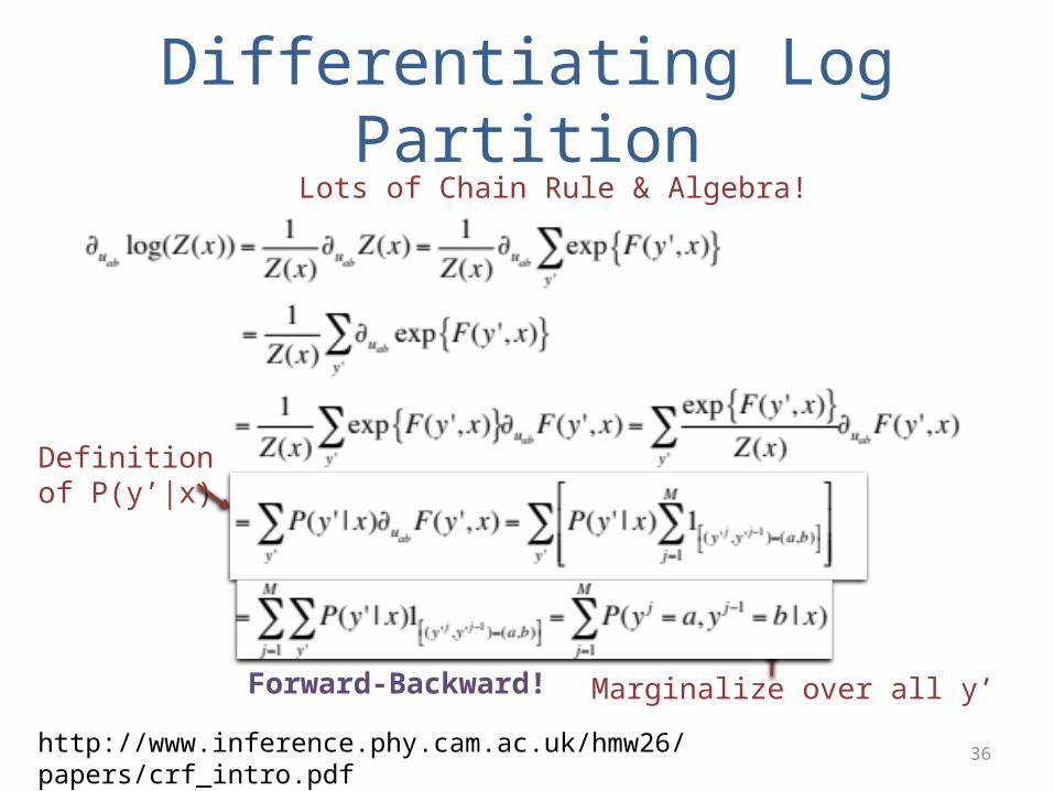
36

Differentiating Log PartitionLots of Chain Rule & Algebra!

Definition of P(y’|x)

Marginalize over all y’


Forward-Backward!

37

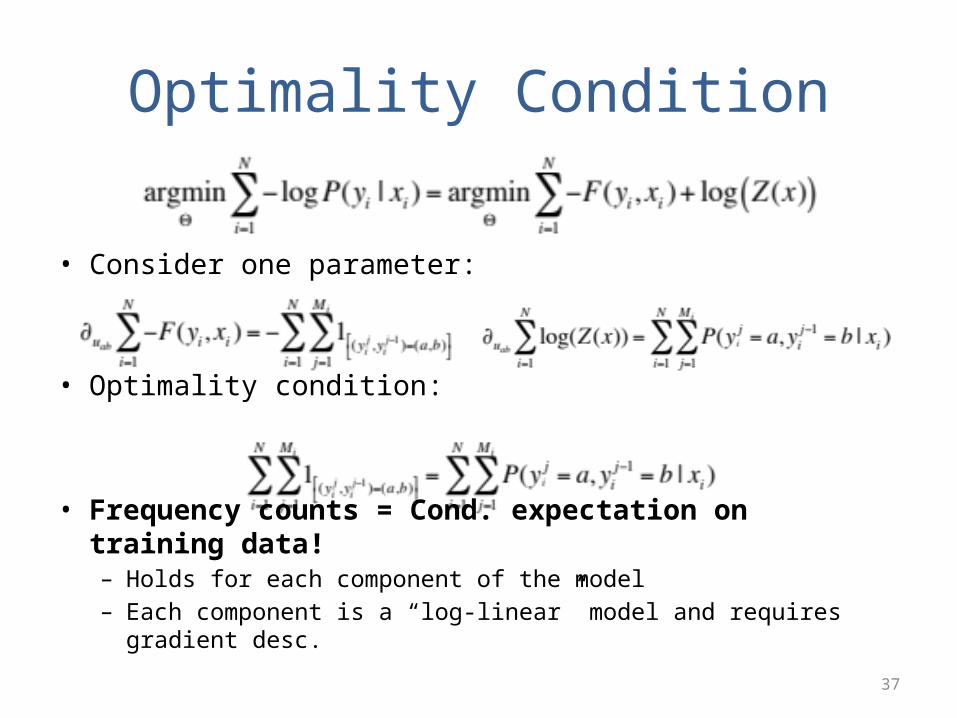
Optimality Condition

• Consider one parameter:

• Optimality condition:

• Frequency counts = Cond. expectation on training data!– Holds for each component of the model– Each component is a “log-linear” model and requires gradient desc.

38

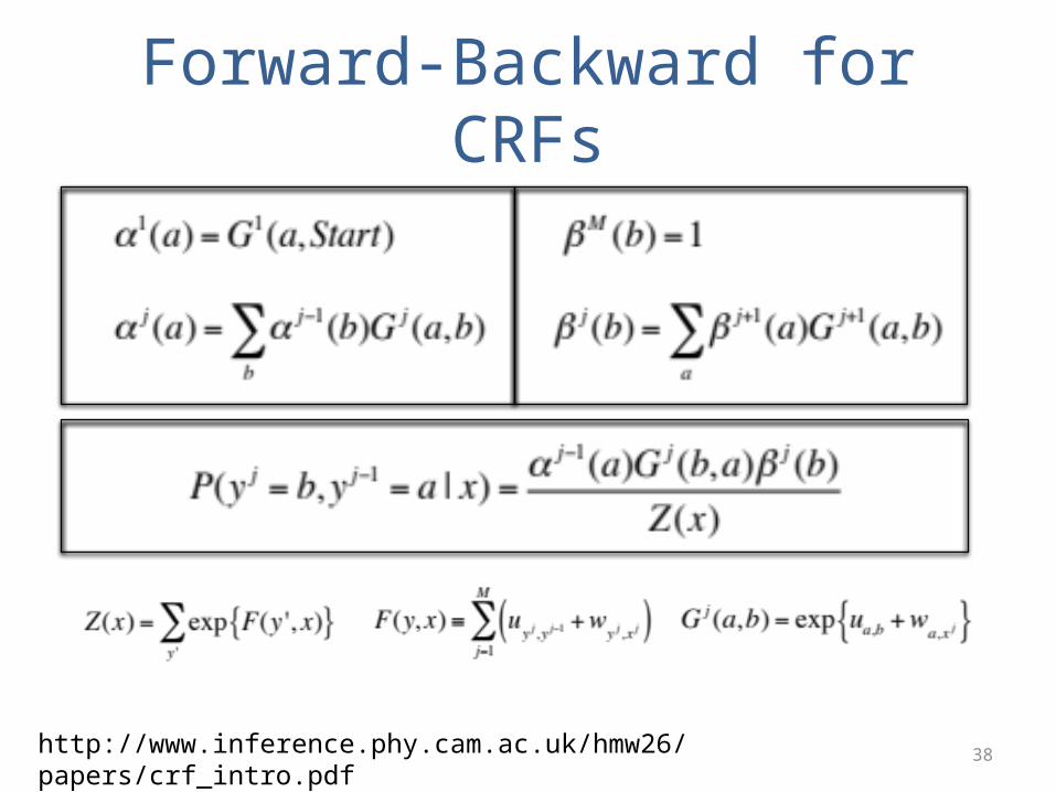
Forward-Backward for CRFs


39

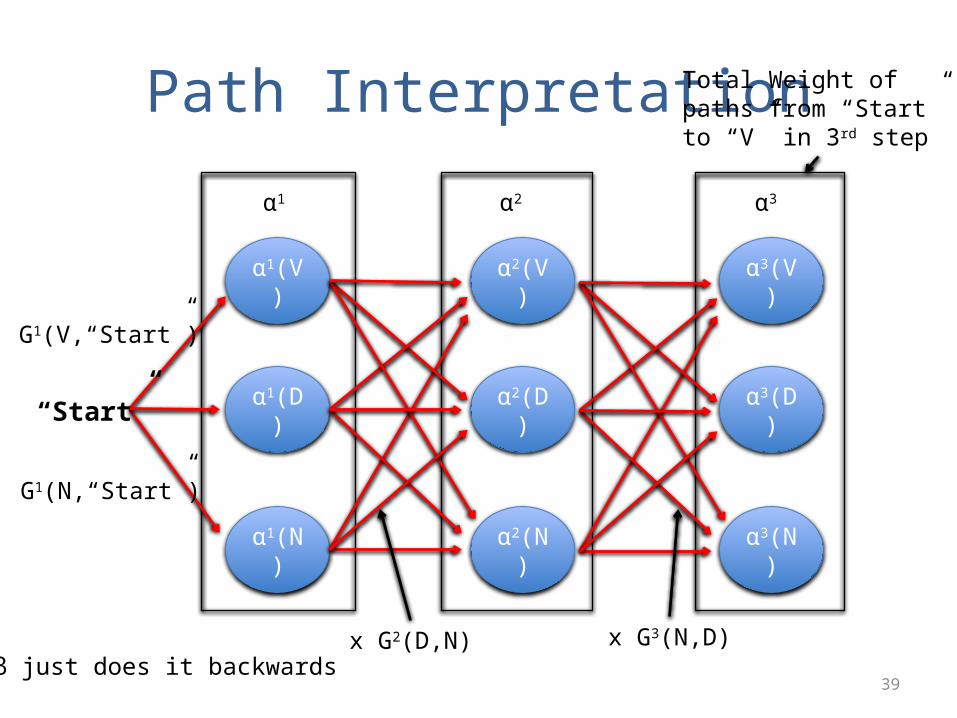
Path Interpretation

α1(V)

α1(D)

α1(N)

α2(V)

α2(D)

α2(N)

α3(V)

α3(D)

α3(N)

α1 α2 α3

“Start”

G1(V,“Start”)

G1(N,“Start”)

x G2(D,N) x G3(N,D)

Total Weight of paths from “Start” to “V” in 3rd step

β just does it backwards

40

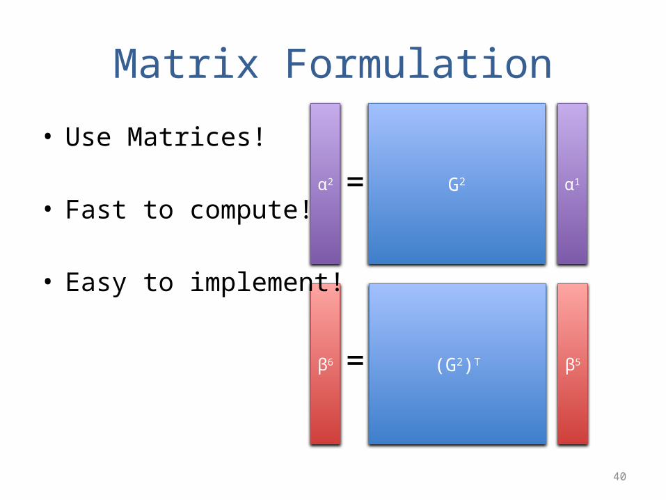
Matrix Formulation

G2 α1α2 =

(G2)T β5β6 =

• Use Matrices!

• Fast to compute!

• Easy to implement!

41

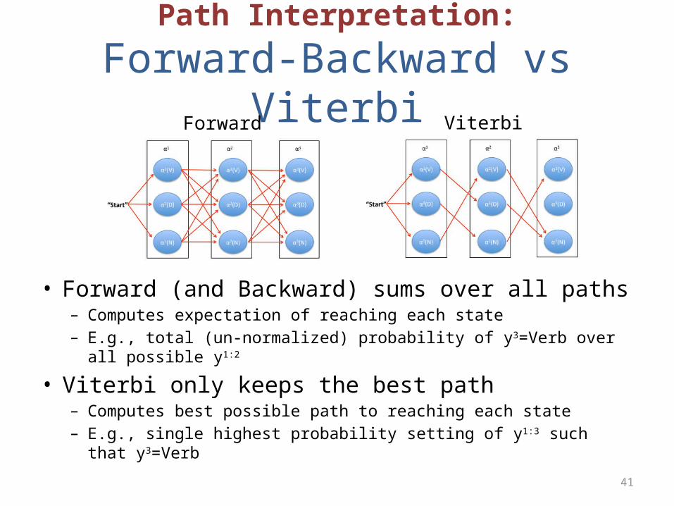
Path Interpretation:

Forward-Backward vs Viterbi

• Forward (and Backward) sums over all paths– Computes expectation of reaching each state– E.g., total (un-normalized) probability of y3=Verb over all possible y1:2

• Viterbi only keeps the best path– Computes best possible path to reaching each state– E.g., single highest probability setting of y1:3 such that y3=Verb

Forward Viterbi

42

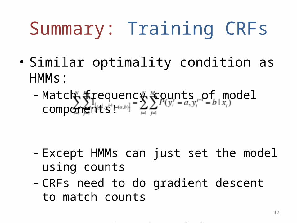
Summary: Training CRFs

• Similar optimality condition as HMMs:– Match frequency counts of model components!

– Except HMMs can just set the model using counts– CRFs need to do gradient descent to match counts

• Run Forward-Backward for expectation– Just like HMMs as well

43

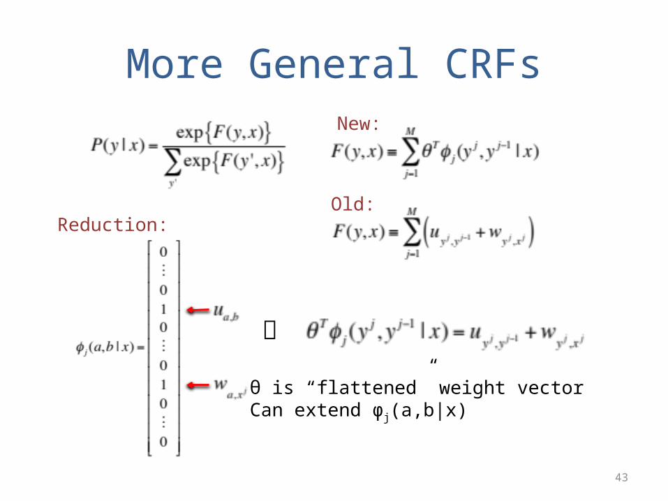
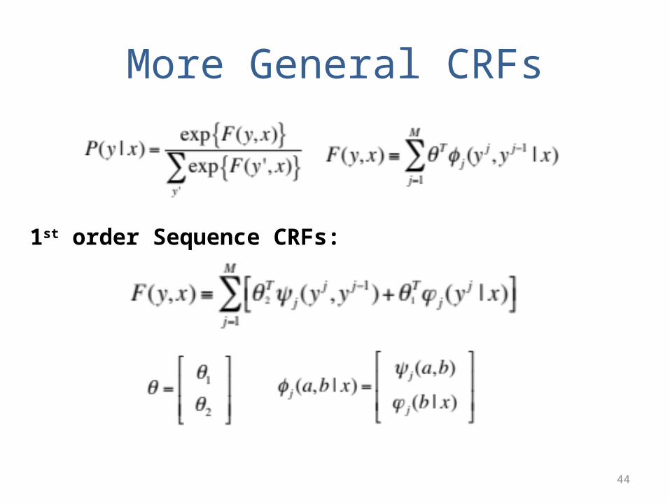
More General CRFsNew:

Old:Reduction:

θ is “flattened” weight vector Can extend φj(a,b|x)

44

More General CRFs

1st order Sequence CRFs:

45

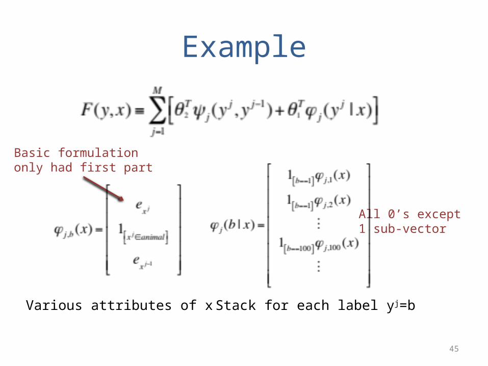
Example

Various attributes of x Stack for each label yj=b

All 0’s except 1 sub-vector

Basic formulation only had first part

46

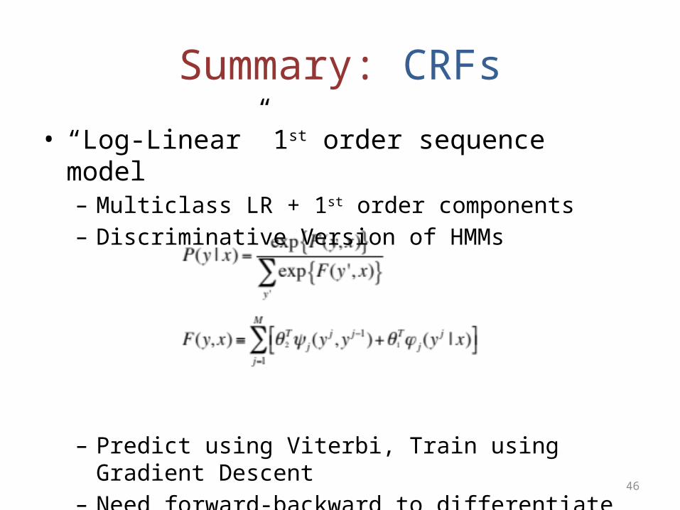
Summary: CRFs

• “Log-Linear” 1st order sequence model– Multiclass LR + 1st order components– Discriminative Version of HMMs

– Predict using Viterbi, Train using Gradient Descent– Need forward-backward to differentiate partition function

47

Next Week

• Structural SVMs– Hinge loss for sequence prediction

• More General Structured Prediction• Next Recitation: – Optimizing non-differentiable functions (Lasso)– Accelerated gradient descent

• Homework 2 due in 12 days– Tuesday, Feb 3rd at 2pm via Moodle

Documents

Machine Learning & Data Mining CS/CNS/EE 155 Lecture 6: Conditional Random Fields 1