MACHINE LEARNING FOR HEALTHCARE - GitHub Pages · MACHINE LEARNING FOR HEALTHCARE 6.S897, HST.S53 ... (Thanks to Peter Bodik for slides on reinforcement learning) Lecture 13: Finding

MACHINE LEARNING FOR HEALTHCARE6.S897, HST.S53

Prof. David SontagMIT EECS, CSAIL, IMES

(Thanks to Peter Bodik for slides on reinforcement learning)

Lecture 13: Finding optimal treatment policies

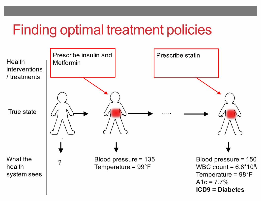
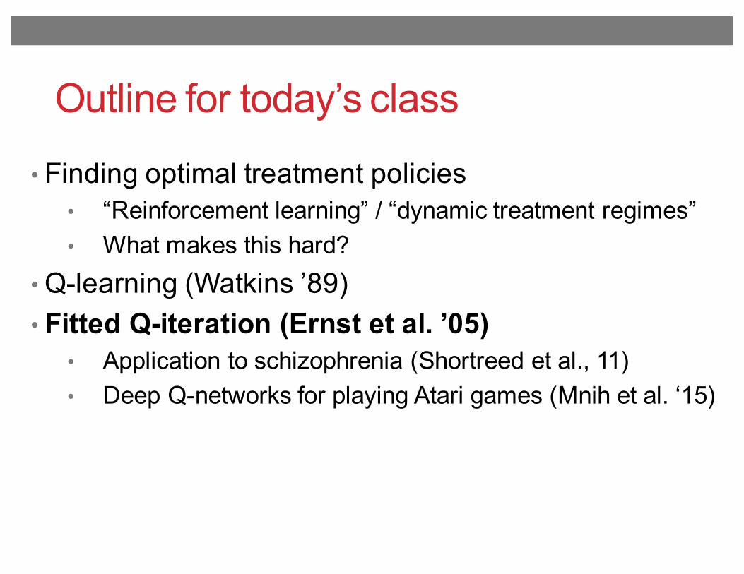
Outline for today’s class

• Finding optimal treatment policies• “Reinforcement learning” / “dynamic treatment regimes”• What makes this hard?

• Q-learning (Watkins ’89)• Fitted Q-iteration (Ernst et al. ’05)

• Application to schizophrenia (Shortreed et al., 11)• Deep Q-networks for playing Atari games (Mnih et al. ‘15)

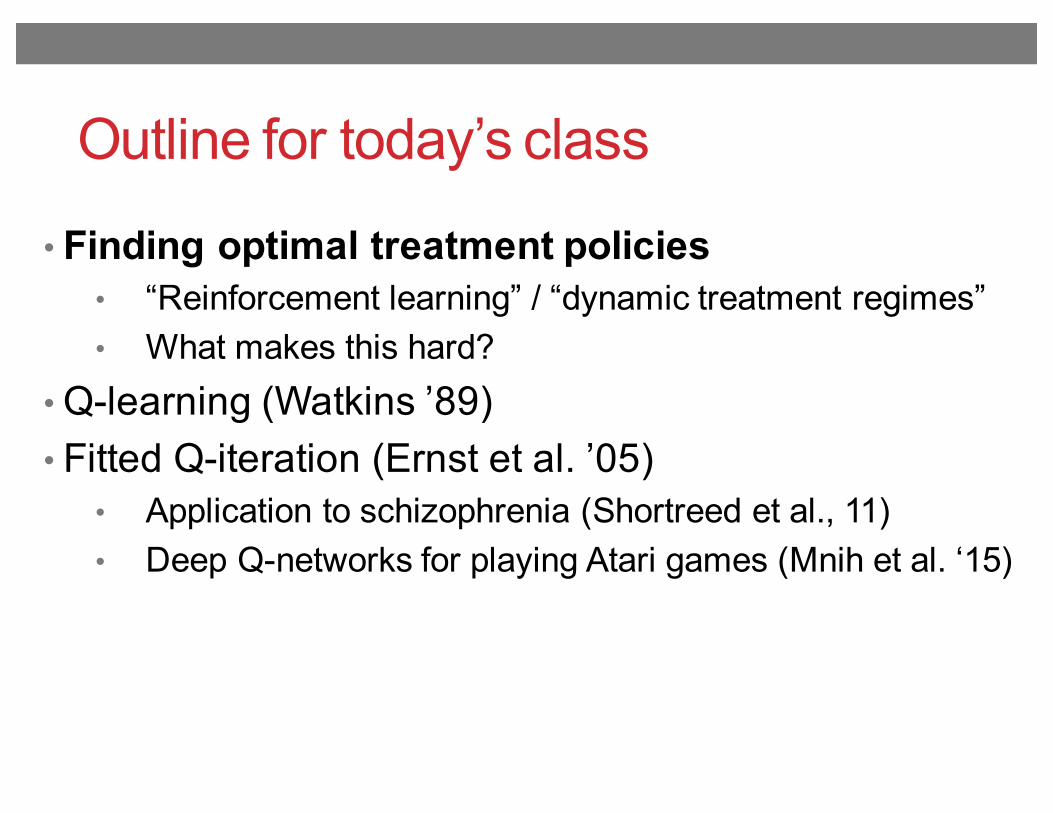
Previous Lectures• Supervised learning

• classification, regression

• Unsupervised learning• clustering

• Reinforcement learning• more general than supervised/unsupervised learning• learn from interaction w/ environment to achieve a goal

environment

agentactionreward

new state

[Slide from Peter Bodik]

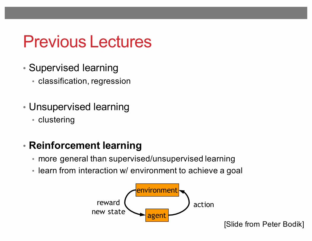
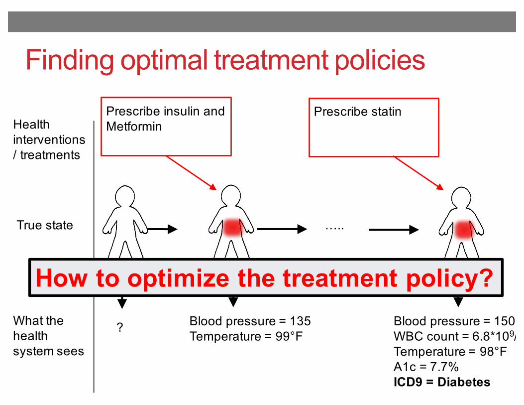
Finding optimal treatment policies

True state …..

What the health system sees

Blood pressure = 150WBC count = 6.8*109/LTemperature = 98°FA1c = 7.7%ICD9 = Diabetes

Blood pressure = 135Temperature = 99°F

?

Health interventions / treatments

Prescribe insulin and Metformin

Prescribe statin

Finding optimal treatment policies

True state …..

What the health system sees

Blood pressure = 150WBC count = 6.8*109/LTemperature = 98°FA1c = 7.7%ICD9 = Diabetes

Blood pressure = 135Temperature = 99°F

?

Health interventions / treatments

Prescribe insulin and Metformin

Prescribe statin

How to optimize the treatment policy?

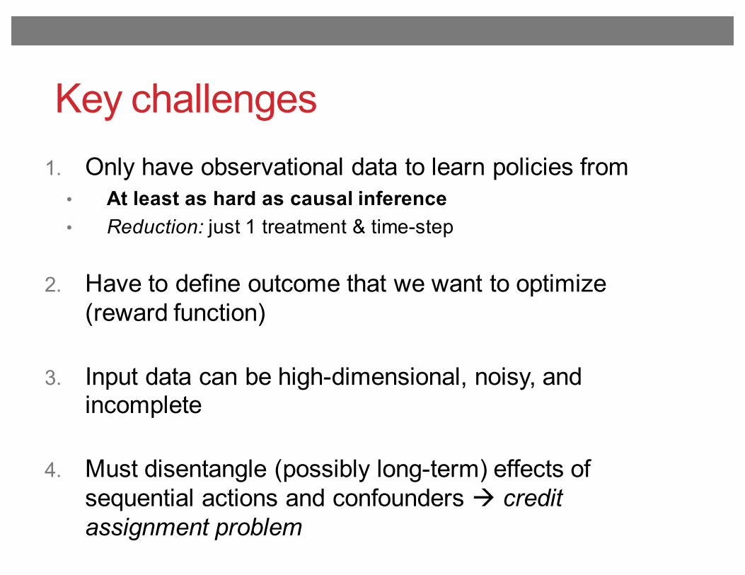
Key challenges1. Only have observational data to learn policies from

• At least as hard as causal inference• Reduction: just 1 treatment & time-step

2. Have to define outcome that we want to optimize (reward function)

3. Input data can be high-dimensional, noisy, and incomplete

4. Must disentangle (possibly long-term) effects of sequential actions and confounders à credit assignment problem

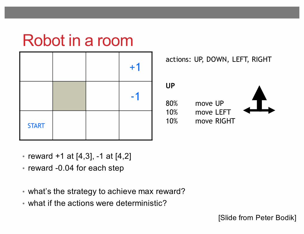
Robot in a room+1

-1

START

actions: UP, DOWN, LEFT, RIGHT

UP

80% move UP10% move LEFT10% move RIGHT

• reward +1 at [4,3], -1 at [4,2]• reward -0.04 for each step

• what’s the strategy to achieve max reward?• what if the actions were deterministic?


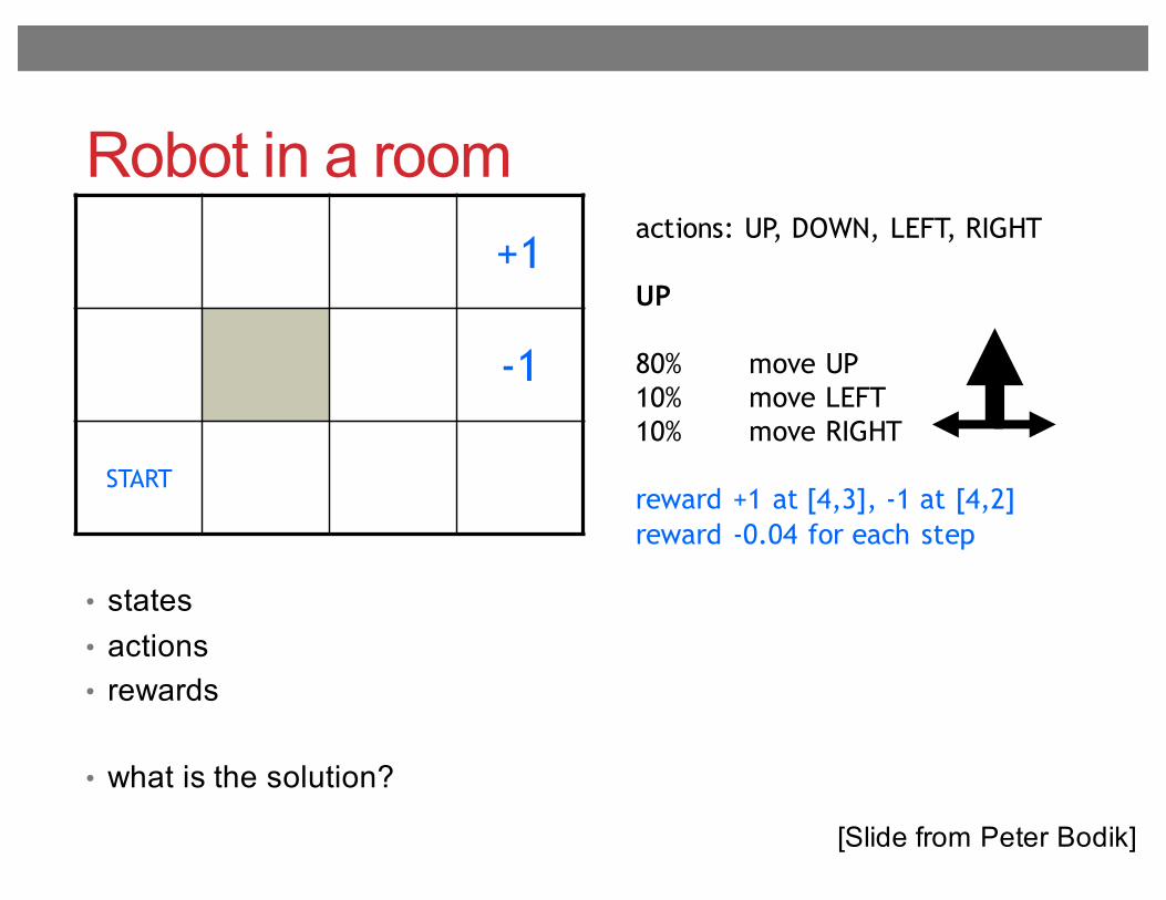
Robot in a room+1

-1

START

actions: UP, DOWN, LEFT, RIGHT

UP

80% move UP10% move LEFT10% move RIGHT

reward +1 at [4,3], -1 at [4,2]reward -0.04 for each step

• states• actions• rewards

• what is the solution?


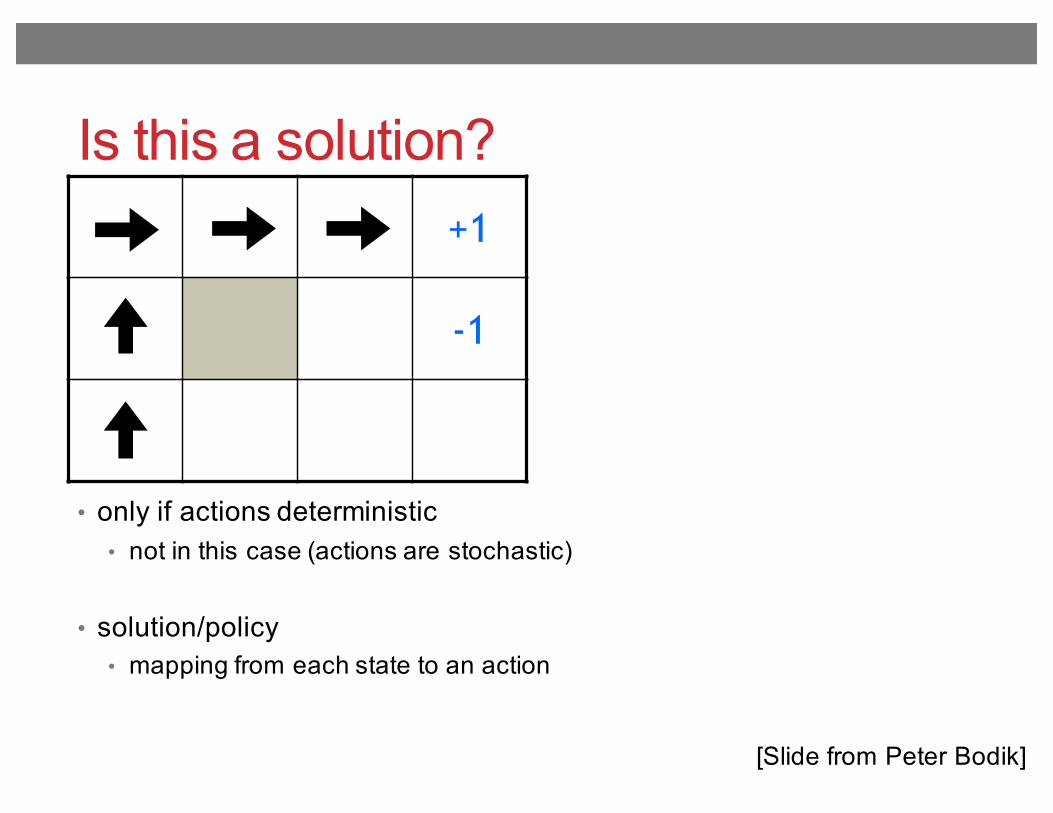
Is this a solution?+1

-1

• only if actions deterministic• not in this case (actions are stochastic)

• solution/policy• mapping from each state to an action


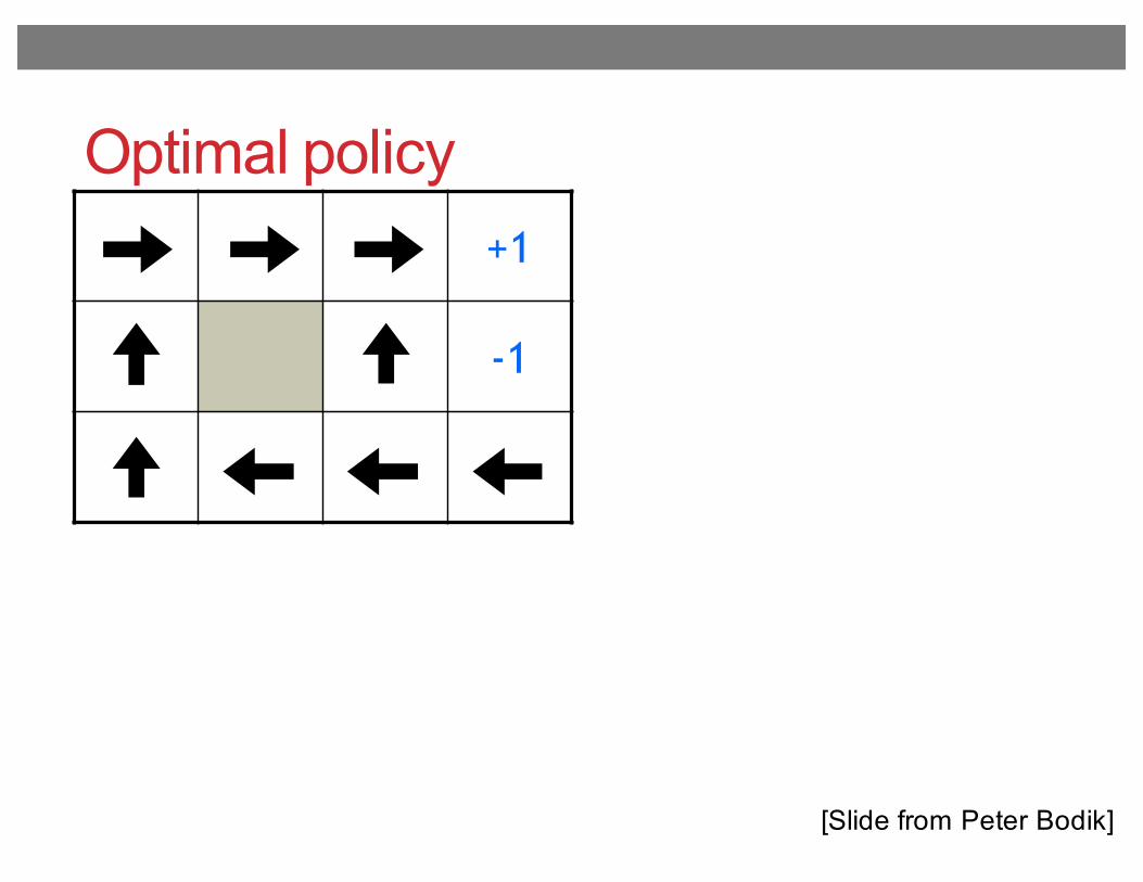
Optimal policy+1

-1


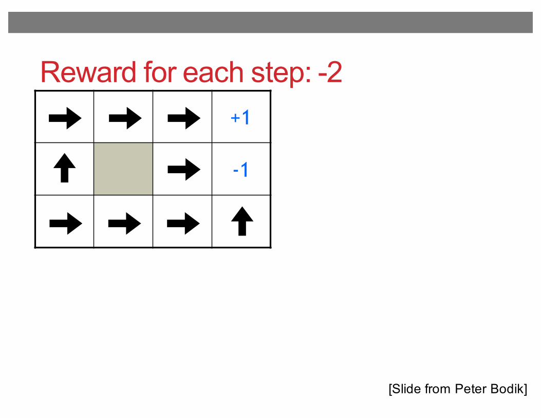
Reward for each step: -2+1

-1


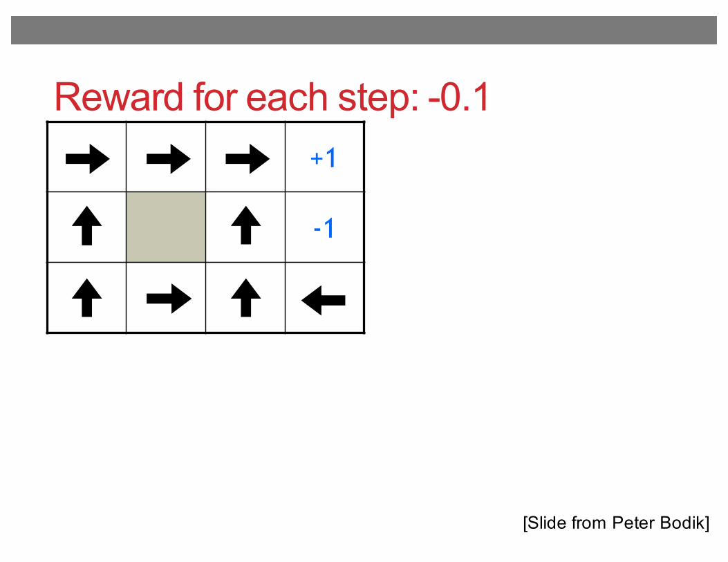
Reward for each step: -0.1+1

-1



-1



-1


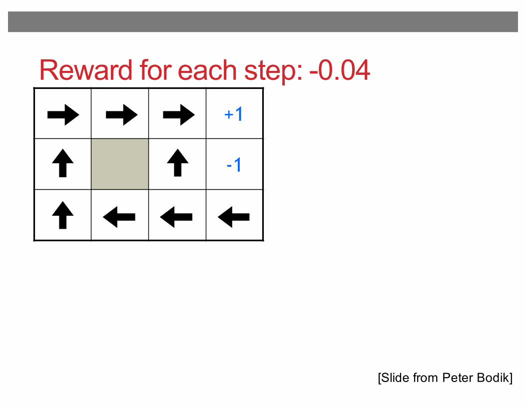
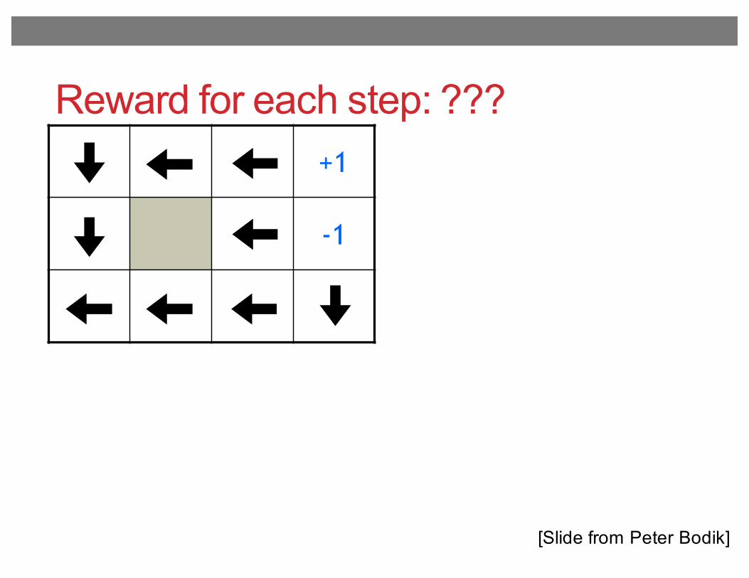
Reward for each step: ???+1

-1


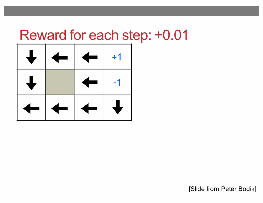
Reward for each step: +0.01+1

-1






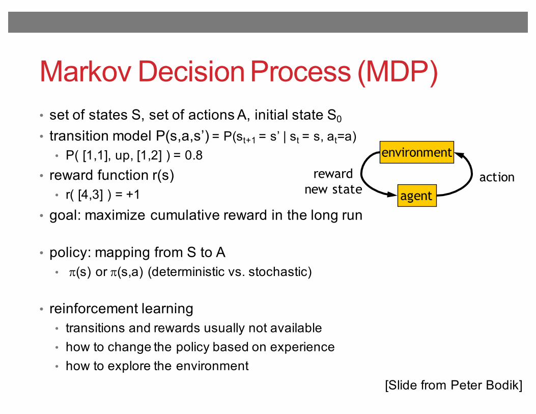
Markov Decision Process (MDP)• set of states S, set of actions A, initial state S0

• transition model P(s,a,s’) = P(st+1 = s’ | st = s, at=a)• P( [1,1], up, [1,2] ) = 0.8

• reward function r(s)• r( [4,3] ) = +1

• goal: maximize cumulative reward in the long run

• policy: mapping from S to A• p(s) or p(s,a) (deterministic vs. stochastic)

• reinforcement learning• transitions and rewards usually not available• how to change the policy based on experience• how to explore the environment

environment

agentactionreward

new state


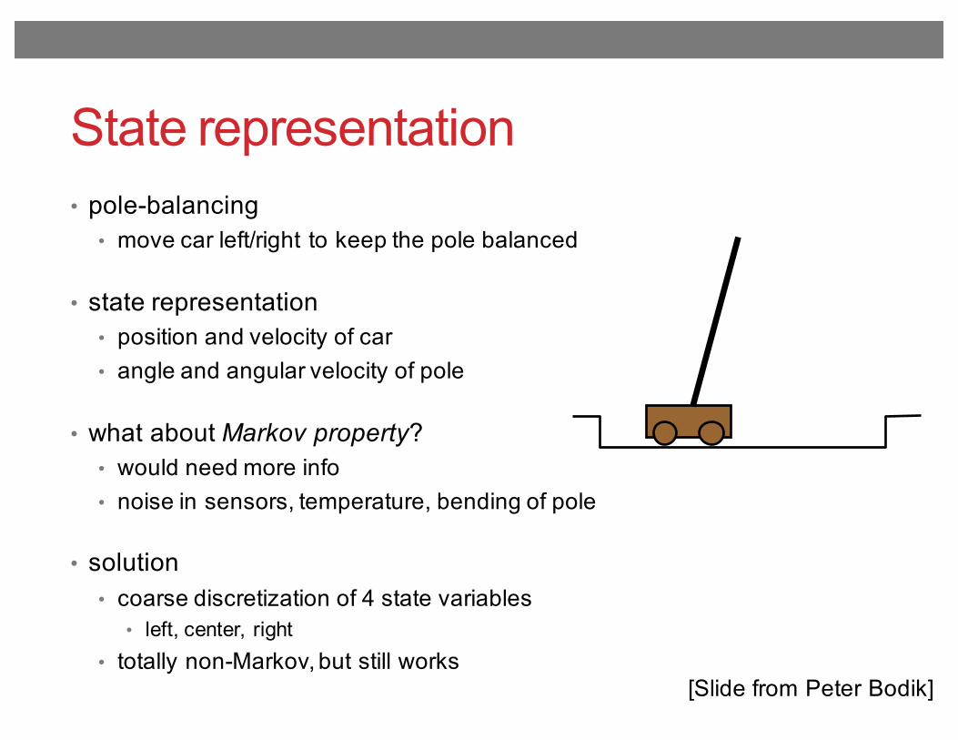
State representation• pole-balancing

• move car left/right to keep the pole balanced

• state representation• position and velocity of car• angle and angular velocity of pole

• what about Markov property? • would need more info• noise in sensors, temperature, bending of pole

• solution• coarse discretization of 4 state variables

• left, center, right• totally non-Markov, but still works


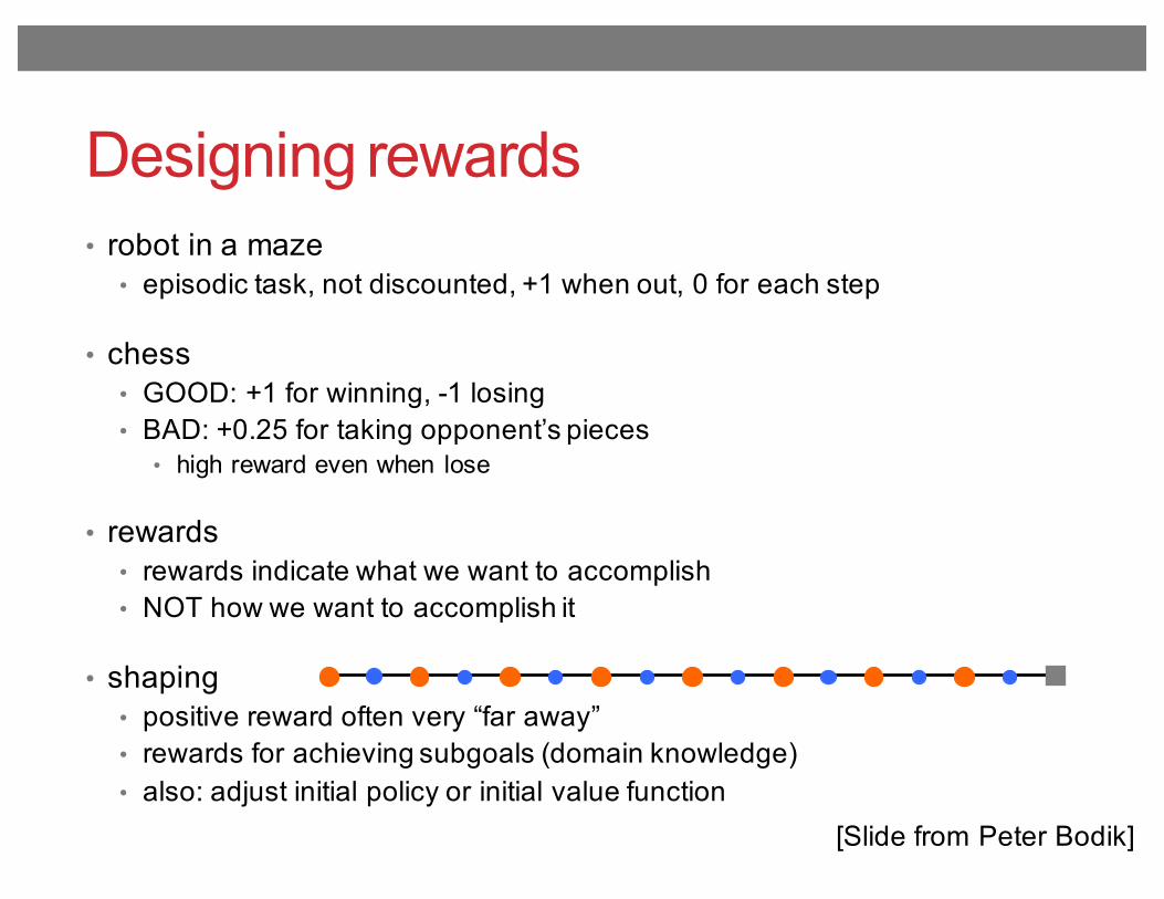
Designing rewards• robot in a maze

• episodic task, not discounted, +1 when out, 0 for each step

• chess• GOOD: +1 for winning, -1 losing• BAD: +0.25 for taking opponent’s pieces

• high reward even when lose

• rewards• rewards indicate what we want to accomplish• NOT how we want to accomplish it

• shaping• positive reward often very “far away”• rewards for achieving subgoals (domain knowledge)• also: adjust initial policy or initial value function


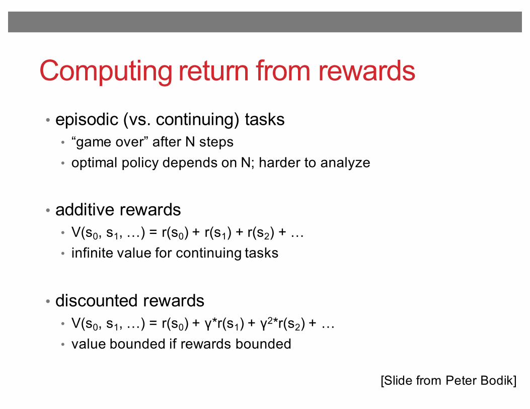
Computing return from rewards• episodic (vs. continuing) tasks

• “game over” after N steps• optimal policy depends on N; harder to analyze

• additive rewards• V(s0, s1, …) = r(s0) + r(s1) + r(s2) + …• infinite value for continuing tasks

• discounted rewards• V(s0, s1, …) = r(s0) + γ*r(s1) + γ2*r(s2) + …• value bounded if rewards bounded


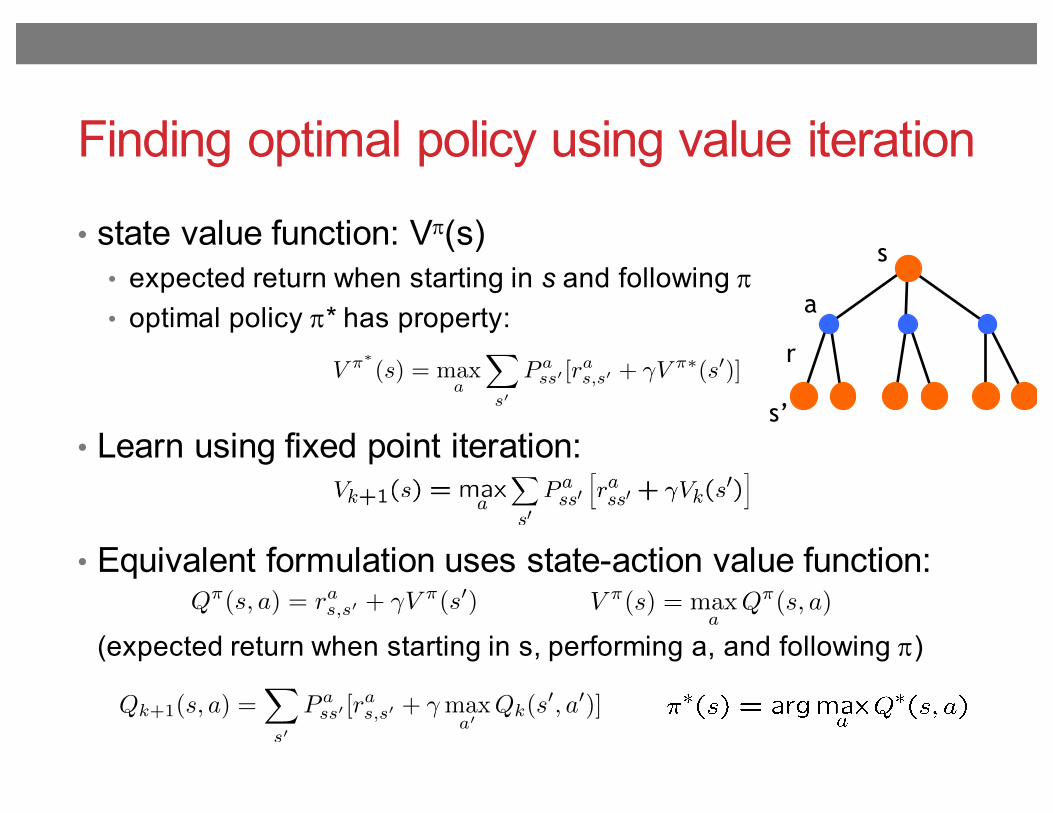
Finding optimal policy using value iteration

• state value function: Vp(s)• expected return when starting in s and following p• optimal policy p* has property:

• Learn using fixed point iteration:

• Equivalent formulation uses state-action value function:

(expected return when starting in s, performing a, and following p)

s

a

s’

r

V ⇡(s) = max

aQ⇡

(s, a)Q⇡(s, a) = ras,s0 + �V ⇡(s0)

V ⇡⇤(s) = max

a

X

s0

P ass0 [r

as,s0 + �V ⇡⇤

(s0)]

Qk+1(s, a) =X

s0

P ass0 [r

as,s0 + �max

a0Qk(s

0, a0)]

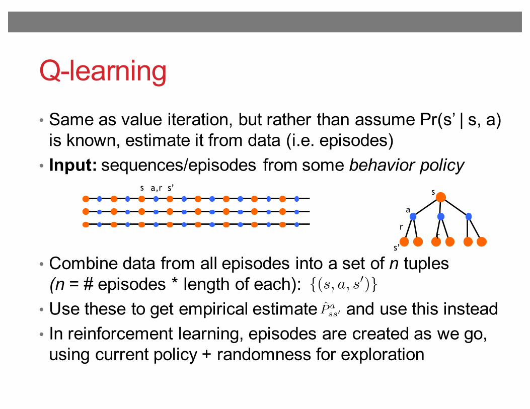
Q-learning• Same as value iteration, but rather than assume Pr(s’ | s, a)

is known, estimate it from data (i.e. episodes)• Input: sequences/episodes from some behavior policy

• Combine data from all episodes into a set of n tuples(n = # episodes * length of each):

• Use these to get empirical estimate and use this instead• In reinforcement learning, episodes are created as we go,

using current policy + randomness for exploration

s

a

s’

r

s a,r

r

s’

{(s, a, s0)}P̂ ass0

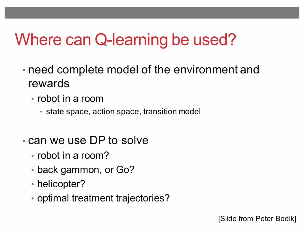
Where can Q-learning be used?

• need complete model of the environment and rewards• robot in a room

• state space, action space, transition model

• can we use DP to solve• robot in a room?• back gammon, or Go?• helicopter?• optimal treatment trajectories?






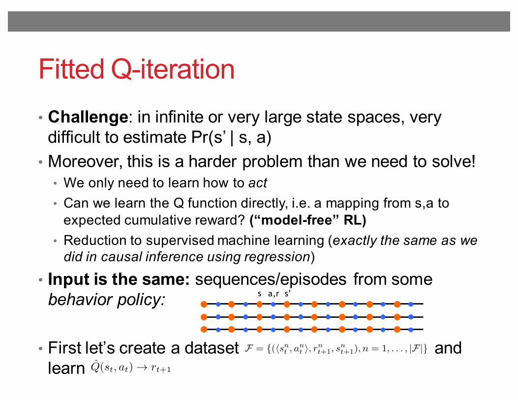
Fitted Q-iteration• Challenge: in infinite or very large state spaces, very

difficult to estimate Pr(s’ | s, a) • Moreover, this is a harder problem than we need to solve!

• We only need to learn how to act• Can we learn the Q function directly, i.e. a mapping from s,a to

expected cumulative reward? (“model-free” RL)• Reduction to supervised machine learning (exactly the same as we

did in causal inference using regression)

• Input is the same: sequences/episodes from some behavior policy:

• First let’s create a dataset and learn

s a,r s’

F = {(hsnt , ant i, rnt+1, snt+1), n = 1, . . . , |F|}

Q̂(st, at) ! rt+1

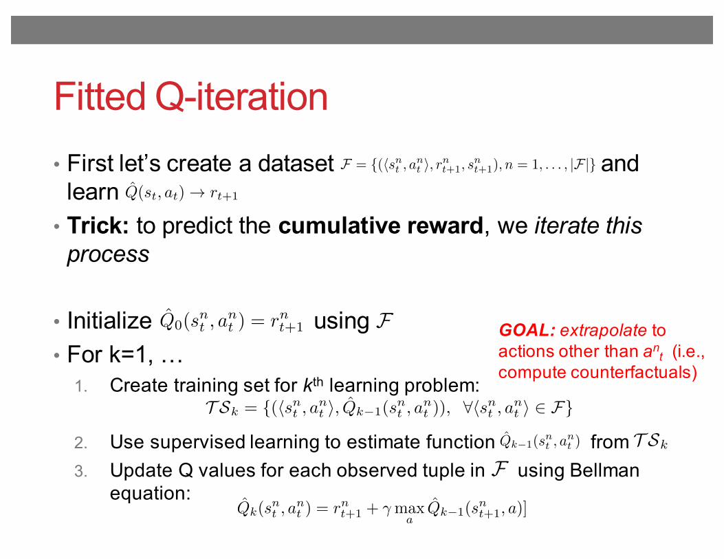
Fitted Q-iteration• First let’s create a dataset and

learn• Trick: to predict the cumulative reward, we iterate this

process

• Initialize using • For k=1, …

1. Create training set for kth learning problem:

2. Use supervised learning to estimate function from 3. Update Q values for each observed tuple in using Bellman

equation:

T Sk

GOAL: extrapolate to actions other than an

t (i.e., compute counterfactuals)

F

ˆQk(snt , a

nt ) = rnt+1 + �max

aˆQk�1(s

nt+1, a)]

F = {(hsnt , ant i, rnt+1, snt+1), n = 1, . . . , |F|}

Q̂(st, at) ! rt+1

Q̂0(snt , a

nt ) = rnt+1

T Sk = {(hsnt , ant i, Q̂k�1(snt , a

nt )), 8hsnt , ant i 2 F}

Q̂k�1(snt , a

nt )

F

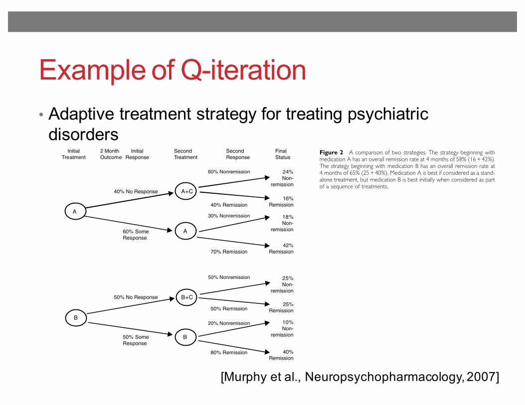
Example of Q-iteration• Adaptive treatment strategy for treating psychiatric

disorders

[Murphy et al., Neuropsychopharmacology, 2007]

demonstrate the utility of these designs and to illuminateany unexpected issues.

Constructing Decision Rules from Data

Why are new ways of analyzing data needed? It turns outthat in many cases the construction of optimized treatmentdecision rules requires a more holistic approach thanexpected. For example, it is tempting to ascertain the besttreatment at any given time ignoring future treatments. Thisapproach, however, can lead to erroneous conclusionsabout the best sequence of treatments. The effect of thesequence cannot be accurately estimated by evaluating onlya single treatment episode. For example, an initial course ofcognitive therapy for depression may be much moreeffective in the long term when followed by less frequenttherapy sessions (continuation treatment) than whenfollowed by waiting without therapy (Jarrett et al, 1998).Consider two treatments (A and B) that differ in terms of

immediate response, favoring A. But when B is followed byB augmented with C, the longer-term response during theentire time period may exceed the effect of A followed byA augmented with C (Figure 2). This occurs for two reasons.First, if a patient responds to B then the patient is morelikely to either remain in or progress to remission asopposed to a patient who responds to A. Second, treatmentB followed by B+C is synergistic, that is among those whodo not respond to B, treatment B +C produces higherremission rate as compared to the effect of treatment A+Camong those who did not respond initially to A.Similarly a treatment may be very useful in the long term,

but may entail greater cost or inconvenience in the shortterm. For instance, cognitive therapy may be useful in

reducing relapses, once the treatment is stopped (Fava et al,1998, 2001; Hollon et al, 2005) yet it is more timeconsuming and expensive in the short term. So, too, vagusnerve stimulation (Rush et al, 2005a, b; Sackeim et al, 2001;George et al, 2005) may have only modest or minimal short-term effects, yet in the longer-term, efficacy may increase.The fact that one should incorporate the effects of futuretreatment decisions when evaluating present treatment iswell known to scientists who work on improving sequentialdecision making (Parmigiani, 2002; see comments onmyopic decisions in Sutton and Barto (1998)). There aremethods for constructing decision rules that incorporate theeffects of future decisions when evaluating present treat-ment decisions (Thall et al, 2000; Pineau et al, 2003;Parmigiani, 2002; Qin and Badgwell, 2003; Braun et al, 2001;Sutton and Barto, 1998; Murphy et al, 2001; Murphy, 2003;Robins, 2004). These methods also permit the evaluation ofthe tailoring variables.One intuitive computer science technique for construct-

ing decision rules is called ‘Q-learning’ (Sutton and Barto,1998; Blatt et al, 2004). Q-learning explicitly incorporatesthe effects of future decisions; it is a generalization of thefamiliar regression model. To illustrate a simple version ofQ-Learning suppose the goal is to minimize the averagelevel of depression over a 4-month period, and suppose thatdata from the SMART design in Figure 1 is available. Notethere are only two key decisions in this rather simple trial,the initial treatment decision and then the second treatmentdecision (for those not responding satisfactorily to theinitial treatment). Suppose further that remission and side-effect level are to be used as tailoring variables in decisionmaking.In Q-learning with SMART data the construction of the

decision rules works backwards from the last decision to thefirst decision. As there are two treatment decisions there aretwo regressions. Consider the last (here second) treatmentdecision. This regression uses data from subjects whosedepression did not remit by 8 weeks. A simple model uses asummary of depression during weeks 9 through 12 as theindependent variable (Y2) and the regression model

b0 þ b1S8 þ ðb2 þ b3S8ÞT2 ð1ÞThe subscript 8 indicates that the side-effect level, S8, is asummary of side effects up to the end of the eighth week. Ingeneral the regression might include further potentialtailoring variables such as number of past depressionepisodes, adherence level during initial 8 weeks and theinitial treatment to which the subject was assigned. Thetreatment T2 is coded as 1 if the switch is assigned andis coded as 0 if augmentation is assigned. In this simplecase, the decision rule recommends a switch in treatmentfor a patient with nonremitting depression if b0 + b1S8 +(b2 + b3S8) is smaller than b0 + b1S8 and recommends anaugmentation otherwise (ie, recommend a switch if b2 +b3S8o0). If one expects that the higher the side effects S8are, the better it is to switch treatment, then b3 will benegative.Now consider the initial decision. In this regression we

use data from all subjects regardless of whether theirdepression remitted. It is insufficient to use a summary ofdepression during the first 8 weeks (Y1) or the indicator ofremission as the independent variable because both of these

InitialTreatment

2 MonthOutcome

InitialResponse

SecondTreatment

SecondResponse

FinalStatus

60% Nonremission

30% Nonremission

50% Nonremission

20% Nonremission

24%Non-

remission

18%Non-

remission

40% No Response A+C16%

Remission

42%Remission

10%Non-

remission

40%Remission

25%Non-

remission

25%Remission

40% Remission

70% Remission

50% Remission

80% Remission

A

60% SomeResponse

50% No Response

50% SomeResponse

A

B+C

B

B

Figure 2 A comparison of two strategies. The strategy beginning withmedication A has an overall remission rate at 4 months of 58% (16 + 42%).The strategy beginning with medication B has an overall remission rate at4 months of 65% (25+ 40%). Medication A is best if considered as a stand-alone treatment, but medication B is best initially when considered as partof a sequence of treatments.

Treatment sequences for chronic psychiatric disordersSA Murphy et al

260

Neuropsychopharmacology











InitialTreatment

2 MonthOutcome

InitialResponse

SecondTreatment

SecondResponse

FinalStatus

60% Nonremission

30% Nonremission

50% Nonremission

20% Nonremission

24%Non-

remission

18%Non-

remission


Remission

42%Remission

10%Non-

remission

40%Remission

25%Non-

remission

25%Remission

40% Remission

70% Remission

50% Remission

80% Remission

A

60% SomeResponse

50% No Response

50% SomeResponse

A

B+C

B

B



260


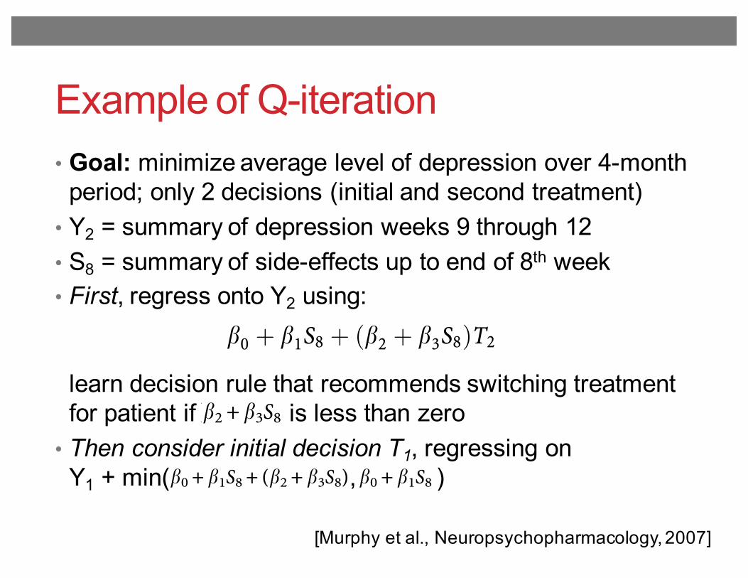
Example of Q-iteration• Goal: minimize average level of depression over 4-month

period; only 2 decisions (initial and second treatment)• Y2 = summary of depression weeks 9 through 12• S8 = summary of side-effects up to end of 8th week• First, regress onto Y2 using:

learn decision rule that recommends switching treatment for patient if is less than zero

• Then consider initial decision T1, regressing onY1 + min( , )

[Murphy et al., Neuropsychopharmacology, 2007]











InitialTreatment

2 MonthOutcome

InitialResponse

SecondTreatment

SecondResponse

FinalStatus

60% Nonremission

30% Nonremission

50% Nonremission

20% Nonremission

24%Non-

remission

18%Non-

remission


Remission

42%Remission

10%Non-

remission

40%Remission

25%Non-

remission

25%Remission

40% Remission

70% Remission

50% Remission

80% Remission

A

60% SomeResponse

50% No Response

50% SomeResponse

A

B+C

B

B



260












InitialTreatment

2 MonthOutcome

InitialResponse

SecondTreatment

SecondResponse

FinalStatus

60% Nonremission

30% Nonremission

50% Nonremission

20% Nonremission

24%Non-

remission

18%Non-

remission


Remission

42%Remission

10%Non-

remission

40%Remission

25%Non-

remission

25%Remission

40% Remission

70% Remission

50% Remission

80% Remission

A

60% SomeResponse

50% No Response

50% SomeResponse

A

B+C

B

B



260


represent only short-term benefits instead of both short-and long-term benefits of the initial treatment. Instead aterm is added to Y1; this term represents longer-termbenefits of the initial decision. Denote this additional termby V; model (1) provides V for the nonremitting subjects. Inthis case, V is the smaller of b0 + b1S8 + (b2 + b3S8) and b0 +b1S8. The former term is smaller if a switch in treatment wasfound to be best. V represents the effect of the initialdecision on both the depression summary during weeks9–16 and on the best second treatment decision (if subject’sdepression did not remit by week 8). If a subject’sdepression remitted by week 8 then V is simply thepredicted Y2 from a regression of Y2 on S8 for the remittingsubjects. The regression for the initial treatment decisionuses Y1 +V as the independent variable and the regressionmodel: a0 + a1T1 where treatment T1 is coded as 1 if themedication A is assigned and is coded as 0 otherwise. In thissimple case, the decision rule recommends medication A ifa1 is positive and recommends medication B otherwise. Ingeneral one would include dependent variables such asnumber of past depression episodes and other subjectcharacteristics.

Needed research and collaboration. Although there areseveral methods for using data to construct adaptivetreatment strategies, these methods have not been evaluatedin realistic settings. Collaborations are needed to providepractical evaluations of existing methods, like Q-Learning,for developing adaptive treatment strategies. For example,the illustration provided above is somewhat simplistic. Inpractice, there are often more than two decisions, each mayinvolve a choice between more than two options, theregression models might not be linear, and there may be avariety of outcomes.

DISCUSSION

Effective management of chronic psychiatric disorderspresents many challenges. Response heterogeneity iscommon, treatments may become burdensome, adherenceis problematic, and many patients may relapse. Additionallythese disorders often occur in conjunction with other healthand social problems. These disorder characteristics and thetreatment/social settings in which they occur motivate thedevelopment of adaptive treatment strategies. Addressingtactical questions concerning the length of time to wait fortreatment response and the choice of subsequent treatmentare crucial in this endeavor. We have discussed a variety ofpromising methodologies in developing adaptive treatmentstrategies. These methodologies, however, while clearlyuseful in other scientific domains, are relatively untestedin the fields of psychiatric disorders. Thus, the primarychallenge is to form collaborative teams to evaluate theseand other methodologies to construct evidence-basedadaptive treatment strategies. These interdisciplinary,collaborative, teams can spur new ways to conceptualizesequential decision making and enable the use of newmethodologies in improving clinical care for individualswith chronic disorders. The scientific opportunities, poten-tial for improved patient care, and the intellectualchallenges entailed in such work provide strong incentivesfor such efforts.

ACKNOWLEDGEMENTS

The MCATS network is funded by NIH Roadmap-AffiliatedGrant: 1R21 DA019800. National Institute on Drug AbuseGrants K02-DA15674 and P50 DA10075 supported thisproject.

REFERENCES

Adli M, Bauer M, Rush AJ (2006). Algorithms and collaborativecare systems for depression: are they effective and why? Asystematic review. Biol Psychiatry 59: 1029–1038.

American Psychiatric Association (2000). Practice guideline fortreatment of patients with major depressive disorder (revision).Am J Psychiatry 157: 1–45.

Blatt D, Murphy SA, Zhu J (2004). A-learning for approximateplanning. Technical Report 04-63, The Methodology Center.Pennsylvania State University.

Braun MW, Rivera DE, Stenman A (2001). A model-on-demandidentification methodology for nonlinear process systems. Int JControl 74: 1708–1717.

Collins LM, Murphy SA, Bierman KL (2004). A conceptualframework for adaptive preventive interventions. Prev Sci 5:185–196.

Crismon ML, Trivedi M, Pigott TA, Rush AJ, Hirschfeld RM, KahnDA et al (1999). The Texas medication algorithm project: reportof the Texas consensus conference panel on medicationtreatment of major depressive disorder. J Clin Psychiatry 60:142–156.

Dawson R, Lavori PW (2004). Placebo-free designs for evaluatingnew mental health treatments: the use of adaptive treatmentstrategies. Stat Med 23: 3249–3262.

Fava GA, Bartolucci G, Rafanelli C, Mangelli L (2001). Cognitive-behavioral management of patients with bipolar disorderwho relapsed while on lithium prophylaxis. J Clin Psychiatry62: 556–559.

Fava GA, Rafanelli C, Grandi S, Conti S, Belluardo P (1998).Prevention of recurrent depression with cognitive behavioraltherapy: preliminary findings. Arch Gen Psychiatry 55: 816–820.

Fava M, Rush AJ, Trivedi MH, Nierenberg AA, Thase ME, SackeimHA et al (2003). Background and rationale for the sequencedtreatment alternatives to relieve depression. (STAR*D) study.Psychiatr Clin North Am 26: 457–494.

George MS, Rush AJ, Marangell LB, Sackeim HA, Brannan SK,Davis SM et al (2005). A one-year comparison of vagus nervestimulation with treatment as usual for treatment-resistantdepression. Biol Psychiatry 58: 364–373.

Hirschfeld RM (2003). Long-term side effects of SSRIs: sexualdysfunction and weight gain. J Clin Psychiatry 18(Suppl 64):20–24.

Hollon SD, Beck AT (2004). Cognitive and cognitive behavioraltherapies. In: Lambert MJ (ed). Garfield and Bergin’s Handbookof Psychotherapy and Behavior Change: An Empirical Analysis,5th edn. Wiley: New York. pp 447–492.

Hollon SD, Jarrett RB, Nierenberg AA, Thase ME, Trivedi M, RushAJ (2005). Psychotherapy and medication in the treatment ofadult and geriatric depression: which monotherapy or combinedtreatment? J Clin Psychiatry 66: 455–468.

Jarrett RB, Basco MR, Risser R, Ramanan J, Marwill M, Kraft Det al (1998). Is there a role for continuation phase cognitivetherapy for depressed outpatients? J Consult Clin Psychol 66:1036–1040.

Lavori PW, Dawson R (1998). Developing and comparingtreatment strategies: an annotated portfolio of designs. Psycho-pharmacol Bull 34: 13–18.

Lavori PW, Dawson R (2003). Dynamic treatment regimes:practical design considerations. Clin Trials 1: 9–20.


261


represent only short-term benefits instead of both short-and long-term benefits of the initial treatment. Instead aterm is added to Y1; this term represents longer-termbenefits of the initial decision. Denote this additional termby V; model (1) provides V for the nonremitting subjects. Inthis case, V is the smaller of b0 + b1S8 + (b2 + b3S8) and b0 +b1S8. The former term is smaller if a switch in treatment wasfound to be best. V represents the effect of the initialdecision on both the depression summary during weeks9–16 and on the best second treatment decision (if subject’sdepression did not remit by week 8). If a subject’sdepression remitted by week 8 then V is simply thepredicted Y2 from a regression of Y2 on S8 for the remittingsubjects. The regression for the initial treatment decisionuses Y1 +V as the independent variable and the regressionmodel: a0 + a1T1 where treatment T1 is coded as 1 if themedication A is assigned and is coded as 0 otherwise. In thissimple case, the decision rule recommends medication A ifa1 is positive and recommends medication B otherwise. Ingeneral one would include dependent variables such asnumber of past depression episodes and other subjectcharacteristics.

Needed research and collaboration. Although there areseveral methods for using data to construct adaptivetreatment strategies, these methods have not been evaluatedin realistic settings. Collaborations are needed to providepractical evaluations of existing methods, like Q-Learning,for developing adaptive treatment strategies. For example,the illustration provided above is somewhat simplistic. Inpractice, there are often more than two decisions, each mayinvolve a choice between more than two options, theregression models might not be linear, and there may be avariety of outcomes.

DISCUSSION

Effective management of chronic psychiatric disorderspresents many challenges. Response heterogeneity iscommon, treatments may become burdensome, adherenceis problematic, and many patients may relapse. Additionallythese disorders often occur in conjunction with other healthand social problems. These disorder characteristics and thetreatment/social settings in which they occur motivate thedevelopment of adaptive treatment strategies. Addressingtactical questions concerning the length of time to wait fortreatment response and the choice of subsequent treatmentare crucial in this endeavor. We have discussed a variety ofpromising methodologies in developing adaptive treatmentstrategies. These methodologies, however, while clearlyuseful in other scientific domains, are relatively untestedin the fields of psychiatric disorders. Thus, the primarychallenge is to form collaborative teams to evaluate theseand other methodologies to construct evidence-basedadaptive treatment strategies. These interdisciplinary,collaborative, teams can spur new ways to conceptualizesequential decision making and enable the use of newmethodologies in improving clinical care for individualswith chronic disorders. The scientific opportunities, poten-tial for improved patient care, and the intellectualchallenges entailed in such work provide strong incentivesfor such efforts.

ACKNOWLEDGEMENTS

The MCATS network is funded by NIH Roadmap-AffiliatedGrant: 1R21 DA019800. National Institute on Drug AbuseGrants K02-DA15674 and P50 DA10075 supported thisproject.

REFERENCES

Adli M, Bauer M, Rush AJ (2006). Algorithms and collaborativecare systems for depression: are they effective and why? Asystematic review. Biol Psychiatry 59: 1029–1038.

American Psychiatric Association (2000). Practice guideline fortreatment of patients with major depressive disorder (revision).Am J Psychiatry 157: 1–45.

Blatt D, Murphy SA, Zhu J (2004). A-learning for approximateplanning. Technical Report 04-63, The Methodology Center.Pennsylvania State University.

Braun MW, Rivera DE, Stenman A (2001). A model-on-demandidentification methodology for nonlinear process systems. Int JControl 74: 1708–1717.

Collins LM, Murphy SA, Bierman KL (2004). A conceptualframework for adaptive preventive interventions. Prev Sci 5:185–196.

Crismon ML, Trivedi M, Pigott TA, Rush AJ, Hirschfeld RM, KahnDA et al (1999). The Texas medication algorithm project: reportof the Texas consensus conference panel on medicationtreatment of major depressive disorder. J Clin Psychiatry 60:142–156.

Dawson R, Lavori PW (2004). Placebo-free designs for evaluatingnew mental health treatments: the use of adaptive treatmentstrategies. Stat Med 23: 3249–3262.

Fava GA, Bartolucci G, Rafanelli C, Mangelli L (2001). Cognitive-behavioral management of patients with bipolar disorderwho relapsed while on lithium prophylaxis. J Clin Psychiatry62: 556–559.

Fava GA, Rafanelli C, Grandi S, Conti S, Belluardo P (1998).Prevention of recurrent depression with cognitive behavioraltherapy: preliminary findings. Arch Gen Psychiatry 55: 816–820.

Fava M, Rush AJ, Trivedi MH, Nierenberg AA, Thase ME, SackeimHA et al (2003). Background and rationale for the sequencedtreatment alternatives to relieve depression. (STAR*D) study.Psychiatr Clin North Am 26: 457–494.

George MS, Rush AJ, Marangell LB, Sackeim HA, Brannan SK,Davis SM et al (2005). A one-year comparison of vagus nervestimulation with treatment as usual for treatment-resistantdepression. Biol Psychiatry 58: 364–373.

Hirschfeld RM (2003). Long-term side effects of SSRIs: sexualdysfunction and weight gain. J Clin Psychiatry 18(Suppl 64):20–24.

Hollon SD, Beck AT (2004). Cognitive and cognitive behavioraltherapies. In: Lambert MJ (ed). Garfield and Bergin’s Handbookof Psychotherapy and Behavior Change: An Empirical Analysis,5th edn. Wiley: New York. pp 447–492.

Hollon SD, Jarrett RB, Nierenberg AA, Thase ME, Trivedi M, RushAJ (2005). Psychotherapy and medication in the treatment ofadult and geriatric depression: which monotherapy or combinedtreatment? J Clin Psychiatry 66: 455–468.

Jarrett RB, Basco MR, Risser R, Ramanan J, Marwill M, Kraft Det al (1998). Is there a role for continuation phase cognitivetherapy for depressed outpatients? J Consult Clin Psychol 66:1036–1040.

Lavori PW, Dawson R (1998). Developing and comparingtreatment strategies: an annotated portfolio of designs. Psycho-pharmacol Bull 34: 13–18.

Lavori PW, Dawson R (2003). Dynamic treatment regimes:practical design considerations. Clin Trials 1: 9–20.


261


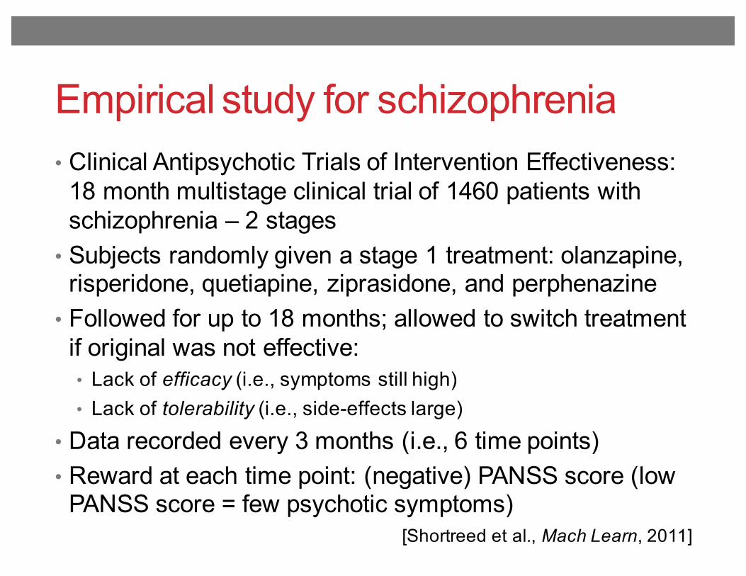
Empirical study for schizophrenia• Clinical Antipsychotic Trials of Intervention Effectiveness:

18 month multistage clinical trial of 1460 patients with schizophrenia – 2 stages

• Subjects randomly given a stage 1 treatment: olanzapine, risperidone, quetiapine, ziprasidone, and perphenazine

• Followed for up to 18 months; allowed to switch treatment if original was not effective:• Lack of efficacy (i.e., symptoms still high)• Lack of tolerability (i.e., side-effects large)

• Data recorded every 3 months (i.e., 6 time points)• Reward at each time point: (negative) PANSS score (low

PANSS score = few psychotic symptoms)[Shortreed et al., Mach Learn, 2011]

Empirical study for schizophrenia

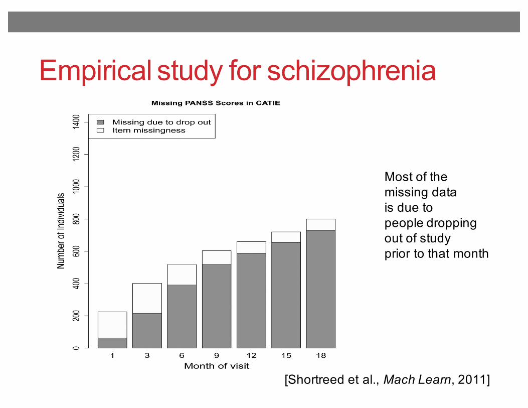
[Shortreed et al., Mach Learn, 2011]Fig. 1.Barplot of missing PANSS scores in the CATIE study. The total height of the bar shows theabsolute number of people who have a missing PANSS score at each of these monthly visits.The dark grey area represents the number of people who have missing PANSS scorebecause they dropped out of the study prior to that month. The unshaded area is the numberof missing PANSS scores due to item missingness. The missing data pattern for other time-varying patient information collected during the CATIE study is similar to the missing datapattern shown here.

Shortreed et al. Page 27

Mach Learn. Author manuscript; available in PMC 2011 July 26.

NIH

-PA

Author M

anuscriptN

IH-P

A A

uthor Manuscript

NIH

-PA

Author M

anuscript

Most of themissing datais due topeople droppingout of studyprior to that month

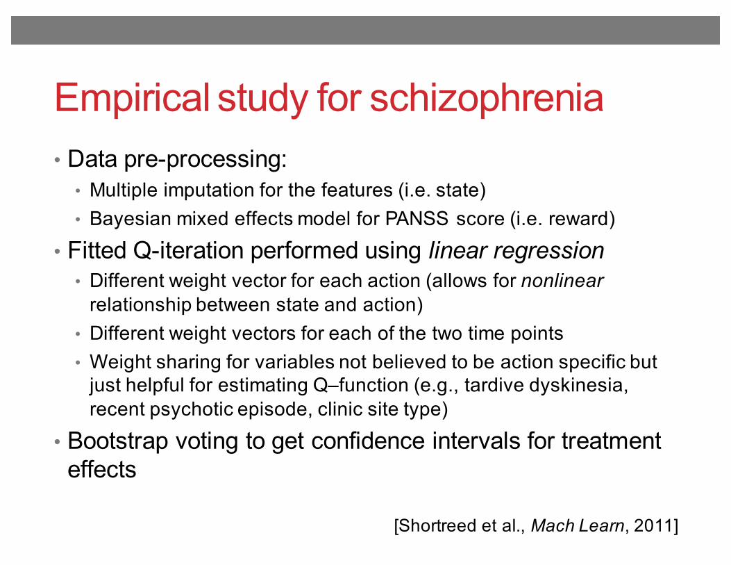
Empirical study for schizophrenia• Data pre-processing:

• Multiple imputation for the features (i.e. state)• Bayesian mixed effects model for PANSS score (i.e. reward)

• Fitted Q-iteration performed using linear regression• Different weight vector for each action (allows for nonlinear

relationship between state and action)• Different weight vectors for each of the two time points• Weight sharing for variables not believed to be action specific but

just helpful for estimating Q–function (e.g., tardive dyskinesia, recent psychotic episode, clinic site type)

• Bootstrap voting to get confidence intervals for treatment effects

[Shortreed et al., Mach Learn, 2011]



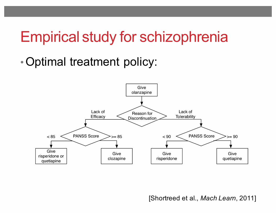
• Optimal treatment policy:

Fig. 3.Optimal treatment policy learned from 25 imputations of the CATIE data, with the totalreward defined as the negative area under the PANSS curve for the 18 months of the CATIEstudy. The state representation is defined in Section 3.1 and the Q-function form used isdescribed in Section 4.2



NIH

-PA Author Manuscript

NIH


NIH




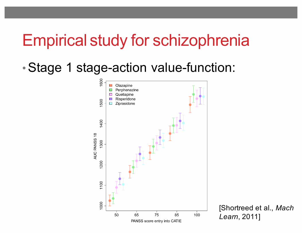
• Stage 1 stage-action value-function:

Fig. 6.Estimates and 95% confidence intervals for stage 1 state-action value-function. The circlerepresents the point estimate for the value of each action given the PANSS score indicatedon the horizontal axis. The different stage 1 treatments are represented by the colorsindicated in the legend.



NIH

-PA

Author M

anuscriptN

IH-P

A A

uthor Manuscript

NIH

-PA

Author M

anuscript



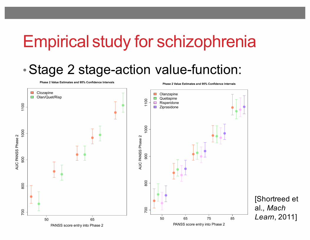
• Stage 2 stage-action value-function:

Fig. 7.Estimates and 95% confidence intervals for stage 2 state-action Q-function. The circlerepresents the point estimates of the state-action value function for each action given thePANSS score indicated on the horizontal axis. The various stage 2 treatments arerepresented by the colors indicated in the legend.



NIH

-PA

Author M

anuscriptN

IH-P

A A

uthor Manuscript

NIH

-PA

Author M

anuscript

Fig. 7.Estimates and 95% confidence intervals for stage 2 state-action Q-function. The circlerepresents the point estimates of the state-action value function for each action given thePANSS score indicated on the horizontal axis. The various stage 2 treatments arerepresented by the colors indicated in the legend.



NIH

-PA

Author M

anuscriptN

IH-P

A A

uthor Manuscript

NIH

-PA

Author M

anuscript

Measuring convergence in fitted Q-iteration

As a baseline, we applied Q-learning to the training data tolearn the mapping of continuous states to Q-values, withfunction approximation using a three-layer feedforwardneural network. The network is trained using Adam, anefficient stochastic gradient-based optimizer (Kingma andBa [2014]), and l2 regularization of weights. Each patientadmission k is treated as a distinct episode, with on the or-der of thousands of state transitions in each; the networkweights are incrementally updated following each transi-tion. Studying the change between successive episodes inthe predicted Q-values for all state-action pairs in the train-ing set (Figure 4), it is unclear whether the algorithm suc-ceeds in converging within the 1,800 training episodes.

Figure 4: Convergence of ˆQ(s, a) using Q-learning.

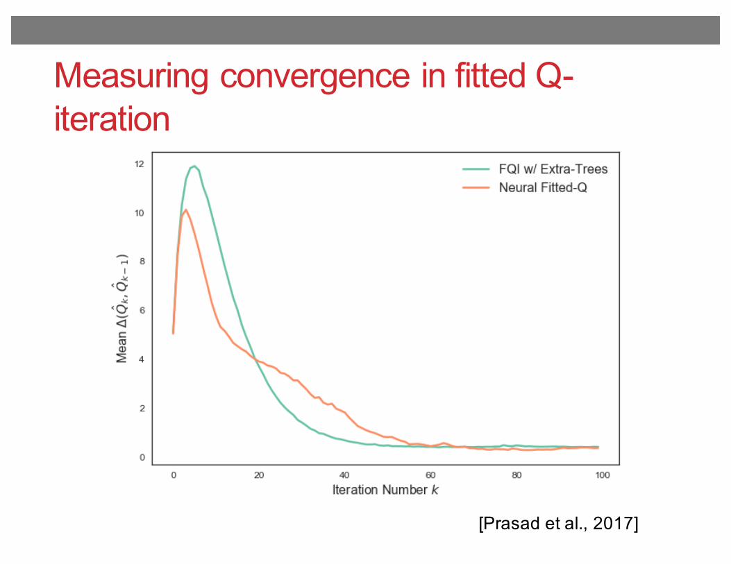
We then explored the use of FQI to learn our Q-function,first running with an Extra-Trees for function approxima-tion. In our implementation, each iteration of FQI is per-formed on a random subset of 10% of all transitions in thetraining set, as described in Algorithm 1, such that on aver-age, each sample is seen in a tenth of all iterations. Thoughsampling increases the total number of iterations requiredfor convergence, it yields significant speed-ups in buildingtrees at each iteration, and hence in total training time. Theensemble regressor learns 50 trees, with regularization inthe form of a minimum leaf node size of 20 samples. Wepresent here results with FQI performed for a fixed numberof 100 iterations, though it is possible to use a convergencecriterion of the form �(Qk, Qk�1) " for early stopping,to speed up training further.

For comparison, we used he same methods to run FQIwith neural networks (NFQ) in place of tree-based regres-sion: we train a feedforward network with architecture andtechniques identical to those applied in our function ap-proximation for Q-learning. Convergence of the estimatedQ-function for both regressors is measured by the meanchange in the estimate ˆQ for transitions in the training set(Figure 5) which shows that the algorithm takes roughly60 iterations to converge in both cases. However, NFQyields approximately a four-fold gain in runtime speed, as

expected, since with neural networks we can simply updateweights rather than retraining fully at each iteration.

Figure 5: Convergence of estimated Q using FQI, given bythe mean change in ˆQ(s, a) over successive iterations.

The estimated Q-functions from FQI with Extra-Trees(FQIT) and from NFQ are then used to evaluate the op-timal action, i.e. that which maximizes the value of thestate-action pair, for each state in the training set. We canthen train policy functions ⇡(s) mapping a given patientstate to the corresponding optimal action a 2 A. To al-low for clinical interpretation of the final policy, we chooseto train an Extra-Trees classifier with an ensemble of 100trees to represent the policy function.

The relative importance assigned to the top 24 features inthe state space for the policy trees learnt, when training onoptimal actions from both FQIT and NFQ, show that thefive vitals ranking highest in importance across the twopolicies are arterial O2 pressure, arterial pH, FiO2, O2

flow and PEEP set (Figure 6). These are as expected—Arterial pH, FiO2, and PEEP all feature in our preliminaryHUP guidelines for extubation criteria, and there is con-siderable literature suggesting blood gases are an impor-tant indicator of readiness for weaning (Hoo [2012]). Onthe other hand, oxygen saturation pulse oxymetry (SpO2)which is also included in HUP’s current extubation crite-ria, is fairly low in ranking. This may be because thesemeasurements are highly correlated with other factors inthe state space, such as arterial O2 pressure (Collins et al.[2015]), that account for its influence on weaning more di-rectly. The limited importance assigned to heart rate andrespiratory rate, which can serve as indicators of bloodpressure and blood gases, are also likely to be explainedby this dependence between vitals.

In terms of demographics, weight and age play a signifi-cant role in the weaning policy learnt: weight is likely toinfluence our sedation policy specifically, as dosages aretypically adjusted for patient weight, while age is stronglycorrelated with a patient’s speed of recovery, and hence thetime necessary on ventilator support.

[Prasad et al., 2017]

Playing Atari with deep reinforcement learning

[Mnih et al., 2015]

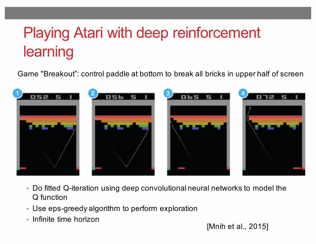
Game "Breakout”: control paddle at bottom to break all bricks in upper half of screen

• Do fitted Q-iteration using deep convolutional neural networks to model the Q function

• Use eps-greedy algorithm to perform exploration• Infinite time horizon

Documents

MACHINE LEARNING FOR HEALTHCARE - GitHub Pages · MACHINE LEARNING FOR HEALTHCARE 6.S897, HST.S53 ... (Thanks to Peter Bodik for slides on reinforcement learning) Lecture 13: Finding