Machine learning methods with applications to

precipitation and streamflow

William W. HsiehDept. of Earth, Ocean & Atmospheric Sciences,

The University of British Columbiahttp://www.ocgy.ubc.ca/~william

Collaborators: Alex Cannon, Carlos Gaitan & Aranildo

Lima

2

Nonlinear regression

Linear regression (LR):

Neural networks (NN/ANN):

Adaptive basis fns hj

Cost function J minimized to solve for the weights

Here J is the mean squared error.

Underfit and overfit:

3

Why is climate more linear than weather?[Yuval & Hsieh, 2002. Quart. J. Roy. Met. Soc.]

4

Curse of the central limit theoremCentral limit theorem says averaging weather data

makes climate data more Gaussian and linear => no advantage using NN!

Nowadays, climate is not just the mean of the weather data, but can be other types of statistics from weather data, E.g. climate of extreme weather

Use NN on daily data, then compile climate statistics of extreme weather

=> Can we escape from the curse of the central limit theorem?

5

Statistical downscalingGlobal climate models (GCM) have poor spatial

resolution

(a) Dynamical downscaling: imbed regional climate model (RCM) in the GCM

(b) Statistical downscaling (SD): Use statistical/machine learning methods to downscale GCM output.

Statistical downscaling at 10 stations in Southern Ontario & Quebec. [Gaitan, Hsieh & Cannon, Clim.Dynam. 2014]

Predictors (1961-2000) from the NCEP/NCAR Reanalysis interpolated to the grid (approx. 3.75° lat. by 3.75° lon.) used by the Canadian CGCM3.1.

6

7

How to validate statistical downscaling in future climate?

Following Vrac et al. (2007), use regional climate model (RCM) output as pseudo-observations.

CRCM 4.2 provides 10 “pseudo-observational” sites For each site, downscale from 9 surrounding CGCM 3.1 grid

cells:

6 predictors/cell : Tmax,Tmin, surface u, v, SLP, precipitation.

6 predictors/cell x 9 cells = 54 predictors 2 Periods:

1971 - 2000 (20th century climate: 20C3M run)

2041 – 2070 (future climate: SRES A2 scenario)

8

10 meteorological stations

Precipitation Occurrence Models

Using the 54 available predictors and a binary predictand (precip./ no precip), we implemented the following models:

Linear Discriminant classifierNaive Bayes classifierkNN (k nearest neighbours) classifier (45 nearest neighbours)

Classification TreeTreeEnsemble: Ensemble of classification trees.ANN-C: Artificial Neural Network Classifier.

9

10Persistence Discriminant naïve-Bayes kNN ClassTree TreeEnsem. ANN-C

Peirce skill score (PSS) for downscaled precipitation occurrence:

20th Century (20C3M) and future (A2) periods.

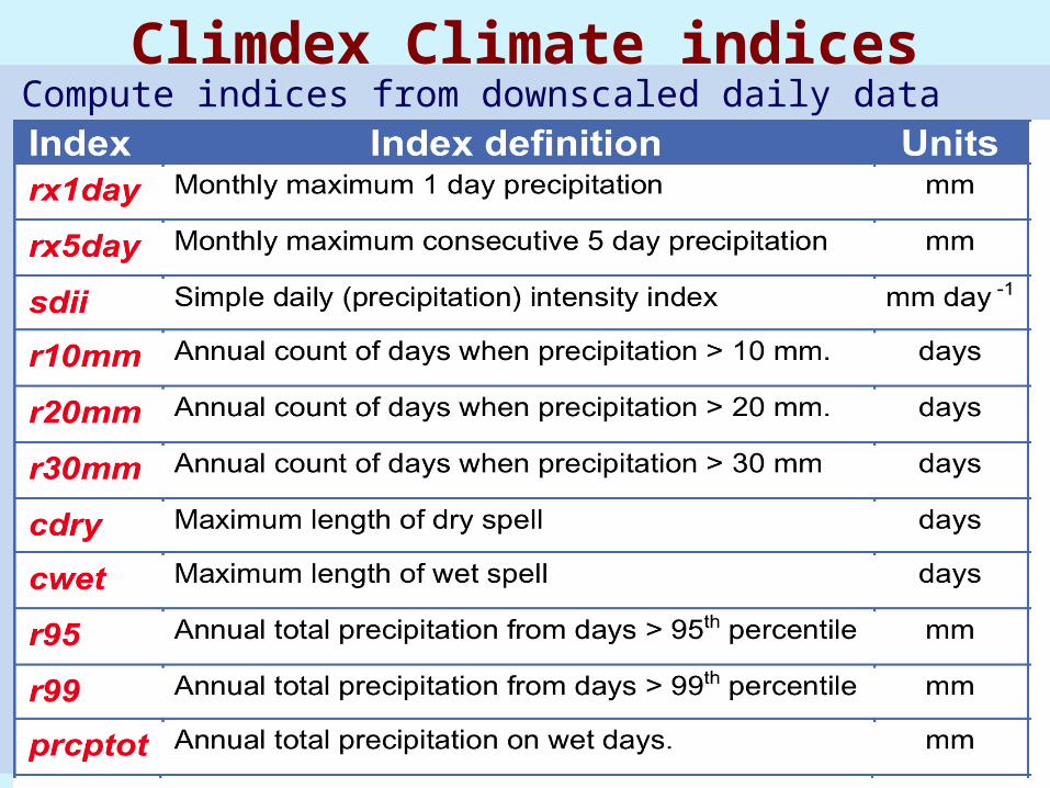
Climdex Climate indices

11

Compute indices from downscaled daily data

12

ANN-F

ARES-F

SWLR-F

IOA

20C3M A2

Index of agreement (IOA) of climate indicesANN-F

ARES-F

SWLR-F

13ANN-F ARES-F SWLR-F

Differences between the IOA of future (A2) and 20th Century (20C3M) climates

14

Conclusion

Use NN on daily data, then compile climate statistics of extreme weather

=> beat linear method => escaped from the curse of the central limit

theorem

15

Extreme learning machine (ELM): [G.-B. Huang]

ANN:

ELM: Choose the weights (wij and w0j) of the hidden neurons randomly.

Only need to solve for aj and a0 by linear least squares.

ELM turns nonlinear regression by NN into a linear regression problem!

16

Tested ELM on 9 environmental datasets [Lima, Cannon and Hsieh, Environmental Modelling & Software, under revision]

Goal is to develop ELM into nonlinear updateable model output statistics (UMOS).

17

Deep learning

18

Spare slides

Compare 5 models over 9 environmental datasets[Lima, Cannon & Hsieh. Environmental Modelling & Software

(under revision)]

MLR = multiple linear regressionANN = Artificial neural network SVR-ES = Support vector regression (with

Evolutionary Strategy)RF = random forestELM-S = Extreme Learning Machine (with scaled

weights)Optimal number of hidden neurons in ELM chosen over validation data by a simple hill climbing algorithm.

Compare models in terms of:

RMSE skill score = 1 – RMSE/RMSEMLR

t = cpu time19

20

RMSE skill score (relative to MLR)

21

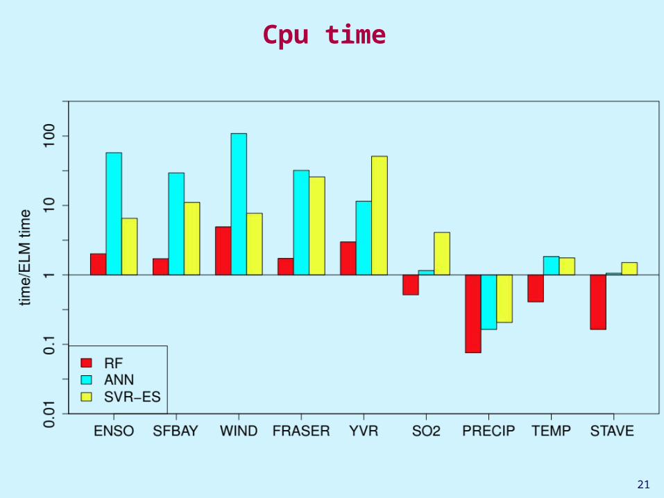
Cpu time

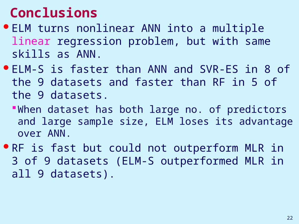
ConclusionsELM turns nonlinear ANN into a multiple linear

regression problem, but with same skills as ANN.ELM-S is faster than ANN and SVR-ES in 8 of the 9

datasets and faster than RF in 5 of the 9 datasets.When dataset has both large no. of predictors and large sample size, ELM loses its advantage over ANN.

RF is fast but could not outperform MLR in 3 of 9 datasets (ELM-S outperformed MLR in all 9 datasets).

22

Online sequential learningPreviously, we used ELM for batch learning. When new

data arrive, need to retrain model using the entire data record => very expensive.

Now use ELM for “online sequential learning” (i.e. as new data arrive, update the model with only the new data)

For multiple linear regression (MLR), online sequential MLR (OS-MLR) is straightforward. [Envir.Cda’s updateable MOS (model output statistics), used to post-process NWP model output, is based on OS-MLR]

Online sequential ELM (OS-ELM) (Liang et al. 2006, IEEE Trans. Neural Networks) is easily derived from OS-MLR.

23

Predict streamflow at Stave, BC at 1-day lead.23 potential predictors (local observations, GFS

reforecast data, climate indices) [same as Rasouli et al. 2012].

Data during 1995-1997 used to find the optimal number of hidden neurons (3 for ANN and 27 for ELM), and to train the first model.

New data arrive (a) weekly, (b) monthly or (c) seasonally. Validate forecasts for 1998-2001.

5 models: MLR, OS-MLR, ANN, ELM, OS-ELMCompare correlation (CC), mean absolute error

(MAE), root mean squared error (RMSE) and cpu time

24

25

26

ConclusionWith new data arriving frequently, OS-ELM

provides a much cheaper way to update & maintain a nonlinear regression model.

Future researchOS-ELM retains the information from all the data

it has seen. If data are non-stationary, need to forget the older data.

Adaptive OS-ELM has an adaptive forgetting factor.

27